short-term and long-term educational mobility of families
TRANSCRIPT

California Center for Population Research On-Line Working Paper Series
Short-Term and Long-Term Educational Mobility of Families: A Two Sex Approach
Xi Song and Robert D. Mare
PWP-CCPR-2014-013
September 2014

Song‐Mare: Two‐Sex Approach
SHORT-TERM AND LONG-TERM EDUCATIONAL MOBILITY OF FAMILIES:
A TWO-SEX APPROACH*
XI SONG AND ROBERT D. MARE
University of California, Los Angeles
Version: September 2014
Keywords: Educational mobility; multigenerational; two-sex model; assortative mating
Word count (including text, abstract, footnotes): 8,248, 7 tables, 3 figures
* Send correspondence to Xi Song, Department of Sociology, University of California, Los Angeles, 264 Haines Hall, Los Angeles, CA 90095-1551, USA; email: [email protected]. We are grateful to Cameron Campbell, Hal Caswell, Thomas DiPrete, Mark Handcock, Benjamin Jarvis, Sung Park, Judith Seltzer, Florencia Torche, and Shripad Tuljapurkar for their suggestions. Earlier versions of this paper were presented at the biodemography workshop at Stanford, May 6-8, 2013; the spring meeting of ISA Research Committee on Social Stratification (RC28), Trento, May 16-18, 2013; and the annual meeting of the American Sociological Association, August 10-13, 2013, New York. Please do not cite or circulate without the authors’ permission. While conducting this analysis, the authors received support from the National Science Foundation (SES-1260456). The authors also benefited from facilities and resources provided by the California Center for Population Research at UCLA (CCPR), which receives core support (R24-HD041022) from the Eunice Kennedy Shriver National Institute of Child Health and Human Development (NICHD).
Song‐Mare: Two‐Sex Approach
SHORT-TERM AND LONG-TERM EDUCATIONAL MOBILITY OF FAMILIES:
A TWO-SEX APPROACH
ABSTRACT
We investigate how families reproduce and pass on their educational advantages to succeeding
generations from a multigenerational perspective. Unlike traditional mobility studies that
typically focus on one-sex influences from fathers to sons, we rely on a two-sex approach that
accounts for the marriage market interaction between males and females, which includes
educational assortative mating in both parent and grandparent generations and intergenerational
transmission of educational status through both the male and female sides of families over three
generations. Using data from the Panel Study of Income Dynamics, we approach this issue from
both a short-term and a long-term perspective. For the short term, grandparents’ educational
attainments have a direct association with grandchildren’s education as well as an indirect
association that is mediated by parents’ education and demographic behaviors. For the long term,
initial educational advantages of families may benefit as many as three subsequent generations,
but such advantages are later offset by the lower fertility of highly educated persons. Yet all
families eventually achieve the same educational distribution of descendants because of
intermarriages between high- and low-education origin families.
Song‐Mare: Two‐Sex Approach
1
SHORT-TERM AND LONG-TERM EDUCATIONAL MOBILITY OF FAMILIES:
A TWO-SEX APPROACH
INTRODUCTION
Educational attainment is a source of upward social mobility for individuals and families.
Higher education changes not only the social circumstances of the present generation but also
potentially the educational prospects of children, grandchildren and subsequent generations of a
family. This study investigates the educational reproduction of families—that is, how
successfully families reproduce their educational advantages in subsequent generations. An
examination of this question involves a joint study of demographic reproduction and
intergenerational social mobility. Our broad definition of families refers to not only nuclear and
extended families, but also lineages that include distant descendants who share the same ancestry.
Unlike traditional mobility studies that focus on parent to offspring mobility, we examine
both “short-term” and “long-term” social mobility from a multigenerational perspective. For
short-term mobility, which refers to educational mobility across three generations, we assess the
validity of the Markovian assumption that underpins most mobility research (Mare 2011). Two-
generation mobility studies implicitly assume that grandparents’ influence on grandchildren
occurs only through their influence on parents, who in turn influence their children. This
assumption underestimates the degree of multigenerational influence, however, if (1)
grandparents’ statuses directly affect grandchildren’s statuses, net of their intervening effect via
parents’ statuses, or (2) grandparents influence the grandchild generation through parents’ and
grandchildren’s demographic outcomes, such as their marriage, fertility, and mortality. We

Song‐Mare: Two‐Sex Approach
2
examine these two mechanisms for American families using data from the Panel Study of
Income Dynamics.
For long-term mobility, we assess differences in the educational composition of progeny
from high- and low-education families in an indefinite future. We investigate how individuals
who differ in educational attainment may yield different education distributions among their
progeny several generations hence. Our analyses shed light on whether an increase in education
of families at one generation can permanently change the educational prospects for future
descendants. Our approach is to use information on assortative mating, fertility, and
intergenerational social mobility based on our short-term analyses to simulate the educational
distribution of families in subsequent generations, and to see whether the education distributions
of descendants from high- and low-education families converge or remain distinct. In a simple
Markov model for educational mobility, the educational distribution of families converges to the
same distribution regardless of where a family begins. Yet such a prediction only applies to the
mobility process, whereas the interplay between social mobility and reproductive success may
further complicate the dynamics of the trend (Lam 1986; Maralani 2013; Mare 1997; Mare and
Maralani 2006; Mare and Song 2014; Matras 1961, 1967; Preston 1974).
Building upon the two-sex demographic model of IQ inheritance in Preston and
Campbell (1993) and the “birth matrix-mating rule (BMMR) model” in Pollak (1986, 1987,
1990), we develop a two-sex multigenerational demographic model of social mobility. .
Compared with the one-sex model, our two-sex approach incorporates two new features: First, it
takes account of educational assortative mating from the standpoint of both the male and female
populations, in both the parent and the grandparent generations, in creating unequal educational
resources across families. Second, it examines roles of both parents and all four grandparents,
Song‐Mare: Two‐Sex Approach
3
rather than one sex alone in offspring’s educational mobility. Therefore, it provides a more
complete account of the formation of multigenerational inequality between families through the
interaction of males and females.
Our short-term analyses suggest that grandparents’ educational attainments directly
influence grandchildren’s educational outcomes independent of parents’ education. On average,
all four grandparents have similar effects on their grandchildren’s educational attainment.
Grandparents also influence grandchildren’s education by influencing parents’ marriage and
fertility behaviors. Our long-term analyses show different predictions using one-sex and two-sex
approaches. The former suggests persistent differences in the educational composition of
progeny between families, whereas the latter suggests that the differences eventually disappear.
The two-sex model takes account of intermarriages between families with different education
levels, which eliminate the ability of highly educated individuals to secure a long run educational
advantage for their progeny.
This study also advances our understanding of multigenerational inequality of families
(e.g., Chan and Boliver 2013; Mare 2011, 2014; Pfeffer 2014; Zeng and Xie 2014). We show
that multigenerational influences are shaped by the combination of families’ mobility and
demographic behaviors and transmitted through both sexes. Such mechanisms have implications
for unequal educational outcomes between families in the short term and the long term. The
paper concludes with a taxonomy of approaches to the analysis of mobility, which includes one-
and two-sex models, two generation and multi-generation models, and models with and without
demographic processes.

Song‐Mare: Two‐Sex Approach
4
SHORT-TERM AND LONG-TERM MULTIGENERATIONAL SOCIAL MOBILITY
Social mobility studies typically rely on a short-term framework, mostly focusing on
intergenerational mobility from parents to offspring, (e.g., Blau and Duncan 1967; Erikson and
Goldthorpe 1992; Featherman and Hauser 1978; Hout 1983; 1988) and occasionally including
grandparents as well (Hodge 1966; Warren and Hauser 1997). The lack of three-generation
mobility studies is justified by the Markovian assumption that associations between adjacent
generations suffice to explain mobility processes over multiple generations (Mare 2011). Empirical
research testing the validity of the Markovian assumption is sparse and inconclusive. For
example, using data from the Wisconsin Longitudinal Studies, two studies found that
grandparents play a trivial role in directly influencing their grandchildren’s educational outcomes
(Warren and Hauser 1997; Jæger 2012). Similar findings also appear in a study of Finland (Erola
and Moisio 2007). By contrast, several recent studies have challenged the Markovian assumption,
showing that grandparents with favorable social characteristics can transmit their advantages to
their grandchildren, net of parents’ characteristics (e.g., Chan and Boliver 2013; Hertel and
Groh-Samberg 2014; Wightman and Danziger 2014; Zeng and Xie 2014).
Regardless of whether the intergenerational transmission of socioeconomic status is
Markovian, however, grandparents may also influence grandchildren’s socioeconomic status
through influencing parents’ demographic behaviors (Mare 2011; Mare and Song 2014). Just as
the impact of one generation on the next in a two generation model comes about through the
joint effects of intergenerational transmission and differential demographic behavior (Mare and
Maralani 2006; Maralani 2013), grandparents’ socioeconomic characteristics can influence
parents’ marriage prospects, mate choices, and fertility decisions, all of which make up the
“family background” of the grandchildren and subsequently influence their life chances. Even if
Song‐Mare: Two‐Sex Approach
5
parents’ demographic behaviors are independent of grandparents’ social characteristics, parents’
decisions on whether, when, and whom to marry and how many children to have children change
grandparents’ influences on grandchildren. Grandparents with many children and grandchildren
will have a much greater capacity to affect subsequent generations, whereas persons cannot pass
on their advantages or disadvantages beyond the next generation if their children are childless.
The effects of individuals’ characteristics on the characteristics of their progeny include
both their direct impacts on their children and grandchildren and also their potential long run
impacts across a larger number of generations. Although most demographic effects die out after
several generations, it remains possible that some combinations of multigenerational social
mobility and demographic patterns may lead to longer run effects. If all families have the same
fertility, mortality, and marriage behaviors but unequal mobility opportunities determined by the
parent generation’s educational attainment, the Markov assumption implies that families
eventually lose their influences because descendants from all families converge to the same
educational distribution. The mobility process itself removes all initial educational advantages or
disadvantages of families (e.g., Bartholomew 1982). Under these conditions, multigenerational
influences in the educational reproduction of families are transient, suggesting that short-term
inequality between families within three generations does not result in long-term
multigenerational inequality.
The interplay between mobility and demography, however, further complicates the trend
of long-term educational reproduction of families. In the presence of positive association
between fertility and socioeconomic status, the multigenerational influences of social mobility
patterns and differential fertility are mutually reinforcing: men in high-status families are more
likely to have high-status sons and to have more sons who survive to adulthood (Mare and Song

Song‐Mare: Two‐Sex Approach
6
2014). As a result their descendants account for a disproportionately large share of the high-
status population in later generations. In contemporary societies where the association between
fertility and socioeconomic status is negative, on the other hand, offspring from high-education
families are more likely to attain high education, but the overall advantages of high-education
families may be offset by their lower fertility. Therefore, the educational reproduction of high-
education families in terms of their total number of high-education descendants in later
generations depends on the relative strength of mobility advantages and differential net fertility.
This paper extends the two-generation joint demographic and social mobility approach
used in previous studies (e.g., Mare and Maralani 2006; Maralani 2013; Preston 1974) to a
multigenerational scenario. Our approach on the multigenerational transmission of educational
inequality in the short-term and long-term incorporates a wider array of social and demographic
processes, which include educational assortative mating, differential marriage and fertility rates
between high-education and low-education couples, and intergenerational transmission of
educational status through both sides of families. To integrate these processes into a
multigenerational model, we need to modify one-sex intergenerational mobility models to look at
both sexes together.
ONE-SEX VERSUS TWO-SEX MOBILITY APPROACHES
A one-sex approach to the study of social mobility is adequate when the socioeconomic
position of families and individuals is reproduced through the line of the same-sex parent,
whether on the maternal or paternal side of the family, and when the availability of suitable
marriage partners is not substantially constrained. In contemporary societies, however, both
parents play a role in determining the economic statuses of families and may have independent
effects on the life chances of their offspring (e.g., Beller 2009). In addition to the two-generation

Song‐Mare: Two‐Sex Approach
7
effects of mothers and fathers, grandmothers and grandfathers on both sides of the family may
affect the life chances of their grandchildren (e.g., Cherlin and Furstenberg 1986). A two-sex
approach can also incorporate demographic mechanisms into the mobility process that are left
out of one-sex models. Several studies have shown the role of interplay between demographic
behaviors and social mobility in the evolution of social inequality (Lam 1986; Matras 1961, 1967;
Mare 1997; Mare and Maralani 2006; Maralani 2013; Preston 1974; Preston and Campbell 1993).
Except for Preston and Campbell’s (1993) study, however, these studies rely on a one-sex
approach, which does not take account of how numbers of men and women, with varying
socioeconomic characteristics, constrain marriage opportunities in a single generation and the
distribution of family backgrounds in subsequent generations (Pollak 1990; Schoen 1981; Mare
and Schwartz 2006). Overall, the two-sex approach in this paper consists of two components: a
mobility component that examines influences of grandparents on grandchildren through both
paternal and maternal family lines, and a demographic component that examines educational
assortative mating of fathers and mothers in the marriage market in order to form families for the
next generation. A comparison of the two-sex results with those from a one-sex approach
illustrates the extent to which conclusions about the multigenerational mobility process is an
artifact of the approach used in the analysis.
SOCIAL AND DEMOGRAPHIC MOBILITY MODELS
One-Sex Approach
We begin with the one-sex model for the influences of parents’ education on the
educational outcome of offspring. Following Mare and Maralani (2006), we specify the one-sex
model as

Song‐Mare: Two‐Sex Approach
8
| ∙ ∙ ∙ | (1)
where | denotes the number of men (woman) in the offspring’s generation who are in
education group j and have fathers (mothers) in education group i. denotes the number of men
(women) in the paternal (maternal) generation who are in education group i. denotes the
probability that a man (woman) in education group i gets married. denotes the expected
number of sons (daughters) who are born to a man (woman) in education group i and survive to
adulthood. | denotes the probability that a son (daughter) born to a man (woman) in education
group i enters education group j.
A three-generation version of the model further incorporate grandparents’ education;
therefore, the marriage component m, the fertility component f and the mobility component p
depend on both fathers’ (mothers’) and grandfathers’ (grandmothers’) educational attainments.
| ∙ ∙ ∙ | (2)
where | denotes the number of men (woman) in the offspring’s generation (G3) who are in
education group j and have grandfathers (grandmothers) in education group i and fathers
(mothers) in education group k. denotes the number of men (women) in the paternal
(maternal) generation (G2) who are in education group k and have fathers (G1) in education
group i. denotes the probability that a man (woman) in education group k with a father
(mother) in education group i gets married. denotes the expected number of sons (daughters)
who are born to a father (mother) in education group k and a grandfather (grandmother) in
education group i and survive to adulthood. | denotes the probability that a son (daughter)
born to a father (mother) in education group k and a grandfather (grandmother) in education
group i will enter education group j. This model accounts for differentials in marriage behavior
by men’s (or women’s) level of education, but only under very restrictive assumptions such as
Song‐Mare: Two‐Sex Approach
9
that the availability of partners of the opposite sex is completely unconstrained or that the
matching of men’s and women’s educational attainments follows complete male dominance or
complete female dominance. The one-sex model does not adequately take account of the
interdependence of the male and female populations.
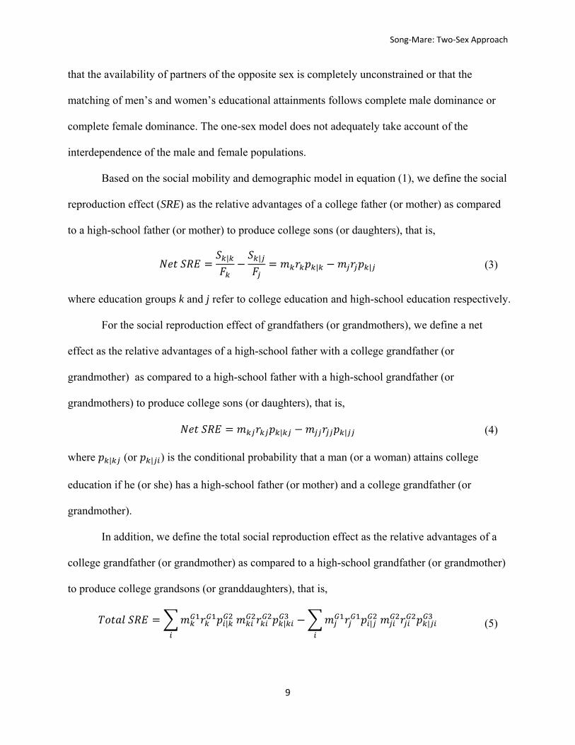
Based on the social mobility and demographic model in equation (1), we define the social
reproduction effect (SRE) as the relative advantages of a college father (or mother) as compared
to a high-school father (or mother) to produce college sons (or daughters), that is,
| |
| | (3)
where education groups k and j refer to college education and high-school education respectively.
For the social reproduction effect of grandfathers (or grandmothers), we define a net
effect as the relative advantages of a high-school father with a college grandfather (or
grandmother) as compared to a high-school father with a high-school grandfather (or
grandmothers) to produce college sons (or daughters), that is,
| | (4)
where | (or | ) is the conditional probability that a man (or a woman) attains college
education if he (or she) has a high-school father (or mother) and a college grandfather (or
grandmother).
In addition, we define the total social reproduction effect as the relative advantages of a
college grandfather (or grandmother) as compared to a high-school grandfather (or grandmother)
to produce college grandsons (or granddaughters), that is,
| | | | (5)
Song‐Mare: Two‐Sex Approach
10
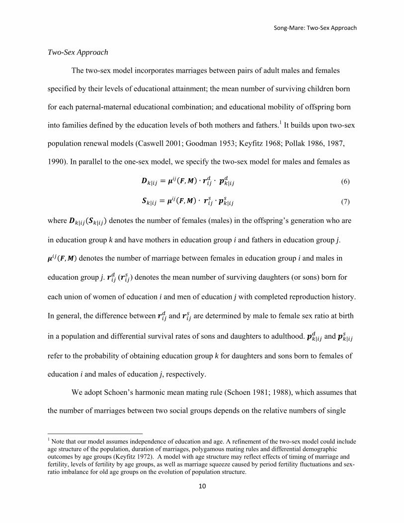
Two-Sex Approach
The two-sex model incorporates marriages between pairs of adult males and females
specified by their levels of educational attainment; the mean number of surviving children born
for each paternal-maternal educational combination; and educational mobility of offspring born
into families defined by the education levels of both mothers and fathers.1 It builds upon two-sex
population renewal models (Caswell 2001; Goodman 1953; Keyfitz 1968; Pollak 1986, 1987,
1990). In parallel to the one-sex model, we specify the two-sex model for males and females as
| , ∙ ∙ | (6)
| , ∙ ∙ | (7)
where | | denotes the number of females (males) in the offspring’s generation who are
in education group k and have mothers in education group i and fathers in education group j.
, denotes the number of marriage between females in education group i and males in
education group j. ( ) denotes the mean number of surviving daughters (or sons) born for
each union of women of education i and men of education j with completed reproduction history.
In general, the difference between and are determined by male to female sex ratio at birth
in a population and differential survival rates of sons and daughters to adulthood. | and |
refer to the probability of obtaining education group k for daughters and sons born to females of
education i and males of education j, respectively.
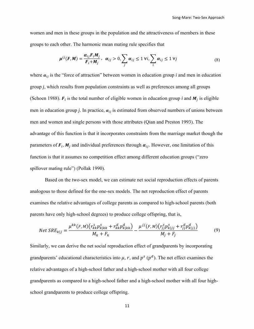
We adopt Schoen’s harmonic mean mating rule (Schoen 1981; 1988), which assumes that
the number of marriages between two social groups depends on the relative numbers of single
1 Note that our model assumes independence of education and age. A refinement of the two-sex model could include age structure of the population, duration of marriages, polygamous mating rules and differential demographic outcomes by age groups (Keyfitz 1972). A model with age structure may reflect effects of timing of marriage and fertility, levels of fertility by age groups, as well as marriage squeeze caused by period fertility fluctuations and sex-ratio imbalance for old age groups on the evolution of population structure.
Song‐Mare: Two‐Sex Approach
11
women and men in these groups in the population and the attractiveness of members in these
groups to each other. The harmonic mean mating rule specifies that
, , 0, 1 ∀ , 1 ∀ (8)
where is the “force of attraction” between women in education group i and men in education
group j, which results from population constraints as well as preferences among all groups
(Schoen 1988). is the total number of eligible women in education group i and is eligible
men in education group j. In practice, is estimated from observed numbers of unions between
men and women and single persons with those attributes (Qian and Preston 1993). The
advantage of this function is that it incorporates constraints from the marriage market though the
parameters of , and individual preferences through . However, one limitation of this
function is that it assumes no competition effect among different education groups (“zero
spillover mating rule”) (Pollak 1990).
Based on the two-sex model, we can estimate net social reproduction effects of parents
analogous to those defined for the one-sex models. The net reproduction effect of parents
examines the relative advantages of college parents as compared to high-school parents (both
parents have only high-school degrees) to produce college offspring, that is,
|, | | , | |
(9)
Similarly, we can derive the net social reproduction effect of grandparents by incorporating
grandparents’ educational characteristics into , , and ( ). The net effect examines the
relative advantages of a high-school father and a high-school mother with all four college
grandparents as compared to a high-school father and a high-school mother with all four high-
school grandparents to produce college offspring.
Song‐Mare: Two‐Sex Approach
12
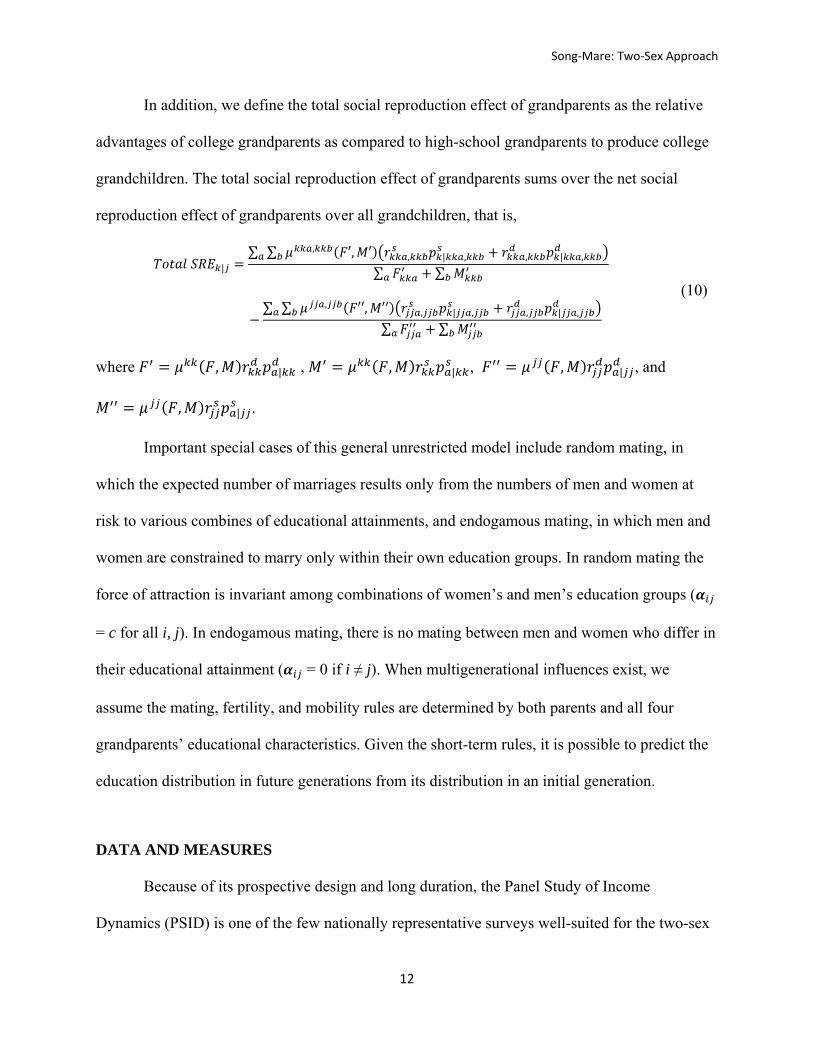
In addition, we define the total social reproduction effect of grandparents as the relative
advantages of college grandparents as compared to high-school grandparents to produce college
grandchildren. The total social reproduction effect of grandparents sums over the net social
reproduction effect of grandparents over all grandchildren, that is,
|
∑ ∑ , ′, ′ , | , , | ,
∑ ∑
∑ ∑ , ′′, ′′ , | , , | ,
∑ ∑
(10)
where , | , , | , , | , and
, | .
Important special cases of this general unrestricted model include random mating, in
which the expected number of marriages results only from the numbers of men and women at
risk to various combines of educational attainments, and endogamous mating, in which men and
women are constrained to marry only within their own education groups. In random mating the
force of attraction is invariant among combinations of women’s and men’s education groups (
= c for all i, j). In endogamous mating, there is no mating between men and women who differ in
their educational attainment ( = 0 if i ≠ j). When multigenerational influences exist, we
assume the mating, fertility, and mobility rules are determined by both parents and all four
grandparents’ educational characteristics. Given the short-term rules, it is possible to predict the
education distribution in future generations from its distribution in an initial generation.
DATA AND MEASURES
Because of its prospective design and long duration, the Panel Study of Income
Dynamics (PSID) is one of the few nationally representative surveys well-suited for the two-sex

Song‐Mare: Two‐Sex Approach
13
multigenerational analysis formulated above. Begun in 1968, the PSID was conducted annually
until 1997 and biennially thereafter. The study follows targeted respondents according to a
genealogical design. All household members recruited into the PSID in 1968 are considered to
carry the PSID “gene” and are targeted for collection of detailed socioeconomic information.
Members of new households created by the offspring of original targeted household members
retain the PSID “gene” themselves and become permanent PSID respondents.
To create our multigenerational sample, we first obtain a FIMS (Family Identification
Mapping System)2 sample that links PSID respondents (G3) with their parents (G2), who are
also PSID respondents. Based on the retrospective information from the family interview for
household heads and head’s wives (G2), we obtain parental information for the grandparent
generation (G1), who may not be PSID respondents. Therefore, we have information from all of
the four biological grandparents of PSID respondents in G3.3
We create two analytical samples: a mobility sample and a marriage/fertility sample. The
mobility sample includes education information of PSID sample members and their biological
fathers, mothers, and all four grandparents. Individuals who grew up in single-parent families
and thus have incomplete education information for one or several parents and grandparents are
excluded from the analyses. We recode the educational variable into four categories according to
the years of schooling (0-11, 12, 13-15, 16+).
The marriage/fertility sample is generated from the PSID 1985-2011 Marriage History
File, which contains details about retrospective marriage history of eligible people living in a
PSID family at the time of the interview in any wave between 1985 and 2011 (PSID User
2 “Family Identification Mapping System” is a tool developed by the PSID to create intergenerational linked samples (http://simba.isr.umich.edu/FIMS/) 3 This linking method yields a bigger sample size than from a prospective method that links PSID respondents from the first generation to the second and third generations because only a subset of the parents and grandparents of the third generation are themselves PSID respondents.
Song‐Mare: Two‐Sex Approach
14
Manual 2013). We merge the Marriage History File with the 1968-2011 Individual File to find
the education information of individuals and their spouses. Some spouses, however, do not have
follow-up records on the Individual File if they leave the PSID households, because they do not
carry the PSID “gene.” We then rely on household head and wife information from the 1975-
2011 Family File to find out the missing information of spouses. To give each individual in the
marriage/fertility sample the same weight, we restrict our analyses to the first marriage of all
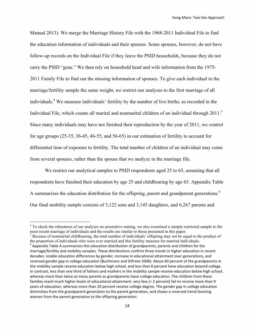
individuals.4 We measure individuals’ fertility by the number of live births, as recorded in the
Individual File, which counts all marital and nonmarital children of an individual through 2011.5
Since many individuals may have not finished their reproduction by the year of 2011, we control
for age groups (25-35, 36-45, 46-55, and 56-65) in our estimation of fertility to account for
differential time of exposure to fertility. The total number of children of an individual may come
from several spouses, rather than the spouse that we analyze in the marriage file.
We restrict our analytical samples to PSID respondents aged 25 to 65, assuming that all
respondents have finished their education by age 25 and childbearing by age 65. Appendix Table
A summarizes the education distribution for the offspring, parent and grandparent generations.6
Our final mobility sample consists of 3,122 sons and 3,145 daughters, and 6,267 parents and
4 To check the robustness of our analyses on assortative mating, we also examined a sample restricted sample to the most recent marriage of individuals and the results are similar to those presented in this paper. 5 Because of nonmarital childbearing, the total number of individuals’ offspring may not be equal to the product of the proportion of individuals who were ever married and this fertility measure for married individuals. 6 Appendix Table A summarizes the education distribution of grandparents, parents and children for the marriage/fertility and mobility samples. These distributions confirm three trends in higher education in recent decades: sizable education differences by gender, increase in educational attainment over generations, and reversed gender gap in college education (Buchmann and DiPrete 2006). About 60 percent of the grandparents in the mobility sample receive education below high school, and less than 8 percent have education beyond college. In contrast, less than one third of fathers and mothers in the mobility sample receive education below high school, whereas more than twice as many parents as grandparents have college education. The children from these families reach much higher levels of educational attainment: very few (< 2 percent) fail to receive more than 9 years of education, whereas more than 20 percent receive college degree. The gender gap in college education diminishes from the grandparent generation to the parent generation, and shows a reversed trend favoring women from the parent generation to the offspring generation.

Song‐Mare: Two‐Sex Approach
15
grandparents with non-missing values. Our marriage sample, which includes respondents who
have non-missing educational information on both parents, consists of 9,683 and 9,867 eligible
males and females respectively. Among these eligible males and females, 7,586 men and 8,100
women are married or were ever married before the last wave in 2011. We restrict the fertility
sample to respondents who have complete educational information of spouse, both parents, and
spouse’s parents, which yields a sample of 13,090 married couples.7
SHORT-TERM MULTIGENERATIONAL INFLUENCES
We begin with analyses based on the one-sex approach, which considers mating, fertility,
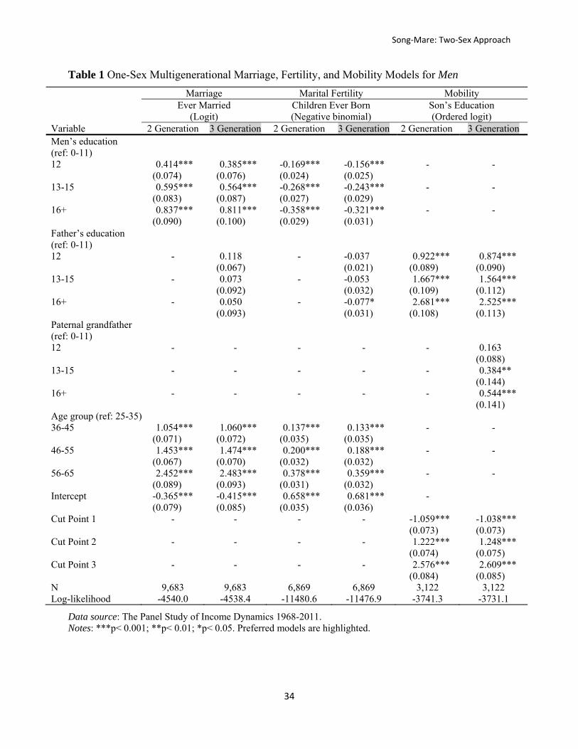
and mobility patterns for sons, fathers, and grandfathers (Table 1), and daughters, mothers, and
grandmothers (Table 2), respectively. For all models, we assume discrete, additive
multigenerational effects, meaning that we do not include associations between an individual’s
educational attainment and interactions between the attainments of their parents and
grandparents. For the sake of simplicity, the models presented in the tables only include
education variables for grandparents, parents, and offspring generations, but we also
experimented with models that include control variables such as race, the number of siblings, and
the age group of the offspring generation, as well as interactions of these variables. The control
variables do not change the results presented below, and we find little evidence for the effects of
these interactions.
The marriage and fertility results in Table 1 and Table 2 suggest that a person’s
likelihood of getting married and the number of children depends on both his or her own and the
7 We do not control for race in our analyses because we are unable to examine racial and educational assortative mating jointly given our sample size. We show the racial distribution of our samples in Appendix Table A, which suggests an overrepresentation of African Americans and an underrepresentation of other races due to the sampling design of PSID.
Song‐Mare: Two‐Sex Approach
16
same-sex parent’s educational attainment. On average, individuals with higher education or
highly educated parents are more likely to get married than their low-education counterparts, but
they tend to have a lower level of fertility. The mobility results are consistent with Hertel and
Groh-Samberg’s (2014) findings that grandfathers’ social class is directly associated with their
grandsons’ socioeconomic attainment.8 Overall, our marriage, fertility, and mobility models are
inconsistent with a simple Markovian assumption, suggesting that grandfathers’ and
grandmothers’ education influences their grandchildren’s education not only indirectly through
fathers’ and mothers’ marriage prospects and fertility, but also through a net direct effect.
[Table 1]
[Table 2]
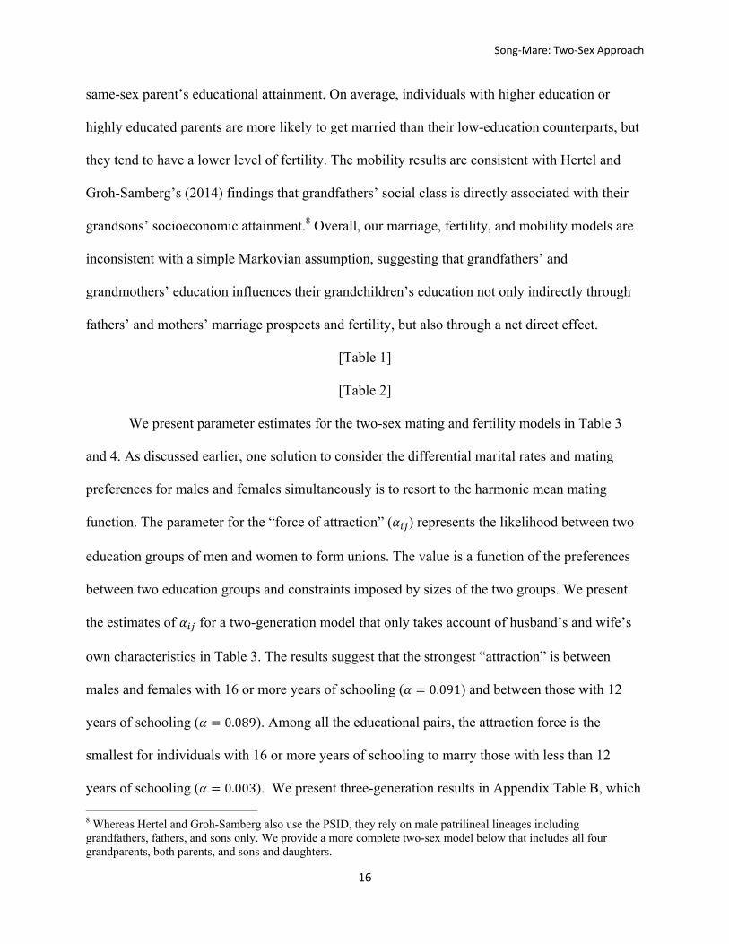
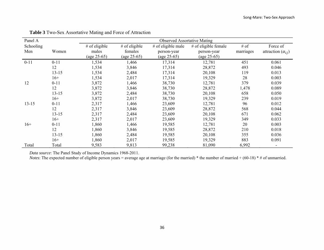
We present parameter estimates for the two-sex mating and fertility models in Table 3
and 4. As discussed earlier, one solution to consider the differential marital rates and mating
preferences for males and females simultaneously is to resort to the harmonic mean mating
function. The parameter for the “force of attraction” ( ) represents the likelihood between two
education groups of men and women to form unions. The value is a function of the preferences
between two education groups and constraints imposed by sizes of the two groups. We present
the estimates of for a two-generation model that only takes account of husband’s and wife’s
own characteristics in Table 3. The results suggest that the strongest “attraction” is between
males and females with 16 or more years of schooling ( 0.091) and between those with 12
years of schooling ( 0.089). Among all the educational pairs, the attraction force is the
smallest for individuals with 16 or more years of schooling to marry those with less than 12
years of schooling ( 0.003). We present three-generation results in Appendix Table B, which
8 Whereas Hertel and Groh-Samberg also use the PSID, they rely on male patrilineal lineages including grandfathers, fathers, and sons only. We provide a more complete two-sex model below that includes all four grandparents, both parents, and sons and daughters.
Song‐Mare: Two‐Sex Approach
17
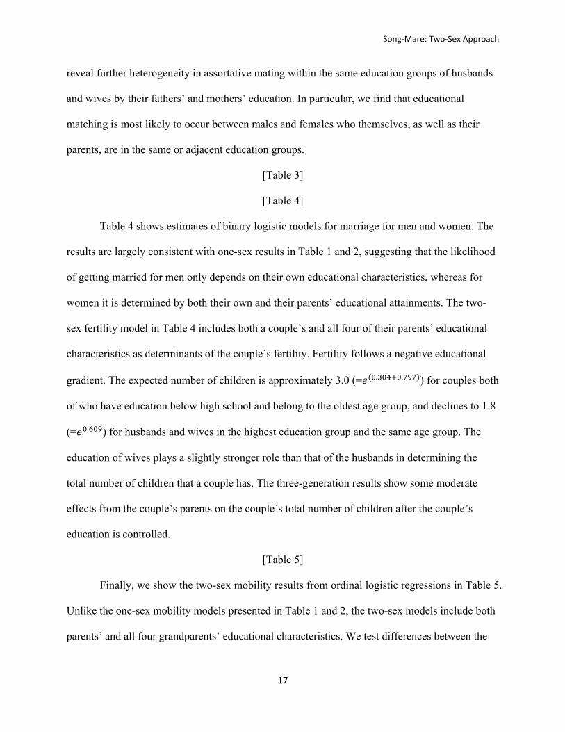
reveal further heterogeneity in assortative mating within the same education groups of husbands
and wives by their fathers’ and mothers’ education. In particular, we find that educational
matching is most likely to occur between males and females who themselves, as well as their
parents, are in the same or adjacent education groups.
[Table 3]
[Table 4]
Table 4 shows estimates of binary logistic models for marriage for men and women. The
results are largely consistent with one-sex results in Table 1 and 2, suggesting that the likelihood
of getting married for men only depends on their own educational characteristics, whereas for
women it is determined by both their own and their parents’ educational attainments. The two-
sex fertility model in Table 4 includes both a couple’s and all four of their parents’ educational
characteristics as determinants of the couple’s fertility. Fertility follows a negative educational
gradient. The expected number of children is approximately 3.0 (= . . ) for couples both
of who have education below high school and belong to the oldest age group, and declines to 1.8
(= . ) for husbands and wives in the highest education group and the same age group. The
education of wives plays a slightly stronger role than that of the husbands in determining the
total number of children that a couple has. The three-generation results show some moderate
effects from the couple’s parents on the couple’s total number of children after the couple’s
education is controlled.
[Table 5]
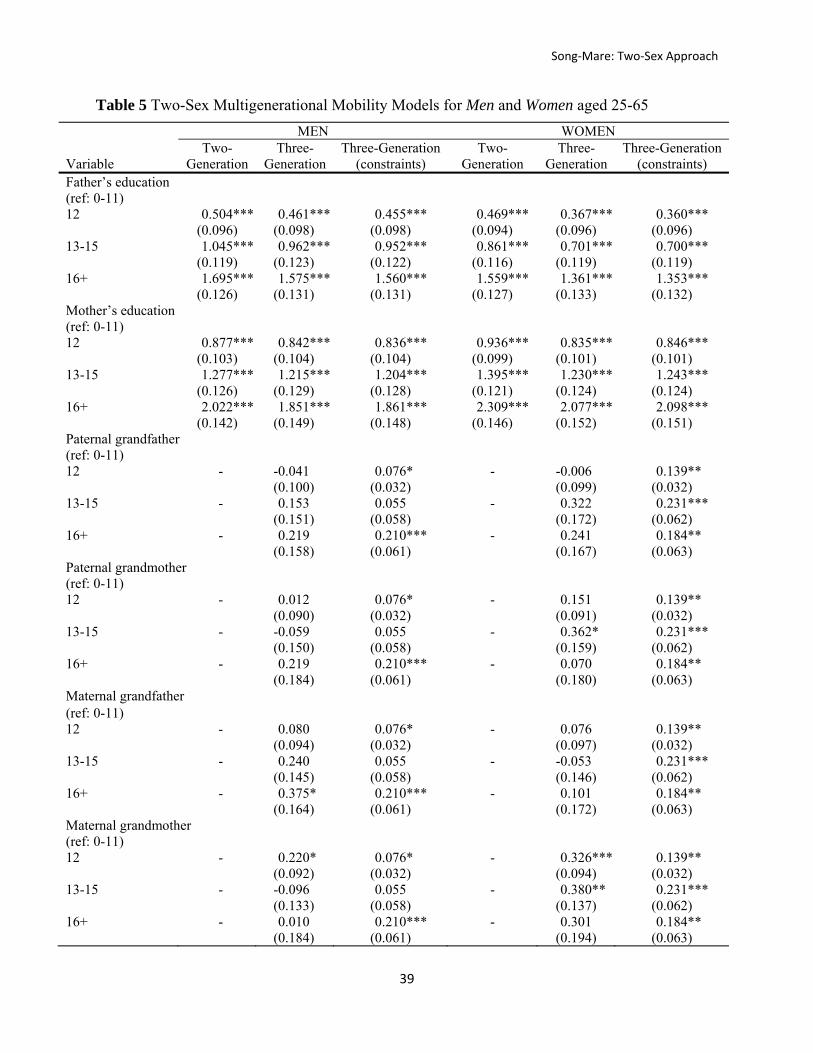
Finally, we show the two-sex mobility results from ordinal logistic regressions in Table 5.
Unlike the one-sex mobility models presented in Table 1 and 2, the two-sex models include both
parents’ and all four grandparents’ educational characteristics. We test differences between the
Song‐Mare: Two‐Sex Approach
18
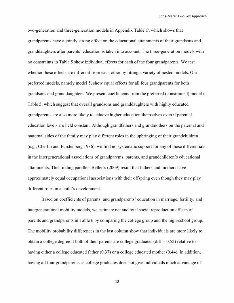
two-generation and three-generation models in Appendix Table C, which shows that
grandparents have a jointly strong effect on the educational attainments of their grandsons and
granddaughters after parents’ education is taken into account. The three-generation models with
no constraints in Table 5 show individual effects for each of the four grandparents. We test
whether these effects are different from each other by fitting a variety of nested models. Our
preferred models, namely model 5, show equal effects for all four grandparents for both
grandsons and granddaughters. We present coefficients from the preferred (constrained) model in
Table 5, which suggest that overall grandsons and granddaughters with highly educated
grandparents are also more likely to achieve higher education themselves even if parental
education levels are held constant. Although grandfathers and grandmothers on the paternal and
maternal sides of the family may play different roles in the upbringing of their grandchildren
(e.g., Cherlin and Furstenberg 1986), we find no systematic support for any of these differentials
in the intergenerational associations of grandparents, parents, and grandchildren’s educational
attainments. This finding parallels Beller’s (2009) result that fathers and mothers have
approximately equal occupational associations with their offspring even though they may play
different roles in a child’s development.
Based on coefficients of parents’ and grandparents’ education in marriage, fertility, and
intergenerational mobility models, we estimate net and total social reproduction effects of
parents and grandparents in Table 6 by comparing the college group and the high-school group.
The mobility probability differences in the last column show that individuals are more likely to
obtain a college degree if both of their parents are college graduates (diff = 0.52) relative to
having either a college educated father (0.37) or a college educated mother (0.44). In addition,
having all four grandparents as college graduates does not give individuals much advantage of

Song‐Mare: Two‐Sex Approach
19
graduating from college ( 0.062) relative to having only the paternal grandfathers as college
graduates (0.061), but it does provide a benefit relative to having only college-educated maternal
grandmothers (0.031).
The net and the total social reproduction effects of parents are smaller than the mobility
probability differences because education is negatively associated with the probability of
marriage and the level of fertility, especially when both fathers’ and mothers’ educational levels
are taken into account. The one-sex model suggests that a college father produces 0.3 more sons
in college than a high-school father, whereas the two-sex model further suggests that a couple
both with college degrees produces 0.2 more college offspring than a couple both with only high-
school degrees.
The social reproduction effects of grandparents are much smaller than those of parents.
The one-sex models for males suggest that a college grandfather and a high-school father
produce 0.06 more college sons than a high-school grandfather and a high-school father. A
college grandfather produces 0.13 more college grandsons than a high-school grandfather in total.
The effects become negative in two-sex models, suggesting that a high-school couple with all
their four parents as college graduates produces 0.026 fewer college offspring than a high-school
couple with all their four parents as high-school graduates. The main reason is that the
probability of union formation between a high-school man with college parents and a high-
school woman with college parents is smaller than that probability between a high-school man
with high-school parents and a high-school woman with high-school parents given the two-
generation assortative mating patterns shown in Appendix Table B. For the same reason, two
college couples produce 0.13 fewer college grandchildren than two high-school couples.
[Table 6]

Song‐Mare: Two‐Sex Approach
20
Taken together, compared to the one-sex models, the two-sex models reveal additional
mechanisms that create multigenerational educational inequality across families. Specifically,
characteristics of fathers and mothers as well as all four grandparents jointly determine the
parents’ union formation, fertility, and their offspring’s educational mobility. Education of all
four grandparents plays an almost equally important role in the educational mobility of their
grandsons and granddaughters. To a large extent, multigenerational educational influences from
grandparents to grandchildren are “gender-blind”—no systematic differences exist between
grandfathers and grandmothers as well as between paternal and maternal grandparents.
LONG-TERM MULTIGENERATIONAL INFLUENCES
The short-term mechanisms in the transmission of educational advantages in three
generations may affect the long-term educational reproduction of families. We examine the
eventual advantages of high-education families in producing high-education progeny compared
to those of low-education families. If a family has at least one parent holding a college degree,
compared to another family in which neither of the parents holds a college degree, what are the
differences in the number of progeny in subsequent generations who themselves have college
degrees? Our long-term multigenerational analysis relies on the marriage, fertility, and mobility
rules described above in the method section and the parameters estimated from the short-term
analyses presented in Tables 1 to 5. We simulate the educational distribution of families by
generations, and explore the evolution of educational reproduction of college- and non-college
origin families before the simulation system achieves its equilibrium.
[Figure 1]
Figure 1 presents simulation results based on one-sex and two-sex approaches for both
two-generation and three-generation models of short-term effects. We allow for patterns of
Song‐Mare: Two‐Sex Approach
21
differential marriage and net fertility in the one-sex simulation, and further incorporate
assortative mating in the two-sex simulation. The gray dashed and dotted lines represent the one-
sex, two-generation multigenerational effects for males and females respectively. The solid lines
represent results from two-sex models. All the black lines represent results that further
incorporate grandparent effects in the mating, fertility, and mobility rules. Our interest is the
relative educational reproductive success of college over non-college origin families, which is
defined as the ratio of college progeny per college family to college progeny per non-college
family. A value above 1 means that college-origin families produce more college descendants
than non-college families. As discussed earlier, due to the negative relationship between
education and fertility, educational advantages for the progeny of college families may be offset
by the lower fertility of these families.
Figure 1 reveals several important patterns. First, within the first three generations,
families that start with college education produce more college descendants than families that
start with non-college education, as the values of the ratio for all the lines are above 1. This
implies that for first-generation college families, the achievement of going to college does not
only change the educational outcomes of the present generation, but may benefit as many as
three generations ahead. Second, the ratio from one-sex models falls below 1.0 and converges to
a value between 0.6 and 1.0 over the next 5 to 10 generations, depending on the model, meaning
that fertility disadvantages of college-origin families offset their initial educational mobility
advantages, and eventually college-origin families produce fewer college-educated descendants
than non-college families. Thus the effect of being in the higher education group is negative over
the longer term because the lower fertility of this group more than offsets the mobility
advantages that they can provide their offspring in the short term. Third, comparing the gray
Song‐Mare: Two‐Sex Approach
22
lines with the black lines, we find that the long run educational reproduction of families depends
upon whether the mating, fertility, and mobility processes are Markovian (only parents’ effect) or
non-Markovian (parents’ and grandparents’ effects). Under a three-generation model, the ratio
converges to the equilibrium more slowly and reaches a lower value than under a two-generation
model. For example, for the one-sex female models, the ratio declines from 0.8 in a two-
generation model to 0.7 in a three-generation model. This result suggests that when both parents
and grandparents are involved in the educational reproduction of families, educational inequality
between college and non-college families is greater than when only parents are involved.
Moreover, this inequality is even greater when all four grandparents’ effects (the black solid line)
rather than only one grandparent effect are considered (the black dashed and dotted lines).
Finally, the two-sex results gradually converge to an equilibrium ratio equal of 1, which indicates
no long run relative educational reproduction advantages among families after roughly 17
generations. The multigenerational influences caused by a family’s initial educational status and
fertility only persist for a limited number of generations. In contrast, the one-sex approach
suggests that the ratio will be stable over time at a level that reflects net fertility differences
among education groups.
The above equilibrium results point to very different conclusions about long run effects
of socioeconomic differences among families depending on whether one adopts a one-sex or
two-sex model. To investigate the differences between the two approaches, we simulate a
combination of one-sex and two-sex mating and mobility models (shown in Table 7). For the
one-sex mating model, we assume the absence of a marriage market, and thus the number of
marriages is determined by the number and preferences of either males or females. For the two-
sex mating models, we assume three mating rules as described above: unrestricted, endogamous

Song‐Mare: Two‐Sex Approach
23
and random mating. For mobility models, we distinguish between models assuming immobility,
in which individuals always inherit their same-sex parent’s educational status, and models
assuming mobility, in which individuals’ education may be different from their parents’
education. We further divide the latter into one-sex and two-sex mobility models. The one-sex
mobility model assumes that parents only influence offspring of the same sex, whereas the two-
sex model assumes that parents influence offspring of both sexes. The one-sex and two-sex
models shown in Figure 1 refer to scenarios 10 and 2 respectively, which assume that mating and
mobility both follow two-sex or one-sex rules.
[Table 7]
[Figure 2]
Figure 2 shows that, except for scenarios 6 and 12, all models that take into account a
two-sex mating rule indicate a disappearing long run educational disparity between families,
whereas all one-sex models without a mating rule indicate a permanent disparity. In all two-sex
scenarios except scenario 6, high- and low-education origin families are connected because the
mating rule allows marriages formed between progeny from families of different educational
origins. Note that in scenario 4 and 5, when only endogamy is allowed, intermarriages between
high-education and low-education families can still happen through mobility—for example,
progeny born into low-education families achieve upward mobility and marry those from high-
education families. In scenario 6 marriages between high- and low-education origin families
never occur, as their progeny always marry within their own education groups and
intergenerational immobility precludes any intermarriage that occurs as a result of mobility.
Therefore, in the presence of intermarriage, whether explicitly permitted by the marriage rule
(scenarios 1, 2, 3, 7, 8, 9) or in subsequent generations as a result of intergenerational mobility
Song‐Mare: Two‐Sex Approach
24
(scenarios 4, 5), more and more progeny in later generations carry both high-education and low-
education origin ancestry in their background. Over generations an increasing proportion of
high-education families have low-education descendants who are also descendants of low-
education families, and vice versa. Such a trend is consistent with Bernheim and Bagwell’s
(1988) argument that intermarriages make the existence of independent, persistent family
dynasties demographically impossible. As a result, the educational distributions of progeny of
high- and low-education families become increasingly alike over generations, implying that the
educational disparities among families eventually disappear.
The two-sex approach, however, is not always superior to the one-sex approach. The one-
sex approach is still useful when the transmission of education and other social characteristics
are sex-linked. For example, social positions in a patriarchal society during China’s historical
dynasties (Lee and Campbell 1997; Lee and Wang 1999; Mare and Song 2014) and the priest
status in the ancient Jewish population (Goldstein 2008) were inherited only through male lines.
This is analogous to the inheritance of the human Y chromosome, which can only be passed
down from paternal grandfathers to fathers then to sons. Although marriages connect genealogies
of families and thus make progeny social descendants of both their paternal and maternal
families, their sex-linked characteristics are still uniquely linked to their paternal families. When
comparing descendants who carry the sex-linked characteristics from families with and without
such characteristics, we only need to count male descendants in the male line, not all social
descendants in both lines. Therefore, the one-sex model is enough to explain the evolution of
inequality in the distribution of the sex-linked characteristics between the two groups of families.
Overall, the two-sex approach is not simply an extension of the one-sex approach. The
two models imply different social rules with regard to the inheritance of social status and the

Song‐Mare: Two‐Sex Approach
25
definition of “family networks” formed by marriage. The choice of the approach involves not
only a methodological concern, but also an accurate representation of the underlying social
processes.
CONCLUSION
Our analyses of social and demographic mechanisms and their consequences for families’
educational reproduction in the United States yield two main findings. First, in our analysis of
short-term multigenerational effects, a two-sex approach provides a more adequate summary of
the influences of grandparents’ educational attainments on their grandchildren’s education. The
two-sex approach reveals influences of mothers, grandmothers, and maternal grandparents on
grandchildren’s educational outcomes, which are ignored in models that exclusively analyze
father-son or mother-daughter pairs. These results challenge the Markovian assumption in
mobility studies by showing that grandparents’ educational attainments have a direct net
association with grandchildren’s educational attainments, regardless of parents’ education. All
four grandparents’ educational attainments are associated with the attainments of their grandsons
and granddaughters to an approximately equal degree. More importantly, the two-sex approach
incorporates demographic behaviors of parents, and suggests that grandparents also influence
grandchildren’s education by influencing whether and whom the parents marry and how many
children they have.
Our analysis of long-term effects shows the circumstances under which inequalities in a
given generation may have a much more sustained impact than usually recognized in mobility
research. Relying on multigenerational simulations, we find that the one-sex and the two-sex
Song‐Mare: Two‐Sex Approach
26
approaches show similar trends within the first several generations,9 suggesting that initial
educational advantages of families may benefit as many as three generations ahead, but such
advantages are later offset by a negative fertility gradient with educational attainment. Thus,
differential fertility and social mobility jointly shape future educational distributions of progeny.
In the long run, the one-sex approach suggests that such a trend will become stable, whereas the
two-sex approach suggests that all families eventually achieve the same educational distribution
of descendants. By simulating various mating, fertility, and mobility regimes, we show that the
diverging results are explained by intermarriages between high- and low-education origin
families, which are addressed in the two-sex approach, but not the one-sex approach.
This study enriches our understanding of multigenerational inequality in several regards.
Along with several other studies (Matras 1961, 1967; Lam 1986; Mare 1997; Mare and Maralani
2006; Maralani 2013; Preston 1974), we illustrate that demography plays an important role in
creating and changing intergenerational inequality. By incorporating demographic pathways into
social mobility processes, we show that the transmission of intergenerational inequality involves
not only the inequality among those who have offspring, but also the inequality between those
who have offspring and those who do not. When one considers inequality over generations, to
grandchildren, great grandchildren, and other progeny, the role of demography becomes
cumulative. The combined analysis of demography and mobility describes the socioeconomic
reproduction of families and the social metabolism of a society.
[Figure 3]
Our analyses also link short-term mobility and demographic behaviors with the long-term
educational reproductive success of families. Whereas the short-term results suggest
9 The number of generations that the two-sex model converges to its equilibrium depends on population size. When the population size is large, it takes longer for all families to be connected to each other through marriages.

Song‐Mare: Two‐Sex Approach
27
considerable inequality in mobility opportunities in each generation, the long-term results show
an equalizing trend in educational outcomes across families. The opposing implications of the
two results suggest that future research needs to explicitly model and analyze long-term
stratification processes, rather than assume that short-term inequality necessarily leads to long-
term inequality. The demographic behaviors we consider in this study include assortative mating
and differential marriage and fertility, but future research may consider more complex
demographic strategies of families, including the duration of marriage, ages of parents at
childbearing, generation gaps between grandparents, parents, and grandchildren, childhood
family structure of each generation, and the time periods of observations (Mare 2014).
The analyses shown in this paper apply to a single country in a single historical epoch.
They focus on only a single dimension of socioeconomic achievement, educational attainment,
measured dichotomously. They use multivariate models that include a modest list of individual
and family level variables, short of the state of the art in studies that focus purely on two-
generation relationships with no attention to demographic processes or in studies that focus on a
single demographic outcome rather than its interdependence with social mobility. They do not
address the difficult problems of causal inference, which efforts to isolate true multigenerational
effects (rather than descriptive associations that may be spurious in a rigorous causal analysis).
And it is beyond the scope of this paper to specify the circumstances in which analysts should
focus exclusively on what we have termed “short-term” effects, when they should go several
generations beyond the observation span of their data, when they should examine the implied
equilibrium distributions from a short-term model, and when they should consider specific
historical effects that may disrupt the intergenerational trajectories implied by ahistorical models
alone.

Song‐Mare: Two‐Sex Approach
28
Despite these limitations, our analyses have illustrated a wide variety of possible
processes through which educational inequalities among persons in one generation may persist or
change in subsequent generations. The full set of possible types of social mobility analyses is
shown in Figure 3. The intergenerational transmission of socioeconomic advantage may be
exclusively through a direct connection between parents and offspring or, additionally, other
more remote kin such as grandparents may also exert their effects across more than one
generation. Intergenerational mobility may be essentially a one-sex process through which
family advantages are embodied in the standing of just one parent or, alternatively, both parents
may have independent effects on their children (and possibly grandchildren as well).
Intergenerational social mobility may be considered in isolation from demographic processes,
especially fertility and mortality, or we may examine how individuals affect subsequent
generations through intergenerational transmission of status combined with differential net
fertility. And finally, in considering demographic mechanisms we may regard the male and
female populations as reproducing independently via their respective one-sex marriage markets
or we may regard them as interacting populations that constrain each other and, through
assortative marriage, modify the distributions of family socioeconomic positions in successive
generations. The exemplary studies cited in taxonomy in Figure 3 show that much of our
research effort has been devoted to relatively simple models and that our empirical investigations
of multigenerational and demographic processes that govern social mobility have a long way to
go.
Song‐Mare: Two‐Sex Approach
29
REFERENCES Bartholomew, D. J. (1982). Stochastic models for social processes (third edition). New York:
Wiley.
Beller, E. (2009). Bringing intergenerational social mobility research into the twenty-first
century. American Sociological Review, 74, 507-528.
Bernheim, D. B. & Bagwell, K. (1988). Is everything neutral? Journal of Political Economy, 96,
308-338.
Blau, P. M. & Duncan, O. D. (1967). The American occupational structure. New York: Wiley.
Buchmann, C. & DiPrete, T. A. (2006). The growing female advantage in college completion:
The role of family background and academic achievement. American Sociological Review,
71, 515-541.
Caswell, H. (2001). Matrix population models: Construction, analysis, and interpretation
(second edition). Sunderland, MA: Sinauer Associates.
Chan, T. W., & Boliver, V. (2013). The grandparent’s effect in social mobility: Evidence from
British birth cohort studies. American Sociological Review, 78, 662-678.
Cherlin, A. J. & Furstenberg, F. F. (1986). The new American grandparent: A place in the family,
a life apart. New York: Basic Books.
DiPrete, T. A. & Eirich, G. M. (2006). Cumulative advantage as a mechanism for inequality: A
review of theoretical and empirical developments. Annual Review of Sociology, 32, 271-297.
Duncan, O. D. (1966). Methodological issues in the analysis of social mobility. Pp. 51-97 in N. J.
Smelser & S. M. Lipset (Ed.), Social structure and mobility in economic development.
Chicago: Aldine.
Song‐Mare: Two‐Sex Approach
30
Erikson, R. & Goldthorpe, J. H. (1992). The constant flux: A study of class mobility in industrial
societies. Oxford: Clarendon Press.
Erola, J. & Moisio, P. (2007). Social mobility over three generations in Finland, 1950-2000.
European Sociological Review, 23, 169-183.
Featherman, D. L. & Hauser, R. M. (1978). Opportunity and change. New York: Academic
Press.
Goldstein, D. B. (2008). Jacob’s legacy: A genetic view of Jewish history. New Heaven, CT:
Yale University Press.
Goodman, L. A. (1953). Population growth of the sexes. Biometrics, IX, 212-225.
Hertel, F. R., & Groh-Samberg, O. (2014). Class mobility across three generations in the U.S and
Germany. Research in Social Stratification and Mobility, 35, 35-52.
Hodge, R. W. (1966). Occupational mobility as a probability process. Demography, 3, 19–34.
Hout, M. (1983). Mobility tables. Beverly Hills, CA: Sage Publications.
Hout, M. (1988). More universalism, less structural mobility: The American occupational
structure in the 1980s. American Journal of Sociology, 93, 1358-1400.
Jæger, M. M. (2012). The extended family and children’s educational success. American
Sociological Review, 77, 903-922.
Keyfitz, N. (1968). Introduction to the mathematics of population. Addison-Wesley Publishing
Company.
Keyfitz, N. (1972). The mathematics of sex and marriage. Proceedings of the Sixth Berkeley
Symposium on Mathematical Statistics and Probability, 4, 89-108.
Lam, D. (1986). The dynamics of population growth, differential fertility, and inequality.
American Economic Review, 76, 1103-1116.
Song‐Mare: Two‐Sex Approach
31
Lee, J. Z., & Campbell, C. D. (1997). Fate and fortune in rural China: Social organization and
population behavior in Liaoning, 1774-1873. Cambridge University Press.
Lee, J. Z., & Wang, F. (1999). One quarter of humanity: Malthusian mythology and Chinese
realities, 1700-2000. Harvard University Press.
Maralani, V. (2013). The demography of social mobility: Black-white differences in educational
reproduction. American Journal of Sociology, 118, 1509-1558.
Mare, R. D. (1997). Differential fertility, intergenerational educational mobility, and racial
inequality. Social Science Research, 26, 263–291.
Mare, R. D. (2000). Assortative mating, intergenerational mobility, and educational inequality.
Working paper CCPR-004-00 UCLA California Center for Population Research
Mare, R. D. (2011). A multigenerational view of inequality. Demography, 48, 1-23.
Mare, R. D. (2014). Multigenerational aspects of social stratification: Issues for future research.
Research in Social Stratification and Mobility, 35, 121-128.
Mare, R. D., & Schwartz, C. R. (2006). Educational assortative mating and the family
background of the next generation: A formal analysis. Riron to Hoho (Sociological Theory
and Methods), 21, 253–277.
Mare, R. D., & Maralani, V. (2006). The intergenerational effects of changes in women’s
educational attainments. American Sociological Review, 71, 542-564.
Mare, R. D., & Song, X. (2014). Social mobility in multiple generations. Unpublished
manuscript. Los Angeles. California Center for Population Research.
Matras, J. (1961). Differential fertility, intergenerational occupational mobility and change in the
occupational distribution: Some elementary interrelationships. Population Studies, 15, 187-
197.
Song‐Mare: Two‐Sex Approach
32
Matras, J. (1967). Social mobility and social structure: Some insights from the linear model.
American Sociological Review, 32, 608-614.
Pfeffer, F. (2014). Multigenerational approaches to social mobility: A multifaceted research
agenda. Research in Social Stratification and Mobility, 35, 1-12.
Pollak, R. A. (1986). A reformulation of the two-sex problem. Demography, 23, 247-259.
Pollak, R. A. (1987). The two-sex problem with persistent unions: A generalization of the birth
matrix-mating rule model. Theoretical Population Biology, 32, 176-187.
Pollak, R. A. (1990). Two-sex demographic models. Journal of Political Economy, 98, 399-420.
Preston, S. H. (1974). Differential fertility, unwanted fertility, and racial trends in occupational
achievement. American Sociological Review, 39, 492-506.
Preston, S. H., & Campbell, C. D. (1993). Differential fertility and the distribution of traits: The
case of IQ. American Journal of Sociology, 98, 997-1019.
PSID Main Interview User Manual: Release 2013. Institute for Social Research, University of
Michigan, July, 2013.
Qian, Z., & Preston, S. H. (1993). Changes in American marriage, 1972 to 1987: Availability
and forces of attraction by age and education. American Sociological Review, 58, 482-495.
Schoen, R. (1981). The harmonic mean as the basis of a realistic two-sex marriage model.
Demography, 18, 201-216.
Schoen, R. (1988). Modeling multigroup populations. New York: Plenum.
Sewell, W. H. & Hauser, R. M. (1975). Education, occupation, and earnings: Achievement in the
early career. New York: Academic Press.

Song‐Mare: Two‐Sex Approach
33
Warren, J. R., & Hauser, R. M. (1997). Social stratification across three generations: New
evidence from the Wisconsin Longitudinal Study. American Sociological Review, 62, 561-
572.
Wightman, P., & Danziger, S. (2014). Multigenerational income disadvantage and the
educational attainment of young adults. Research in Social Stratification and Mobility, 35,
53-69.
Zeng, Z., & Xie, Y. (2014). The effects of grandparents on children’s schooling: Evidence from
rural China. Demography, 51, 599-617.
Song‐Mare: Two‐Sex Approach
34
Table 1 One-Sex Multigenerational Marriage, Fertility, and Mobility Models for Men
Marriage Marital Fertility Mobility
Ever Married (Logit)
Children Ever Born (Negative binomial)
Son’s Education (Ordered logit)
Variable 2 Generation 3 Generation 2 Generation 3 Generation 2 Generation 3 Generation Men’s education (ref: 0-11)
12 0.414*** (0.074)
0.385*** (0.076)
-0.169*** (0.024)
-0.156*** (0.025)
- -
13-15 0.595*** (0.083)
0.564*** (0.087)
-0.268*** (0.027)
-0.243*** (0.029)
- -
16+ 0.837*** (0.090)
0.811*** (0.100)
-0.358*** (0.029)
-0.321*** (0.031)
- -
Father’s education (ref: 0-11)
12 - 0.118 (0.067)
- -0.037 (0.021)
0.922*** (0.089)
0.874*** (0.090)
13-15 - 0.073 (0.092)
- -0.053 (0.032)
1.667*** (0.109)
1.564*** (0.112)
16+ - 0.050 (0.093)
- -0.077* (0.031)
2.681*** (0.108)
2.525*** (0.113)
Paternal grandfather (ref: 0-11) 12 - - - - - 0.163
(0.088) 13-15 - - - - - 0.384**
(0.144) 16+ - - - - - 0.544***
(0.141) Age group (ref: 25-35) 36-45 1.054***
(0.071) 1.060***
(0.072) 0.137***
(0.035) 0.133***
(0.035) - -
46-55 1.453*** (0.067)
1.474*** (0.070)
0.200*** (0.032)
0.188*** (0.032)
- -
56-65 2.452*** (0.089)
2.483*** (0.093)
0.378*** (0.031)
0.359*** (0.032)
- -
Intercept -0.365*** (0.079)
-0.415*** (0.085)
0.658*** (0.035)
0.681*** (0.036)
-
Cut Point 1 - - - - -1.059*** (0.073)
-1.038*** (0.073)
Cut Point 2 - - - - 1.222*** (0.074)
1.248*** (0.075)
Cut Point 3 - - - - 2.576*** (0.084)
2.609*** (0.085)
N 9,683 9,683 6,869 6,869 3,122 3,122 Log-likelihood -4540.0 -4538.4 -11480.6 -11476.9 -3741.3 -3731.1
Data source: The Panel Study of Income Dynamics 1968-2011. Notes: ***p< 0.001; **p< 0.01; *p< 0.05. Preferred models are highlighted.

Song‐Mare: Two‐Sex Approach
35
Table 2 One-Sex Multigenerational Marriage, Fertility, and Mobility Models for Women
Marriage Marital Fertility Mobility Ever Married
(Logit) Children Ever Born (Negative binomial)
daughter’s Education (Ordered logit)
Variable 2 Generation 3 Generation 2 Generation 3 Generation 2 Generation 3 Generation Women’s education (ref: 0-11)
12 0.515*** (0.081)
0.423*** (0.083)
-0.240*** (0.024)
-0.224*** (0.025)
- -
13-15 0.708*** (0.089)
0.579*** (0.094)
-0.330*** (0.027)
-0.309*** (0.029)
- -
16+ 0.792*** (0.094)
0.650*** (0.103)
-0.490*** (0.029)
-0.461*** (0.032)
- -
Mother’s education (ref: 0-11)
12 - 0.351*** (0.072)
- -0.050* (0.020)
1.265*** (0.091)
1.111*** (0.094)
13-15 - 0.308*** (0.091)
- -0.011 (0.028)
2.021*** (0.107)
1.787*** (0.112)
16+ - 0.258** (0.105)
- -0.069* (0.034)
3.225*** (0.127)
2.901*** (0.134)
Maternal grandmother (ref: 0-11) - - - - - - 12 - - - - - 0.544***
(0.081) 13-15 - - - - - 0.528***
(0.126) 16+ - - - - - 0.701***
(0.171) Age group (ref: 25-35) 36-45 1.108***
(0.075) 1.127**
(0.076) 0.157***
(0.033) 0.155***
(0.033) - -
46-55 1.607*** (0.072)
1.678*** (0.075)
0.199*** (0.030)
0.192*** (0.031)
- -
56-65 2.270*** (0.091)
2.369*** (0.094)
0.255*** (0.031)
0.245*** (0.032)
- -
Intercept -0.214*** (0.085)
-0.375*** (0.092)
0.818*** (0.034)
0.836*** (0.036)
- -
Cut Point 1 - - - - -1.264*** (0.079)
-1.210*** (0.079)
Cut Point 2 - - - - 1.239*** (0.078)
1.313 (0.080)
Cut Point 3 - - - - 2.597*** (0.088)
2.693*** (0.089)
N 9,867 9,867 6,802 6,802 3,145 3,145 Log-likelihood -4202.6 -4190.2 -11073.8 -11069.8 -3651.6 -3622.9
Data source: The Panel Study of Income Dynamics 1968-2011. Notes: ***p< 0.001; **p< 0.01; *p< 0.05. Preferred models based on likelihood ratio tests are highlighted.
Song‐Mare: Two‐Sex Approach
36
Table 3 Two-Sex Assortative Mating and Force of Attraction
Panel A Observed Assortative Mating Schooling Men
Women
# of eligible males
(age 25-65)
# of eligible females
(age 25-65)
# of eligible male person-year (age 25-65)
# of eligible female person-year (age 25-65)
# of marriages
Force of attraction ( )
0-11 0-11 1,534 1,466 17,314 12,781 451 0.061 12 1,534 3,846 17,314 28,872 493 0.046 13-15 1,534 2,484 17,314 20,108 119 0.013 16+ 1,534 2,017 17,314 19,329 28 0.003 12 0-11 3,872 1,466 38,730 12,781 379 0.039 12 3,872 3,846 38,730 28,872 1,478 0.089 13-15 3,872 2,484 38,730 20,108 658 0.050 16+ 3,872 2,017 38,730 19,329 239 0.019 13-15 0-11 2,317 1,466 23,609 12,781 96 0.012 12 2,317 3,846 23,609 28,872 568 0.044 13-15 2,317 2,484 23,609 20,108 671 0.062 16+ 2,317 2,017 23,609 19,329 349 0.033 16+ 0-11 1,860 1,466 19,585 12,781 20 0.003 12 1,860 3,846 19,585 28,872 210 0.018 13-15 1,860 2,484 19,585 20,108 355 0.036 16+ 1,860 2,017 19,585 19,329 883 0.091 Total Total 9,583 9,813 99,238 81,090 6,992 -
Data source: The Panel Study of Income Dynamics 1968-2011. Notes: The expected number of eligible person years = average age at marriage (for the married) * the number of married + (60-18) * # of unmarried.

Song‐Mare: Two‐Sex Approach
37
Table 4 Two-Sex Multigenerational Marriage and Fertility Models for Men and Women
Marriage Marriage Marital Fertility Men Ever Married
(Logit) Women Ever Married
(Logit) Couples
(Negative binomial) Variable 2 Generation 3 Generation 2 Generation 3 Generation 2 Generation 3 Generation Men’s education (ref: 0-11)
12 0.414*** (0.074)
0.378*** (0.077)
- - -0.111*** (0.018)
-0.096*** (0.018)
13-15 0.595*** (0.083)
0.572*** (0.089)
- - -0.155*** (0.021)
-0.132*** (0.022)
16+ 0.837*** (0.090)
0.827*** (0.103)
- - -0.207*** (0.024)
-0.172*** (0.026)
Women’s education (ref: 0-11)
12 - - 0.515*** (0.081)
0.396*** (0.084)
-0.152*** (0.018)
-0.139*** (0.019)
13-15 - - 0.708*** (0.089)
0.535*** (0.095)
-0.196*** (0.021)
-0.180*** (0.022)
16+ - - 0.792*** (0.094)
0.553*** (0.106)
-0.285*** (0.025)
-0.264*** (0.026)
Men’s father (ref: 0-11)
12 ‐ 0.090 (0.073)
‐ ‐ ‐ 0.017 (0.017)
13-15 ‐ 0.106 (0.099)
‐ ‐ ‐ 0.007 (0.024)
16+ ‐ 0.090 (0.103)
‐ ‐ ‐ -0.014 (0.025)
Men’s mother (ref: 0-11) 12 - 0.105
(0.075) - - - -0.053**
(0.017) 13-15 - -0.140
(0.095) - - - -0.056*
(0.024) 16+ - -0.070
(0.110) - - - -0.051
(0.027) Women’s father (ref: 0-11) 12 - - - 0.181*
(0.076) - -0.031
(0.017) 13-15 - - - 0.182
(0.099) - -0.048*
(0.023) 16+ - - - 0.465***
(0.111) - -0.031
(0.024) Women’s mother (ref: 0-11) 12
- - - 0.269***
(0.078) - -0.010
(0.017) 13-15
- - - 0.189
(0.098) - 0.056*
(0.022) 16+ -
- - 0.040
(0.117) - -0.016
(0.027)

Song‐Mare: Two‐Sex Approach
38
Table 4 (continued)
Marriage Marriage Marital Fertility Men Ever Married
(Logit) Women Ever Married
(Logit)Couples
(Negative binomial) 2 Generation 3 Generation 2 Generation 3 Generation 2 Generation 3 Generation Age group (ref: 25-35) 36-45 1.054***
(0.071) 1.050***
(0.072) 1.108***
(0.075) 1.127***
(0.076) 0.153***
(0.024) 0.148***
(0.024) 46-55 1.453***
(0.067) 1.457***
(0.070) 1.607***
(0.072) 1.708***
(0.076) 0.193***
(0.022) 0.181***
(0.023) 56-65 2.452***
(0.089) 2.468***
(0.094) 2.270***
(0.091) 2.407***
(0.096) 0.304***
(0.022) 0.285***
(0.023) Intercept -0.365***
(0.079) -0.417*** (0.089)
-0.214* (0.085)
-0.424*** (0.094)
0.797*** (0.026)
0.824*** (0.028)
N 9,683 9,683 9,867 9,867 13,311 13,311 Log-likelihood -4540.0 -4533.1 -4202.6 -4181.2 -21944.9 -21927.1
Data source: The Panel Study of Income Dynamics 1968-2011. Notes: ***p< 0.001; **p< 0.01; *p< 0.05.
Song‐Mare: Two‐Sex Approach
39
Table 5 Two-Sex Multigenerational Mobility Models for Men and Women aged 25-65
MEN WOMEN Variable
Two-Generation
Three-Generation
Three-Generation (constraints)
Two-Generation
Three-Generation
Three-Generation (constraints)
Father’s education (ref: 0-11)
12
0.504*** (0.096)
0.461***(0.098)
0.455*** (0.098)
0.469*** (0.094)
0.367*** (0.096)
0.360*** (0.096)
13-15 1.045*** (0.119)
0.962***(0.123)
0.952*** (0.122)
0.861*** (0.116)
0.701*** (0.119)
0.700*** (0.119)
16+ 1.695*** (0.126)
1.575***(0.131)
1.560*** (0.131)
1.559*** (0.127)
1.361*** (0.133)
1.353*** (0.132)
Mother’s education (ref: 0-11)
12 0.877*** (0.103)
0.842***(0.104)
0.836*** (0.104)
0.936*** (0.099)
0.835*** (0.101)
0.846*** (0.101)
13-15 1.277*** (0.126)
1.215***(0.129)
1.204*** (0.128)
1.395*** (0.121)
1.230*** (0.124)
1.243*** (0.124)
16+ 2.022*** (0.142)
1.851***(0.149)
1.861*** (0.148)
2.309*** (0.146)
2.077*** (0.152)
2.098*** (0.151)
Paternal grandfather (ref: 0-11) 12 -
-0.041 (0.100)
0.076* (0.032)
- -0.006 (0.099)
0.139** (0.032)
13-15 -
0.153 (0.151)
0.055 (0.058)
- 0.322 (0.172)
0.231*** (0.062)
16+ -
0.219 (0.158)
0.210*** (0.061)
- 0.241 (0.167)
0.184** (0.063)
Paternal grandmother (ref: 0-11) 12 -
0.012
(0.090) 0.076*
(0.032) - 0.151
(0.091) 0.139**
(0.032) 13-15 -
-0.059 (0.150)
0.055 (0.058)
- 0.362* (0.159)
0.231*** (0.062)
16+ -
0.219 (0.184)
0.210*** (0.061)
- 0.070 (0.180)
0.184** (0.063)
Maternal grandfather (ref: 0-11) 12 -
0.080
(0.094) 0.076*
(0.032) - 0.076
(0.097) 0.139**
(0.032) 13-15 -
0.240
(0.145) 0.055
(0.058) - -0.053
(0.146) 0.231***
(0.062) 16+ -
0.375*
(0.164) 0.210***
(0.061) - 0.101
(0.172) 0.184**
(0.063) Maternal grandmother (ref: 0-11) 12 -
0.220*
(0.092) 0.076*
(0.032) - 0.326***
(0.094) 0.139**
(0.032) 13-15 -
-0.096 (0.133)
0.055 (0.058)
- 0.380** (0.137)
0.231*** (0.062)
16+ - 0.010 (0.184)
0.210*** (0.061)
- 0.301 (0.194)
0.184** (0.063)
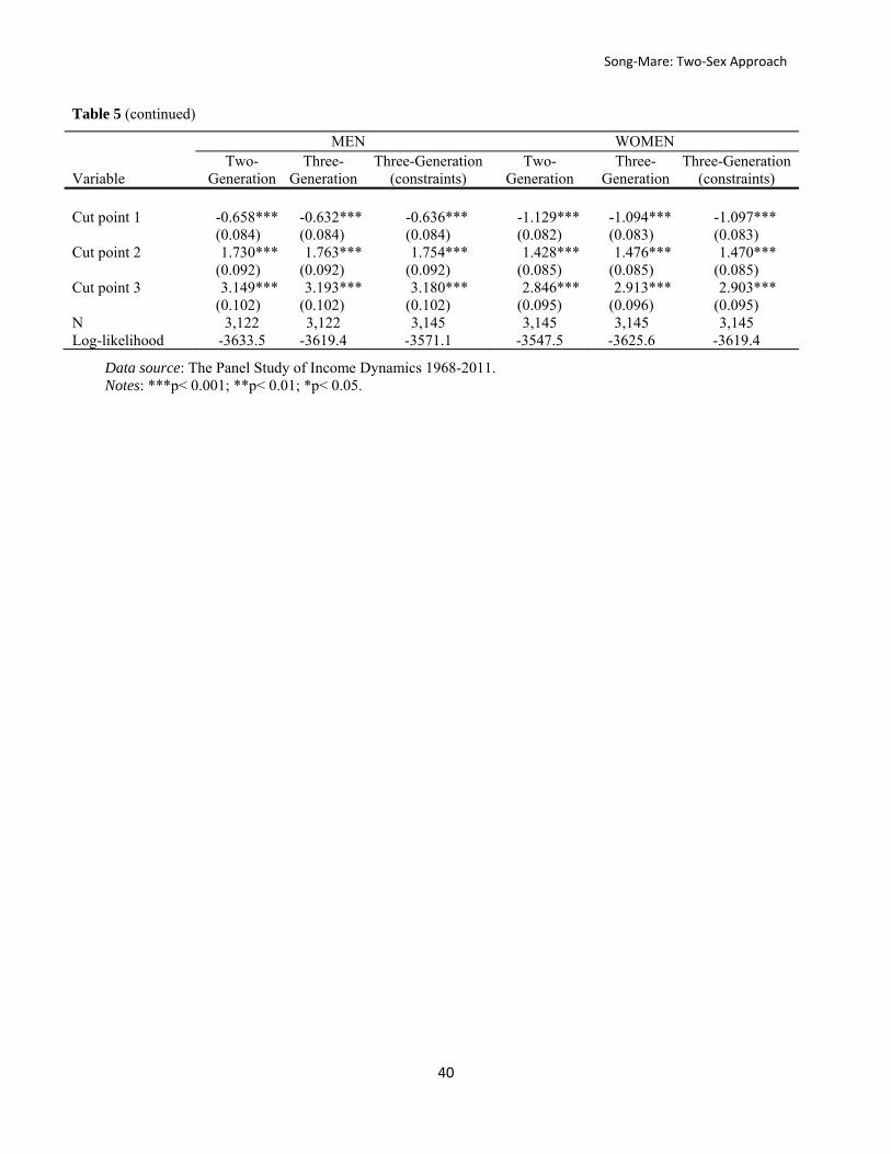
Song‐Mare: Two‐Sex Approach
40
Table 5 (continued)
MEN WOMEN
Variable
Two-Generation
Three-Generation
Three-Generation (constraints)
Two-Generation
Three-Generation
Three-Generation (constraints)
Cut point 1 -0.658***
(0.084) -0.632***(0.084)
-0.636*** (0.084)
-1.129*** (0.082)
-1.094*** (0.083)
-1.097*** (0.083)
Cut point 2 1.730*** (0.092)
1.763***(0.092)
1.754*** (0.092)
1.428*** (0.085)
1.476*** (0.085)
1.470*** (0.085)
Cut point 3 3.149*** (0.102)
3.193***(0.102)
3.180*** (0.102)
2.846*** (0.095)
2.913*** (0.096)
2.903*** (0.095)
N 3,122 3,122 3,145 3,145 3,145 3,145 Log-likelihood -3633.5 -3619.4 -3571.1 -3547.5 -3625.6 -3619.4
Data source: The Panel Study of Income Dynamics 1968-2011. Notes: ***p< 0.001; **p< 0.01; *p< 0.05.

Song‐Mare: Two‐Sex Approach
41
Table 6 Short-Term Net and Total Social Reproduction Effects
Social Reproduction Effect Mobility probability differences Net effect Total effect
Parents One-sex (father) 0.315 0.315 0.366 One-sex (mother) 0.329 0.329 0.443 Two-sex 0.224 0.224 0.518 Grandparents One-sex (grandfather) 0.055 0.131 0.061 One-sex (grandmother) 0.026 0.046 0.031 Two-sex -0.026 -0.132 0.062
Data source: The Panel Study of Income Dynamics 1968-2011. Notes: For the net social reproduction effect, we compare parents (or grandparents) who are college graduates to those who are high-school graduates in producing college offspring. For the total net effect of grandparents, we compare grandparents who are college graduates to those who are high-school graduates in producing college grandchildren. For the mobility probability differences, we calculate the difference between the probability of attaining college by having college parents rather than high-school parents (or college grandparents and high school parents vs. high-school grandparents and parents). These figures are calculated based on equations (4), (5), (9), and (10).
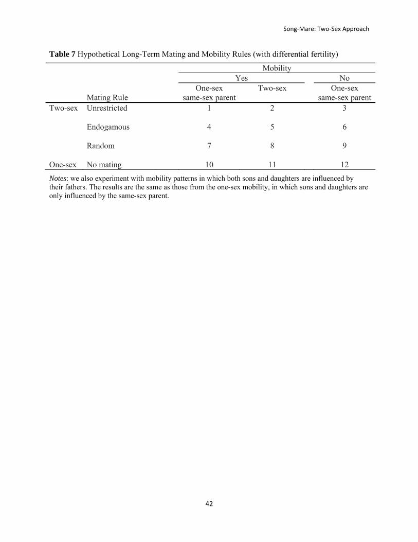
Song‐Mare: Two‐Sex Approach
42
Table 7 Hypothetical Long-Term Mating and Mobility Rules (with differential fertility)
Mobility Yes No One-sex Two-sex One-sex Mating Rule same-sex parent same-sex parent Two-sex Unrestricted
1 2 3
Endogamous
4 5 6
Random 7 8 9 One-sex No mating 10 11 12
Notes: we also experiment with mobility patterns in which both sons and daughters are influenced by their fathers. The results are the same as those from the one-sex mobility, in which sons and daughters are only influenced by the same-sex parent.

Song‐Mare: Two‐Sex Approach
43
Fig 1. Multigenerational Reproduction of College Education
Notes: We define the effect as the ratio of college progeny per college family over college progeny per non-college family. The ratio = 1 means no multigenerational effect.
0.0
0.5
1.0
1.5
2.0
2.5
3.0
1 2 3 4 5 6 7 8 9 10 11 12 13 14 15 16 17 18 19 20
Eff
ect
Synthetic Generations
1-sex, 2-generation, male 1-sex, 3-generation, male 1-sex, 2-generation, female
1-sex, 3-generation, female 2-sex, 2-generation 2-sex, 3-generation
(no effect)
One-sex long-term multigenerational effect
Two-sex long-term multigenerational effect

Song‐Mare: Two‐Sex Approach
44
Fig 2. Multigenerational Reproduction of College Education based on Various Scenarios of Mating and Mobility Rules
Notes: We define the effect as the ratio of college progeny per college family over college progeny per non-college family.
0
1
2
3
4
5
6
7
8
9
10
0 1 2 3 4 5 6 7 8 9 10 11 12 13 14 15 16 17 18 19 20
Eff
ect
Synthetic Generations
1 unrestricted, one-sex mobility 2 unrestricted, two-sex mobility
3 unrestricted, immobility 4 endogamy, one-sex mobility
5 endogamy, two-sex mobility 6 endogamy, immobility
7 random, one-sex mobility 8 random, two-sex mobility
9 random, immobility 10 no mating, one-sex mobility
11 no mating, two-sex mobility 12 no mating, immobility
No effect: 1, 2, 3, 4, 5, 7, 8, 9
Permanent effect: 10, 11
∞ 6 12
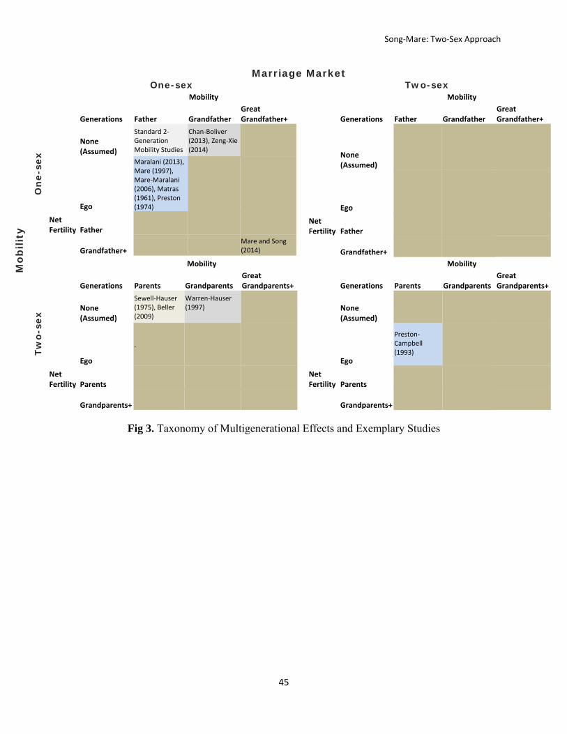
Song‐Mare: Two‐Sex Approach
45
Marriage Market One-sex Two-sex
Mo
bili
ty
On
e-se
x
Mobility
Generations Father Grandfather Great Grandfather+
None (Assumed)
Standard 2‐Generation Mobility Studies
Chan‐Boliver (2013), Zeng‐Xie (2014)
Ego
Maralani (2013), Mare (1997), Mare‐Maralani (2006), Matras (1961), Preston (1974)
Net Fertility Father
Grandfather+
Mare and Song (2014)
Mobility
Generations Father Grandfather Great Grandfather+
None (Assumed)
Ego
Net Fertility Father
Grandfather+
Two-
sex
Mobility
Generations Parents Grandparents Great Grandparents+
None (Assumed)
Sewell‐Hauser (1975), Beller (2009)
Warren‐Hauser (1997)
Ego
.
Net Fertility Parents
Grandparents+
Mobility
Generations Parents Grandparents Great Grandparents+
None (Assumed)
Ego
Preston‐Campbell (1993)
Net Fertility Parents
Grandparents+
Fig 3. Taxonomy of Multigenerational Effects and Exemplary Studies
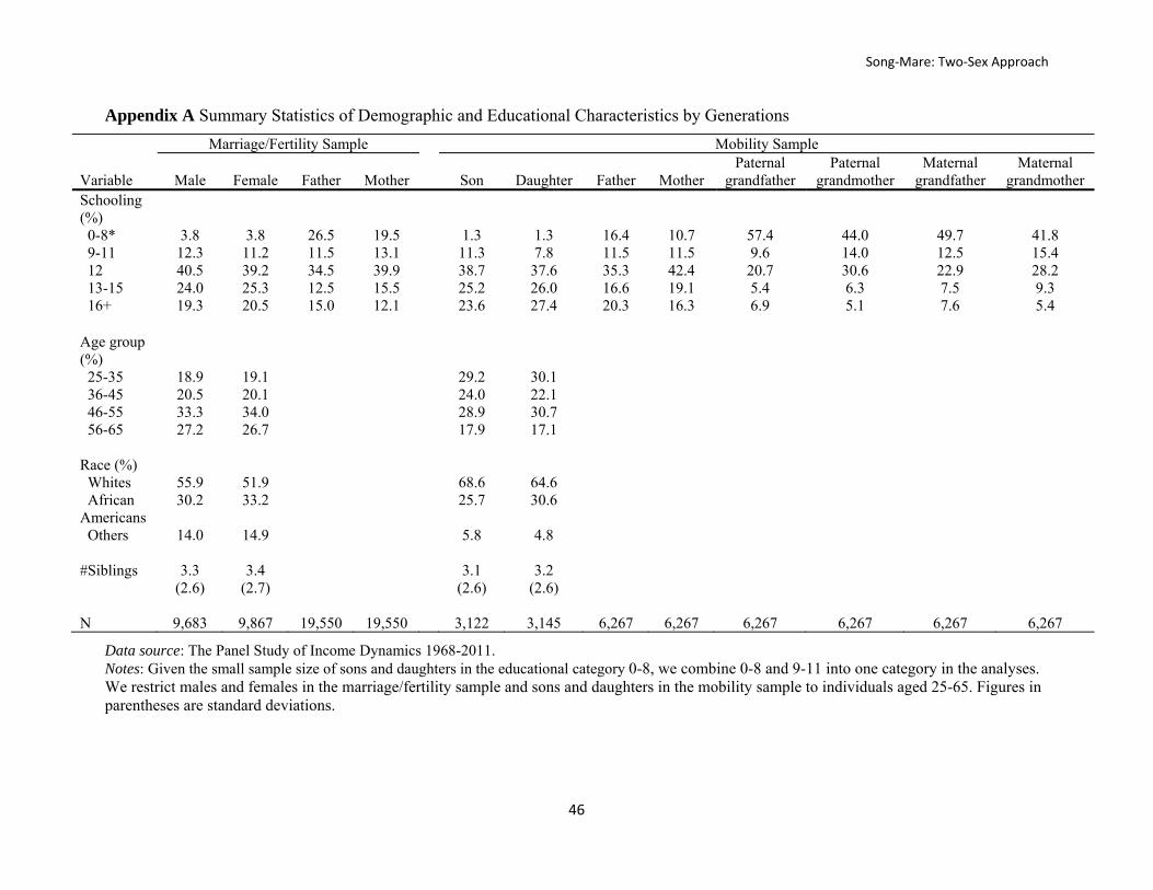
Song‐Mare: Two‐Sex Approach
46
Appendix A Summary Statistics of Demographic and Educational Characteristics by Generations
Marriage/Fertility Sample Mobility Sample Variable
Male
Female
Father
Mother
Son
Daughter
Father
Mother
Paternal grandfather
Paternal grandmother
Maternal grandfather
Maternal grandmother
Schooling (%)
0-8* 3.8 3.8 26.5 19.5 1.3 1.3 16.4 10.7 57.4 44.0 49.7 41.8 9-11 12.3 11.2 11.5 13.1 11.3 7.8 11.5 11.5 9.6 14.0 12.5 15.4 12 40.5 39.2 34.5 39.9 38.7 37.6 35.3 42.4 20.7 30.6 22.9 28.2 13-15 24.0 25.3 12.5 15.5 25.2 26.0 16.6 19.1 5.4 6.3 7.5 9.3 16+ 19.3 20.5 15.0 12.1 23.6 27.4 20.3 16.3 6.9 5.1 7.6 5.4 Age group (%)
25-35 18.9 19.1 29.2 30.1 36-45 20.5 20.1 24.0 22.1 46-55 33.3 34.0 28.9 30.7 56-65 27.2 26.7 17.9 17.1
Race (%) Whites 55.9 51.9 68.6 64.6 African Americans
30.2 33.2 25.7 30.6
Others
14.0 14.9 5.8 4.8
#Siblings 3.3 (2.6)
3.4 (2.7)
3.1 (2.6)
3.2 (2.6)
N 9,683 9,867 19,550 19,550 3,122 3,145 6,267 6,267 6,267 6,267 6,267 6,267
Data source: The Panel Study of Income Dynamics 1968-2011. Notes: Given the small sample size of sons and daughters in the educational category 0-8, we combine 0-8 and 9-11 into one category in the analyses. We restrict males and females in the marriage/fertility sample and sons and daughters in the mobility sample to individuals aged 25-65. Figures in parentheses are standard deviations.
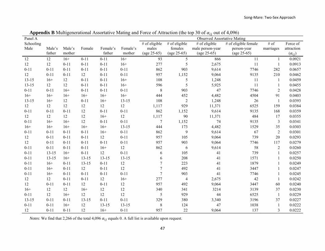
Song‐Mare: Two‐Sex Approach
47
Appendix B Multigenerational Assortative Mating and Force of Attraction (the top 30 of out of 4,096) Panel A Observed Assortative Mating Schooling Male
Male’s father
Male’s mother
Female
Female’s
father
Female’s mother
# of eligible males
(age 25-65)
# of eligible females
(age 25-65)
# of eligible male person-year
(age 25-65)
# of eligible female person-year (age 25-65)
# of marriages
Force of attraction
( )
12 12 16+ 0-11 0-11 16+ 93 5 866 11 1 0.0921 12 12 0-11 0-11 0-11 16+ 277 5 2,675 11 1 0.0913 0-11 0-11 0-11 0-11 0-11 0-11 862 903 9,614 7746 282 0.0657 12 0-11 0-11 12 0-11 0-11 957 1,152 9,064 9135 210 0.0462 13-15 16+ 12 0-11 0-11 16+ 108 5 1,248 11 1 0.0459 13-15 12 12 0-11 0-11 16+ 596 5 5,925 11 1 0.0455 0-11 0-11 16+ 0-11 0-11 0-11 8 903 47 7746 2 0.0428 16+ 16+ 16+ 16+ 16+ 16+ 444 452 4,482 4504 91 0.0403 13-15 16+ 12 0-11 16+ 13-15 108 2 1,248 26 1 0.0393 12 12 12 12 12 12 1,117 929 11,371 6525 159 0.0384 0-11 0-11 0-11 12 0-11 0-11 862 1,152 9,614 9135 168 0.0359 12 12 12 12 16+ 12 1,117 90 11,371 484 17 0.0355 0-11 16+ 16+ 12 0-11 0-11 7 1,152 74 9135 3 0.0341 16+ 16+ 16+ 16+ 16+ 13-15 444 173 4,482 1529 35 0.0303 0-11 0-11 0-11 0-11 16+ 0-11 862 9 9,614 67 2 0.0301 12 0-11 0-11 0-11 12 0-11 957 105 9,064 739 20 0.0293 12 0-11 0-11 0-11 0-11 0-11 957 903 9,064 7746 117 0.0279 0-11 0-11 0-11 0-11 16+ 12 862 6 9,614 58 2 0.0260 0-11 13-15 16+ 0-11 12 0-11 6 105 41 739 1 0.0257 0-11 13-15 16+ 13-15 13-15 13-15 6 208 41 1571 1 0.0250 0-11 16+ 0-11 13-15 0-11 12 7 223 41 1879 1 0.0249 0-11 16+ 0-11 12 0-11 12 7 492 41 3447 1 0.0247 0-11 16+ 0-11 0-11 0-11 0-11 7 903 41 7746 1 0.0245 12 12 0-11 0-11 12 16+ 277 4 2,675 42 1 0.0242 12 0-11 0-11 12 0-11 12 957 492 9,064 3447 60 0.0240 16+ 12 12 16+ 12 12 340 341 3214 3139 37 0.0230 0-11 12 16+ 12 12 12 5 929 44 6525 1 0.0229 13-15 0-11 0-11 13-15 0-11 0-11 329 380 3,340 3196 37 0.0227 0-11 0-11 16+ 12 13-15 13-15 8 124 47 1038 1 0.0222 12 0-11 0-11 12 16+ 0-11 957 22 9,064 137 3 0.0222
Notes: We find that 2,266 of the total 4,096 equals 0. A full list is available upon request.
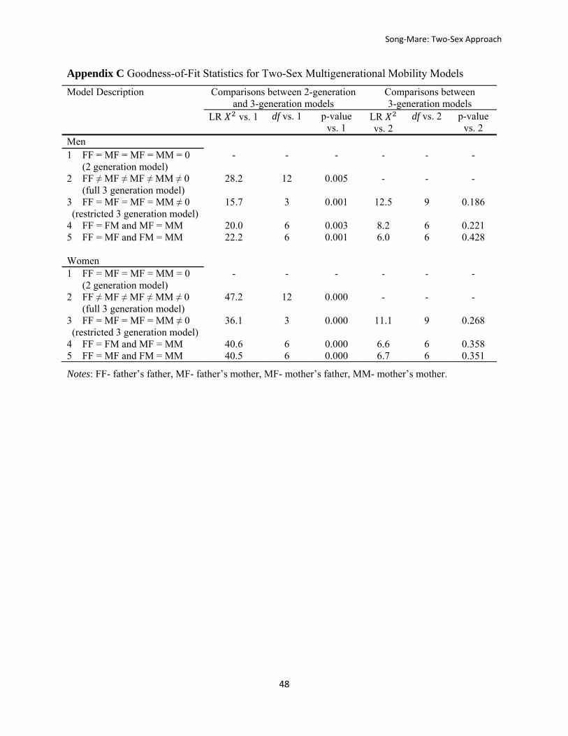
Song‐Mare: Two‐Sex Approach
48
Appendix C Goodness-of-Fit Statistics for Two-Sex Multigenerational Mobility Models
Model Description Comparisons between 2-generation and 3-generation models
Comparisons between 3-generation models
LR vs. 1 df vs. 1 p-value vs. 1
LR vs. 2
df vs. 2 p-value vs. 2
Men 1 FF = MF = MF = MM = 0 (2 generation model)
- - - ‐ ‐ -
2 FF ≠ MF ≠ MF ≠ MM ≠ 0 (full 3 generation model)
28.2 12 0.005 - - -
3 FF = MF = MF = MM ≠ 0 (restricted 3 generation model)
15.7 3 0.001 12.5 9 0.186
4 FF = FM and MF = MM 20.0 6 0.003 8.2 6 0.221 5 FF = MF and FM = MM 22.2 6 0.001 6.0 6 0.428 Women 1 FF = MF = MF = MM = 0 (2 generation model)
- - - ‐ ‐ -
2 FF ≠ MF ≠ MF ≠ MM ≠ 0 (full 3 generation model)
47.2 12 0.000 - - -
3 FF = MF = MF = MM ≠ 0 (restricted 3 generation model)
36.1 3 0.000 11.1 9 0.268
4 FF = FM and MF = MM 40.6 6 0.000 6.6 6 0.358 5 FF = MF and FM = MM 40.5 6 0.000 6.7 6 0.351
Notes: FF- father’s father, MF- father’s mother, MF- mother’s father, MM- mother’s mother.