short introduction to climate change modellingusers.auth.gr/vmarios/erasmus/short introduction to...
TRANSCRIPT

18/10/18Marios VafiadisDIVISION OF HYDRAULICS AND ENVIRONMENTAL ENGINEERING
Short Introduction to Climate Change Modelling

18/10/18Marios VafiadisDIVISION OF HYDRAULICS AND ENVIRONMENTAL ENGINEERING
http://www.ipcc.ch/

18/10/18Marios VafiadisDIVISION OF HYDRAULICS AND ENVIRONMENTAL ENGINEERING

18/10/18Marios VafiadisDIVISION OF HYDRAULICS AND ENVIRONMENTAL ENGINEERING
Atmospheric circulation
Wikipedia

18/10/18Marios VafiadisDIVISION OF HYDRAULICS AND ENVIRONMENTAL ENGINEERING
A General Circulation Model (GCM) is a mathematical model of the general circulation of the Earth’s atmosphere based on the Navier-Stokes equations on a rotating sphere with thermodynamic terms for various energy sources (radiation, latent heat). Sea-ice and land-surface components can be also combined with GCM in order to provide a more complete Global climate model.
These equations are the basis for complex computer programs commonly used for simulating the atmosphere or ocean.
These computationally intensive numerical models are based on the integration of a variety of fluid dynamical, chemical, and sometimes biological equations.
GCM (General Circulation Models)

18/10/18Marios VafiadisDIVISION OF HYDRAULICS AND ENVIRONMENTAL ENGINEERING
GCM (General Circulation Models) Model structure
Three-dimensional + time (four-dimensional) GCMs discretise the equations for fluid motion and integrate these forward in time. They also contain parametrisations for processes - such as convection - that occur on scales too small to be resolved directly. More sophisticated models may include representations of the carbon and other cycles.
GCMs gemerally produce data at least for 5 parameters:
1. Atmospheric Pressure2. U wind3. V wind4. Temperature5. Humidity

18/10/18Marios VafiadisDIVISION OF HYDRAULICS AND ENVIRONMENTAL ENGINEERING
GCM (General Circulation Models)
Wikipedia

18/10/18Marios VafiadisDIVISION OF HYDRAULICS AND ENVIRONMENTAL ENGINEERING
Atmospheric GCMs (AGCMs) model the atmosphere and impose sea surface temperatures as boundary conditions.
Coupled atmosphere-ocean GCMs (AOGCMs, e.g. HadCM3, EdGCM, GFDL CMX2, ARPEGE-Climat) combine the two models.
GCMs and global climate models are widely applied for weather forecasting, understanding the climate, and projecting climate change.
GCM (General Circulation Models)

18/10/18Marios VafiadisDIVISION OF HYDRAULICS AND ENVIRONMENTAL ENGINEERING
A key limitation of GCMs is the fairly coarse horizontal resolution that is ~2.5° (~200 km on Earth surface). For the practical planning of water resources, flood defences etc., this information is not useful.
GCM (General Circulation Models)

18/10/18Marios VafiadisDIVISION OF HYDRAULICS AND ENVIRONMENTAL ENGINEERING
Dowscaling
Downscaling refers to techniques that take output from the model and add information at scales smaller than the initial grid spacing. Global Circulation models (GCMs) are run at coarse spatial resolution (2.5° x 2.5° or ~200 x ~200 km on Earth surface [typically of the order 50,000 square kilometres]
At this resolution GCMs are unable to resolve important sub-grid scale features such as clouds and topography (relief).
As a result GCMs can’t be used for local impact studies.
To overcome this problem downscaling methods are developed to obtain local-scale surface weather from regional-scale atmospheric variables that are provided by GCMs.

18/10/18Marios VafiadisDIVISION OF HYDRAULICS AND ENVIRONMENTAL ENGINEERING
There are two different ways for downscaling:
A. Statistical DownscalingB. Dynamic Downscaling
Statistical downscaling again can be divided into four categories:
1. Regression methods2. Stochastic weather generators3. Weather pattern-based approaches4. Neural networks applications
Dynamic downscaling refers to the limited-area modeling, that isweather modelling at a finer (local, regional) scale:
Regional Climate Models (RCMs)
Dowscaling

18/10/18Marios VafiadisDIVISION OF HYDRAULICS AND ENVIRONMENTAL ENGINEERING
Regional climate models
RCMs work by increasing the resolution of the GCM in a small, limited area of interest. The full GCM determines the very large scale effects of changing greenhouse gas concentrations, volcanic eruptions etc. on global climate.
The climate calculated by the GCM is used as input at the edges of the RCM. RCMs can resolve the local impacts given small scale information about orography (land height), land use etc., with a spatial resolution as fine as 50 or 25km.

18/10/18Marios VafiadisDIVISION OF HYDRAULICS AND ENVIRONMENTAL ENGINEERING
Comparison of GCM and RCM results

18/10/18Marios VafiadisDIVISION OF HYDRAULICS AND ENVIRONMENTAL ENGINEERING
Weather types in Greece
Main Category
Symbol
Description
Continental Anticyclones
A1 Location of center in western Europe or northern Atlantic
A2 Location of center in Russian or Siberian region
A3 Location of center in Balkan
Maritimes Anticyclones
A4 Location of center in eastern Mediterranean
A5 Location of center in western Mediterranean and Africa
(after Maheras, 1989)

18/10/18Marios VafiadisDIVISION OF HYDRAULICS AND ENVIRONMENTAL ENGINEERING
Weather types in Greece
Main Category Symbol Description
Cyclones with zonal orbit
W1 Cyclone passes from the Balkans over 45o latitude
W2 Cyclone passes through Greece below 45o latitude
NW1 Cyclone from W. Mediterranean through Greece
NW2 Cyclone from Scandinavia to Black Sea
Cyclones with meridional orbit
SW1 Cyclone from W. Malta-Macedonia-Ukraine
SW2 Cyclone from E. Malta-Macedonia-Ukraine
(after Maheras, 1989)

18/10/18Marios VafiadisDIVISION OF HYDRAULICS AND ENVIRONMENTAL ENGINEERING
-10 -5 0 5 10 15 20 25 30 35 4030
35
40
45
50
55
W.T 1 W.T 2
W.T 5 W.T 4
W.T 3

18/10/18Marios VafiadisDIVISION OF HYDRAULICS AND ENVIRONMENTAL ENGINEERING
-10.00 -5.00 0.00 5.00 10.00 15.00 20.00 25.00 30.00 35.00 40.0030.00
35.00
40.00
45.00
50.00
55.00
W.T 6
W.T 8
W.T 9
W.T 7
W.T 9
18/10/18Marios VafiadisDIVISION OF HYDRAULICS AND ENVIRONMENTAL ENGINEERING
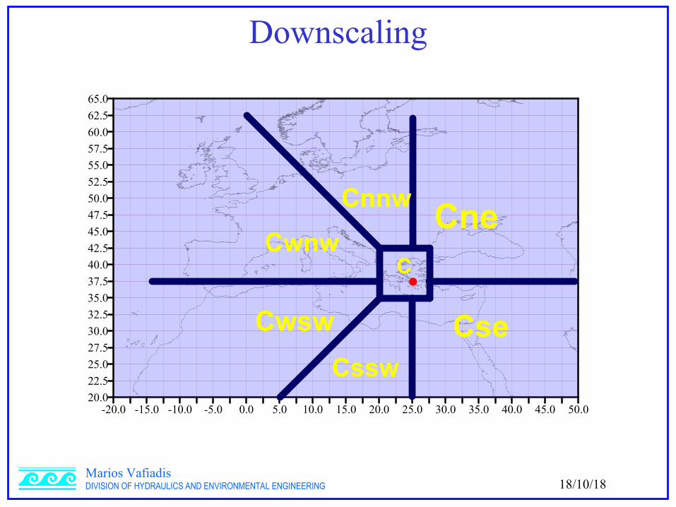
Downscaling
-20.0 -15.0 -10.0 -5.0 0.0 5.0 10.0 15.0 20.0 25.0 30.0 35.0 40.0 45.0 50.020.0
22.5
25.0
27.5
30.0
32.5
35.0
37.5
40.0
42.5
45.0
47.5
50.0
52.5
55.0
57.5
60.0
62.5
65.0
CneCnnw
Cwnw
Cwsw
Cssw
Cse
C

18/10/18Marios VafiadisDIVISION OF HYDRAULICS AND ENVIRONMENTAL ENGINEERING
Downscaling
-20.0 -15.0 -10.0 -5.0 0.0 5.0 10.0 15.0 20.0 25.0 30.0 35.0 40.0 45.0 50.020.0
22.5
25.0
27.5
30.0
32.5
35.0
37.5
40.0
42.5
45.0
47.5
50.0
52.5
55.0
57.5
60.0
62.5
65.0
AneAnw
Asw Ase
A

18/10/18Marios VafiadisDIVISION OF HYDRAULICS AND ENVIRONMENTAL ENGINEERING
Downscaling
Mean Annual Prec (mm) Mean numbers of raindays Pq95 (mm) Abs Max Prec (mm) Ratio AbsMax/Pq95
Athens 371.0 69 20.8 82.0 3.9GridAthens 330.8 105 14.9 111.2 7.5Thessaloniki 465.8 94 19.5 98.0 5.0GridThessaloniki 389.7 115 14.1 49.0 3.5Patra 660.9 83 25.6 86.6 3.4GridPatra 659.2 137 19.5 67.7 3.5Heraklio 507.1 72 27.4 222.2 8.1GridHeraklio 403.1 125 13.0 179.5 13.8

18/10/18Marios VafiadisDIVISION OF HYDRAULICS AND ENVIRONMENTAL ENGINEERING
Statistical downscaling model
• Predictor determination: 500hPa (NCEP and RCM data) spatial window (0oE – 32.5oE and 30oN – 55oN)
• Validation period: 15 years (1979-1993) common period for all the available data
• Predictants: seasonal precipitation heights for 6 stations in the Aravissos area and 2 stations in the Patra area
Artificial Neural Network approach
18/10/18Marios VafiadisDIVISION OF HYDRAULICS AND ENVIRONMENTAL ENGINEERING
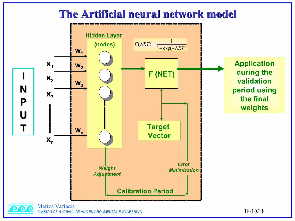
The Artificial neural network modelThe Artificial neural network model
IINNPPUUTT
Application during the validation
period using the final weights
x1
x2
x3
xn
Hidden Layer
(nodes)
F (NET)F (NET)
Target VectorTarget Vector
Error Minimization
Calibration Period
Weight Adjustment
ww11
ww22
ww33
wwnn
)exp(1
1)(
NETNETF

18/10/18Marios VafiadisDIVISION OF HYDRAULICS AND ENVIRONMENTAL ENGINEERING

18/10/18Marios VafiadisDIVISION OF HYDRAULICS AND ENVIRONMENTAL ENGINEERING
b. Dynamical downscaling model (RCM)
20 21 22 23 24 25 26 27 28
Spatial resolution of KNMI over Greece
35
36
37
38
39
40
41
20 21 22 23 24 25 26 27 28
35
36
37
38
39
40
41 Goumenissa
KariotisaK. Vrisi
Skydra
ExaplatanosTheodoraki
20 21 22 23 24 25 26 27 28
35
36
37
38
39
40
41
PatraAraksos

18/10/18Marios VafiadisDIVISION OF HYDRAULICS AND ENVIRONMENTAL ENGINEERING
c. Results for the validation period 1979-1993
0.0
50.0
100.0
150.0
200.0
250.0
300.0
mm
Araksos Patra
WINTER prec _ Validation period 1979-1993
Real ANNs KNMI
0.0
50.0
100.0
150.0
200.0
250.0
mm
ExaplatanosGoumenissa Kariotisa K.Vrisi Skydra Theodoraki
Winter prec _ Validation period 1979-1993
Real ANNs KNMIWinter Period
Aravissos
Patra
18/10/18Marios VafiadisDIVISION OF HYDRAULICS AND ENVIRONMENTAL ENGINEERING
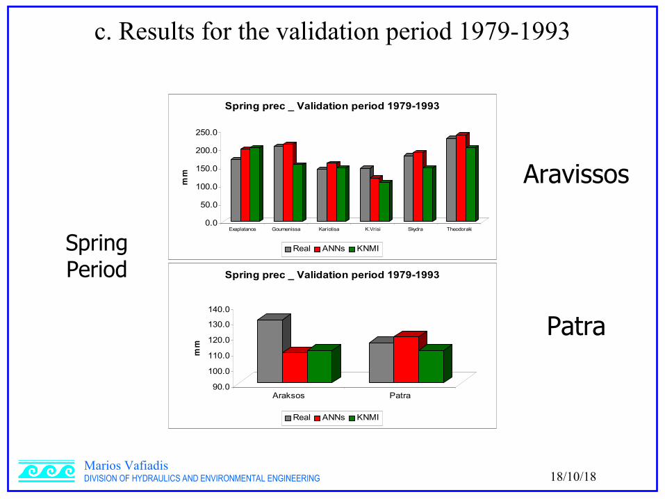
c. Results for the validation period 1979-1993
90.0
100.0
110.0
120.0
130.0
140.0
mm
Araksos Patra
Spring prec _ Validation period 1979-1993
Real ANNs KNMI
0.0
50.0
100.0
150.0
200.0
250.0
mm
Exaplatanos Goumenissa Kariotisa K.Vrisi Skydra Theodoraki
Spring prec _ Validation period 1979-1993
Real ANNs KNMISpring Period
Aravissos
Patra

18/10/18Marios VafiadisDIVISION OF HYDRAULICS AND ENVIRONMENTAL ENGINEERING
c. Results for the validation period 1979-1993
0.0
5.0
10.0
15.0
20.0
mm
Araksos Patra
Summer prec _ Validation period 1979-1993
Real ANNs KNMI
0.0
50.0
100.0
150.0
mm
Exaplatanos Goumenissa Kariotisa K.Vrisi Skydra Theodoraki
Summer prec _ Validation period 1979-1993
Real ANNs KNMISummer Period
Aravissos
Patra

18/10/18Marios VafiadisDIVISION OF HYDRAULICS AND ENVIRONMENTAL ENGINEERING
c. Results for the validation period 1979-1993
0.0
50.0
100.0
150.0
200.0
250.0
mm
Araksos Patra
Autumn prec _ Validation period 1979-1993
Real ANNs KNMI
0.0
50.0
100.0
150.0
200.0
250.0
300.0
mm
Exaplatanos Goumenissa Kariotisa K.Vrisi Skydra Theodoraki
Autumn prec _ Validation period 1979-1993
Real ANNs KNMIAutumn Period
Aravissos
Patra

18/10/18Marios VafiadisDIVISION OF HYDRAULICS AND ENVIRONMENTAL ENGINEERING
c. Results for the validation period 1979-1993
Araksos Patra Exaplatanos Goumenissa Kariotisa K.Vrisi Skydra TheodorakiANNs 0.7 0.6 -0.2 0.9 0.1 0.5 0.8 0.5KNMI 0.0 0.3 0.0 -0.3 0.0 -0.3 0.0 -0.1ANNs 0.4 0.4 0.2 0.2 -0.2 -0.4 0.3 0.2KNMI 0.4 0.3 0.2 0.6 0.0 0.3 0.2 0.4ANNs 0.2 0.0 0.6 0.7 0.7 0.3 0.7 0.8KNMI 0.0 0.1 0.3 0.2 0.2 0.3 0.4 0.3ANNs 0.0 0.1 0.3 0.4 0.1 0.5 0.5 0.2KNMI 0.0 -0.2 -0.1 0.1 -0.2 -0.1 -0.3 -0.2
AUTUMN
Real data
WINTER
SPRING
SUMMER
Correlation between the station and the simulated time – series for the validation
period
Scatter plot winter prec Goumenissa
0
100
200
300
400
500
0 100 200 300 400 500
Goumenissa Real
Go
um
enis
sa K
NM
IScatter plot winter prec Goumenissa
0
50
100
150
200
250
300
0 100 200 300 400 500
Goumenissa Real
Go
um
enis
sa A
NN
s

18/10/18Marios VafiadisDIVISION OF HYDRAULICS AND ENVIRONMENTAL ENGINEERING
Data and MethodologyStation rainfall data
For the Aravissos area seasonal data from six meteorological stations were available and used in the study:
- Goumenissa (1955-1995)- Exaplatanos (1975-2007)- Kariotisa (1969-2008)- Kria Vrisi (1951-1998)- Skydra (1959-1993)- Theodoraki (1975-2002)
For the Patra test sites the data from two stations were employed:
- Patra (1955 – 2005)- Araxos (1949-2007)

18/10/18Marios VafiadisDIVISION OF HYDRAULICS AND ENVIRONMENTAL ENGINEERING
Quality of estimation by comparison of estimated versus actual data
Season Statistical downscaling
RCM
Winter - +Spring + -
Summer OK -Autumn ~ -
Results 1. Results for the validation period

18/10/18Marios VafiadisDIVISION OF HYDRAULICS AND ENVIRONMENTAL ENGINEERING
2. Results for the control run period
Aravissos-test site.
Variable results depending of season and station.
Patra-test site.
Both models give smaller precipitation heights in respect to the observational ones.

18/10/18Marios VafiadisDIVISION OF HYDRAULICS AND ENVIRONMENTAL ENGINEERING
e. Future estimation for the seasonal precipitation (scenarios 2071-2100)
WinterAravissos-case study
0
50
100
150
200
250
300
350
400
1961
1963
1965
1967
1969
1971
1973
1975
1977
1979
1981
1983
1985
1987
1989
2022
2024
2026
2028
2030
2032
2034
2036
2038
2040
2042
2044
2046
2048
2050
2072
2074
2076
2078
2080
2082
2084
2086
2088
2090
2092
2094
2096
2098
2100
GRID1
meso-grid
Series3
171.6193.8
170.5
SpringAravissos-case study
0
50
100
150
200
250
300
350
1961
1963
1965
1967
1969
1971
1973
1975
1977
1979
1981
1983
1985
1987
1989
2022
2024
2026
2028
2030
2032
2034
2036
2038
2040
2042
2044
2046
2048
2050
2072
2074
2076
2078
2080
2082
2084
2086
2088
2090
2092
2094
2096
2098
2100
GRID1
meso-grid
Series3

18/10/18Marios VafiadisDIVISION OF HYDRAULICS AND ENVIRONMENTAL ENGINEERING
e. Future estimation for the seasonal precipitation (scenarios 2071-2100)
SpringAravissos-case study
0
50
100
150
200
250
300
350
1961
1963
1965
1967
1969
1971
1973
1975
1977
1979
1981
1983
1985
1987
1989
2022
2024
2026
2028
2030
2032
2034
2036
2038
2040
2042
2044
2046
2048
2050
2072
2074
2076
2078
2080
2082
2084
2086
2088
2090
2092
2094
2096
2098
2100
GRID1
meso-grid
Series3
143.2
161.3
105.1

18/10/18Marios VafiadisDIVISION OF HYDRAULICS AND ENVIRONMENTAL ENGINEERING
e. Future estimation for the seasonal precipitation (scenarios 2071-2100)
SummerAravissos-case study
0
20
40
60
80
100
120
1961
1963
1965
1967
1969
1971
1973
1975
1977
1979
1981
1983
1985
1987
198
9
2022
202
420
2620
28
2030
203
220
34
2036
203
820
4020
42
2044
2046
2048
205
0
2072
2074
207
620
7820
80
2082
2084
2086
2088
2090
2092
2094
2096
2098
2100
GRID1
meso-grid
Series3
16.2
24.3
13.9

18/10/18Marios VafiadisDIVISION OF HYDRAULICS AND ENVIRONMENTAL ENGINEERING
e. Future estimation for the seasonal precipitation (scenarios 2071-2100)
WinterPatra-case study
0
50
100
150
200
250
300
350
400
1961
1963
1965
1967
1969
1971
1973
1975
1977
1979
1981
1983
1985
1987
1989
2022
2024
2026
2028
2030
2032
2034
2036
2038
2040
2042
2044
2046
2048
2050
2072
2074
2076
2078
2080
2082
2084
2086
2088
2090
2092
2094
2096
2098
2100
gridpatra
Series3
223.3
SpringPatra-case study
0
50
100
150
200
250
1961
1963
1965
1967
1969
1971
1973
1975
1977
1979
1981
1983
1985
1987
1989
2022
2024
2026
2028
2030
2032
2034
2036
2038
2040
2042
2044
2046
2048
2050
2072
2074
2076
2078
2080
2082
2084
2086
2088
2090
2092
2094
2096
2098
2100
gridpatra
Series3
222.7
183.1

18/10/18Marios VafiadisDIVISION OF HYDRAULICS AND ENVIRONMENTAL ENGINEERING
e. Future estimation for the seasonal precipitation (scenarios 2071-2100)
SpringPatra-case study
0
50
100
150
200
250
1961
1963
1965
1967
1969
1971
1973
1975
1977
1979
1981
1983
1985
1987
1989
2022
2024
2026
2028
2030
2032
2034
2036
2038
2040
2042
2044
2046
2048
2050
2072
2074
2076
2078
2080
2082
2084
2086
2088
2090
2092
2094
2096
2098
2100
gridpatra
Series3
104.8121.0
85.6

18/10/18Marios VafiadisDIVISION OF HYDRAULICS AND ENVIRONMENTAL ENGINEERING
e. Future estimation for the seasonal precipitation (scenarios 2071-2100)
SummerPatra-case study
0
20
40
60
80
100
120
1961
1963
1965
1967
1969
1971
1973
1975
1977
1979
1981
1983
1985
1987
1989
2022
2024
2026
2028
2030
2032
2034
2036
2038
2040
2042
2044
2046
2048
2050
2072
2074
2076
2078
2080
2082
2084
2086
2088
2090
2092
2094
2096
2098
2100
meso-grid
Series3
3.7
6.7
4.4

18/10/18Marios VafiadisDIVISION OF HYDRAULICS AND ENVIRONMENTAL ENGINEERING
e. Future estimation for the seasonal precipitation (scenarios 2071-2100)
AutumnPatra-case study
0
50
100
150
200
250
300
350
400
45019
6119
6319
6519
6719
6919
7119
7319
7519
7719
79
1981
1983
198
519
8719
89
2022
2024
2026
2028
2030
2032
2034
2036
2038
2040
204
220
4420
46
204
820
50
2072
2074
2076
2078
2080
2082
2084
2086
2088
2090
2092
2094
2096
2098
210
0
gridpatra
Series3
143.4
138.7
136.6
Marios VafiadisDIVISION OF HYDRAULICS AND ENVIRONMENTAL ENGINEERING
And….That’s all for now!
Thank you for your attention!