shock-wave/boundary-layer interactions - nato educational...shock-wave/boundary-layer interactions 5...

RTO-EN-AVT-195 5 - 1

Shock-Wave/Boundary-Layer Interactions

Neil D. Sandham Aerodynamics and Flight Mechanics Research Group

University of Southampton Southampton SO17 1BJ

UK

[email protected]

ABSTRACT

In high speed intakes there are potentially far-reaching consequences of the interaction of shock waves with boundary layer since in extreme cases the interaction can cause an unstart of the intake. In this lecture we consider fundamental aspects of the interaction of shock waves with boundary layers, with an emphasis on understanding the origin of some of the physical phenomena that arise in simplified model problems. Cases with fully laminar, fully turbulent and transitional interactions are considered for the particular case of shock impingement on a flat plat. Unsteady effects are emphasised.

1.0 INTRODUCTION

In high Reynolds number flows the no-slip condition at solid surfaces leads to the formation of thin boundary layers in which the velocity and temperature adjust rapidly to meet the local free stream conditions. Seen from the point of view of a boundary layer, a shock wave is a localised pressure increase and is classified as an adverse pressure gradient. The effect of a moderate adverse pressure gradient is a thickening of the boundary layer, but in extreme cases the pressure gradient may be large enough to cause flow separation, which then has a global effect on the structure of the flow. In the context of an intake the region of flow separation may be confined to a small separation bubble, but can lead to a growing separation zone that will block the flow path and cause an unstart of the intake. A number of reviews [1,2,3] of shock-wave/boundary-layer interactions (SWBLI) are available in the published literature, but these predate a number of recent developments in experiments and numerical simulations. These notes are intended to provide an introduction to the physical phenomena that may occur when shock wave interact with boundary layers. Extensive use is made of recent results obtained using numerical simulations, which are providing much more detail on the flow physics than has been available from traditional experimental methods. At the same time laser-based techniques have advanced considerably in recent years and recent experimental work is also contributing to a much better understanding of SWBLI phenomena. It is hoped that these notes can be of use both as an introduction to the field and as a review of some of the recent advances for more experienced readers.

1.1 Model Problems In this contribution we shall be concerned with the fundamentals of SWBLI and will focus our attention on model problems that are simplified representations of the flowfields encountered in intakes. The most important simplification will be to flows that are two-dimensional in the mean i.e. homogeneous in the spanwise direction. It is important to recognise that, due to sidewall effects, typical wind tunnel experiments only approximate this condition (an exception is where the experiments are carried out for axisymmetric configurations), whereas it can be implemented exactly in numerical simulations. A number of potential candidate configurations are shown sketched in Figure 1. In Figure 1 (a) a shock wave is generated by a wedge placed in a supersonic free stream. The shock impinges and reflects from the boundary layer (the detailed flow structure near the reflected shock wave will be discussed later). In the


5 - 2 RTO-EN-AVT-195

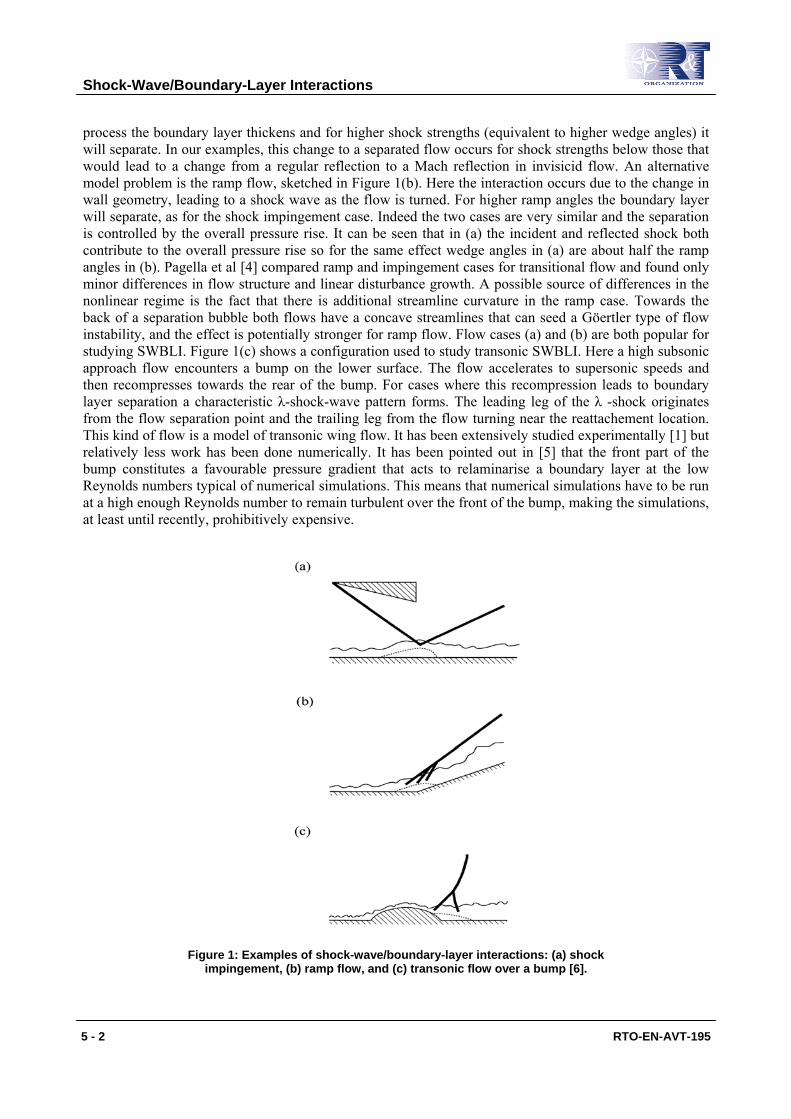
process the boundary layer thickens and for higher shock strengths (equivalent to higher wedge angles) it will separate. In our examples, this change to a separated flow occurs for shock strengths below those that would lead to a change from a regular reflection to a Mach reflection in invisicid flow. An alternative model problem is the ramp flow, sketched in Figure 1(b). Here the interaction occurs due to the change in wall geometry, leading to a shock wave as the flow is turned. For higher ramp angles the boundary layer will separate, as for the shock impingement case. Indeed the two cases are very similar and the separation is controlled by the overall pressure rise. It can be seen that in (a) the incident and reflected shock both contribute to the overall pressure rise so for the same effect wedge angles in (a) are about half the ramp angles in (b). Pagella et al [4] compared ramp and impingement cases for transitional flow and found only minor differences in flow structure and linear disturbance growth. A possible source of differences in the nonlinear regime is the fact that there is additional streamline curvature in the ramp case. Towards the back of a separation bubble both flows have a concave streamlines that can seed a Göertler type of flow instability, and the effect is potentially stronger for ramp flow. Flow cases (a) and (b) are both popular for studying SWBLI. Figure 1(c) shows a configuration used to study transonic SWBLI. Here a high subsonic approach flow encounters a bump on the lower surface. The flow accelerates to supersonic speeds and then recompresses towards the rear of the bump. For cases where this recompression leads to boundary layer separation a characteristic λ-shock-wave pattern forms. The leading leg of the λ -shock originates from the flow separation point and the trailing leg from the flow turning near the reattachement location. This kind of flow is a model of transonic wing flow. It has been extensively studied experimentally [1] but relatively less work has been done numerically. It has been pointed out in [5] that the front part of the bump constitutes a favourable pressure gradient that acts to relaminarise a boundary layer at the low Reynolds numbers typical of numerical simulations. This means that numerical simulations have to be run at a high enough Reynolds number to remain turbulent over the front of the bump, making the simulations, at least until recently, prohibitively expensive.

Figure 1: Examples of shock-wave/boundary-layer interactions: (a) shock impingement, (b) ramp flow, and (c) transonic flow over a bump [6].



1.2 Experimental Measurements The environment for SBLI is particularly challenging for experimental measurements, which until recently have been very restricted in terms of what could be measured with any degree of accuracy. Typical data available from older experiments consists of wall pressure, schlieren visualisation and some heat transfer and pitot probe data. Hot wire anemometer measurements in supersonic boundary layers are difficult and consequently are rarely available. The situation has changed very recently with the application of non-intrusive laser-based techniques to high speed flow. In particular particle-image-velocimetry (PIV) and laser-Doppler-anemometry (LDA) are now delivering much more complete measurements of the flow. Examples of recent studies using advanced diagnostics are available in [7,8], from which other literature in this area can be accessed.

1.3 Introduction to LES/DNS With increases in computer performance over the last ten years, large-eddy simulation (LES) and direct numerical simulation (DNS) have become feasible for transitional and turbulent SWBLI problems. In DNS an attempt is made to resolve all scales of the flow, but with the obvious limitation that the detailed structure of typical shocks cannot be resolved, but needs to be captured using special numerical methods. Nevertheless we class as DNS those simulations which resolve the flow down to the smallest viscous scale everywhere except in shock waves. The smallest scale is of the order of the Kolmogorov scale in free flow or of the order of a viscous wall unit ( /v uτ , where v is the kinematic viscosity and 2 /wuτ τ ρ= defines the friction velocity uτ in terms of the wall shear stress wτ ) in a turbulent boundary layer. We use the term LES for simulations in which the smallest viscous scales are modelled, either with an explicit sub-grid model in traditional LES or by numerical dissipation or filtering in some recent variants. Experience shows that LES can give excellent results so long as resolution is not too far away (factors of grid spacing within three or four in wall-parallel directions and a factor of two in a wall-normal direction) from that which would be necessary for DNS. Knowing what the resolution requirement is for a DNS is a challenge, only really resolvable by extensive grid refinement studies and detailed monitoring of spectra.

Numerical methods for flows with shock waves and turbulence is a separate subject (see for example the recent review [9]) that we won’t address here. The simulation results that are presented here were all carried out with a high-order finite difference code that was coupled with traditional shock-capturing methods but with careful attention to limiting the shock treatment to a region very close to the shock and avoiding the use of shock capturing in regions dominated by vorticity (i.e. boundary layers). The numerical methods are covered in [10, 11, 12].

1.4 Overview In this contribution we shall focus on the shock-impingement test case and make use of recent DNS and LES to illustrate some of the flow phenomena occurring in SWBLI. We first consider purely laminar interactions and then move to transitional interactions, taking into account cases where the transition starts from small amplitude disturbances and then cases where there is a strong interaction between turbulent spots and a shock-induced separation bubble. Finally we will consider turbulent interactions, exploiting results from recent combined experimental and numerical investigations [13]. A particular issue that principally occurs for turbulent interactions is a high-amplitude low-frequency broadband spectral peak seen for example in the wall pressure measured near the origin of a reflected shock wave. Recent work suggests that simplified modelling of the phenomenon is possible, based on insights obtained from LES.

2.0 LAMINAR INTERACTION Figure 2 (taken from [14]) illustrates the configuration for shock impingement studies and includes the flat plate from the experimental configuration and a computational domain for calculations. To avoid



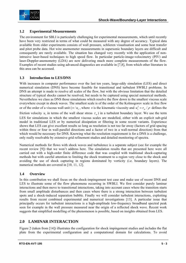
numerical issues associated with a leading edge, the computational box starts with a self-similar laminar boundary layer solution that would only be obtained in experiment some distance downstream of the leading edge. Computational co-ordinates are denoted with x, y while the global Rex is defined relative to the leading edge of the flat plate, assuming a self-similar development from there to the computational domain inflow. Within the computational domain, region (1) is the reference freestream, region (2) is after the impinging shock wave and region (3) is after the interaction. The total pressure rise over the interaction is p3/p1. The wedge generating the impinging shock does not need to be included in the calculation as the upper boundary condition can be written to include the correct shock-jump relations. In the configuration shown in Figure 2 the shock is strong enough to separate the boundary layer, leading to compression waves originating near the separation point and coalescing to form a shock further away from the wall. For strong interactions the shape of the separation bubble may be approximated by a triangle with the expansion fan forming over the apex at the top of the bubble and the other two corners at the separation and reattachment locations. In the reattachment region more compression waves are formed and further away from the surface these may merge with the compression waves originating at the separation point to form a single reflected shock. To avoid confusion later, we note that for turbulent interactions the boundary layer downstream is thicker and the recompression near the reattachment point is weaker, hence the reflected shock is generally taken to originate near the separation point.

Figure 2: Flow features of a laminar shock impingement configuration. The figure also shows the location of a typical computational domain and its relation to the

global Rex measured relative to the leading edge of the flat plate [14].

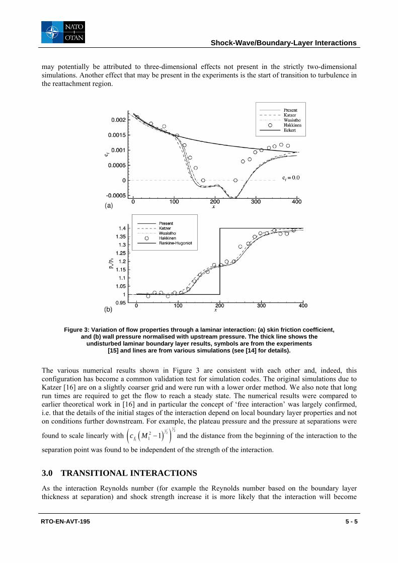
The model configuration of a nominally two-dimensional laminar interaction was first studied experimentally by Hakkinen et al.[15]. The symbols on Figure 3 show the experimental data compared to more recent work [14] that has solved the compressible Navier-Stokes equations numerically for the same configuration. The upstream Mach number is M=2.0 and the pressure ratio is p3/p1=1.4, corresponding to a 3.1˚ wedge angle. Figure 3(a) shows the skin friction and Figure 3(b) the wall pressure (normalised with the reference pressure p1). While the skin friction is difficult to measure experimentally, it can be seen that there is a good agreement in the wall pressure distribution. The main features are a rise in wall pressure starting near x=110, just before the boundary layer separation that occurs at x=140. The front half of the separation bubble is associated with a plateau in the pressure (becoming flatter as the strength of the interaction is increased). The skin friction shows that this part of the separation zone has moderately negative skin friction, while the rear part has strong recirculation and a more negative skin friction. The end of the pressure plateau corresponds quite closely with the location of minimum skin friction. In the example shown the reattachment occurs at x=280 and there is a slow recovery of pressure towards the pressure that one would get behind an inviscid shock reflection (shown in the sketch by the thick black line). Besides measurement error, the differences in the skin friction between experiment and simulation



may potentially be attributed to three-dimensional effects not present in the strictly two-dimensional simulations. Another effect that may be present in the experiments is the start of transition to turbulence in the reattachment region.

Figure 3: Variation of flow properties through a laminar interaction: (a) skin friction coefficient, and (b) wall pressure normalised with upstream pressure. The thick line shows the

undisturbed laminar boundary layer results, symbols are from the experiments [15] and lines are from various simulations (see [14] for details).

The various numerical results shown in Figure 3 are consistent with each other and, indeed, this configuration has become a common validation test for simulation codes. The original simulations due to Katzer [16] are on a slightly coarser grid and were run with a lower order method. We also note that long run times are required to get the flow to reach a steady state. The numerical results were compared to earlier theoretical work in [16] and in particular the concept of ‘free interaction’ was largely confirmed, i.e. that the details of the initial stages of the interaction depend on local boundary layer properties and not on conditions further downstream. For example, the plateau pressure and the pressure at separations were

found to scale linearly with ( )( )1

1 22

1

21 1fc M − and the distance from the beginning of the interaction to the

separation point was found to be independent of the strength of the interaction.

3.0 TRANSITIONAL INTERACTIONS

As the interaction Reynolds number (for example the Reynolds number based on the boundary layer thickness at separation) and shock strength increase it is more likely that the interaction will become



transitional. In this section we consider two scenarios, firstly where we have low amplitude disturbances in the boundary layer that can seed the growth of instabilities, and secondly where we are have high-amplitude free-stream disturbances that have already led to the formation of small turbulent spots, which then interact with the shock-induced separation bubble.

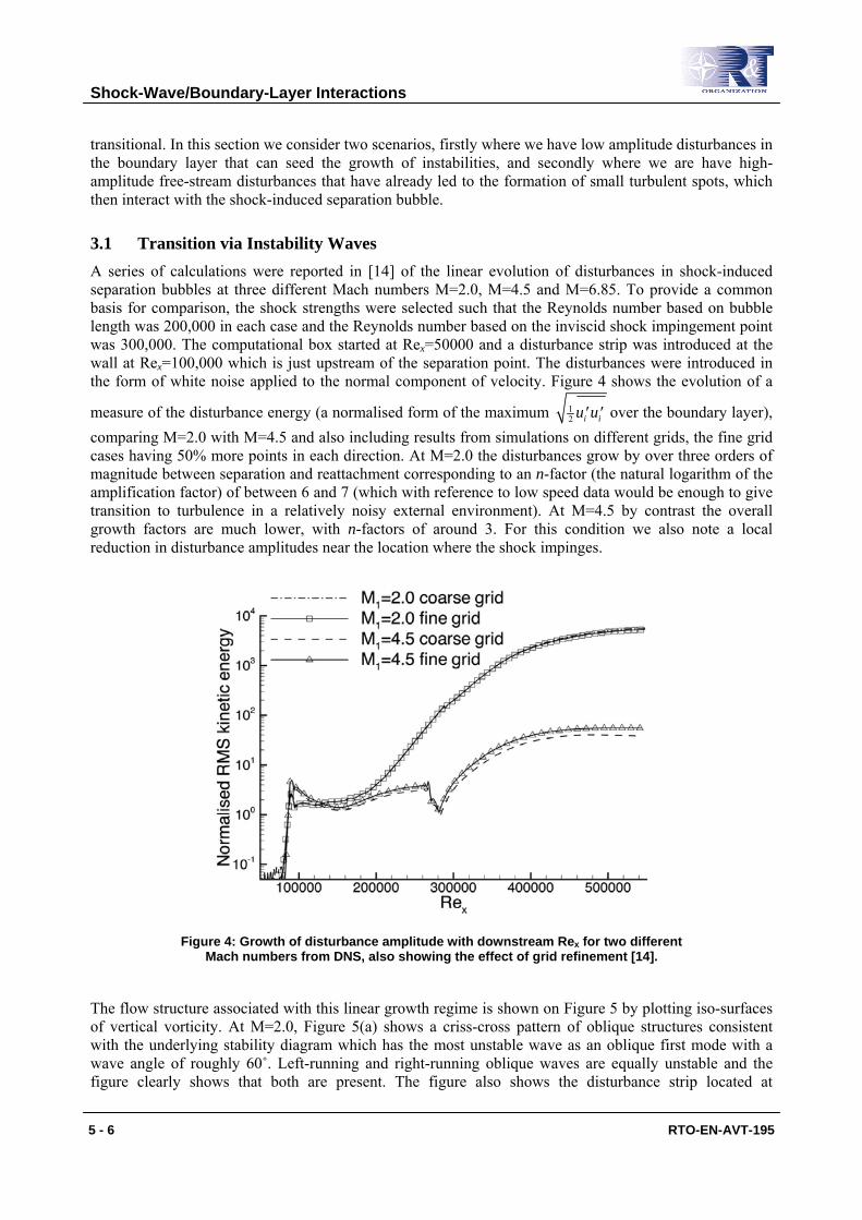
3.1 Transition via Instability Waves A series of calculations were reported in [14] of the linear evolution of disturbances in shock-induced separation bubbles at three different Mach numbers M=2.0, M=4.5 and M=6.85. To provide a common basis for comparison, the shock strengths were selected such that the Reynolds number based on bubble length was 200,000 in each case and the Reynolds number based on the inviscid shock impingement point was 300,000. The computational box started at Rex=50000 and a disturbance strip was introduced at the wall at Rex=100,000 which is just upstream of the separation point. The disturbances were introduced in the form of white noise applied to the normal component of velocity. Figure 4 shows the evolution of a

measure of the disturbance energy (a normalised form of the maximum 12 i iu u′ ′ over the boundary layer),

comparing M=2.0 with M=4.5 and also including results from simulations on different grids, the fine grid cases having 50% more points in each direction. At M=2.0 the disturbances grow by over three orders of magnitude between separation and reattachment corresponding to an n-factor (the natural logarithm of the amplification factor) of between 6 and 7 (which with reference to low speed data would be enough to give transition to turbulence in a relatively noisy external environment). At M=4.5 by contrast the overall growth factors are much lower, with n-factors of around 3. For this condition we also note a local reduction in disturbance amplitudes near the location where the shock impinges.

Figure 4: Growth of disturbance amplitude with downstream Rex for two different Mach numbers from DNS, also showing the effect of grid refinement [14].

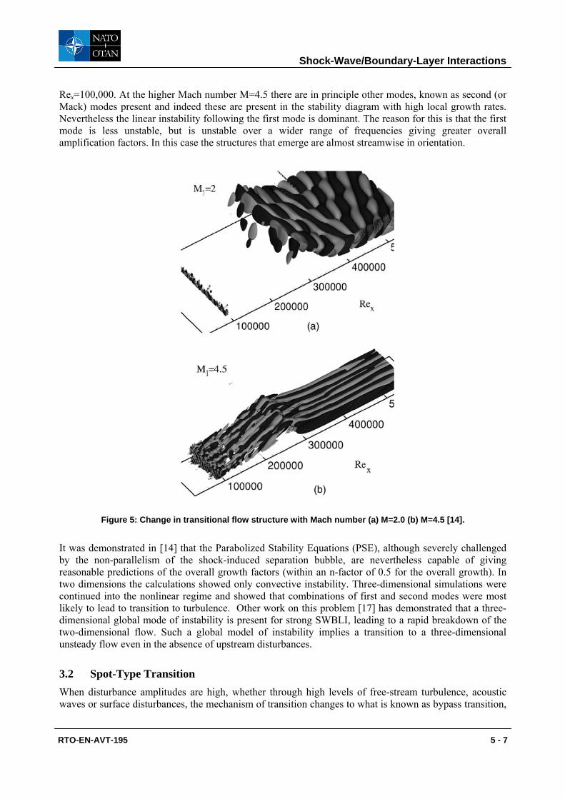
The flow structure associated with this linear growth regime is shown on Figure 5 by plotting iso-surfaces of vertical vorticity. At M=2.0, Figure 5(a) shows a criss-cross pattern of oblique structures consistent with the underlying stability diagram which has the most unstable wave as an oblique first mode with a wave angle of roughly 60˚. Left-running and right-running oblique waves are equally unstable and the figure clearly shows that both are present. The figure also shows the disturbance strip located at



Rex=100,000. At the higher Mach number M=4.5 there are in principle other modes, known as second (or Mack) modes present and indeed these are present in the stability diagram with high local growth rates. Nevertheless the linear instability following the first mode is dominant. The reason for this is that the first mode is less unstable, but is unstable over a wider range of frequencies giving greater overall amplification factors. In this case the structures that emerge are almost streamwise in orientation.

Figure 5: Change in transitional flow structure with Mach number (a) M=2.0 (b) M=4.5 [14].

It was demonstrated in [14] that the Parabolized Stability Equations (PSE), although severely challenged by the non-parallelism of the shock-induced separation bubble, are nevertheless capable of giving reasonable predictions of the overall growth factors (within an n-factor of 0.5 for the overall growth). In two dimensions the calculations showed only convective instability. Three-dimensional simulations were continued into the nonlinear regime and showed that combinations of first and second modes were most likely to lead to transition to turbulence. Other work on this problem [17] has demonstrated that a three-dimensional global mode of instability is present for strong SWBLI, leading to a rapid breakdown of the two-dimensional flow. Such a global model of instability implies a transition to a three-dimensional unsteady flow even in the absence of upstream disturbances.

3.2 Spot-Type Transition When disturbance amplitudes are high, whether through high levels of free-stream turbulence, acoustic waves or surface disturbances, the mechanism of transition changes to what is known as bypass transition,



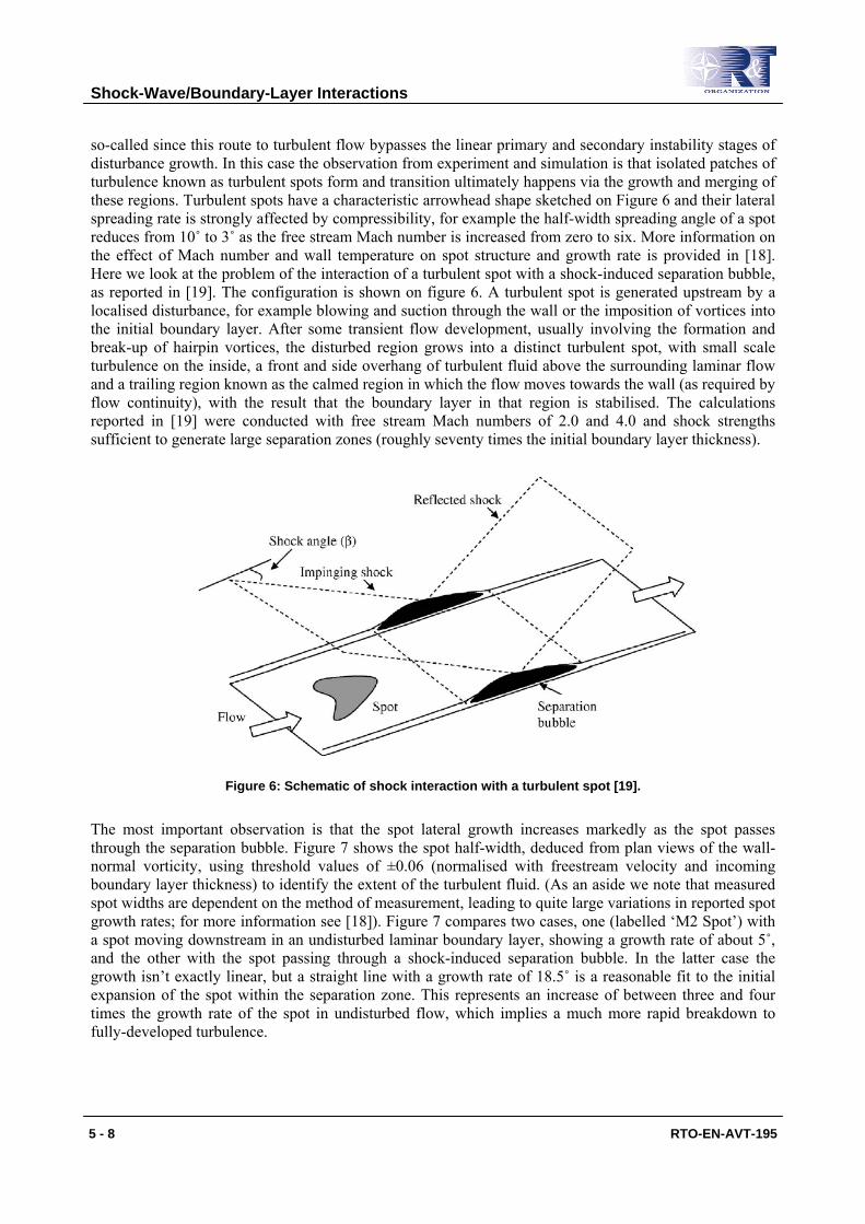
so-called since this route to turbulent flow bypasses the linear primary and secondary instability stages of disturbance growth. In this case the observation from experiment and simulation is that isolated patches of turbulence known as turbulent spots form and transition ultimately happens via the growth and merging of these regions. Turbulent spots have a characteristic arrowhead shape sketched on Figure 6 and their lateral spreading rate is strongly affected by compressibility, for example the half-width spreading angle of a spot reduces from 10˚ to 3˚ as the free stream Mach number is increased from zero to six. More information on the effect of Mach number and wall temperature on spot structure and growth rate is provided in [18]. Here we look at the problem of the interaction of a turbulent spot with a shock-induced separation bubble, as reported in [19]. The configuration is shown on figure 6. A turbulent spot is generated upstream by a localised disturbance, for example blowing and suction through the wall or the imposition of vortices into the initial boundary layer. After some transient flow development, usually involving the formation and break-up of hairpin vortices, the disturbed region grows into a distinct turbulent spot, with small scale turbulence on the inside, a front and side overhang of turbulent fluid above the surrounding laminar flow and a trailing region known as the calmed region in which the flow moves towards the wall (as required by flow continuity), with the result that the boundary layer in that region is stabilised. The calculations reported in [19] were conducted with free stream Mach numbers of 2.0 and 4.0 and shock strengths sufficient to generate large separation zones (roughly seventy times the initial boundary layer thickness).

Figure 6: Schematic of shock interaction with a turbulent spot [19].

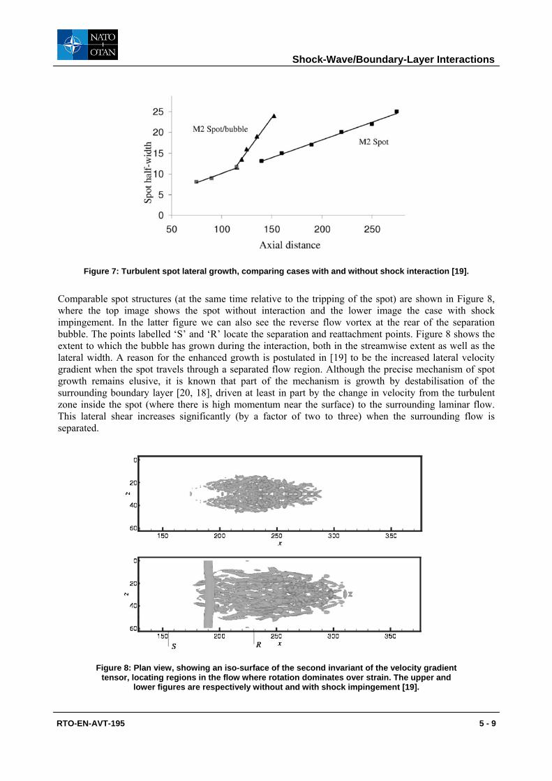
The most important observation is that the spot lateral growth increases markedly as the spot passes through the separation bubble. Figure 7 shows the spot half-width, deduced from plan views of the wall-normal vorticity, using threshold values of ±0.06 (normalised with freestream velocity and incoming boundary layer thickness) to identify the extent of the turbulent fluid. (As an aside we note that measured spot widths are dependent on the method of measurement, leading to quite large variations in reported spot growth rates; for more information see [18]). Figure 7 compares two cases, one (labelled ‘M2 Spot’) with a spot moving downstream in an undisturbed laminar boundary layer, showing a growth rate of about 5˚, and the other with the spot passing through a shock-induced separation bubble. In the latter case the growth isn’t exactly linear, but a straight line with a growth rate of 18.5˚ is a reasonable fit to the initial expansion of the spot within the separation zone. This represents an increase of between three and four times the growth rate of the spot in undisturbed flow, which implies a much more rapid breakdown to fully-developed turbulence.



Figure 7: Turbulent spot lateral growth, comparing cases with and without shock interaction [19].

Comparable spot structures (at the same time relative to the tripping of the spot) are shown in Figure 8, where the top image shows the spot without interaction and the lower image the case with shock impingement. In the latter figure we can also see the reverse flow vortex at the rear of the separation bubble. The points labelled ‘S’ and ‘R’ locate the separation and reattachment points. Figure 8 shows the extent to which the bubble has grown during the interaction, both in the streamwise extent as well as the lateral width. A reason for the enhanced growth is postulated in [19] to be the increased lateral velocity gradient when the spot travels through a separated flow region. Although the precise mechanism of spot growth remains elusive, it is known that part of the mechanism is growth by destabilisation of the surrounding boundary layer [20, 18], driven at least in part by the change in velocity from the turbulent zone inside the spot (where there is high momentum near the surface) to the surrounding laminar flow. This lateral shear increases significantly (by a factor of two to three) when the surrounding flow is separated.

Figure 8: Plan view, showing an iso-surface of the second invariant of the velocity gradient tensor, locating regions in the flow where rotation dominates over strain. The upper and

lower figures are respectively without and with shock impingement [19].


5 - 10 RTO-EN-AVT-195

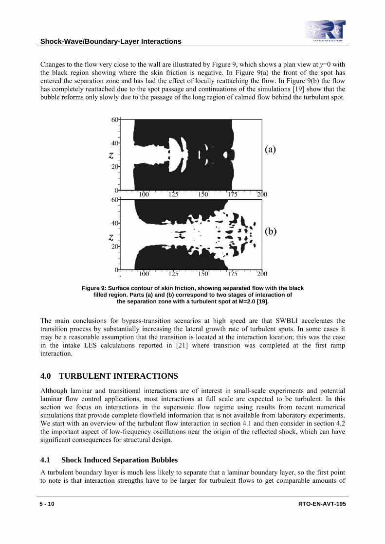
Changes to the flow very close to the wall are illustrated by Figure 9, which shows a plan view at y=0 with the black region showing where the skin friction is negative. In Figure 9(a) the front of the spot has entered the separation zone and has had the effect of locally reattaching the flow. In Figure 9(b) the flow has completely reattached due to the spot passage and continuations of the simulations [19] show that the bubble reforms only slowly due to the passage of the long region of calmed flow behind the turbulent spot.

Figure 9: Surface contour of skin friction, showing separated flow with the black filled region. Parts (a) and (b) correspond to two stages of interaction of

the separation zone with a turbulent spot at M=2.0 [19].

The main conclusions for bypass-transition scenarios at high speed are that SWBLI accelerates the transition process by substantially increasing the lateral growth rate of turbulent spots. In some cases it may be a reasonable assumption that the transition is located at the interaction location; this was the case in the intake LES calculations reported in [21] where transition was completed at the first ramp interaction.

4.0 TURBULENT INTERACTIONS

Although laminar and transitional interactions are of interest in small-scale experiments and potential laminar flow control applications, most interactions at full scale are expected to be turbulent. In this section we focus on interactions in the supersonic flow regime using results from recent numerical simulations that provide complete flowfield information that is not available from laboratory experiments. We start with an overview of the turbulent flow interaction in section 4.1 and then consider in section 4.2 the important aspect of low-frequency oscillations near the origin of the reflected shock, which can have significant consequences for structural design.

4.1 Shock Induced Separation Bubbles A turbulent boundary layer is much less likely to separate that a laminar boundary layer, so the first point to note is that interaction strengths have to be larger for turbulent flows to get comparable amounts of


RTO-EN-AVT-195 5 - 11

separated flow. The structure of a typical interaction is shown on Figure 10, taken from the work of Touber [22, 23]. Here the shock is generated by an 8˚ wedge in a flow at M=2.3 and impinged onto a flat plate turbulent boundary layer at Re=21,000 based on boundary layer displacement thickness at the impingement point in the absence of an interaction. The figure shows temperature contours from the LES and is labelled ‘IUSTI’ to denote the experimental flow conditions [24, 13] to which it was compared. The horizontal axis has been scaled so that the inviscid shock impingement is at x=0 and normalised with the boundary layer thickness at the impingement point, but in undisturbed flow. The wall is hot relative to the free stream and the boundary layer shows up as the blue zone, with white contours for the very highest temperatures. The impinging shock wave can be seen by the heating of the freestream fluid, starting from

4.5x = − on the upper boundary. The separation length is 2.9 in this scaling and the origin of the reflected shock is at 4x = − . The boundary layer is thickened by the interaction and recovers slowly downstream.

Figure 10: Visualisation of a turbulent SWBLI using temperature contours, from [22]. The horizontal axis has been shifted so that it is zero at the inviscid impingement point. The axes

are scaled with the boundary layer thickness at this point in the absence of an interaction.

Careful attention has to be paid in the simulation to the inflow boundary conditions used to trigger a rapid development of a turbulent boundary layer. Since one of the aims is to study low-frequency oscillations, it is important to monitor the frequency content of the inflow. In the simulations used as examples here a digital filter approach was used [22, 25] without any spikes in the spectrum. An alternative method based on synthetic disturbances [5] was also tested but not ultimately used due to the discrete frequencies that were introduced to trigger turbulence. Methods based on recycling were rejected due to the possibility of low-frequency content due to the recycling period, but we note that implementations of the recycling method using spanwise shifting are likely to remove this issue.

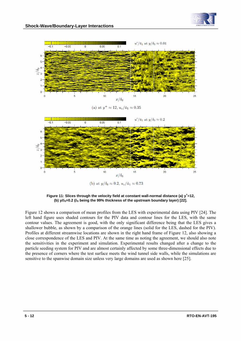
Figure 11 shows horizontal slices through the velocity field. In the very near-wall region in Figure 11(a) we can clearly see the formation of the streamwise velocity streaks that are a well-known characteristic of turbulent flow within and just outside the viscous sublayer. In wall units ( /y yuτ ν+ = ) the viscous sublayer is normally taken to extend to y+=8 and the streak amplitudes peak at roughly the y+=12 location shown in the figure. The separation and reattachment locations are shown with dashed white lines in the figure and it can be seen that the streaky pattern is completely disrupted by the separation bubble, with new streaks only forming well downstream of reattachment. Figure 11(b) shows the structure at

0.2y δ≈ i.e. at the outer edge of the overlap layer (but note in that a well-developed logarithmic region is not expected to form until much higher Reynolds numbers than are considered here). At this distance from the wall the velocity field is less coherent and the streamwise streaks that do form have a much lower aspect ratio compared to the near-wall structures. The separation zone has less of an impact at this location in the boundary layer, mainly causing an upward displacement of flow structures and an increase in the amplitude of the velocity fluctuations.


5 - 12 RTO-EN-AVT-195

Figure 11: Slices through the velocity field at constant wall-normal distance (a) y+=12, (b) y/δ0=0.2 (δ0 being the 99% thickness of the upstream boundary layer) [22].

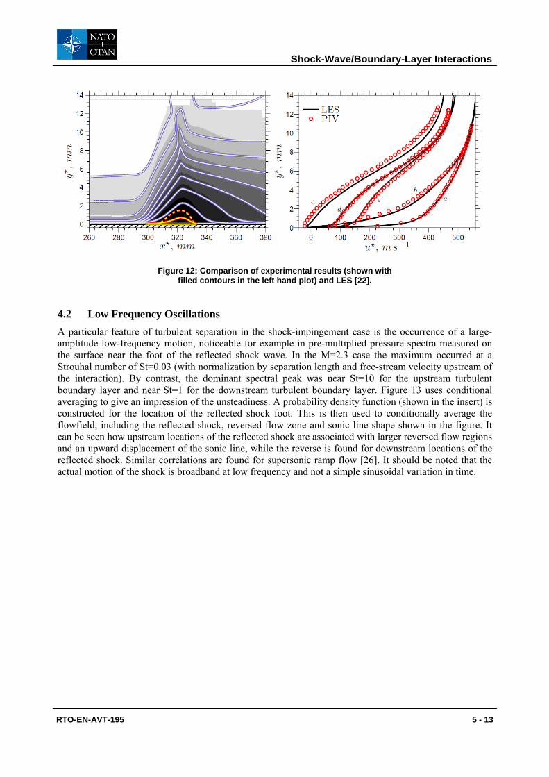
Figure 12 shows a comparison of mean profiles from the LES with experimental data using PIV [24]. The left hand figure uses shaded contours for the PIV data and contour lines for the LES, with the same contour values. The agreement is good, with the only significant difference being that the LES gives a shallower bubble, as shown by a comparison of the orange lines (solid for the LES, dashed for the PIV). Profiles at different streamwise locations are shown in the right hand frame of Figure 12, also showing a close correspondence of the LES and PIV. At the same time as noting the agreement, we should also note the sensitivities in the experiment and simulation. Experimental results changed after a change to the particle seeding system for PIV and are almost certainly affected by some three-dimensional effects due to the presence of corners where the test surface meets the wind tunnel side walls, while the simulations are sensitive to the spanwise domain size unless very large domains are used as shown here [25].


RTO-EN-AVT-195 5 - 13

Figure 12: Comparison of experimental results (shown with filled contours in the left hand plot) and LES [22].

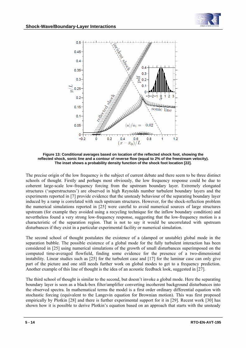
4.2 Low Frequency Oscillations A particular feature of turbulent separation in the shock-impingement case is the occurrence of a large-amplitude low-frequency motion, noticeable for example in pre-multiplied pressure spectra measured on the surface near the foot of the reflected shock wave. In the M=2.3 case the maximum occurred at a Strouhal number of St=0.03 (with normalization by separation length and free-stream velocity upstream of the interaction). By contrast, the dominant spectral peak was near St=10 for the upstream turbulent boundary layer and near St=1 for the downstream turbulent boundary layer. Figure 13 uses conditional averaging to give an impression of the unsteadiness. A probability density function (shown in the insert) is constructed for the location of the reflected shock foot. This is then used to conditionally average the flowfield, including the reflected shock, reversed flow zone and sonic line shape shown in the figure. It can be seen how upstream locations of the reflected shock are associated with larger reversed flow regions and an upward displacement of the sonic line, while the reverse is found for downstream locations of the reflected shock. Similar correlations are found for supersonic ramp flow [26]. It should be noted that the actual motion of the shock is broadband at low frequency and not a simple sinusoidal variation in time.


5 - 14 RTO-EN-AVT-195

Figure 13: Conditional averages based on location of the reflected shock foot, showing the reflected shock, sonic line and a contour of reverse flow (equal to 2% of the freestream velocity).

The inset shows a probability density function of the shock foot location [22].

The precise origin of the low frequency is the subject of current debate and there seem to be three distinct schools of thought. Firstly and perhaps most obviously, the low frequency response could be due to coherent large-scale low-frequency forcing from the upstream boundary layer. Extremely elongated structures (‘superstructures’) are observed in high Reynolds number turbulent boundary layers and the experiments reported in [7] provide evidence that the unsteady behaviour of the separating boundary layer induced by a ramp is correlated with such upstream structures. However, for the shock-reflection problem the numerical simulations reported in [25] were careful to avoid numerical sources of large structures upstream (for example they avoided using a recycling technique for the inflow boundary condition) and nevertheless found a very strong low-frequency response, suggesting that the low-frequency motion is a characteristic of the separation region. That is not to say it would be uncorrelated with upstream disturbances if they exist in a particular experimental facility or numerical simulation.

The second school of thought postulates the existence of a (damped or unstable) global mode in the separation bubble. The possible existence of a global mode for the fully turbulent interaction has been considered in [25] using numerical simulations of the growth of small disturbances superimposed on the computed time-averaged flowfield, finding some evidence for the presence of a two-dimensional instability. Linear studies such as [25] for the turbulent case and [17] for the laminar case can only give part of the picture and one still needs further work on global modes to get to a frequency prediction. Another example of this line of thought is the idea of an acoustic feedback look, suggested in [27].

The third school of thought is similar to the second, but doesn’t invoke a global mode. Here the separating boundary layer is seen as a black-box filter/amplifier converting incoherent background disturbances into the observed spectra. In mathematical terms the model is a first order ordinary differential equation with stochastic forcing (equivalent to the Langevin equation for Brownian motion). This was first proposed empirically by Plotkin [28] and there is further experimental support for it in [29]. Recent work [30] has shown how it is possible to derive Plotkin’s equation based on an approach that starts with the unsteady


RTO-EN-AVT-195 5 - 15

momentum integral equation, applied only to the region near the separation point. In the analysis [30] all steps were checked using large-eddy simulation, including an order-of-magnitude analysis of the problem, which showed at highest order an equation for the mean flow (relating skin friction to momentum and pressure thicknesses) and at next order an equation for fluctuations in the location of the reflected shock foot, forced by stochastic fluctuations in skin friction.

A closed quantitative model was also proposed in [30], whereby the response under the shock foot may be predicted using only properties of the upstream flow and the impinging shock wave. The model is conceptually different to the first school of thought, since it only requires very low amplitude background disturbances in the flow and these don’t need to be in the form of coherent structures. Figure 14 shows the results from the model compared to experiment and LES. The power spectral density is weighted by pre-multiplying by the frequency and with this representation the LES shows the appearance of two peaks, one at high frequency corresponding to the turbulence (Strouhal numbers of order 10 based on interaction length) and one at low frequency (peaking at St=0.03) corresponding to the additional low-frequency spectral content found at the shock foot. The experimental data only captures the second of these peaks due to the limited frequency response of the probe. It can be seen that the simple model, forced with white noise, captures the low-frequency response very well.

Figure 14: Weighted (premultiplied) power spectral density of wall pressure under the reflected shock foot, comparing LES, experiment and a simplified model [29].

Despite the success of this modeling work, we should note that there are only limited experimental data and only a few simulations for calibration of the model. Particular issues that have to be addressed in experiments are the three-dimensionality of the mean flow and the presence of upstream disturbances. In simulations there are strict requirements placed on boundary conditions and for good spectra extremely long run times are required (much longer than is routine to extract the time-averaged statistics, for example).


5 - 16 RTO-EN-AVT-195

5.0 CONCLUSIONS AND OUTLOOK

Recent progress on SWBLI has been made possible by advances in computer hardware, making direct and large-eddy simulations feasible for transitional and fully turbulent interactions, and by the extension of advanced experimental diagnostics such as PIV to the supersonic flow regime. Model problems, such as the shock impingement cases discussed here, can now be extensively studied to map the flow structure and explore the physical mechanisms. With the availability of complete data it is also realistic to develop and refine models and to think realistically about flow control. There are numerous opportunities also to extend the techniques beyond the simple interactions that we have considered. Very little work has been carried out on flows with multiple SWBLI, in which separation zones may be affected by other flow phenomena (control jets, cavities etc.) Also it is now feasible to simulate three-dimensional corner flows and hence move beyond the framework of spanwise periodicity that has been used in most simulations to date. In the context of practical intake configurations it is also becoming feasible to run LES that can be at comparable conditions to wind tunnel tests. Full-scale conditions will remain difficult to achieve, without significant reliance on wall models, but there is also the hope that these models can be improved for compressible flows featuring SWBLI with reference to the datasets that are now becoming available.

6.0 ACKNOWLEDGEMENTS

The author has benefited from interactions with numerous past and present colleagues at the University of Southampton. In particular the contributions of Drs Emile Touber, Yufeng Yao and L. Krishnan are gratefully acknowledged.

7.0 REFERENCES

[1] Delery J. & Marvin, J.G. (1986). Shock-wave boundary layer interactions. AGARD-AG-280.

[2] Dolling, D.S. (2001) Fifty years of shock-wave/boundary-layer interaction research: What next? AIAA Journal 39(8), 1517-1531.

[3] Adamson, T.C. & Messiter, A.F. (1980) Analysis of two-dimensional interactions between shock waves and boundary layers. Ann. Rev. Fluid Mech. 12, 103-138.

[4] Pagella, A., Babucke, A. & Rist, U. (2004) Two-dimensional numerical investigations of small-amplitude disturbances in a boundary layer at Ma=4.8: Compression corner versus impinging shock waves. Phys Fluids 16(7), 2272-2281.

[5] Sandham, N.D., Yao, Y.F. Lawal, A.A. (2003). Large-eddy simulation of transonic turbulent flow over a bump. Int. J. Heat and Fluid Flow 24, 584-595.

[6] Lawal, A.A. (2002) Direct numerical simulation of transonic shock/boundary-layer interactions. PhD thesis, University of Southampton.

[7] Ganpathisubramani, B., Clemens, N.T. & Dolling, D.S. (2007) Effects of upstream boundary layer on the unsteadiness of shock-induced separation. J. Fluid Mech. 585, 369-394.

[8] Souverein, L.J., van Oudheusden, B.W., Scarano, F. & Dupont, P. (2009) Application of a dual-plane particle image velocimetry (dual-PIV) technique for the unsteadiness characterisation of a shock wave turbulent boundary layer interaction. Meas. Sci. Technol. 20, 074003 (16 pp).

[9] Pirozzoli, S. (2011) Numerical methods for high-speed flows. Ann. Rev. Fluid Mech. 43, 163-194.


RTO-EN-AVT-195 5 - 17

[10] Yee, H.C., Sandham, N.D & Djomeri, M.J. (1999) Low-dissipative high-order shock-capturing methods using characteristic-based filters. J. Comp. Phys. 150, 199-238.

[11] Sandham, N.D., Yee, H.C. & Li, Q. (2002) Entropy splitting for high-order numerical simulation of compressible turbulence. J. Comp. Phys. 178, 307-322.

[12] Ducros, F. Ferrand, V., Nicoud, F., Weber, C., Darraq, D, Gacherieu, C & Poinsot, T. (1999) Large-eddy simulation of the shock turbulence interaction. J. Comp. Phys. 152(2), 517-549.

[13] Doerffer, P. Hirsch, C., Dussauge, J.-P., Babinsky, H. & Barakos, G.N. (Eds.) (2010) Unsteady effects of shock wave induced separation. Notes on Numerical Fluid Mechanics and Interdisciplinary Design Volume 144, Springer.

[14] Yao, Y., Krishnan, L. Sandham, N.D. & Roberts, G.T. (2007). The effect of Mach number on unstable disturbances in shock/boundary-layer interactions. Phys. Fluids 19, 054104.

[15] Hakkinen, R.J., Greber, I., Trilling, L. & Abarbanel, S.S. (1959). The interaction of an oblique shock wave with a laminar boundary layer. NASA MEMO 2-18-59W.

[16] Katzer, E. (1989) On the lengthscales of laminar shock/boundary-layer interaction. J. Fluid Mech. 206, 477-496.

[17] Robinet, J.-Ch. (2007) Bifurcations in shock-wave/boundary-layer interaction: global instability approach. J. Fluid Mech. 579, 85-112.

[18] Redford, J.A. , Sandham, N.D., & Roberts, G.T. (2011) Numerical simulations of turbulent spots in supersonic boundary layers: Effects of Mach number and wall temperature. Progress in Aerospace Sciences, in press, doi:10.1016/j.paerosci.2011.08.002.

[19] Krishnan, L. & Sandham, N.D. (2007) Strong interaction of a turbulent spot with a shock-induced separation bubble. Phys. Fluids 19, 016102.

[20] Gad-el-Haq, M., Blackwelder, R.F. & Riley, J.J. (1981) On the growth of turbulent regions in laminar boundary layers. J. Fluid Mech. 110, 73-96.

[21] Krishnan, L., Sandham, N.D. & Steelant, J. Shock-wave/boundary-layer interactions in a model scramjet intake. AIAA J. 47(7), 1680-1691.

[22] Touber, E. (2010) Unsteadiness in shock-wave/boundary-layer interactions. PhD thesis, University of Southampton.

[23] Touber, E & Sandham, N.D. (2009) Comparison of three large-eddy simulations of shock-induced turbulent separation bubbles. Shock Waves 19, 469-478.

[24] Dupont, P., Piponniau, S., Sidorenko, A. & Debiève, J.F. (2008) Investigation by particle image velocimetry measurements of oblique shock reflection with separation. AIAA J. 46(6), 1365-1370.

[25] Touber, E. & Sandham, N.D. (2009) Large-eddy simulation of low-frequency unsteadiness in a turbulent shock-induced separation bubble. Theor. Comput. Fluid Dyn. 23, 79-107.

[26] Wu, M. & Martin, M.P. (2008) Analysis of shock motion in shockwave and turbulent boundary layer interaction using direct numerical simulation data. J. Fluid Mech. 594, 71-83.


5 - 18 RTO-EN-AVT-195

[27] Pirozzoli, S. & Grasso, F. (2006) Direct numerical simulation of impinging shock wave/turbulent boundary layer interaction at M=2.25. Phys. Fluids 18, 065113.

[28] Plotkin, K.J. (1975) Shock wave oscillation driven by turbulent boundary layer fluctuations. AIAA J. 13(8), 1036-1040.

[29] Poggie, J. & Smits, A.J. (2005) Experimental evidence for Plotkin model of shock unsteadiness in separated flow. Phys. Fluids 17, 018107.

[30] Touber, E. & Sandham, N.D. (2011) Low-order stochastic modelling of low-frequency motions in reflected shock-wave/boundary-layer interactions. J. Fluid Mech. 671, 417-465.

shock-wave/boundary-layer interactions - nato educational...shock-wave/boundary-layer interactions 5...

Documents