ship-mounted real-time surface observational system on ... · pdf filedeployed on ships,...
TRANSCRIPT
Ship-Mounted Real-Time Surface Observational System on board Indian Vesselsfor Validation and Refinement of Model Forcing Fields*
R. HARIKUMAR AND T. M. BALAKRISHNAN NAIR
Indian National Centre for Ocean Information Services, Ministry of Earth Sciences, Government of India, Hyderabad, India
G. S. BHAT
Indian Institute of Science, Bengaluru, India
SHAILESH NAYAK
Earth System Science Organisation, New Delhi, India
VENKAT SHESU REDDEM AND S. S. C. SHENOI
Indian National Centre for Ocean Information Services, Ministry of Earth Sciences, Government of India, Hyderabad, India
(Manuscript received 16 November 2011, in final form 30 October 2012)
ABSTRACT
A network of ship-mounted real-time Automatic Weather Stations integrated with Indian geosynchronous
satellites [Indian National Satellites (INSATs)] 3A and 3C, named Indian National Centre for Ocean In-
formation Services Real-Time Automatic Weather Stations (I-RAWS), is established. The purpose of
I-RAWS is to measure the surface meteorological–ocean parameters and transmit the data in real time in
order to validate and refine the forcing parameters (obtained from different meteorological agencies) of the
Indian Ocean Forecasting System (INDOFOS). Preliminary validation and intercomparison of analyzed
products obtained from the National Centre for Medium Range Weather Forecasting and the European
Centre for Medium-Range Weather Forecasts using the data collected from I-RAWS were carried out. This
I-RAWS was mounted on board oceanographic research vessel Sagar Nidhi during a cruise across three
oceanic regimes, namely, the tropical IndianOcean, the extratropical IndianOcean, and the SouthernOcean.
The results obtained from such a validation and intercomparison, and its implicationswith special reference to
the usage of atmospheric model data for forcing ocean model, are discussed in detail. It is noticed that the
performance of analysis products from both atmospheric models is similar and good; however, European
Centre for Medium-RangeWeather Forecasts air temperature over the extratropical Indian Ocean and wind
speed in the Southern Ocean are marginally better.
1. Introduction
Indian National Centre for Ocean Information Ser-
vices (INCOIS) has established an ocean forecast system,
named the IndianOceanForecasting System (INDOFOS).
The purpose of this system is to predict ocean surface
waves, general circulation features, and oil spill trajec-
tories at various spatiotemporal scales. Forecast models
of this system are forced by the analyzed and forecasted
atmospheric products from the National Centre for
Medium Range Weather Forecasting (NCMRWF), the
European Centre for Medium-Range Weather Fore-
casts (ECMWF), the Global Forecast System (GFS),
and the Met Office. However, focused validation ex-
periments using independent in situ observations are
required to validate the forcing fields. An important
input to ocean models is the surface wind, which drives
the surface stress and fluxes of latent and sensible heat.
The wind field in the equatorial region is observed to be
inaccurate in the analysis and reanalysis data products
* Indian National Centre for Ocean Information Services Con-
tribution Number 125.
Corresponding author address: R. Harikumar, Indian National
Centre for Ocean Information Services, MoES, Government of
India, Hyderabad 500 090, India.
E-mail: [email protected]
626 JOURNAL OF ATMOSPHER IC AND OCEAN IC TECHNOLOGY VOLUME 30
DOI: 10.1175/JTECH-D-11-00212.1
� 2013 American Meteorological Society
(Ji and Smith 1995; Chen et al. 1999; Kelly et al. 1999;
Putman et al. 2000; PraveenKumar et al. 2013) and large
biases are present in heat fluxes (Bony et al. 1997; Smith
et al. 2001; Praveen Kumar et al. 2012). Errors in the
wind field are known to have an impact on the modeled
ocean circulation (Myers et al. 1998) and wave/swell
parameters (SWIM 1985).
Surface wind data are available from shallow- and
deep-water buoys at a few locations along the coasts of
India since 1999 (Harikumar et al. 2011). The India Me-
teorological Department (IMD) collects meteorological
data over oceans by an establishment of cooperation of
voluntary observing fleet (VOF) of ships (Attri and Tyagi
2010). VOF comprises merchant ships of Indian registry,
some foreign merchant vessels, and a few ships of the
Indian navy. These ships, while sailing on the high seas,
function as floating observatories. But the observations
are having sparse temporal resolution (only 6 hourly
at 0000, 0600, 1200, and 1800 UTC). Another drawback
is that the records of observations are passed on as
‘‘bulletins’’ to the IMD for analysis and archival, only
when the ships call at ports. International Compre-
hensive Ocean–Atmosphere Data Set (ICOADS) is a
project that has global weather observations taken near
the ocean’s surface since 1854, primarily from mer-
chant ships, into a compact and easy-to-use dataset of
28 3 28 spatial resolution (Woodruff et al. 1987). Re-
cently, the new release 2.5 of the ICOADS data range
from early noninstrumental ship observations to mea-
surements initiated in the twentieth century from buoys
and other automated platforms (Woodruff et al. 2010).
This newly released dataset has sparse spatial resolu-
tions of 28 3 28 (since 1800) and 18 3 18 (since 1960).
Gathering real-time in situ data over oceans for vali-
dation and assimilation is laborious and expensive if
cruises are exclusively dedicated for routine observa-
tions. Prior to 1970, ships were practically the only
source of observations, and now modern sensors are
deployed on ships, moored and drifting buoys, aircraft,
and Earth-observing satellites, providing a variety of
surface data (Smith 2011). The moored buoys ensure
data continuity, but their spatial coverage is limited as
they are few in number in the Indian Ocean region. The
availability of in situ measurements from the Indian
sector of the Southern Ocean is poor or nonexistent.
Merchant, passenger, and research vessels spend con-
siderable amount of time over the open ocean and can
make contributions to marine data collection, if auto-
mated ocean and atmosphere monitoring systems are
installed on board (Smith et al. 2001). Several coun-
tries, including India, have ongoing programs to collect
surface meteorological–ocean data from voluntary ob-
serving ships (VOSs, e.g., Hellerman and Rosenstien
1983; Da Silva et al. 1994; Servain et al. 1996; Bourassa
et al. 1997; Stricherz et al. 1996; Kent et al. 1998;
Unger 2005; Smith et al. 1999; Attri and Tyagi 2010).
But, most of them were designed to return data in
delayed modes.
To take advantage of the ships being operated by the
Indian agencies, INCOIS started INCOIS Real-Time
Automatic Weather Stations (I-RAWS) under the
Ocean Observations and Information Services (OOIS)
program of the Ministry of Earth Sciences (MoES),
government of India in the year 2009. Under this pro-
gram, automatic weather stations (AWSs) were installed
on board Indian research vessels with real-time data
transmission/reception by integration with Indian geo-
stationary satellites [Indian National Satellites (INSATs)]
3A and 3C. I-RAWS was installed on nine ships, and
there are plans to bring more ships under this program in
the coming years. I-RAWSmeasures air temperature, sea
surface temperature, air pressure, specific humidity, wind
speed and direction, rainfall, and downwelling short-
wave (SW) and longwave (LW) radiation. The data from
I-RAWS are also useful for the validation of satellite-
derived data products and for near-real-time assimilation
in forecast models. This will provide more initial condi-
tions for assimilation into models, which in turn will give
better forecasts. Real-time validation (displayed in real
time on the INCOIS website) of forecasted products
with I-RAWS data would enable users to judge them
better. Moreover, this program gives a large quantity of
surface meteorological–ocean data, especially in and
around the Indian coasts, while other existing VOS
datasets pertain mainly to the open ocean (Woodruff
et al. 2010; Attri and Tyagi 2010). These coastal data
would be valuable for assimilation and validation of
very high-resolution coastal models being planned by
INCOIS. Extensive validation exercises and real-time
data assimilation would definitely lead to better re-
finement of the forecasts.
A recent release by the National Oceanic and At-
mospheric Administration (NOAA) states, ‘‘For bud-
getary reasons, stemming from pending large cuts at the
NOAA Climate Program Office (CPO), ESRL [Earth
System Research Laboratory] Directors have de-
termined that it is no longer feasible for its Physical
Science Division (PSD) to continue supporting any
further ICOADS work—effective immediately. . . At
this juncture there are no plans for any new major
ICOADS delayed-mode updates or further Releases’’
(ICOADS 2012, p. 24). In this context, the establishment
of I-RAWS under the OOIS program of MoES, which
aims for data collection over the Indian Ocean, gains
importance and needs encouragement. The advantages
of I-RAWS are as follows. Important surface variables
MARCH 2013 HAR IKUMAR ET AL . 627
are measured along the ship track with a high temporal
resolution of 15 min; its data are available in real time
because of its integration with INSATs; it provides more
coastal data from ships, which are plying in and around
the Indian coasts and also from the data-sparse region,
namely, the Indian sector of the Southern Ocean; the
observation density in the Indian Ocean is expected
to increase because of the planned expansion of the
I-RAWS network, and I-RAWS data will be uploaded
to the Global Telecommunication System (GTS) soon
and hence the datasets will become publicly available.
One of the objectives of this paper is to bring the ex-
istence of the I-RAWS program to the notice of the
community. The other objective is to demonstrate how
useful the I-RAWS data are in validating the analyzed
products from NCMRWF and ECMWF (‘‘model
data’’), which are used to force the ocean forecast
models at INCOIS, using the data collected by I-RAWS
on board the oceanographic research vessel (ORV)
Sagar Nidhi during a cruise across three oceanic re-
gimes, that is, the tropical Indian Ocean (TIO; between
23.58N and 23.58S), the extratropical Indian Ocean
(ETIO; between 23.58 and 608S), and the Southern
Ocean (SO; south to 608S) during from 2 January to
24 April 2010. The configuration of the system is de-
scribed in section 2, followed by a description of the
datasets used for validation in section 3. Results are
shown in section 4, followed by a summary and conclu-
sions in section 5.
2. I-RAWS configuration
The basic variables measured by I-RAWS include air
temperature, sea surface temperature, pressure, relative
humidity (RH), downwelling solar and longwave radi-
ation, rainfall, wind speed, and wind direction. The
sensors selected for I-RAWS are similar to those used in
theResearchMooredArray forAfrican–Asian–Australian
Monsoon Analysis and Prediction (RAMA), the Tri-
angle Trans-Ocean Buoy Network (TRITON), and the
Prediction and Research Moored Array in the Tropical
Atlantic (PIRATA) mooring buoys under the Tropical
Atmosphere Ocean (TAO) project of the National
Oceanographic and Atmospheric Administration, United
States (Hayes et al. 1991; McPhaden et al. 2010). The
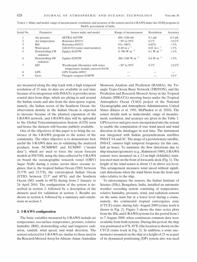
sensor details such as make/model, range of measure-
ment, resolution, and accuracy are given in the Table 1.
GPS receiver and gyro were incorporated into the system
to enable the computation of true wind speed and wind
direction in the datalogger in real time. The instrument
was integrated with Indian geosynchronous satellites
INSAT 3A and 3C. The usage of a geostationary satellite,
INSAT, ensures high temporal frequency (in this case,
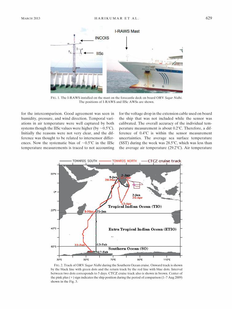
half an hour). To minimize the flow distortions due to
ship structure/geometry (e.g., Rahmstorf 1989), I-RAWS
sensors were mounted on a 2.5-m-high (foldable) stain-
less steel mast on the front of forecastle deck (Fig. 1). The
height of the wind sensor is about 13 m above sea level.
This arrangement measures wind speed without signifi-
cant distortions when the wind blows from the front and
sides relative to the ship.
To intercompare the sensors, the Indian Institute of
Science (IISc), Bengaluru, India, installed an automatic
weather recording system consisting of temperature,
relative humidity, pressure, wind, and radiation sensors
on the same mast but at a lower level during a cruise,
namely, the continental tropical convergence zone
(CTCZ) cruise, during July–August 2009 (cruise track is
shown in Fig. 2). Figure 3 shows the time series plots
from the IISc and I-RAWS systems for the period from 1
to 7 August 2009, when continuous common data were
available from both systems. During this period, the ship
was positioned at 88N, 858E (the location is shown on the
CTCZ cruise track in Fig. 2). In addition, a sonic ane-
mometer mounted on the ship at a height of 23 m as part
of its dynamical positioning (DP) system also was used
TABLE 1. Make and model, range of measurement, resolution, and accuracy of the sensors used in I-RAWS under the OOIS program of
MoES, government of India.
Serial No. Parameter Sensor make and model Range of measurement Resolution Accuracy
1 Air pressure SETRA-S1079W 800–1100 mb 0.1 mb 0.5 mb
2 Air temperature Rotronics-S93211 2508 to 508C 0.18C 60.28C3 RH Rotronics-S93211 0%–100% 0.02% ,3%
4 Wind speed Gill-S1510 (sonic wind monitor) 0–60 m s21 0.01 m s21 62%
5 Downwelling LW
radiation
Eppley-S1425W 0–700 W m22 0.1 W m22 61%
6 Downwelling SW
radiation
Eppley-S1092W 200–1200 W m22 0.4 W m22 62%
7 SST Weatherpak (thermistor with water
temperature module convert)-S3338
2508 to 508C 0.18C 60.28C
8 GPS GPS Trimble-S9922 — — —
9 Gyro Fluxgate compass-S1085W — — 60.18
628 JOURNAL OF ATMOSPHER IC AND OCEAN IC TECHNOLOGY VOLUME 30
for the intercomparison. Good agreement was seen in
humidity, pressure, and wind direction. Temporal vari-
ations in air temperature were well captured by both
systems though the IISc values were higher (by;0.58C).Initially the reasons were not very clear, and the dif-
ference was thought to be related to intersensor differ-
ences. Now the systematic bias of ;0.58C in the IISc
temperature measurements is traced to not accounting
for the voltage drop in the extension cable used on board
the ship that was not included while the sensor was
calibrated. The overall accuracy of the individual tem-
perature measurement is about 0.28C. Therefore, a dif-
ference of 0.48C is within the sensor measurement
uncertainties. The average sea surface temperature
(SST) during the week was 28.58C, which was less than
the average air temperature (29.28C). Air temperature
FIG. 1. The I-RAWS installed on the mast on the forecastle deck on board ORV Sagar Nidhi.
The positions of I-RAWS and IISc AWSs are shown.
FIG. 2. Track of ORV Sagar Nidhi during the SouthernOcean cruise. Onward track is shown
by the black line with green dots and the return track by the red line with blue dots. Interval
between two dots corresponds to 5 days. CTCZ cruise track also is shown in brown. Center of
the pink plus (1) sign indicates the ship position during the period of comparison (1–7Aug 2009)
shown in the Fig. 3.
MARCH 2013 HAR IKUMAR ET AL . 629
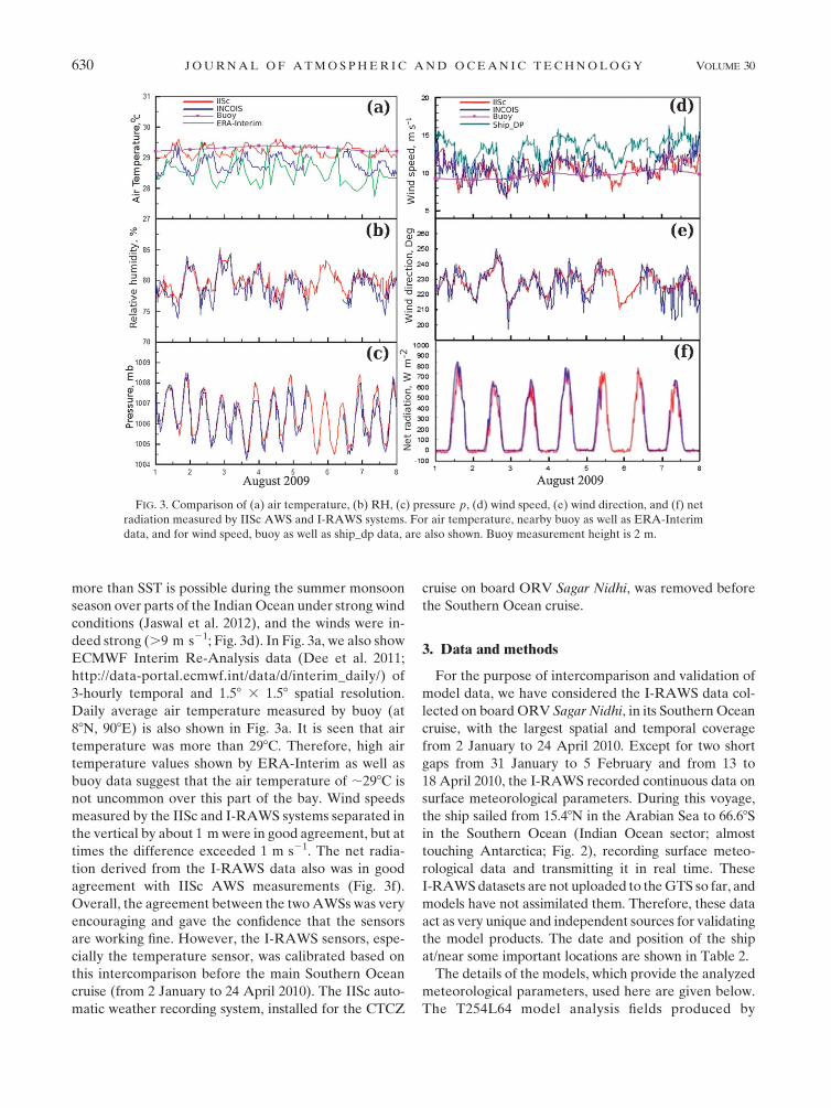
more than SST is possible during the summer monsoon
season over parts of the IndianOcean under strong wind
conditions (Jaswal et al. 2012), and the winds were in-
deed strong (.9 m s21; Fig. 3d). In Fig. 3a, we also show
ECMWF Interim Re-Analysis data (Dee et al. 2011;
http://data-portal.ecmwf.int/data/d/interim_daily/) of
3-hourly temporal and 1.58 3 1.58 spatial resolution.
Daily average air temperature measured by buoy (at
88N, 908E) is also shown in Fig. 3a. It is seen that air
temperature was more than 298C. Therefore, high air
temperature values shown by ERA-Interim as well as
buoy data suggest that the air temperature of ;298C is
not uncommon over this part of the bay. Wind speeds
measured by the IISc and I-RAWS systems separated in
the vertical by about 1 mwere in good agreement, but at
times the difference exceeded 1 m s21. The net radia-
tion derived from the I-RAWS data also was in good
agreement with IISc AWS measurements (Fig. 3f).
Overall, the agreement between the twoAWSs was very
encouraging and gave the confidence that the sensors
are working fine. However, the I-RAWS sensors, espe-
cially the temperature sensor, was calibrated based on
this intercomparison before the main Southern Ocean
cruise (from 2 January to 24 April 2010). The IISc auto-
matic weather recording system, installed for the CTCZ
cruise on board ORV Sagar Nidhi, was removed before
the Southern Ocean cruise.
3. Data and methods
For the purpose of intercomparison and validation of
model data, we have considered the I-RAWS data col-
lected on board ORV Sagar Nidhi, in its Southern Ocean
cruise, with the largest spatial and temporal coverage
from 2 January to 24 April 2010. Except for two short
gaps from 31 January to 5 February and from 13 to
18 April 2010, the I-RAWS recorded continuous data on
surface meteorological parameters. During this voyage,
the ship sailed from 15.48N in the Arabian Sea to 66.68Sin the Southern Ocean (Indian Ocean sector; almost
touching Antarctica; Fig. 2), recording surface meteo-
rological data and transmitting it in real time. These
I-RAWSdatasets are not uploaded to theGTS so far, and
models have not assimilated them. Therefore, these data
act as very unique and independent sources for validating
the model products. The date and position of the ship
at/near some important locations are shown in Table 2.
The details of the models, which provide the analyzed
meteorological parameters, used here are given below.
The T254L64 model analysis fields produced by
FIG. 3. Comparison of (a) air temperature, (b) RH, (c) pressure p, (d) wind speed, (e) wind direction, and (f) net
radiation measured by IISc AWS and I-RAWS systems. For air temperature, nearby buoy as well as ERA-Interim
data, and for wind speed, buoy as well as ship_dp data, are also shown. Buoy measurement height is 2 m.
630 JOURNAL OF ATMOSPHER IC AND OCEAN IC TECHNOLOGY VOLUME 30
NCMRWF at 6-hourly intervals were considered in this
study. This analysis utilizes all conventional and non-
conventional data received through the GTS at the re-
gional telecommunication hub (RTH) in New Delhi
(NCMRWF 2010). Nonconventional data include cloud
motion vectors (CMVs) from INSAT, the Japanese Geo-
stationary Meteorological Satellite (GMS), the Geosta-
tionary Operational Environmental Satellite (GOES),
and Meteorological Satellites (Meteosat); NOAA sat-
ellite temperature profiles and three-layer precipi-
table water content; surface wind information from the
European Remote Sensing Satellite-2 (ERS-2), etc.
(Parrish et al. 1997; Rizvi et al. 2000). ECMWF has in
the past produced three major reanalyses, namely, the
First Global Atmospheric Research Program Global
Experiment (FGGE), the 15-yr ECMWF Re-Analysis
(ERA-15; ECMWF 2008; Gibson and Uppala 1996),
and the 40-yr ECMWF Reanalysis (ERA-40; Uppala
et al. 2005). The last of these consisted of a set of global
analyses describing the state of the atmosphere and
land, and ocean wave conditions from mid-1957 to mid-
2002. ERA-Interim is an ‘‘interim’’ reanalysis of the
period 1989 to the present in preparation for the next-
generation extended reanalysis (Dee et al. 2011) to re-
place ERA-40. ERA-Interim was recently extended
backward by a decade to the year 1979, and it continues
to be updated forward in time. The ERA-Interim data
assimilation system uses a 2006 release of the Integrated
Forecast System (IFS Cy31r2), which contains many
improvements, both in the forecasting model and anal-
ysis methodology relative to ERA-40 (Dee et al. 2011).
The ERA-Interim reanalysis caught up with operations
in March 2009, and is now being continued in near–real
time to support climate monitoring. As part of the Year
of Tropical Convection (YOTC), ECMWFhas provided
the ERA-Interim analyzed fields for the year 2010 with
a spatial resolution of 0.1258 3 0.1258 online (at http://
data-portal.ecmwf.int/data/d/yotc_od/). The 12-h four-
dimensional variational data assimilation (4DVar)
scheme with in situ/satellite data assimilation is used in
the ERA-Interim reanalysis. ECMWF assimilates more
observation data than NCMRWF and gives more im-
portance for satellite observations than in situ observa-
tions (Simmons and Gibson 2000; Dee et al. 2011). The
spatial resolution of the YOTC data from ECMWF was
0.1258 3 0.1258, whereas that of the NCMRWF model
was 0.58 3 0.58. Hence, for the purpose of comparison,
the ECMWF data were regridded to a spatial resolution
of 0.58 3 0.58.The relative wind speed measured by the I-RAWS
was combined with the ship speed and direction pro-
vided byGPS and gyro to obtain the true wind speed and
direction. The models reported the wind speed at 10-m
height; hence, the true wind reported by I-RAWS was
logarithmically converted to 10-m height by using the
Monin–Obukhov similarity relations for the boundary
layer (Monin andObukhov 1954). NCMRWF reanalysis
provided specific humidity, and the corresponding hu-
midity variable was derived for ECMWF data using
dewpoint temperature and air pressure. Corresponding
I-RAWS specific humidity was calculated using mea-
sured relative humidity, air temperature, and air pres-
sure following Bolton (1980). I-RAWS data were 15-min
averages and essentially point measurements, while the
model data were 6-hourly averages over a 0.58 3 0.58area. Hence, for collocation purposes, the model data
corresponding to the grid(s) through which the ship
track passed through were extracted at a 6-hourly time
interval. I-RAWS data, averaged over the past 6 h, were
used while comparing the values at model output time
interval. In cases where the ship passed through more
than one model grid during the averaging period, the
area-weighted average of the model data was compared
with the I-RAWS data. Statistical parameters, namely,
bias, root-mean-square error (RMSE), and Pearson
correlation coefficient (r), were used to assess the agree-
ment between data.
4. Results and discussion
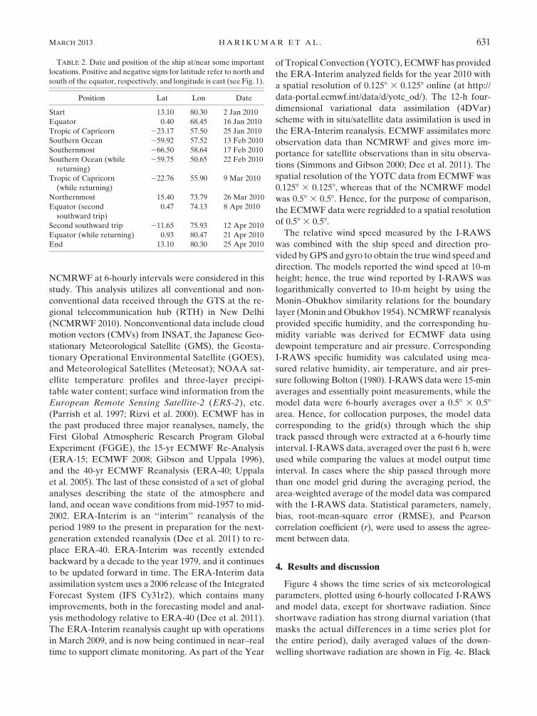
Figure 4 shows the time series of six meteorological
parameters, plotted using 6-hourly collocated I-RAWS
and model data, except for shortwave radiation. Since
shortwave radiation has strong diurnal variation (that
masks the actual differences in a time series plot for
the entire period), daily averaged values of the down-
welling shortwave radiation are shown in Fig. 4e. Black
TABLE 2. Date and position of the ship at/near some important
locations. Positive and negative signs for latitude refer to north and
south of the equator, respectively, and longitude is east (see Fig. 1).
Position Lat Lon Date
Start 13.10 80.30 2 Jan 2010
Equator 0.40 68.45 16 Jan 2010
Tropic of Capricorn 223.17 57.50 25 Jan 2010
Southern Ocean 259.92 57.52 13 Feb 2010
Southernmost 266.50 58.64 17 Feb 2010
Southern Ocean (while
returning)
259.75 50.65 22 Feb 2010
Tropic of Capricorn
(while returning)
222.76 55.90 9 Mar 2010
Northernmost 15.40 73.79 26 Mar 2010
Equator (second
southward trip)
0.47 74.13 8 Apr 2010
Second southward trip 211.65 75.93 12 Apr 2010
Equator (while returning) 0.93 80.47 21 Apr 2010
End 13.10 80.30 25 Apr 2010
MARCH 2013 HAR IKUMAR ET AL . 631
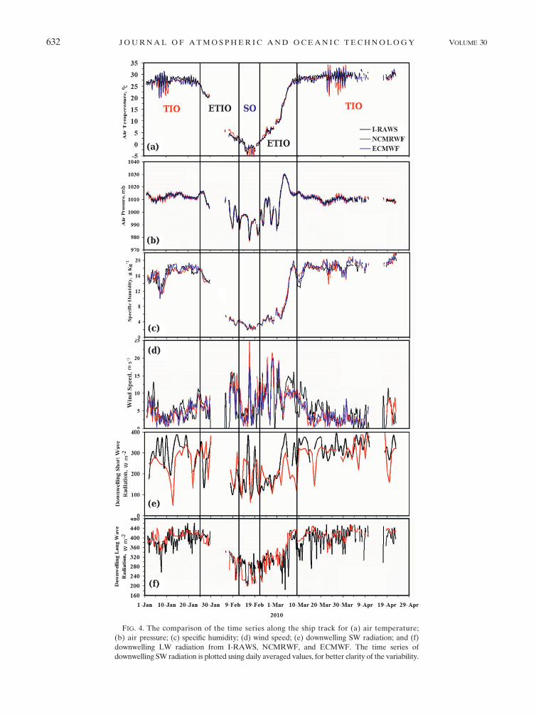
FIG. 4. The comparison of the time series along the ship track for (a) air temperature;
(b) air pressure; (c) specific humidity; (d) wind speed; (e) downwelling SW radiation; and (f)
downwelling LW radiation from I-RAWS, NCMRWF, and ECMWF. The time series of
downwelling SW radiation is plotted using daily averaged values, for better clarity of the variability.
632 JOURNAL OF ATMOSPHER IC AND OCEAN IC TECHNOLOGY VOLUME 30
vertical lines delineate different oceanic regimes.
Figure 5 shows the corresponding scatterplots of I-RAWS
observations against model data. The statistics are
summarized in Table 3. Two-tailed Student’s t test was
applied to assess the significance of all these statistical
parameters. It was found that all the statistical pa-
rameters are significant at the 95% confidence level.
This gives confidence in using the data from the SO,
though that was less in number compared to that from
the TIO and ETIO.
Figure 4 indicates that the latitudinal variations of all
variables were well captured by both models (exception
for longwave and shortwave radiation in NCMRWF
data). The model air temperature and surface pressure
show large amplitude (diurnal) variations in the TIO
and SO. This was true for both models. Examination of
the corresponding ship positions revealed that such ca-
ses were seen when the ship was moving along the coast
and at port calls, and the model grids contained both
land and sea areas. During the daytime, air temperature
was normally warmer over the land compared to that
over the ocean and vice versa during the nighttime.
Thus, while the model data reflected contributions from
land and sea, I-RAWS measured properties only over
water. The fact the model and I-RAWS diurnal varia-
tions differed in these cases is an indication that present-
day models are able to simulate mixed land–ocean grids
realistically. The best agreement in all variables was
seen in the ETIO (Fig. 5 and Table 3). For other ocean
basins also, the statistics improved when the values near
the coast were excluded. For example, in the TIO, the
correlation improved from 0.48 to 0.64 for air temper-
ature and that improved from 0.66 to 0.70 in case of
specific humidity when coastal data were excluded from
the analyses. In the case of wind speed, over the SO, the
correlation improved from 0.54 to 0.60 after the exclu-
sion of data near the coast. However, in the case of ra-
diation parameters, the scatter index increased when the
coastal data in the TIO and SO were excluded.
Goswami and Rajagopal (2003) had analyzed the
NCMRWF surface winds based on an earlier version of
model. They reported an easterly bias (1.0–1.5 m s21) in
the equatorial Indian Ocean (IO) and northerly bias
(2.0–3.0 m s21) in the south equatorial IO during 1999
and 2000 when compared with Quick Scatterometer
(QuikSCAT) winds. In the present case, the wind speed
bias is less than 1.0 m s21 between the in situ and
model data. This suggests that the new version of the
NCMRWF model used here has improved compared to
that existed during 1999–2000. The broad features of the
temporal variations in wind speed were captured well by
both models. RMSEs of NCMRWF and ECMWF were
comparable in the TIO (;2.7 m s21) and the ETIO
(;3.4 m s21); however, in the SO, the RMSE was less
for ECMWF (2.9 m s21) than that for NCMRWF
(4.6 m s21). Correlations in wind speed in the TIO and
ETIO for NCMRWF and ECMWF data are compara-
ble, but they are higher for ECMWF in the SO. Obvi-
ously, the ECMWF winds were better in the SO, where
the in situ observations are sparse.
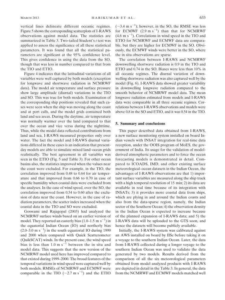
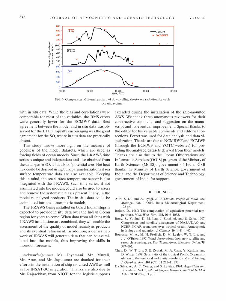
The correlation between I-RAWS and NCMRWF
downwelling shortwave radiation is 0.9 in the TIO and
ETIO and 0.74 in the SO. Biases were less than 10% in
all oceanic regimes. The diurnal variation of down-
welling shortwave radiation was also captured well by the
model (Fig. 6). I-RAWS data showed greater variability
in downwelling longwave radiation compared to the
smooth behavior of NCMRWF model data. The mean
longwave radiation estimated from models and I-RAWS
data were comparable in all three oceanic regimes. Cor-
relations between I-RAWS observations andmodels were
above 0.8 in the SO and ETIO, and it was 0.54 in the TIO.
5. Summary and conclusions
This paper described data obtained from I-RAWS,
a new surface monitoring system installed on board In-
dian vessels with INSAT integration for real-time data
reception, under the OOIS program of MoES, the gov-
ernment of India. Its usage for the validation of model-
derived atmospheric parameters and to force the ocean
forecasting models is demonstrated in detail. Com-
pared to ICOADS, IMD, and other existing surface
meteorological–ocean datasets in the Indian Ocean, the
advantages of I-RAWS observations are that 1) impor-
tant surface variables are measured along the ship track
with a high temporal resolution of 15 min; 2) its data are
available in real time because of its integration with
INSATs; 3) it provides more coastal data from ships,
which are plying in and around the Indian coasts and
also from the data-sparse region, namely, the Indian
sector of the Southern Ocean; 4) the observation density
in the Indian Ocean is expected to increase because
of the planned expansion of I-RAWS data; and 5) the
I-RAWS data will be uploaded to the GTS soon, and
hence the datasets will become publicly available.
Initially, the I-RAWS system was calibrated against
an AWS installed on board by IISc before taking it on
a voyage to the southern Indian Ocean. Later, the data
from I-RAWS collected during a longer voyage to the
southern Indian Ocean was used to validate the data
generated by two models. Results derived from the
comparison of all the six meteorological parameters
obtained from model analyzed products with I-RAWS
are depicted in detail in the Table 3. In general, the data
from the NCMRWF and ECMWFmodels matched well
MARCH 2013 HAR IKUMAR ET AL . 633
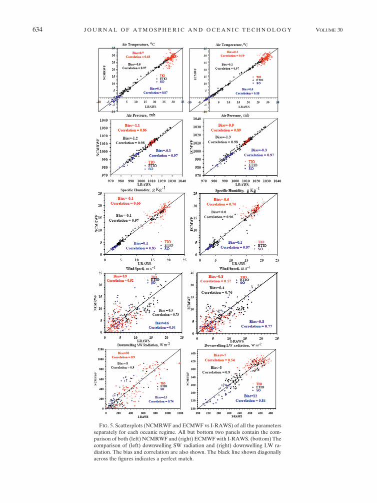
FIG. 5. Scatterplots (NCMRWF and ECMWF vs I-RAWS) of all the parameters
separately for each oceanic regime. All but bottom two panels contain the com-
parison of both (left) NCMRWF and (right) ECMWFwith I-RAWS. (bottom) The
comparison of (left) downwelling SW radiation and (right) downwelling LW ra-
diation. The bias and correlation are also shown. The black line shown diagonally
across the figures indicates a perfect match.
634 JOURNAL OF ATMOSPHER IC AND OCEAN IC TECHNOLOGY VOLUME 30
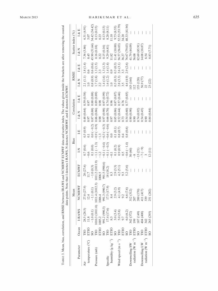
TABLE3.Mean,bias,correlation,andRMSEbetw
eenIR
AW
SandNCMRW
FECMW
Fdata
andscatterindex.Thevalues
giveninsidethebracketsare
afterremovingthecoastal
data
points.Note
thatIdenotesI-RAW
S,N
denotesNCMRWF,andEdenotesECMW
F.
Mean
Bias
Correlation
RMSE
Scatterindex(%
)
Parameter
Ocean
I-RAW
SNCMRW
FECMW
FI-N
I-E
I&
NI&
EI&
NI&
EI&
NI&
E
Air te
mperature
(8C)
TIO
28.5
(28.5)
27.8
(27.9)
28(27.6)
0.7
(0.6)
0.5
(0.9)
0.48(0.64)
0.59(0.58)
2.1
(1.1)
1.8
(1.4)
7.36(3.86)
6.31(4.91)
ETIO
11.8
12.4
11.7
20.6
0.1
0.97
0.97
1.0
0.6
8.45
5.07
SO
21.0
(0.1)
21.1
(0.1)
21.0
(0.3)
0.1
(0.0)
0.0
(20.2)
0.87(0.88)
0.88(0.88)
0.8
(0.9)
0.6
(0.6)
45.90(51.64)
34.42(34.42)
Pressure
(mb)
TIO
1010.3(1011.0)
1011.4(1012.3)
1011.2(1011.9)
21.1
(21.3)
20.9
(20.9)
0.86(0.86)
0.89(0.89)
1.7
(1.8)
1.3
(1.5)
0.16(0.18)
0.13(0.15)
ETIO
1005.2
1006.4
1006.5
21.2
21.3
0.98
0.98
2.2
2.3
0.22
0.23
SO
991.2
(990.3)
991.3
(990.7)
991.5
(990.6)
20.1
(20.4)
20.3
(20.3)
0.97(0.98)
0.97(0.99)
1.4
(1.6)
1.3
(1.3)
0.15(0.16)
0.13(0.13)
Specific
humidity(g
kg2
1)
TIO
17.4
(17.6)
17.5
(17.9)
18(18.2)
20.1
(20.3)
20.6
(20.6)
0.66(0.70)
0.74(0.72)
1.6
(1.2)
1.4
(1.4)
9.29(6.81)
8.20(8.11)
ETIO
8.3
8.4
8.3
20.1
0.0
0.97
0.96
1.0
0.9
11.82
11.10
SO
3.0
(3.4)
2.9
(3.2)
2.9
(3.3)
0.1
(0.2)
0.1
(0.1)
0.85(0.86)
0.87(0.87)
0.3
(0.3)
0.3
(0.3)
11.41(10.00)
9.73(8.53)
Windspeed(m
s21)
TIO
5.0
(5.8)
4.1
(4.9)
4.2
(5.1)
0.9
(0.9)
0.8
(0.7)
0.52(0.44)
0.57(0.46)
2.8
(3.3)
2.6
(3.1)
56.57(56.03)
52.53(53.79)
ETIO
9.7
9.2
9.3
0.5
0.4
0.73
0.76
3.5
3.3
36.27
34.20
SO
6.0
(6.2)
6.6
(7.6)
5.2
(5.6)
20.6
(21.4)
0.8
(0.6)
0.54(0.60)
0.77(0.85)
4.6
(4.9)
2.9
(2.6)
76.67(79.03)
48.33(41.94)
DownwellingSW
radiation(W
m22)
TIO
342(372)
312(312)
—30(60)
—0.90(0.90)
—143(164)
—41.79(44.09)
—
ETIO
199
207
—28
—0.90
—112
—56.08
—
SO
187(149)
200(170)
—213(21)
—0.74(0.92)
—155(128)
—82.69(85.91)
—
DownwellingLW
radiation(W
m22)
TIO
404(408)
411(417)
—27(2
9)
—0.54(0.45)
—56.9
(77)
—14.08(18.87)
—
ETIO
342
339
—3
—0.90
—22
—6.54
—
SO
263(293)
251(282)
—12(11)
—0.84(0.84)
—23(22)
—8.83(7.71)
—
MARCH 2013 HAR IKUMAR ET AL . 635
with in situ data. While the bias and correlations were
comparable for most of the variables, the RMS errors
were generally lower for the ECMWF data. Best
agreement between the model and in situ data was ob-
served for the ETIO. Equally encouraging was the good
agreement for the SO, where in situ data are practically
absent.
This study throws more light on the measure of
goodness of the model datasets, which are used as
forcing fields of ocean models. Since the I-RAWS time
series is unique and independent and also obtained from
the data-sparse SO, it has a lot of potential uses. Net heat
flux could be derived using bulk parameterizations if sea
surface temperature data are also available. Keeping
this in mind, the sea surface temperature sensor is also
integrated with the I-RAWS. Such time series, if not
assimilated into the models, could also be used to assess
and remove the systematic biases present, if any, in the
model reanalyzed products. The in situ data could be
assimilated into the atmospheric models.
The I-RAWS being installed on board Indian ships is
expected to provide in situ data over the Indian Ocean
region for years to come. When data from all ships with
I-RAWS installations are combined, they will enable the
assessment of the quality of model reanalysis products
and its eventual refinement. In addition, a denser net-
work of IRWAS will generate data that can be assimi-
lated into the models, thus improving the skills in
monsoon forecasts.
Acknowledgments. Mr. Jeyamani, Mr. Murali,
Mr. Arun, and Mr. Jayakumar are thanked for their
efforts in the installation of ship-mounted AWS as well
as for INSAT-3C integration. Thanks are also due to
Mr. Rajasekhar, from NIOT, for the logistic supports
extended during the installation of the ship-mounted
AWS. We thank three anonymous reviewers for their
constructive comments and suggestion on the manu-
script and its eventual improvement. Special thanks to
the editor for his valuable comments and editorial cor-
rections. Ferret was used for data analysis and data vi-
sualization. Thanks are due to NCMRWF and ECMWF
(through the ECMWF and YOTC websites) for pro-
viding the analyzed datasets derived from their models.
Thanks are also due to the Ocean Observations and
Information Services (OOIS) program of theMinistry of
Earth Sciences (MoES), government of India. GSB
thanks the Ministry of Earth Science, government of
India, and the Department of Science and Technology,
government of India, for support.
REFERENCES
Attri, S. D., and A. Tyagi, 2010: Climate Profile of India. Met
Monogr., No. 01/2010, India Meteorological Department,
122 pp.
Bolton, D., 1980: The computation of equivalent potential tem-
perature. Mon. Wea. Rev., 108, 1046–1053.
Bony, S., Y. Sud, K. M. Lau, J. Susskind, and S. Saha, 1997:
Comparison and satellite assessment of NASA/DAO and
NCEP–NCAR reanalyses over tropical ocean: Atmospheric
hydrology and radiation. J. Climate, 10, 1441–1462.
Bourassa, M. A., M. H. Freilich, D. M. Legler, W. T. Liu, and
J. J. O’Brien, 1997: Wind observations from new satellite and
research vessels agree.Eos, Trans. Amer. Geophys. Union, 78,
597–602.
Chen, D., W. T. Liu, S. E. Zebiak, M. A. Cane, Y. Kushnir, and
D. Witter, 1999: Sensitivity of the tropical Pacific Ocean sim-
ulation to the temporal and spatial resolution of wind forcing.
J. Geophys. Res., 104 (C5), 11 261–11 271.
Da Silva, A., A. C. Young, and S. Levitus, 1994: Algorithms and
Procedures.Vol. 1,Atlas of SurfaceMarine Data 1994,NOAA
Atlas NESDIS 6, 83 pp.
FIG. 6. Comparison of diurnal pattern of downwelling shortwave radiation for each
oceanic regime.
636 JOURNAL OF ATMOSPHER IC AND OCEAN IC TECHNOLOGY VOLUME 30
Dee, D. P., and Coauthors, 2011: The ERA-Interim reanalysis:
Configuration and performance of the data assimilation sys-
tem. Quart. J. Roy. Meteor. Soc., 137, 553–597, doi:10.1002/
qj.828.
ECMWF, 2008: Third WRCP International Conference on Re-
analysis. ECMWF Newsletter, No. 115, ECMWF, Reading,
United Kingdom, 3–5.
Gibson, R., and S. Uppala, 1996: The ECMWF Re-Analysis
(ERA) Project. ECMWF Newsletter, No. 73, ECMWF,
Reading, United Kingdom, 7–17.
Goswami, B. N., and E. N. Rajagopal, 2003: Indian Ocean surface
winds from NCMRWF analysis as compared to QuikSCAT
and moored buoy winds. J. Earth Syst. Sci., 112, 61–77.
Harikumar, R., L. Sabique, T. M. Balakrishnan Nair, and S. S. C.
Shenoi, 2011: Report on the assessment of wind energy po-
tential along the Indian coast for offshore wind farm advisories.
INCOIS Tech. Rep. INCOIS-MOG&ISG-TR-2011-07, 14 pp.
Hayes, S. P., L. J. Mangum, J. Picaut, A. Sumi, and K. Takeuchi,
1991: A moored array for real-time measurements in the
tropical Pacific Ocean. Bull. Amer. Meteor. Soc., 72, 339–347.
Hellerman, S., and M. Rosenstien, 1983: Normal monthly wind
stress over the World Ocean with error estimates. J. Phys.
Oceanogr., 13, 1093–1104.ICOADS, 2012: Transition meeting report: Monday 30 Jan. –Friday
3 Feb. 2012. NOAA/ESRL/PSD, 29 pp. [Available online at
http://icoads.noaa.gov/icoads-trans-rpt-v6-update.pdf.]
Jaswal, A. K., V. Singh, and S. R. Bhambak, 2012: Relationship
between sea surface temperature and surface air temperature
over Arabian Sea, Bay of Bengal and Indian Ocean. J. Indian
Geophys. Union, 16, 41–53.Ji, M., and T. M. Smith, 1995: Ocean model response to tempera-
ture data assimilation and varying surface wind stress: In-
tercomparisons and implications for climate forecast. Mon.
Wea. Rev., 123, 1811–1821.Kelly, K. A., S. Dickinson, and Z. J. Yu, 1999: NSCAT tropical
wind stress maps: Implications for improving ocean modeling.
J. Geophys. Res., 104 (C5), 11 291–11 310.
Kent, E. C., P. K. Taylor, and P. G. Challenor, 1998: A comparison
of ship- and scatterometer-derived wind speed data in open
ocean and coastal areas. Int. J. Remote Sens., 19, 3361–3381.
McPhaden,M. J., and Coauthors, 2010: The global tropical moored
buoy array. Proceedings of the OceanObs’09: Sustained Ocean
Observations and Information for Society, J.Hall,D.E.Harrison,
and D. Stammer, Eds., Vol. 2, ESA Publ. WPP-306.
Monin, A. S., and A. M. Obukhov, 1954: Basic laws of turbulent
mixing in the ground layer of the atmosphere. Tr. Geofiz. Inst.
Akad. Nauk. SSR, 151, 163–187.
Myers, P. G., K. Haines, and S. Josey, 1998: On the importance of
the choice of wind stress forcing to the modeling of the
Mediterranean Sea circulation. J. Geophys. Res., 103 (C8),
15 729–15 749.
NCMRWF, 2010: MONSOON-2009: Performance of the T254L64
Global Assimilation Forecast System. NCMRWF Monsoon
Rep. NMRF/MR/01/2010, 131 pp.
Parrish, D. F., J. Derber, J. Purser, W. Wu, and Z. Pu, 1997: The
NCEP Global Analysis System: Recent improvements and
future plans. J. Meteor. Soc. Japan, 75, 18 359–18 365.
Praveen Kumar, B., J. Vialard, M. Lengaigne, V. S. N. Murty, and
M. J. McPhaden, 2012: TropFlux: Air-sea fluxes for the global
tropical oceans—Description and evaluation. Climate Dyn.,
38, 1521–1543, doi:10.1007/s00382-011-1115-0.
——, ——, ——, ——, ——, M. F. Cronin, F. Pinsard, and
K. Gopala Reddy, 2013: TropFlux wind stresses over the
tropical oceans: Evaluation and comparison with other prod-
ucts. Climate Dyn., doi:10.1007/s00382-012-1455-4, in press.
Putman, W. M., D. M. Legler, and J. J. O’Brien, 2000: Interannual
variability of synthesized FSU and NCEP reanalysis pseudo-
stress products over the Pacific Ocean. J. Climate, 13, 3003–
3016.
Rahmstorf, F., 1989: Improving the accuracy of wind speed ob-
servations from ships. Deep-Sea Res., 36, 1267–1276.
Rizvi, S. R. H., R. Kamineni, and U. C. Mohanty, 2000: Report on
the assimilation of MSMR data in NCMRWF Global Data
Assimilation System. Department of Science and Technology,
NCMRWF, Scientific Rep. 1/2000, 72 pp.
Servain, J., J. N. Stricherz, and D. M. Legler, 1996: Tropical At-
lantic. Vol. 1, TOGA Pseudo-Stress Atlas 1985–1994. Centre
ORSTOM, 158 pp.
Simmons, A., and J. Gibson, 2000: The ERA project plan. ERA-40
Project Report Series No. 1, ECMWF Tech. Rep., 63 pp.
Smith, S. R., 2011: Ten-year vision for marine climate research.
Eos, Trans. Amer. Geophys. Union, 92, 376, doi:10.1029/
2011EO430005.
——, M. A. Bourassa, and R. J. Sharp, 1999: Establishing more
truth in true winds. J. Atmos. Oceanic Technol., 16, 939–952.
——, D. M. Legler, and K. V. Verzone, 2001: Quantifying un-
certainties in NCEP reanalyses using high-quality research
vessel observations. J. Climate, 14, 4062–4072.Stricherz, J. N., D. M. Legler, and J. J. O’Brien, 1996: Tropical
Pacific Ocean. Vol. 2, TOGA Pseudo-Stress Atlas 1985–1994,
COAPS Rep. 97–2, The Florida State University, 177 pp.
SWIM, 1985: Shallow water intercomparison of wave prediction
models (SWIM). Quart. J. Roy. Meteor. Soc., 111, 1087–
1113.
Unger, V., 2005: Presentation and evolution of the shipboard
automatic weather station BATOS. WMO Rep., 5 pp. [Avail-
able online at http://www.wmo.int/pages/prog/www/IMOP/
publications/IOM-82-TECO_2005/Papers/1(07)_France_Unger.
pdf.]
Uppala, S. M., and Coauthors, 2005: The ERA-40 Re-Analysis.
Quart. J. Roy. Meteor. Soc., 131, 2961–3012, doi:10.1256/
qj.04.176.
Woodruff, S. D., R. J. Slutz, R. L. Jenne, and P.M. Steurer, 1987: A
Comprehensive Ocean-Atmosphere Data Set. Bull. Amer.
Meteor. Soc., 68, 1239–1250.
——, and Coauthors, 2010: ICOADS release 2.5: Extensions and
enhancements to the surface marine meteorological archive.
Int. J. Climatol., 31, 951–967, doi:10.1002/joc.2103.
MARCH 2013 HAR IKUMAR ET AL . 637