shifts in portfolio preferences of international investors ... · banco de espaÑa 10 documento de...
TRANSCRIPT
SHIFTS IN PORTFOLIO PREFERENCES OF INTERNATIONAL INVESTORS: AN APPLICATION TO SOVEREIGN WEALTH FUNDS
Filipa Sá and Francesca Viani
Documentos de Trabajo N.º 1112
2011

SHIFTS IN PORTFOLIO PREFERENCES OF INTERNATIONAL INVESTORS:
AN APPLICATION TO SOVEREIGN WEALTH FUNDS
SHIFTS IN PORTFOLIO PREFERENCES OF INTERNATIONAL
INVESTORS: AN APPLICATION TO SOVEREIGN WEALTH FUNDS (*)
Filipa Sá (**)
UNIVERSITY OF CAMBRIDGE
Francesca Viani (***)
BANCO DE ESPAÑA
(*) The authors wish to thank Alan Sutherland, Anna Lipinska, an anonymous referee and seminar participants at the Bank of England, Bank of Spain, University of Cambridge and the 2009 INFINITI conference in Dublin for useful comments and suggestions.(**) Trinity College, University of Cambridge, [email protected].(***) Banco de España, [email protected].
Documentos de Trabajo. N.º 1112
2011

The Working Paper Series seeks to disseminate original research in economics and fi nance. All papers have been anonymously refereed. By publishing these papers, the Banco de España aims to contribute to economic analysis and, in particular, to knowledge of the Spanish economy and its international environment.
The opinions and analyses in the Working Paper Series are the responsibility of the authors and, therefore, do not necessarily coincide with those of the Banco de España or the Eurosystem.
The Banco de España disseminates its main reports and most of its publications via the INTERNET at the following website: http://www.bde.es.
Reproduction for educational and non-commercial purposes is permitted provided that the source is acknowledged.
© BANCO DE ESPAÑA, Madrid, 2011
ISSN: 0213-2710 (print)ISSN: 1579-8666 (on line)Depósito legal: M. 21858-2011Unidad de Publicaciones, Banco de España

Abstract
Reversals in capital infl ows can have severe economic consequences. This paper develops
a dynamic general equilibrium model to analyse the effect on interest rates, asset prices,
investment, consumption, output, the exchange rate and the current account of a shift in
portfolio preferences of foreign investors. The model has two countries and two asset classes
(equities and bonds). It is characterised by imperfect substitutability between assets and
allows for endogenous adjustment in interest rates and asset prices. Therefore, it accounts
for capital gains arising from equity price movements, in addition to valuation effects caused
by changes in the exchange rate. To illustrate the mechanics of the model, we calibrate it to
analyse the consequences of an increase in the importance of sovereign wealth funds (SWFs).
Specifi cally, we ask what would happen if ‘excess’ reserves held by emerging markets were
transferred from central banks to SWFs. We look separately at two diversifi cation paths: one
in which SWFs keep the same allocation across bonds and equities as central banks, but
move away from dollar assets (path 1); and another in which they choose the same currency
composition as central banks, but shift from US bonds to US equities (path 2). In path 1, the
dollar depreciates and US net debt falls on impact and increases in the long run. In path 2,
the dollar depreciates and US net debt increases in the long run. In both cases, there is a
reduction in the ‘exorbitant privilege’, ie, the excess return the United States receives on its
assets over what it pays on its liabilities. The model is applicable to other episodes in which
foreign investors change the composition of their portfolios.
Keywords: portfolio preferences, sudden stops, imperfect substitutability, global imbalances,
sovereign wealth funds.
JEL classifi cation: F32.

Resumen
Reversiones en los fl ujos de capital pueden comportar graves consecuencias económicas.
Este artículo desarrolla un modelo dinámico de equilibrio general para analizar el efecto
sobre tasas de interés, precios de los activos, inversión, consumo, producción, tipo de
cambio y cuenta corriente de un cambio en las preferencias de cartera de los inversores
extranjeros. El modelo consta de dos países y dos clases de activos (acciones y bonos). Se
caracteriza por sustituibilidad imperfecta entre los activos y permite ajustes endógenos de
tasas de interés y precios de los activos. Por lo tanto, incluye ganancias de capital debidas
a variaciones en el precio de las acciones, además de efectos de valoración debidos a
variaciones en el tipo de cambio. Para ilustrar la mecánica del modelo, lo calibramos para
analizar las consecuencias del crecimiento de los Fondos Soberanos de Inversión (FSI).
En concreto, nos preguntamos qué pasaría si el exceso de las reservas de los mercados
emergentes fuera transferido de los bancos centrales a los FSI. Nos fi jamos por separado
en dos estrategias de diversifi cación: una en la que los FSI mantienen el mismo reparto de
cartera entre bonos y acciones que los bancos centrales, pero se alejan de los activos en
dólares; otra en la que eligen la misma composición por monedas que los bancos centrales,
pero pasan de detener bonos de los EE.UU. a acciones de los EE.UU.. En el primer caso,
el dólar se depreciaría y la deuda neta de los EE.UU. caería en el corto plazo y aumentaría
en el largo plazo. En el segundo caso, el dólar se depreciaría y aumentaría la deuda neta
de los EE.UU. en el largo plazo. En ambos casos, habría una reducción en el «privilegio
exorbitante», el rendimiento en exceso que los EE.UU. reciben de sus activos respecto
a lo que pagan por sus pasivos. El modelo es aplicable a otros episodios en los que los
inversores extranjeros modifi can la composición de sus carteras.
Palabras claves: Preferencias de cartera, interrupciones en los fl ujos de capital, sustituibilidad
imperfecta, desequilibrios mundiales, fondos soberanos de inversión.
Códigos JEL: F32.

BANCO DE ESPAÑA 9 DOCUMENTO DE TRABAJO N.º 1112
1 Introduction
Reversals in capital inflows can have severe consequences for the real economy and the financial
sector, as the literature on sudden stops illustrates. This explains why global imbalances are seen
as one of the greatest vulnerabilities in the international monetary system. The sustainability of
global imbalances has been a major focus of the academic literature on international finance and is a
contentious topic. Some studies (for example, Blanchard, Giavazzi and Sá (2005) and Obstfeld and
Rogoff (2007)) find that global imbalances will not persist because the United States must stabilise
its external debt level, which would require a large depreciation of the dollar. Other studies find
that global imbalances can persist for a long period of time because of differences in financial market
development that make US assets attractive to foreign investors (for example, Caballero, Farhi and
Gourinchas (2008) and Forbes (2010)) or because of a persistent return differential between US and
foreign assets - the so-called ‘exorbitant privilege’ (Gourinchas and Rey (2007)).
The recent financial crisis exposed severe weaknesses in the US financial and regulatory system.
It would not have been surprising if investors had responded by reducing their holdings of US
assets. However, while foreign investors did sell US equities and corporate debt during the crisis,
their demand for US government debt increased sharply. This suggests that, even though the crisis
started in the United States, investors are still attracted by the safety and liquidity of US assets. Is
this situation likely to continue in the future? Or is foreign investors’ appetite for US assets likely
to diminish as US debt levels increase and tighter financial market regulations are adopted? What
would be the implications for the dollar exchange rate, global imbalances and asset prices of a shift
in the preferences of foreign investors away from US assets?
This paper develops a framework for understanding the implications for the dollar, interest rates,
asset markets and global imbalances of a shift in the portfolio preferences of foreign investors. It
develops a dynamic general equilibrium model with two regions (the United States and the rest
of the world (ROW)) and two goods (US and ROW-produced goods). A distinctive feature of
the model is the presence of two asset classes: equities and government bonds. This allows us to
study the implications of two types of changes in the portfolio preferences of foreign investors: a
reduction in their preference for US assets and a diversification away from US debt and into US
equity assets. The real exchange rate determines the allocation of goods and assets across the
two regions. Because each region issues both equities and bonds, there are four assets in total:
US equities, US government bonds, ROW equities, and ROW government bonds. These assets
are imperfect substitutes and their demand follows the specification in Blanchard, Giavazzi and
Sá (2005), where the share of wealth invested in each asset has an exogenous and an endogenous
component. The exogenous component represents shocks to portfolio preferences. The endogenous
component captures the reaction of asset demands to changes in the relative expected returns of
different assets.1
1A growing body of literature derives portfolio holdings from optimisation principles in stochastic general equi-librium settings. See, for instance, Devereux and Sutherland (2006) and Heathcote and Perri (2007). In this paper

BANCO DE ESPAÑA 10 DOCUMENTO DE TRABAJO N.º 1112
The general equilibrium nature of the model allows for endogenous adjustment in interest rates
and asset prices. Therefore, we can see how they are affected by shifts in the preferences of
foreign investors and what the implications are for the ‘exorbitant privilege’. Following any shock
to portfolio preferences, both equity and bond prices adjust to clear asset markets. Over time,
investors rebalance their portfolios in response to changes in expected returns. This endogeneity of
interest rates and asset prices is the key difference between our model and the one in Blanchard,
Giavazzi and Sá (2005), where interest rates are exogenous.
Our model is general enough to be usable for a variety of experiments. It could be calibrated
to countries outside the United States. For example, it could be used to study the implications
of the sudden reversals in capital flows that occurred in Iceland, Greece and Ireland during the
global financial crisis and to analyse the consequences for other countries with high debt levels if
foreign investors were to withdraw their investment. The model could also be used to understand
the implications of the ‘flight to safety’ observed during the crisis, with foreign investors moving
away from US equities and corporate debt into US government debt. To illustrate how the model
works, we use it to analyse the implications of an expansion in sovereign wealth funds (SWFs).
SWFs are government-owned investment funds, set up for a variety of purposes, for example to
transform the income from non-renewable natural resources into a diversified portfolio of assets or
to increase the return on foreign exchange reserves. SWFs are becoming increasingly important in
the international monetary system and are estimated to have between 2.1 and 3 trillion US dollars
of assets under management. While this is relatively small in comparison with total global financial
assets, estimated at $194 trillion in 2006 (IMF (2008b)), it is a sizable amount and exceeds the size
of hedge funds, estimated at $1.7 trillion. Moreover, SWFs are projected to grow rapidly in the
next decade and to have around $12 trillion of assets under management in 2015 (Morgan Stanley
(2007)).
Information about the portfolio structure of SWFs is relatively limited, since there is no uniform
public disclosure of their assets and investment strategies. Table 1 reports some available data on
the portfolio structure of SWFs. Information on currency composition is from the IMF COFER
data set and information on asset composition is from IMF (2008a). The portfolios of SWFs
are typically more diversified than traditional reserves held by central banks, with a larger share
invested in equities and a wider geographical dispersion. Given these differences in investment
strategies, a shift of reserve assets from central banks to SWFs could have implications for asset
prices, the flow of funds between countries, exchange rates, and the evolution of global imbalances.
In particular, SWFs may increasingly diversify away from dollar assets. This might lead to a
reduction in capital inflows into the United States, a depreciation of the dollar and an increase in
returns on dollar assets. SWFs may also diversify their portfolios away from low-risk, short-term
it is more convenient not to derive portfolio shares from microfoundations, but to adopt this ad hoc specification forasset demands. This allows us to match in the calibration international asset holdings with those observed in thedata abstracting from international risk-sharing issues. Moreover, in optimal portfolio choice models, the returns ondifferent assets coincide in a non-stochastic steady state. So, adopting that type of model would prevent us fromstudying the impact of shifts in preferences of foreign investors on the US exorbitant privilege.

BANCO DE ESPAÑA 11 DOCUMENTO DE TRABAJO N.º 1112
debt instruments, and into longer-term equity assets, which might lead to changes in asset prices
and rates of return.
The changes in asset returns generated by the growth in SWFs might induce a reduction in the
so-called ‘exorbitant privilege’ of the United States. This term has been used by Gourinchas and
Rey (2007) to denote the fact that the United States receives higher returns on its foreign assets
than it pays on its foreign liabilities. This excess return can be decomposed in two elements: a
return effect - within each asset class, the return that the United States pays to foreigners is smaller
than the return that foreigners pay to the United States; and a composition effect - the United
States tends to invest more in foreign equities, while foreigners tend to invest more in US bonds.
The growth in SWFs may lead to a reduction in both components of the ‘exorbitant privilege’.
We simulate a scenario where all ‘excess reserves’ currently held by central banks in emerging
market economies (EMEs) are transferred to SWFs, where ‘excess reserves’ are defined as being
above the level that would be required for liquidity purposes. We consider two diversification
paths: one in which SWFs keep the same asset allocation as central banks, ie, the same investment
shares in equities and bonds, but diversify away from dollar assets (path 1); and another in which
they keep the same currency composition, but shift towards a riskier portfolio in the US market,
with a larger share invested in US equities and a smaller share invested in US bonds (path 2).
We focus on the implications for the dollar exchange rate, the US trade deficit and net debt,
and the ‘exorbitant privilege’. We should highlight that the main purpose of our analysis is to
provide a qualitative assessment of how changes in portfolio preferences of foreign investors affect
asset returns, consumption, investment, the exchange rate, the trade deficit and net debt, and
to understand the channels through which these effects occur. Although the model is carefully
calibrated to match asset holdings and returns observed in the data, our analysis aims at providing
only a rough quantification of the magnitude of the adjustment in these variables.
Our results show that in path 1 (currency diversification) the dollar depreciates in the period
immediately after the shock, leading to a reduction in the US trade deficit and net debt. In sub-
sequent periods, the return on US assets must increase to clear asset markets. This generates a
rebalancing of the portfolios of foreign investors towards holding more dollar assets, which leads
to an appreciation of the dollar. The ‘exorbitant privilege’ in the United States, ie, the difference
between the return it receives on its foreign assets and the return it pays on its foreign liabilities,
decreases, and US net debt increases over time. In path 2 (asset diversification) the dollar de-
preciates and the US trade deficit decreases. However, US net debt increases over time due to a
reduction in the ‘exorbitant privilege’.
Qualitatively, our results can be compared with the findings of an exercise conducted by the IMF
(IMF (2008a)). It assumes that between 25% and 50% of new foreign currency inflows in countries
that have recently established SWFs will be invested by those SWFs. The exercise is calibrated
for two diversified portfolios: one which mimics the composition of Norway’s Government Pension
Fund; and another which is based on information on asset allocation and currency composition
provided in market analysis. These two stylised portfolios are compared with a scenario where

BANCO DE ESPAÑA 12 DOCUMENTO DE TRABAJO N.º 1112
assets are kept as central bank reserves. The results, derived using the IMF’s Global Integrated
Monetary Fiscal Model, suggest that the US real interest rate would increase by 10 to 20 basis
points, the dollar would depreciate by 2% to 5%, and the US current account deficit would improve
by 0.25 to 0.5 percentage points of GDP. In the rest of the world, real interest rates would fall,
currencies would appreciate, and domestic demand would increase. These results are qualitatively
similar to ours.
This paper is organised as follows. The structure of the model is explained in Section 2. Section
3 applies the model to study the implications of an expansion in SWFs. Section 4 concludes and
discusses avenues for future research.
2 The model
This section describes the simple general equilibrium model used for the simulations. The core
structure of the model is based on Ghosh (2007) and Meredith (2007). The model consists of
two regions: the United States and the rest of the world (ROW), each fully specialised in the
production of one homogeneous good. In each region, there are two types of assets: equities and
bonds. Equities are modelled as claims on the capital stock. Bonds are issued by the government,
who must balance its budget every period.
Each country is populated by a representative firm and two types of representative households:
entrepreneurs and portfolio investors. Firms in both regions produce output using capital and
labour, and adjust their productive capacity by increasing or decreasing their stock of capital. We
abstract from any nominal rigidity and from real economic growth. Entrepreneurs manage the
firms and have all their wealth invested in home equities. Portfolio investors invest in bonds and
equities at home and abroad. They supply labour inelastically and decide on the proportion of their
income to be allocated to consumption and portfolio investment. They receive income in the form
of wages and returns on their portfolio and pay taxes or receive transfers from the government.2
The general equilibrium nature of the model lets any adjustment in interest rates and asset
prices be determined endogenously, as asset demands react to changes in the relative expected
returns of different assets. The supply of equities is determined by firms’ investment in physical
capital. Because equity prices are determined endogenously, the model is able to account for capital
gains on equity holdings, in addition to valuation effects caused by changes in the exchange rate.
2We write the model with two types of households to ensure internal consistency. For the model to be internallyconsistent, firms should discount future profits using the discount factor of the consumers who manage them. Thesteady-state discount factor of portfolio investors is a function of the returns on all assets in which they invest (homeand foreign equities and bonds). However, the discount factor of US firms should equal, in steady state, the usercost of capital, which coincides with the rate of return on US equities. If there were only portfolio investors in theeconomy, for the discount factor of US portfolio consumers to equal the discount factor of US firms, the steady-statereturns on all four assets (home and foreign equities and bonds) would have to be the same. This would be anunattractive feature since we are interested in matching the return differential on assets observed in the data. Wesolve this problem by including two types of representative households: portfolio investors, who invest in all assets,and entrepreneurs, who only invest in home equities and manage the firms. The model is internally consistent sincethe discount factor of entrepreneurs equals the discount factor of the firms.

BANCO DE ESPAÑA 13 DOCUMENTO DE TRABAJO N.º 1112
2.1 Consumers
The size of the world population is normalised to 1, with a fraction n in the United States and
(1−n) in the rest of the world. There are two types of representative households in each economy:entrepreneurs and portfolio investors. Entrepreneurs manage the firms and invest all their wealth
in home equities. Portfolio investors supply labour inelastically, pay lump-sum taxes (or receive
transfers), and invest their wealth in both equities and bonds, at home and abroad. We denote
the fraction of entrepreneurs in the US population by αE and the fraction of entrepreneurs in the
ROW population by αE∗.Both entrepreneurs and portfolio investors decide on how much to consume given their wealth.
US households derive utility from consuming the following CES bundle of US and ROW-produced
goods:
Ct = (ρ)1/θ (CUS,t)θ−1θ + (1− ρ)1/θ (CROW,t)
θ−1θ
θθ−1
(1)
where ρ > 0.5 is a parameter capturing the degree of home bias in consumption and θ is the
elasticity of substitution between goods produced in different regions. Consumption in the ROW
is analogously defined, with starred variables denoting the corresponding quantities consumed by
ROW households.
The consumer price indices can be derived from the households’ cost minimisation problem.
Taking the home good as the numeraire, the consumer price index for the US is given by:
Pt = ρ+ (1− ρ) eθ−1t
11−θ
(2)
where et is the real exchange rate between the United States and ROW, defined as the relative
price of the goods produced in the two regions, so that an increase in the exchange rate represents
an appreciation of the dollar.
The demands of US consumers for domestically and foreign-produced goods are obtained from
standard cost minimisation subject to 1:
CUS,t = ρ (Pt)θ Ct (3)
CROW,t = (1− ρ) (etPt)θ Ct (4)
An appreciation of the dollar makes ROW goods less expensive to US consumers and US goods
more expensive to ROW households, shifting world demand from US to ROW-produced goods. In
this sense, the real exchange rate determines the allocation of goods across markets.
Consumers optimally decide to allocate their income between consumption and savings. The
utility maximisation problem for entrepreneurs is given by:

BANCO DE ESPAÑA 14 DOCUMENTO DE TRABAJO N.º 1112
max{CEs }∞s=t
. : Et
∞
s=t
Φs−t log CEt
s.t. : V Et = rEt VEt−1 − PtCEt
where V E represents the financial wealth of US entrepreneurs, rEt is the rate of return on their
portfolio defined in local currency and Φ is the discount factor. Because entrepreneurs invest all
their wealth in home equities, the rate of return on their portfolio equals the return on home
equities.
The utility maximisation problem for portfolio holders is given by:
max{CPs }∞s=t
. : Et
∞
s=t
Φs−t log CPt
s.t. : V Pt = RPt VPt−1 − PtCPt + wt − τ t
The key difference relative to the problem of entrepreneurs is in the budget constraint, which
now includes wage earning wt net of lump-sum taxes τ t. RPt is the rate of return on the portfolio,
which includes home and foreign equities and bonds.
The first-order conditions for utility maximisation deliver the standard Euler equations:
1 = ΦEt rEt+1PtC
Et
Pt+1CEt+1
1 = ΦEt RPt+1PtC
Pt
Pt+1CPt+1
for entrepreneurs and portfolio investors, respectively.
The assumption of logarithmic utility implies that consumption expenditure for entrepreneurs
is optimally determined as:
PtCEt = (1− Φ) rEt V Et−1
Similarly, for portfolio investors:
PtCPt = (1− Φ) RPt V
Pt−1 +Ht
where Ht is the present discounted value of lifetime human wealth, in the form of labour income
net of taxes.
BANCO DE ESPAÑA 15 DOCUMENTO DE TRABAJO N.º 1112
2.2 Firms
Firms in both countries are fully specialised in the production of the regional good, which is available
for consumption and investment in both countries. They produce using a constant returns to scale
technology combining capital and labour. The US production function is given by:
Yt = AtKηt (Lt)
1−η
Yt is the output of the US-produced good, At is an exogenous productivity term, Kt is the
capital input and Lt is the labour input. Since we assume that only portfolio investors supply
labour and that labour supply is inelastic, for the labour market to clear in equilibrium the labour
input must equal the fraction of these investors in the economy, ie Lt = 1− αE . A share η of
output is paid to capital and the remaining is paid to labour.
Firms adjust their productive capacity by deciding the optimal amount of physical investment,
It, so as to maximise current and future cash flows. US firms solve the following problem:
max{Ls,It,Kt+1}
.Et
⎧⎨⎩∞
s=t
⎛⎝ s
j=t+1
Ωj,j+1 AsKηs (Ls)
1−η − wsLs − PsIs 1 + φIsKs
− δPsKs
⎞⎠⎫⎬⎭ (5)
s.t. : Ks+1 −Ks = Is (6)
where ws denotes the wage in real output units, φ IsKs
is the linear homogeneous installation
cost of capital, δ is the depreciation rate, and Ωj,j+1 the discount factor of US entrepreneurs,
used by firms to discount future cash flows. Ps is the price index of the US investment bundle,
which includes US and ROW-produced goods, built using the same CES aggregator used for the
consumption good:
It = ρ1/θ(IUS,t)θ−1θ + (1− ρ)1/θ (IROW,t)
θ−1θ
θθ−1
Standard cost minimisation by firms delivers their demands for US and ROW-produced goods:
IUS,t = ρP θt It (7)
IROW,t = (1− ρ) (etPt)θ It (8)
The price of the US investment bundle coincides with the price of the US consumption bundle,
Pt, given by equation 2.
The firms’ problem in equations 5 and 6 can be stated recursively and its first-order conditions
written as:

BANCO DE ESPAÑA 16 DOCUMENTO DE TRABAJO N.º 1112
wt = At (1− η)Kηt (1− αE)−η (9)
qt = Pt 1 + 2φItKt
(10)
qt = Et Ωt,t+1 qt+1 + ηAt+1Kη−1t+1 (1− αE)1−η − δPt+1 + φPt+1
It+1Kt+1
2
(11)
where qt is defined as the marginal value of capital and coincides with the price of US equities.
Equation 9 determines the wage as the marginal product of labour and equation 10 determines the
optimal amount of investment by US firms. Consistent with the standard q-theory, it implies that
US firms increase their capital stock when the marginal value of capital qt exceeds the replacement
cost of capital Pt. Equation 11 is an arbitrage condition stating that the marginal value of one
unit of capital must be equal to the expected discounted value of returns one period ahead, which
includes capital gains from equity ownership.
The realised gross return on US equities is given by:
rEt =qt + ηAtK
η−1t (1− αE)1−η − δPt + φPt
ItKt
2
qt−1(12)
Each period US equities pay out the realised marginal product of capital plus capital gains or
losses due to adjustments in the price of equities.
2.3 Government
In each period governments in both regions finance public expenditure and pay out the interest
on the outstanding stock of public debt either by selling new bonds at the current market price
or by levying taxes on home portfolio investors. We follow Meredith (2007) in assuming that
taxation is lump-sum in order to abstract from distortionary effects on capital accumulation. The
US government budget constraint is given by:
Gt +Bt−1 = PBt Bt + (1− αE)τ t (13)
Because taxes are paid only by portfolio investors, the amount of lump-sum taxes raised by the
government equals (1 − αE)τ t. For simplicity, we assume that Gt and Bt are exogenous and keep
them constant over time in the calibration exercise. Therefore, a reduction in the price of bonds,
PBt , leads to an increase in lump-sum taxes. In addition, we follow Meredith (2007) in assuming
that the government consumes only the domestic good. This is a simplification, but is consistent
with the evidence on home bias in government expenditure.
2.4 Portfolio allocation

BANCO DE ESPAÑA 17 DOCUMENTO DE TRABAJO N.º 1112
Entrepreneurs manage firms and allocate all their wealth to home equities. Portfolio investors
make two types of decisions regarding their portfolios: they decide on the geographical composition
(how much to invest in US and ROW assets) and on the asset composition (how much to invest
in equities and bonds). In what follows, all asset returns and prices are measured in units of the
domestic good.
Bonds are issued by the governments in the United States and ROW and pay out one unit of
the good produced in the country in which they are issued. Therefore, the rates of return on US
and ROW bonds are:
rBt =1
PBt−1and rBt =
1
PBt−1
where PB and PB are the prices of the bonds expressed in US and ROW currencies.
Equities represent the ownership of one unit of capital of US or ROW firms. The rate of return
on US equities is given by equation 12. A similar expression gives the rate of return on ROW
equities, rE∗t .We denote by αt the share of US financial wealth invested in US assets. From this, a fraction
βt is allocated to equities and a fraction (1− βt) is allocated to bonds.3 Similarly, from the share
of US wealth invested in ROW assets, a fraction γt is allocated to equities and a fraction (1− γt)
is allocated to bonds. The shares for ROW portfolio investors, denoted with a star, are defined
analogously.
Asset demands are characterised by imperfect substitutability between different assets and
follow a similar specification to the one used in Blanchard, Giavazzi and Sá (2005). They have
two components: an exogenous component, representing shocks to portfolio preferences, and an
endogenous component, capturing the response of asset demands to changes in the relative returns
of different assets. More specifically, βt, the fraction of wealth that US investors invest in equities
in the US market, is given by:
βt = bβ Et
rEt+1rBt+1
− rE
rB+ sβt (14)
where non time-indexed returns denote steady-state values. The first term captures the reaction
of βt to changes in expected relative returns: if the return on US equities rises relative to the return
on US bonds, investors allocate a relatively larger fraction of their wealth to equities. The parameter
bβ captures the degree of substitutability between different assets (in this case between US equities
and US bonds). A higher degree of substitutability makes portfolio shares more responsive to
changes in expected relative returns. The second term, sβt , is an exogenous shock to portfolio
preferences.4
3According to these definitions, at time t US portfolio investors invest αtβtVPt dollars in US equities and αt(1−
βt)VPt dollars in US bonds.
4This specification implies that asset shares increase linearly in response to changes in relative returns. If weconsider that risk premia increase as asset shares become more concentrated in a particular currency or asset class,

BANCO DE ESPAÑA 18 DOCUMENTO DE TRABAJO N.º 1112
Similarly, γt, the fraction of wealth that US households invest in equities in the foreign market,
is given by:
γt = bγ Et
rEt+1rBt+1
− rE
rB+ sγt (15)
An increase in the return on foreign equities relative to foreign bonds, increases the share of
wealth that US investors invest in equities in the foreign market.5
Turning to the currency composition of portfolios, the share of wealth that US portfolio investors
invest in the domestic asset market, αt, is given by:
αt = bα Et
βtrEt+1 + (1− βt) r
Bt+1
γtrEt+1 + (1− γt) r
Bt+1
· et+1et
− βrE + (1− β) rB
γrE + (1− γ) rB+ sαt (16)
The share of financial wealth invested by US portfolio holders in the domestic market is increas-
ing in the relative expected return on domestic assets, given the proportion of wealth allocated to
bonds and equities in each market. An expected appreciation of the dollar increases the relative
return on dollar assets. Therefore, in our model, the real exchange rate determines not only the
allocation of consumption across US and ROW goods, but also the allocation of wealth across US
and ROW assets.6
An alternative way to model the portfolio allocation problem would be to choose one of the four
assets (for example, US bonds) to be the reference asset and have investors decide how much to
allocate to each asset depending on its return relative to the reference asset. We experimented with
this specification, but were unable to differentiate between a shock to the currency composition
(how much to invest in the United States versus ROW) and a shock to the asset composition (how
much to invest in equities versus bonds). The specification we adopt for portfolio shares allows us
to differentiate between these two types of shocks: a shock to βt changes the asset composition
without affecting the currency composition, while a shock to αt changes the currency composition
without affecting the asset composition.
Given these definitions of portfolio shares, we can express the total rate of return of US portfolio
investors as:
the marginal increase in asset shares would get smaller as the relative return increases.5The ROW analogues of equations 14 and 15 are:
βt = bβ Et
rEt+1rBt+1
− rE
rB+ sβt
γt = bγ Et
rEt+1rBt+1
− rE
rB+ sγt
Expressing relative returns in deviations from steady-state values simplifies the calibration of the model withoutaffecting its dynamics.
6The analogue of equation 16 for the share of ROW wealth invested in ROW assets, αt , is given by:
αt = bα Et
βt rEt+1 + (1− βt ) rBt+1
γt rEt+1 + (1− γt ) rBt+1
· etet+1
− β rE + (1− β ) rBγ rE + (1− γ ) rB + sαt

BANCO DE ESPAÑA 19 DOCUMENTO DE TRABAJO N.º 1112
RPt = αt−1βt−1rEt +
(1− αt−1) γt−1rEtet
· et−1+αt−1(1− βt−1)rBt +
(1− αt−1) 1− γt−1 rBtet
· et−1(17)
Notice that valuation effects stemming from changes in the exchange rate affect the return US
portfolio investors receive on their holdings of foreign assets.
2.5 Equilibrium and balance of payments dynamics
Equilibrium requires goods and asset markets to clear. Combining equations 3, 4, 7, 8, and their
foreign analogues, we can write market clearing conditions for the goods produced in the United
States and in ROW as:
nAtKηt (1− αE)1−η = ρn (Pt)
θ Ct + δKt + It 1 + φItKt
+
+(1− ρ ) (1− n) Ptet
θ
Ct + δKt + It 1 + φItKt
+ nGt
(1− n)A K ηt (1− αE∗)1−η = (1− ρ)n (Ptet)
θ Ct + δKt + It 1 + φItKt
+
+ρ (1− n) (Pt )θ Ct + δKt + It 1 + φItKt
+ (1− n)G∗t
Since equity is a claim on the stock of capital, the supply of equities in each region equals the
value of the capital stock in that region. Hence, the market clearing condition for the US equity
market is given by:
(1− αE)nαtβtVPt + αEnV Et +
(1− αE∗)(1− n) (1− αt ) γtVPt
et= nqtKt
This condition states that demand for US equities must equal supply. The first term on the left-
hand side gives the demand for US equities by US portfolio investors. There is a fraction (1−αE)n
of these investors in the world population who invest a fraction αβ of their wealth in US equities.
The second term gives the demand by US entrepreneurs, which equal a fraction αEn of the world
population and invest all their wealth in home equities. Finally, the third term gives the demand
by foreign portfolio investors, which equal a fraction (1− αE∗)(1− n) of the world population andinvest a share (1− α)γ of their wealth in US equities.
The market clearing condition for the ROW equity market is similarly given by:
(1− αE)n(1− αt)γtVPt et + αE∗(1− n)V E∗t + (1− αE∗)(1− n)αtβtV Pt = (1− n)qtKt

BANCO DE ESPAÑA 20 DOCUMENTO DE TRABAJO N.º 1112
The market clearing conditions for the US and ROW bond markets are given by:
(1− αE)nαt (1− βt)VPt +
(1− αE∗)(1− n) (1− αt ) (1− γt )VPt
et= nBtP
Bt
(1− αE)n (1− αt) (1− γt)VPt et + (1− αE∗)(1− n)αt (1− βt )V
Pt = (1− n)Bt PBt
The net debt position of the United States is equal to the value of the stock of US assets,
including equities and bonds, minus the value of financial wealth of US households:
Ft = qtKt + PBt Bt − (1− αE)V Pt − αEV Et (18)
The US trade deficit equals the difference between total expenditure and total output:
TDt = Pt Ct + δKt + It 1 + φItKt
+Gt −A (Kt)η (1− αE)1−η (19)
Using the market clearing conditions for the equity and bond markets, we can rewrite equation
18 as:
Ft = rEt γt−1 + rBt 1− γt−1 Ft−1 + TDt − (1− αE)n (1− αt−1)V Pt−1 · (20)
· rEt et−1et
γt−1 +rBt et−1et
1− γt−1 − rEt γt−1 − rBt 1− γt−1
This equation describes the dynamics of US net debt. The two terms on the right-hand side are
standard: net debt next period equals the return the United States pays on its existing stock of
external net debt plus the trade deficit. The last term captures the effect on US net debt of changes
in returns on US assets and liabilities, and embeds valuation effects stemming from exchange rate
adjustments. A higher positive spread between the return on US assets and liabilities implies a
lower accumulation of net external debt. An appreciation of the dollar reduces the dollar value of
the returns the United States receives on its foreign assets, contributing to a rise in net debt.
All variables with a time subscript are endogenous, except Gt and Bt, which are exogenous and
kept constant over time in the calibration exercise.
The steady state of the model is characterised by zero physical capital investment (I = I = 0)
and constant portfolio shares. In steady state the current account in each of the two regions must
be balanced, and equation 20 reads:
rEγ + rB (1− γ )− 1 F−(1−αE)n (1− α)V P [rE γ+rB (1− γ)−rEγ −rB (1− γ )]+TD = 0
We linearise the model to the first order around the steady state, and solve it using a numerical

BANCO DE ESPAÑA 21 DOCUMENTO DE TRABAJO N.º 1112
linear solver. The next section describes the calibration of the parameter values in steady state.
3 Application: sovereign wealth funds
3.1 Calibration
We calibrate the model in the steady state to match asset returns and portfolio shares computed
from the data, the ratio of US net external debt to GDP, and the ratio of US and ROW private
consumption to GDP. Table 2 lists all parameter values used in the calibration.
The calculation of the portfolio shares is explained in detail in the appendix. Consistent with
the evidence in Gourinchas and Rey (2007), the share that US investors allocate to foreign equities
(56%) is substantially larger than the share that foreign investors allocate to US equities (31%). In
this sense, the United States can be characterised as a ‘venture capitalist’. The steady-state annual
gross rates of returns on different assets are obtained from Forbes (2010), who presents rates of
return disaggregated by three assets classes: FDI, portfolio equities and bonds. We treat FDI and
portfolio equities as a single asset class and aggregate the returns on FDI and portfolio equities in
Forbes (2010) by weighting them by the proportion of these types of assets on US external assets
and liabilities using the data in Lane and Milesi-Ferretti (2007).
With this parameterisation for asset shares and rates of returns, the model generates an ex-
orbitant privilege equal to 3.85% in steady state. This is close to the value 3.32% computed by
Gourinchas and Rey (2007) for the period 1973-2004. Gourinchas an Rey decompose the privilege
into two components: a return effect, due to the fact that, within each asset class, the United
States receives higher returns on its foreign assets than it pays on its liabilities; and a composition
effect, due to the fact that the composition of US portfolio is skewed towards high-yielding equity
assets, while its liabilities are composed mostly of low-yielding debt. Table 3 presents the values for
this decomposition generated by our model in steady state and compares them with the values in
Gourinchas and Rey. We obtain that most of the exorbitant privilege (2.65%) is due to the return
effect, consistent with the findings in Gourinchas and Rey.7
We normalise the exchange rate and US total factor productivity to 1 for simplicity. In our
benchmark calibration, we set the elasticity of substitution between US and ROW-produced goods,
θ, to 0.97, which is the median value of long-run price elasticities of aggregate trade flows for
the United States and other G7 countries estimated by several studies and reported in Hooper
and Marquez (1995). The parameters capturing the degree of substitutability between assets,
bα, bα , bβ, bβ , bγ , and bγ , are set to 1 following the central scenario in Blanchard, Giavazzi, and
7The exorbitant privilege is given by the difference between the return the United States receives on its assetsand the retun it pays on its liabilities, ie, [r̄E∗ · γ̄ + r̄B∗ · (1− γ̄)]− [r̄E · γ̄∗ + r̄B · (1− γ̄∗)]. The return effect arisesfrom the difference between the rates of return on assets and liabilities, evaluated at the average portfolio weights, ie,[(r̄E∗− r̄E) · γ̄+γ̄∗
2+(r̄B∗− r̄B) · (1−γ̄)+(1−γ̄∗)
2]. The composition effect arises from the difference between the weights
on equities and bonds for assets and liabilities, evaluated at the average return, ie, [(γ̄ − γ̄∗) · r̄E∗+r̄E2
+ ((1 − γ̄) −(1− γ̄∗)) · r̄B∗+r̄B
2].

BANCO DE ESPAÑA 22 DOCUMENTO DE TRABAJO N.º 1112
Sá (2005). As part of the sensitivity analysis, we check the robustness of our results to changes in
θ and the b s.
We set the shares of entrepreneurs in the US and ROW economies, αE and αE∗, to equal 20%and calibrate the relative wealth of entrepreneurs and portfolio holders to equal 20% as well.8 We
also impose that the steady-state values of the ratio of US net debt to GDP, US consumption to
GDP and ROW consumption to US GDP match the values obtained from the data. Finally, we set
n to equal the ratio of US population to world population, obtained from the US Census Bureau.
3.2 Shocks to portfolio preferences
To study the impact that growth in SWFs is likely to have on asset prices and returns, the level
of US net debt and the dollar exchange rate, we need to make an assumption about the potential
size of SWFs. A natural assumption is that the amount of ‘excess reserves’ now held by central
banks will be managed by SWFs in the future. ‘Excess reserves’ are defined as being in excess of
what would be justified for liquidity purposes. A rule of thumb frequently used to estimate the
size of ‘excess reserves’ is the Greenspan-Guidotti rule, according to which reserves should cover
short-term external debt. Using this rule, we estimate that the amount of ‘excess reserves’ held
by central banks in emerging markets is around $3 trillion, about the same as the current size of
SWFs. We use our model to study what will happen if these $3 trillion of ‘excess reserves’ are
managed by SWFs rather than central banks.9
There are two margins along which SWFs may diversify their portfolios relative to central banks:
currency diversification (away from dollars towards other currencies) and cross-asset diversification
(away from bonds towards equities). We consider two paths: one in which the currency compo-
sition changes and the asset composition remains constant (path 1 ), and one in which the asset
composition changes and the currency composition remains constant (path 2 ).
To compute by how much the portfolio shares would change under each of these paths, we need
information on the currency and asset composition of the portfolios of central banks and SWFs. For
the currency composition, we use data from the IMF COFER data set. For the asset composition,
we use the data reported in IMF (2008a). This information is presented in Table 1. SWFs allocate
a much smaller percentage of their wealth to dollar assets than central banks (38% compared to
60%) and allocate most of their wealth to equities.
3.2.1 Path 1. Shock to currency composition
Given the currency composition of the portfolios of SWFs and central banks reported in Table 3,
if $3 trillion of ‘excess reserves’ held by central banks in emerging markets start being managed by
8We tried alternative values for these shares and obtained very similar results.9This tranfer of resources from central banks to SWFs implies a step jump in portfolio allocations. In reality, it
is more likely that any portfolio reallocations would come about via changes in the allocation of new flows, ratherthan via sales from the existing stock of reserve assets. However, our exercise serves to illustrate the qualitativeimplications of portfolio reallocations and the assumption that ‘excess reserves’ are transfered from central banks toSWFs gives us some benchmark for the size that SWFs may achieve.

BANCO DE ESPAÑA 23 DOCUMENTO DE TRABAJO N.º 1112
SWFs, the amount of wealth that foreign investors invest in dollars will be reduced by (0.6−0.38) ·3 = $0.66 trillion. This corresponds to 0.66
14.2 · 100 = 4.65% of US GDP.
In terms of the parameters of our model, this shock can be seen as a reduction in the share of
wealth that ROW portfolio investors invest in the US market, ie, a reduction in (1 − α ).10 The
change in sα∗that generates a reallocation of wealth from dollars to other currencies equal to 4.65%
of US GDP is given by:
Δsα =4.65
100· US_GDP(1− n) · (1− αE∗) · V P∗ · E =
0.66
(1− n) · (1− αE∗) · V P∗ · E (21)
The denominator in this expression is total wealth of ROW portfolio investors: there is a
proportion (1 − n) · (1 − αE∗) of these investors in the world economy, each with wealth equal toV P∗. This expression gives us the size of the shock for path 1.
3.2.2 Path 2. Shock to asset composition
A shift of $3 trillion of ‘excess reserves’ from central banks to SWFs reduces the amount that
foreign investors invest in US bonds and increases the amount that they invest in US equities by
(1− 0.29) · 3 · 0.6 = $1.278 trillion. This corresponds to 1.27814.2 · 100 = 9% of US GDP.
In terms of the parameters of our model, this corresponds to an increase in γ , the share of
wealth that ROW portfolio investors invest in equities in the US market. The change in sγ that
delivers an increase in investment in equities equal to 9% of US GDP is given by:
Δsγ =9
100· US_GDP(1− n) · (1− αE∗) · V P∗ · E =
1.278
(1− n) · (1− αE∗) · V P∗ · E (22)
This gives us the size of the shock for path 2.
3.3 Baseline results
For the baseline results, we calibrate the steady state using the numbers in Table 1. In this section,
we show impulse responses for all the key variables in the model: US and ROW asset prices and
returns, investment, capital stock, GDP, wages, consumption, the exchange rate, US trade deficit
and net debt, and the exorbitant privilege. Looking at the full set of impulse responses allows us
to understand the mechanisms through which the shocks operate. For the robustness checks we
focus only on the responses of the exchange rate, US trade deficit and net debt and the exorbitant
privilege.
10Note that by implementing the shock as a change to the preference shares of ROW portfolio investors we areimplicitly assuming that SWFs act like private sector investors, ie, they optimise with the same preferences as privateportfolio investors. This is a reasonable assumption, considering that some of the largest SWFs entrust managementof part of their funds to private sector portfolio management firms. For example, between 70% and 80% of the assetsof the Abu Dhabi Investment Authority are managed by external fund managers (JPMorgan (2008)).

BANCO DE ESPAÑA 24 DOCUMENTO DE TRABAJO N.º 1112
3.3.1 Path 1. Shock to currency composition
Given the steady-state parameters in Table 1 and our assumption about the size of the shock to
portfolio preferences, equation 21 implies an increase in the share that foreign investors invest in
ROW assets (α∗) from 74% to 74.56%. This is a small increase and we should not expect it to
have a large impact. We could assume a larger shock, for example, if we believe that currency
diversification by SWFs will lead to herding behaviour, inducing other investors to also move away
from dollar assets.11 However, our aim is not so much to analyse the quantitative impact of the
shock, but to highlight the channels through which it impacts on the economy.
We expect that, as ROW investors shift demand from dollar assets to ROW assets, the price
of US assets should fall and the price of ROW assets should rise. Chart 1 plots the evolution of
the prices of US and ROW assets. There is a reduction in the price of US equities and bonds
and an increase in the price of ROW equities and bonds. Since foreign investors are less willing
to invest in dollar assets, we would expect the return on these assets to rise so that the US can
continue attracting foreign investment and is able to maintain its current account balance. Chart
2 (a) and (b) shows the response of the return on US equities and bonds. The return on equities
includes capital gains or losses arising from movements in equity prices. Because the price of US
equities falls in the first period after the shock, the return on US equities also falls, but it rises after
that. The return on US bonds rises in response to the shock. The returns on ROW assets decrease
(except in the first period after the shock), as illustrated in Chart 2 (c) and (d). Because portfolio
shares respond to movements in expected returns, changes in asset returns generate further changes
in the portfolio shares over time. For example, as the expected return on US assets increases and
the expected return on ROW assets falls, US investors invest a larger share of their wealth in US
assets, ie, α rises.
Chart 3 (a) to (c) illustrates the response of US investment, capital stock and GDP. Investment is
driven by the marginal value of capital, qt, which coincides with the price of US equities. Therefore,
the evolution of investment in Chart 9 mirrors the evolution of the price of US equities in Chart 1.
Because the price of US equities fall, investment also falls, leading to a reduction in the US capital
stock and GDP. The opposite effects happen in ROW, as shown in Chart 3 (d) to (f).
Chart 4 shows the evolution of wages and consumption in the United States and ROW. The
reduction in the capital stock in the United States reduces the marginal product of labour, which
is equal to the wage. The wealth of US portfolio investors falls, both because of the fall in the
wage and because of the fall in the return on their portfolio, RPt , given by equation 17. Since there
is home bias in portfolio investment (α > 0.5) and the return on US assets falls, RPt falls. The
decrease in the wealth of portfolio investors leads to a reduction in their consumption. Turning
to US entrepreneurs, they invest all their wealth in home equities. Therefore, the dynamics of
their wealth is entirely determined by the return on US equities, given in Chart 2 (a). This return
falls in the period after the shock due to the capital losses generated by the fall in the price of
US equities, but rises afterwards in order to attract foreign investment and maintain the current
11See Corsetti et al (2004) for a model in which a large trader may influence the actions of small traders.

BANCO DE ESPAÑA 25 DOCUMENTO DE TRABAJO N.º 1112
account balance. Therefore, consumption of US entrepreneurs falls in the period following the shock
and rises afterwards. Chart 4 (d) shows the evolution of aggregate consumption by US households.
This is dominated by consumption of portfolio holders, since in our calibration they represent 80%
of the US population. For ROW, we obtain the opposite effects on wages and consumption.
The exchange rate is defined as the relative price of US and foreign-produced goods. Its evolu-
tion, shown in Chart 5, is determined by the relative demand for US and foreign-produced goods,
including both consumption and investment demands. Charts 3 and 4 show that investment and
consumption fall in the United States and increase in ROW as a result of the shock. Because
there is home bias in consumption and investment (ρ > 0.5), this implies a reduction in the world
demand for US-produced goods and an increase in the world demand for foreign-produced goods.
Therefore, the exchange rate depreciates following the shock. Given our calibration, we obtain an
immediate depreciation of 0.58%. This is a small effect but it is not surprising given the small size
of the shock that we are assuming. Following this initial depreciation, the exchange rate appreciates
again, following the increase in investment in the United States and the decrease in investment in
ROW. These changes in investment are driven by the changes in asset prices. As the return in
US equities increases to attract foreign investment back into the United States and maintain the
current account balance, the demand for US equities increases, leading to an increase in their price,
a recovery in investment and an appreciation of the dollar.
Chart 6 shows the evolution of the trade deficit, which is obtained as the difference between
total expenditure and total output (equation 19). The dynamics of the trade deficit is dominated
by the evolution of consumption in the United States and ROW (Chart 4 (d) and (h)). The trade
deficit falls significantly following the shock (by 0.24 percentage points of GDP) and continues
falling afterwards, as US consumers reduce their consumption of both home and foreign-produced
goods and ROW consumers increase their consumption of both varieties of goods.
The evolution of the US ‘exorbitant privilege’ is shown in Chart 7. The ‘exorbitant privilege’
rises in the period following the shock because capital gains increase the return the United States
receives on its investment in ROW equities and capital losses reduce the return the United States
pays on US equities. After the first period the privilege is reduced, as the return the United States
receives on its foreign assets falls and the return it pays on its foreign liabilities increases. Table 4
shows the long-run decomposition of the privilege. The spread between the return on US external
assets and liabilities falls from 3.85% to 3.7%. This is fully explained by a reduction in the return
effect.
The evolution of US net debt is given in Chart 8 and can be explained by changes in the
different terms in equation 20. The initial depreciation and the reduction in the trade deficit leads
to a fall in net debt equal to 1.9 percentage points of GDP. The rapid increase in US net debt in
subsequent periods can be explained by different factors. First, there is an increase in the return
the United States pays on its existing stock of debt, because the returns on US equities and bonds
increase. Second, the reduction in the spread between the return on US assets and liabilities (the
‘exorbitant privilege’) implies a higher accumulation of US net debt over time. Finally, the expected

BANCO DE ESPAÑA 26 DOCUMENTO DE TRABAJO N.º 1112
appreciation of the dollar following the initial depreciation reduces the dollar value of the returns
the United States receives on its foreign assets, contributing to a rise in net debt.
3.3.2 Path 2. Shock to asset composition
For path 2, we introduce a shock to the asset composition of the portfolios of foreign investors,
assuming that they keep the same share of investment in dollar assets, but diversify away from
bonds into equities. Given the parameter values we chose, equation 22 gives an increase in the
share foreign investors allocate to equities in the US market, γ∗, from 31% to 32.11%.
Charts 9 and 10 plot the evolution of the prices and returns of US and ROW assets. Substitution
away from US bonds into US equities by ROW investors leads to an increase in the price of US
equities and a reduction in the price of US bonds. The return on US equities increases in the first
period after the shock reflecting capital gains caused by the increase in the price of equities and
falls in subsequent periods. The return on US bonds rises in order to attract investors and clear
the market for US bonds. The changes in relative asset returns lead to changes in portfolio shares,
generating small movements in the prices and returns of ROW assets. In particular, the decrease on
the expected relative return on US equities versus US bonds reduces the return that US investors
receive when they invest in the United States (given that their portfolios at home consist mostly
of equities), leading to a fall in the share of wealth that they invest in the United States, α. At the
same time, foreign investors now receive a higher return on their investment in the United States,
because they moved away from bonds into higher-yielding equities. This induces them to invest
a higher fraction of their wealth in US assets, ie, α∗ decreases. In our calibration, the first effectdominates and demand for ROW assets increases, leading to an increase in their prices.
Chart 11 plots the response of investment, the capital stock and GDP. As before, the evolution
of investment mirrors the evolution of the price of US equities, given in Chart 9 (a). Investment
rises in the period after the shock, since the increase in demand for US equities drives up their
price. This leads to an increase in the capital stock and GDP. In subsequent periods, investors
rebalance their portfolios again towards bonds, as a response to the increase in the relative return
on US bonds versus US equities. For this reason, the price of US equities falls and investment falls,
leading to a reduction in the capital stock and GDP. The increase in investment in ROW can be
attributed to the increase in the price of ROW equities documented in Chart 9 (c).
The increase in the capital stock in the United States raises the marginal product of labour,
which is equal to the wage. In spite of the increase in wages, consumption of US portfolio holders
falls because the reduction in the price of US bonds requires an increase in lump-sum taxes in order
for the government budget constraint (equation 13) to be satisfied. This reduces the wealth of
US portfolio investors. Consumption of US entrepreneurs is driven by the return on US equities,
plotted in Chart 10 (a). Consumption rises in the first period after the shock and falls in subsequent
periods. Aggregate consumption in the US mirrors the evolution of consumption of US portfolio
holders, since these represent 80% of the US population in our calibration.

BANCO DE ESPAÑA 27 DOCUMENTO DE TRABAJO N.º 1112
The evolution of the dollar exchange rate, given in Chart 13, is determined by the relative
demands of US and ROW-produced goods. We have seen that the shock increases investment both
in the United States and ROW in the period after the shock and reduces it in subsequent periods.
For aggregate consumption, we have seen that it decreases in both regions immediately after the
shock. In subsequent periods, aggregate consumption falls in the United States and rises in ROW.
Because there is home bias in consumption and investment, this implies a depreciation of the dollar
and a reduction in the US trade deficit (Chart 14).
Chart 15 shows the evolution of the US ‘exorbitant privilege’. Because foreign investors moved
away from US bonds into higher-yielding US equities, the United States must pay a higher return on
its liabilities and its ‘exorbitant privilege’ is reduced. This effect diminishes over time as investors
rebalance their portfolios in response to endogenous changes in asset returns. Table 5 shows the
quantification of the short-run and long-run effects on the US ‘exorbitant privilege’.
The evolution of US net debt, given in Chart 16, can be interpreted by changes in the different
elements of equation 20. The depreciation of the dollar reduces net debt through two channels:
first, it reduces the trade deficit; second, it increases the dollar value of the return the United States
receives on its foreign assets. But there is a counterbalancing effect coming from the reduction in
the ‘exorbitant privilege’. The reduction in the spread between the return the United States receives
on its foreign assets and the return it pays on its foreign liabilities leads to a higher accumulation
of net external debt. In our calibration, this effect dominates and US net debt increases over time.
3.4 Comparison with Blanchard, Giavazzi and Sá (2005)
The key difference between our model and the one in Blanchard, Giavazzi and Sá (BGS) is the
endogeneity of interest rates and asset prices. This introduces additional channels through which
changes in portfolio preferences of foreign investors affect the US and ROW economies. To study
the importance of interest rates and asset prices in the adjustment process, we calibrate the model
in BGS with the same values for US and ROW financial wealth, portfolio shares and asset returns
used to calibrate our model. Because their model only has two assets – a US asset and a ROW
asset – we can only use it to simulate path 1, ie, a shock in which foreign investors reduce the
share of their wealth invested in US assets.
Charts 17 and 18 show the evolution of the dollar exchange rate and US net debt in the BGS
model following a shock that increases the share that foreign investors invest in ROW assets (α∗)from 74% to 74.56%. These responses should be compared with the ones in Charts 5 and 8 for our
model. In BGS there is an initial depreciation of about 1.2%. Since their model does not explicitly
consider the determination of consumption and investment, the exchange rate is viewed as the
relative price of US and ROW assets: a reduction in demand for US assets triggers a depreciation
of the dollar.12 US net debt falls initially and continues falling over time. In the long run there is
12 In our model the exchange rate clears not only the asset market but also the market for goods. This explains thedifferent magnitude of the initial depreciation of the dollar, which is lower in our exercise.

BANCO DE ESPAÑA 28 DOCUMENTO DE TRABAJO N.º 1112
an appreciation because interest payments on the stock of debt are lower (since the level of debt is
lower), requiring a smaller trade surplus to balance the current account.
In our model there is also an initial depreciation followed by an appreciation, but the dynamics
of net debt is remarkably different from the one in BGS. The initial reduction in net debt is of
similar magnitude to the one in BGS. However, the reduction in demand for US assets leads to
a reduction in price and an increase in returns on those assets. This channel, which is missing in
BGS, raises the return that the United States must pay on its existing stock of debt and reduces
the spread between the return the United States receives on its foreign assets and the return it pays
on its foreign liabilities (the ‘exorbitant privilege’). This explains why net debt eventually rises in
our model.
As discussed above, asset prices and returns also play an important role on investment and
consumption dynamics. These effects on real economic activity cannot be analysed in BGS because
investment and consumption decisions are not modelled explicitly.
3.5 Robustness checks
3.5.1 Degree of substitutability between assets
To test the robustness of our results to different assumptions about the degree of substitutability
between assets, we simulate path 1 under different values of the parameter b. In particular, we
follow Blanchard, Giavazzi, and Sá (2005) and set b = 1 and b = 0.1. To show the effect of a very
limited degree of substitutability we also use b = 0.0001.
With a lower degree of substitutability between assets, asset demands are less responsive to
changes in relative returns. Therefore, asset prices and returns have to move more in order for
asset markets to clear. The price of US equities falls by more and the price of ROW equities
rises by more when there is a lower degree of substitutability between assets. Because investment
is driven by the price of equities, a low degree of substitutability increases the divergence in the
response of US and ROW investment. Bond price movements and the consequent fiscal effects are
amplified as well, which rises the gap between US and ROW consumption. Therefore, the lower
the degree of substitutability between assets, the bigger the drop in the relative demand for the
US and the ROW-produced goods, the bigger the fall in their relative price, and the larger the
depreciation of the exchange rate, as Chart 19 illustrates.
A larger depreciation of the dollar makes the US trade deficit fall by more, while more volatile
asset prices amplify movements in the exorbitant privilege, as depicted in Charts 20 and 21. The
higher dollar depreciation, pronounced reduction in the US trade deficit, and the higher initial
increase in the privilege associated with low asset substitutability, amplify the initial reduction
in US net debt (Chart 22). Over time, however, US net debt rises by more when the degree
of substitutability between assets is low because the larger reduction in the ‘exorbitant privilege’
facilitates a progressive transfer of financial wealth from the United States to ROW.

BANCO DE ESPAÑA 29 DOCUMENTO DE TRABAJO N.º 1112
3.5.2 Elasticity of substitution between goods
We have also looked at the sensitivity of our results to different values of the elasticity of substitution
between US and ROW-produced goods (θ). We compare the results obtained for path 1 with
θ = 0.97 (the benchmark) and θ = 0.6 (following Kollman (2006)).
The lower the elasticity of substitution between US and ROW-produced goods, the larger the
exchange rate depreciation required to absorb the excess demand for ROW-produced goods that
opens up following a fall in ROW demand for US assets (Chart 23). Since with a low elasticity
of substitution the relative demand for US and ROW-produced goods is less reactive to changes
in their relative price, the depreciation of the dollar generates a smaller reduction in the US trade
deficit when θ = 0.6 (Chart 24). For this reason, we would expect a smaller reduction in US net
debt when the elasticity of substitutions between goods is low. However, there is an additional
effect which operates through exchange rate valuation effects. The depreciation of the exchange
rate increases the dollar value of the return the United States receives on its external assets. This
effect is stronger when θ is low because in that case the depreciation is larger. This effect works
towards reducing US net debt (Chart 25).
4 Conclusions
Our analysis highlights the channels through which changes in the portfolio allocation of foreign
investors may impact on asset prices and returns, consumption, investment, the exchange rate and
net debt. The framework we use allows for endogenous determination of asset prices and returns
and portfolio rebalancing in response to changes in asset returns. In addition, the dynamics of net
external debt incorporates valuation effects arising from movements in the exchange rate.
To illustrate the mechanics of the model, we look at the impact of an expansion in sovereign
wealth funds under two different scenarios: in one scenario, foreign investors move away from US
assets but keep the same share of investment in equities and bonds; in another scenario, they do not
change the currency composition of their portfolios, but move away from US bonds into US equities.
In the first scenario, the dollar depreciates in the period immediately after the shock, leading to a
reduction in the US trade deficit and net debt. In subsequent periods, the return on US assets must
increase to clear asset markets. This generates a rebalancing of the portfolios of foreign investors
towards holding more dollar assets, which leads to an appreciation of the dollar. The ‘exorbitant
privilege’ in the United States, ie, the difference between the return it receives on its foreign assets
and the return it pays on its foreign liabilities, decreases, and US net debt increases over time. In
the second scenario, the dollar depreciates and the US trade deficit decreases. However, US net
debt increases over time due to a reduction in the ‘exorbitant privilege’.
The model is general enough to be applicable to other situations and opens a number of avenues
for future research. It could be calibrated to countries outside the United States. For example, it
could be used to study the implications of the sudden reversals in capital flows that occurred in
Iceland, Greece and Ireland during the global financial crisis and to analyse the consequences for

BANCO DE ESPAÑA 30 DOCUMENTO DE TRABAJO N.º 1112
other countries with high debt levels if foreign investors were to withdraw their investment.
The model could also be extended to include monetary policy. During the global financial
crisis, some central banks have been purchasing assets, mostly government bonds, on a large scale
from the private sector by issuing central bank reserves – a policy known as quantitative easing.
By purchasing assets on a large scale, central banks act as investors with a strong preference for
domestic assets, especially government bonds. In the context of our model, this policy can be seen
as an increase in the share of wealth invested domestically, ie an increase in α, and a reduction in
the fraction of this wealth invested in equities, ie a reduction in β.
Our model can also be applied to study the effects of the recent shift in preferences of inter-
national investors away from private US assets and towards US government bonds. This portfolio
shift is illustrated in Chart 26 which shows net foreign purchases of US long-term securities, distin-
guishing between government bonds, corporate bonds and corporate stocks. Since the end of 2008
foreign investors have been selling US equities and corporate debt and increasing their demand for
US government debt which is perceived as a safe and liquid asset. In the context of our model
this can be seen as the reverse of path 2 described above, ie a reduction in the share of wealth
that foreign investors allocate to equities in the US market (γ∗). This shift leads to an increase inthe price of US bonds and a reduction in the price of US equities. The return on US bonds falls
and the return on equities rises to clear asset markets. The reduction in equity prices leads to a
reduction in investment and drives down the marginal product of labour, which equals the wage of
portfolio investors. In spite of this reduction in wages, consumption of portfolio investors increases
because the increase in the price of US bonds requires a reduction in lump-sum taxes in order
for the government’s budget constraint to be satisfied. Since both investment and consumption
increase and there is home bias, the dollar appreciates, generating an increase in the trade deficit.
The ‘exorbitant privilege’ initially increases, reflecting the lower returns that the United States
must pay on its foreign liabilities. However, over time the ‘privilege’ falls as investors readjust their
portfolios in response to the change in asset returns.

BANCO DE ESPAÑA 31 DOCUMENTO DE TRABAJO N.º 1112
Appendix. Construction of portfolio shares
Share of US wealth invested in the US market (α)In the first quarter of 2008, the value of US financial wealth was US$44.1 trillion, from Table
L100 in Federal Reserve (2008) The value of US-owned assets abroad was US$17.6 trillion, according
to BEA (2008). Combining these two numbers, the share of US wealth invested in the US market,
α, is given by:
α = 1− 17.644.1 = 0.60
Share of ROW wealth invested in the ROW market (α∗)From IMF (2008b), total world financial wealth in 2006 (equal to the sum of stock market
capitalisation and the value of debt securities) was equal to US$120 trillion. Subtracting the
value of US financial wealth, we obtain a value of ROW financial wealth equal to US$75.9 trillion.
According to BEA (2008), the value of foreign holdings of US assets in 2007 was equal to US$20.1
trillion. Therefore, the share of ROW wealth invested in ROW assets (α∗) is equal to:α∗ = 1− 20.1
75.9 = 0.74
Share of US wealth in ROW market allocated to equities (γ)Using the data from Lane and Milesi-Ferretti (2007), we compute the share of US foreign assets
allocated to equities (the remainder is allocated to bonds). The data distinguishes between FDI
and portfolio equities. Because the only difference between the two is the degree of ownership, we
consider them as a single asset class. This gives a value γ = 0.56.
Share of ROW wealth in the US market allocated to equities (γ∗)In a similar way, we can use the data from Lane and Milesi-Ferretti to compute the share of US
liabilities allocated to equities, which corresponds to the share of ROW assets in the United States
allocated to equities. With this calculation we obtain γ∗ = 0.31.
Share of US wealth in US market allocated to equities (β)Using data from Table L100 in Federal Reserve (2008), we can construct the overall shares of
wealth that US investors allocate to equities and bonds, considering both the domestic and the
foreign markets. This gives us:
shareUS,E = 0.73
shareUS,B = 0.27
Combining these shares with α and γ, it is possible to compute the share of US wealth allocated
to equities in the US market, β:
shareUS,E = β ∗ α+ γ ∗ (1− α)
0.73 = β ∗ 0.60 + 0.56 ∗ 0.40β = 0.84

BANCO DE ESPAÑA 32 DOCUMENTO DE TRABAJO N.º 1112
Share of ROW wealth in ROW market allocated to equities (β∗)Data for β∗ is calculated in a similar way to β. First, we need to obtain the overall shares of
wealth that foreign investors allocate to equities and bonds, considering both the US and ROW
markets. For the euro area, we can obtain these shares from Table 3.1 in ECB (2008):
shareEA,E = 0.72
shareEA,B = 0.28
For Japan, we can use data from Bank of Japan (2008):
shareJapan,E = 0.71
shareJapan,B = 0.29
The shares for the euro area and Japan are very similar. We take the euro area shares as
representative of the ROW:
αROW,E = 0.72
αROW,B = 0.28
Combining these shares with α∗ and γ∗, we compute the share of ROW wealth allocated to
equities in the ROW market, β∗:
shareROW,E = γ∗ ∗ (1− α∗) + β∗ ∗ α∗
0.72 = 0.31 ∗ 0.26 + β∗ ∗ 0.74β∗ = 0.86

BANCO DE ESPAÑA 33 DOCUMENTO DE TRABAJO N.º 1112
References
[1] Bank of Japan (2008), ‘Flow of Funds (4th Quarter of 2007): Japan and US overview’,
March, Research and Statistics Department.
[2] BEA (2008), ‘The international investment position of the United States at yearend 2007’,by Nguyen E N, July.
[3] Blanchard, O, Giavazzi, F and Sá, F (2005), ‘International investors, the US currentaccount, and the dollar’, Brooking Papers on Economic Activity, Vol. 1.
[4] Caballero, R, Farhi, E and Gourinchas, P-O (2008), ‘An equilibrium model of ‘global
imbalances’ and low interest rates’, American Economic Review, Vol. 98(1), pages 358-93.
[5] Calvo, G (1998), ‘Capital flows and capital market crises: the simple economics of suddenstops’, Journal of Applied Economics, Vol. 1, pages 35-54.
[6] Corsetti, G, Dasgupta, A, Morris, S and Shin, H S (2004) ‘Does one Soros make adifference? A theory of currency crises with large and small traders’, Review of Economic
Studies, Vol. 71, No. 1, pages 87-113.
[7] Devereux, M and Sutherland, A (2006), ‘Solving for country portfolios in open economymacro models’, CEPR Discussion Paper No. 5966.
[8] ECB (2008), ECB Monthly Bulletin, July, European Central Bank.
[9] Federal Reserve (2008), ‘Flow of funds accounts of the United States: flows and outstand-ing, first quarter 2008’, Board of Governors of the Federal Reserve System.
[10] Forbes, K (2010), ‘Why do foreigners invest in the United States?’, Journal of InternationalEconomics, Vol. 80, pages 3-21.
[11] Ghosh, I (2007), ‘Imperfect asset substitutability and current account dynamics’, MIT PhDdissertation available at http://dspace.mit.edu/handle/1721.1/38611.
[12] Gourinchas, P O and Rey, H (2007), ‘From world banker to world venture capitalist:
US external adjustment and the exorbitant privilege’, in Clarida, R (ed), G7 current account
imbalances: sustainability and adjustment, University of Chicago Press, Chicago, pages 11-66.
[13] Heathcote, J and Perri, F (2007), ‘The international diversification puzzle is not as badas you think’, NBER Working Paper No. 13483.
[14] Hooper, P and Marquez, J (1995), ‘Exchange rates, prices, and external adjustment inthe US and Japan’, in Kenen, P (ed), Understanding interdependence: the macroeconomics of
the open economy, Princeton University Press, pages 107-168.

BANCO DE ESPAÑA 34 DOCUMENTO DE TRABAJO N.º 1112
[15] IMF (2008a), ‘Sovereign wealth funds - a work agenda’, IMF Survey Magazine, March.
[16] IMF (2008b), ‘Global financial stability report’, April, Statistical Appendix Table 3.
[17] JPMorgan (2008), ‘Sovereign wealth funds: a bottoms-up primer’, JPMorgan Researchreport by Fernandez, D G and Eschweiler, B, 22 May.
[18] Kollman, R (2006), ‘International portfolio equilibrium and the current account’, CEPR
Discussion Paper No 5512, February.
[19] Lane, P and Milesi-Ferretti, G M (2007), ‘The external wealth of nations mark II: revisedand extended estimates of foreign assets and liabilities, 1970-2004’, Journal of International
Economics, November. Updated data provided by the authors.
[20] Meredith, G (2007), ‘Debt dynamics and global imbalances: some conventional views re-considered’, IMF Working Paper No WP/07/4, January.
[21] Morgan Stanley (2007), ‘How big could sovereign wealth funds be by 2015?’, report by Jen,S, 3 May.
[22] Obstfeld, M and Rogoff, K (2005), ‘Current account imbalances and exchange rate ad-justments’, Brooking Papers on Economic Activity, Vol. 1.
[23] Obstfeld, M and Rogoff, K (2007), ‘The unsustainable US current account position re-visited’, in Clarida, R (ed), G7 current account imbalances: sustainability and adjustment,
University of Chicago Press, Chicago, pages 339-66.

BANCO DE ESPAÑA 35 DOCUMENTO DE TRABAJO N.º 1112
Path 1. Shock to currency composition
0 5 10 15 20 25 30-0.1
-0.08
-0.06
-0.04
-0.02
0
0.02
0.04
Time (years)
% d
evia
tion
from
ste
ady
stat
e
Chart 1 (a) Price of US Equities
0 5 10 15 20 25 30-0.2
-0.15
-0.1
-0.05
0Chart 1 (b) Price of US Bonds
Time (years)
% d
evia
tion
from
ste
ady
stat
e
0 5 10 15 20 25 300
0.05
0.1
0.15
0.2
0.25
0.3
0.35Chart 1 (c) Price of ROW Equities
Time (years)
% d
evia
tion
from
ste
ady
stat
e
0 5 10 15 20 25 300
0.01
0.02
0.03
0.04
0.05
0.06
0.07Chart 1 (d) Price of ROW Bonds
Time (years)
% d
evia
tion
from
ste
ady
stat
e
0 5 10 15 20 25 30-0.1
-0.08
-0.06
-0.04
-0.02
0
0.02
Time (years)
% d
evia
tion
from
ste
ady
stat
e
Chart 2 (a) Return on US Equities
0 5 10 15 20 25 300
0.05
0.1
0.15
0.2Chart 2 (b) Return on US Bonds
Time (years)
% d
evia
tion
from
ste
ady
stat
e
0 5 10 15 20 25 30-0.1
-0.05
0
0.05
0.1
0.15
0.2
0.25
0.3Chart 2 (c) Return on ROW Equities
Time (years)
% d
evia
tion
from
ste
ady
stat
e
0 5 10 15 20 25 30-0.07
-0.06
-0.05
-0.04
-0.03
-0.02
-0.01
0Chart 2 (d) Return on ROW Bonds
Time (years)
% d
evia
tion
from
ste
ady
stat
e

BANCO DE ESPAÑA 36 DOCUMENTO DE TRABAJO N.º 1112
0 10 20 30-0.14
-0.12
-0.1
-0.08
-0.06
-0.04
-0.02
0
Time (years)
% d
evia
tion
from
ste
ady
stat
e
Chart 3 (a) US Investment
0 10 20 30-0.35
-0.3
-0.25
-0.2
-0.15
-0.1
-0.05
0Chart 3 (b) US Capital Stock
Time (years)
% d
evia
tion
from
ste
ady
stat
e
0 10 20 30-0.14
-0.12
-0.1
-0.08
-0.06
-0.04
-0.02
0Chart 3 (c) US GDP
Time (years)
% d
evia
tion
from
ste
ady
stat
e
0 10 20 300
0.005
0.01
0.015
0.02Chart 3 (d) ROW Investment
Time (years)
% d
evia
tion
from
ste
ady
stat
e
0 10 20 300
0.1
0.2
0.3
0.4
0.5Chart 3 (e) ROW Capital Stock
Time (years)
% d
evia
tion
from
ste
ady
stat
e
0 10 20 300
0.05
0.1
0.15
0.2Chart 3 (f) ROW GDP
Time (years)%
dev
iatio
n fro
m s
tead
y st
ate
0 5 10 15 20 25 30-0.2
-0.1
0
% d
ev s
tead
y st
ate
Chart 4 (a) US Wages
0 5 10 15 20 25 30-1
-0.5
0Chart 4 (b) Consumption US Portfolio Holders
% d
ev s
tead
y st
ate
0 5 10 15 20 25 30-0.5
0
0.5Chart 4 (c) Consumption US Entrepreneurs
% d
ev s
tead
y st
ate
0 5 10 15 20 25 30-1
-0.5
0Chart 4 (d) US Aggregate Consumption
% d
ev s
tead
y st
ate
0 5 10 15 20 25 300
0.1
0.2Chart 4 (e) ROW Wages
% d
ev s
tead
y st
ate
0 5 10 15 20 25 300
0.5
1Chart 4 (f) Consumption ROW Portfolio Holders
% d
ev s
tead
y st
ate
0 5 10 15 20 25 30-2
-1
0
1Chart 4 (g) Consumption ROW Entrepreneurs
Time (years)
% d
ev s
tead
y st
ate
0 5 10 15 20 25 300
0.2
0.4Chart 4 (h) ROW Aggregate Consumption
Time (years)
% d
ev s
tead
y st
ate

BANCO DE ESPAÑA 37 DOCUMENTO DE TRABAJO N.º 1112
0 5 10 15 20 25 30-0.7
-0.6
-0.5
-0.4
-0.3
-0.2
-0.1
0
Time (years)
% d
evia
tion
from
ste
ady
stat
e
Chart 5 Dollar Exchange Rate
0 5 10 15 20 25 30-0.35
-0.3
-0.25
-0.2
-0.15
-0.1
-0.05
0
Time (years)
devi
atio
n fro
m s
tead
y st
ate
(GD
P p
erce
ntag
e po
ints
)
Chart 6 US Trade Deficit
0 5 10 15 20 25 303.6
3.65
3.7
3.75
3.8
3.85
3.9
3.95
4
4.05
4.1
Time (years)
%
Chart 7 US Exorbitant Privilege

BANCO DE ESPAÑA 38 DOCUMENTO DE TRABAJO N.º 1112
0 5 10 15 20 25 30-2
-1.8
-1.6
-1.4
-1.2
-1
-0.8
-0.6
-0.4
-0.2
0
Time (years)
devi
atio
n fro
m s
tead
y st
ate
(GD
P p
erce
ntag
e po
ints
)
Chart 8 US Net Debt
Path 2. Shock to asset composition
0 5 10 15 20 25 300
0.1
0.2
0.3
0.4
0.5
Time (years)
% d
evia
tion
from
ste
ady
stat
e
Chart 9 (a) Price of US Equities
0 5 10 15 20 25 30-0.2
-0.15
-0.1
-0.05
0Chart 9 (b) Price of US Bonds
Time (years)
% d
evia
tion
from
ste
ady
stat
e
0 5 10 15 20 25 30-0.02
-0.01
0
0.01
0.02
0.03
0.04Chart 9 (c) Price of ROW Equities
Time (years)
% d
evia
tion
from
ste
ady
stat
e
0 5 10 15 20 25 30-0.04
-0.03
-0.02
-0.01
0
0.01
0.02
0.03Chart 9 (d) Price of ROW Bonds
Time (years)
% d
evia
tion
from
ste
ady
stat
e

BANCO DE ESPAÑA 39 DOCUMENTO DE TRABAJO N.º 1112
0 5 10 15 20 25 30-0.1
0
0.1
0.2
0.3
0.4
0.5
0.6
Time (years)
% d
evia
tion
from
ste
ady
stat
e
Chart 10 (a) Return on US Equities
0 5 10 15 20 25 300
0.05
0.1
0.15
0.2Chart 10 (b) Return on US Bonds
Time (years)
% d
evia
tion
from
ste
ady
stat
e
0 5 10 15 20 25 30-0.01
0
0.01
0.02
0.03
0.04Chart 10 (c) Return on ROW Equities
Time (years)
% d
evia
tion
from
ste
ady
stat
e
0 5 10 15 20 25 30-0.03
-0.02
-0.01
0
0.01
0.02
0.03
0.04Chart 10 (d) Return on ROW Bonds
Time (years)
% d
evia
tion
from
ste
ady
stat
e
0 10 20 30-0.05
0
0.05
0.1
0.15
0.2
0.25
0.3
Time (years)
% d
evia
tion
from
ste
ady
stat
e
Chart 11 (a) US Investment
0 10 20 300
0.05
0.1
0.15
0.2
0.25
0.3
0.35Chart 11 (b) US Capital Stock
Time (years)
% d
evia
tion
from
ste
ady
stat
e
0 10 20 300
0.02
0.04
0.06
0.08
0.1
0.12Chart 11 (c) US GDP
Time (years)
% d
evia
tion
from
ste
ady
stat
e
0 10 20 300
0.5
1
1.5
2
2.5
3x 10
-3 Chart 11 (d) ROW Investment
Time (years)
% d
evia
tion
from
ste
ady
stat
e
0 10 20 300
0.02
0.04
0.06
0.08
0.1
0.12
0.14Chart 11 (e) ROW Capital Stock
Time (years)
% d
evia
tion
from
ste
ady
stat
e
0 10 20 300
0.01
0.02
0.03
0.04
0.05Chart 11 (f) ROW GDP
Time (years)
% d
evia
tion
from
ste
ady
stat
e

BANCO DE ESPAÑA 40 DOCUMENTO DE TRABAJO N.º 1112
0 5 10 15 20 25 300
0.1
0.2%
dev
ste
ady
stat
eChart 12 (a) US Wages
0 5 10 15 20 25 30-0.4
-0.2
0Chart 12 (b) Consumption US Portfolio Holders
% d
ev s
tead
y st
ate
0 5 10 15 20 25 30-2
-1
0
1Chart 12 (c) Consumption US Entrepreneurs
% d
ev s
tead
y st
ate
0 5 10 15 20 25 30-1
-0.5
0Chart 12 (d) US Aggregate Consumption
% d
ev s
tead
y st
ate
0 5 10 15 20 25 300
0.02
0.04
0.06Chart 12 (e) ROW Wages
% d
ev s
tead
y st
ate
0 5 10 15 20 25 30-0.5
0
0.5Chart 12 (f) Consumption ROW Portfolio Holders
% d
ev s
tead
y st
ate
0 5 10 15 20 25 30-0.1
0
0.1Chart 12 (g) Consumption ROW Entrepreneurs
Time (years)
% d
ev s
tead
y st
ate
0 5 10 15 20 25 30-0.5
0
0.5Chart 12 (h) ROW Aggregate Consumption
Time (years)
% d
ev s
tead
y st
ate
0 5 10 15 20 25 30-0.7
-0.6
-0.5
-0.4
-0.3
-0.2
-0.1
0
0.1
Time (years)
% d
evia
tion
from
ste
ady
stat
e
Chart 13 Dollar Exchange Rate

BANCO DE ESPAÑA 41 DOCUMENTO DE TRABAJO N.º 1112
0 5 10 15 20 25 30-0.25
-0.2
-0.15
-0.1
-0.05
0
0.05
0.1
Time (years)
devi
atio
n fro
m s
tead
y st
ate
(GD
P p
erce
ntag
e po
ints
)
Chart 14 US Trade Deficit
0 5 10 15 20 25 303.68
3.7
3.72
3.74
3.76
3.78
3.8
3.82
3.84
3.86
3.88
Time (years)
%
Chart 15 US Exorbitant Privilege
0 5 10 15 20 25 300
0.5
1
1.5
2
2.5
3
3.5
4
Time (years)
devi
atio
n fro
m s
tead
y st
ate
(GD
P p
erce
ntag
e po
ints
)
Chart 16 US Net Debt

BANCO DE ESPAÑA 42 DOCUMENTO DE TRABAJO N.º 1112
Comparison with Blanchard, Giavazzi and Sá (2005) for Path 1
Chart 17. Response of dollar exchage rate in BGS
-1.4
-1.2
-1
-0.8
-0.6
-0.4
-0.2
0
0.2
0.4
0.6
1 3 5 7 9 11 13 15 17 19 21 23 25 27 29
Time (years)
% d
evia
tion
from
ste
ady
stat
e
Chart 18. Response of US net debt in BGS
-10
-9
-8
-7
-6
-5
-4
-3
-2
-1
01 3 5 7 9 11 13 15 17 19 21 23 25 27 29
Time (years)
devi
atio
n fr
om s
tead
y st
ate
(GDP
perc
enta
ge p
oint
s)

BANCO DE ESPAÑA 43 DOCUMENTO DE TRABAJO N.º 1112
Robustness checks: Degree of substitutability between assets (b)
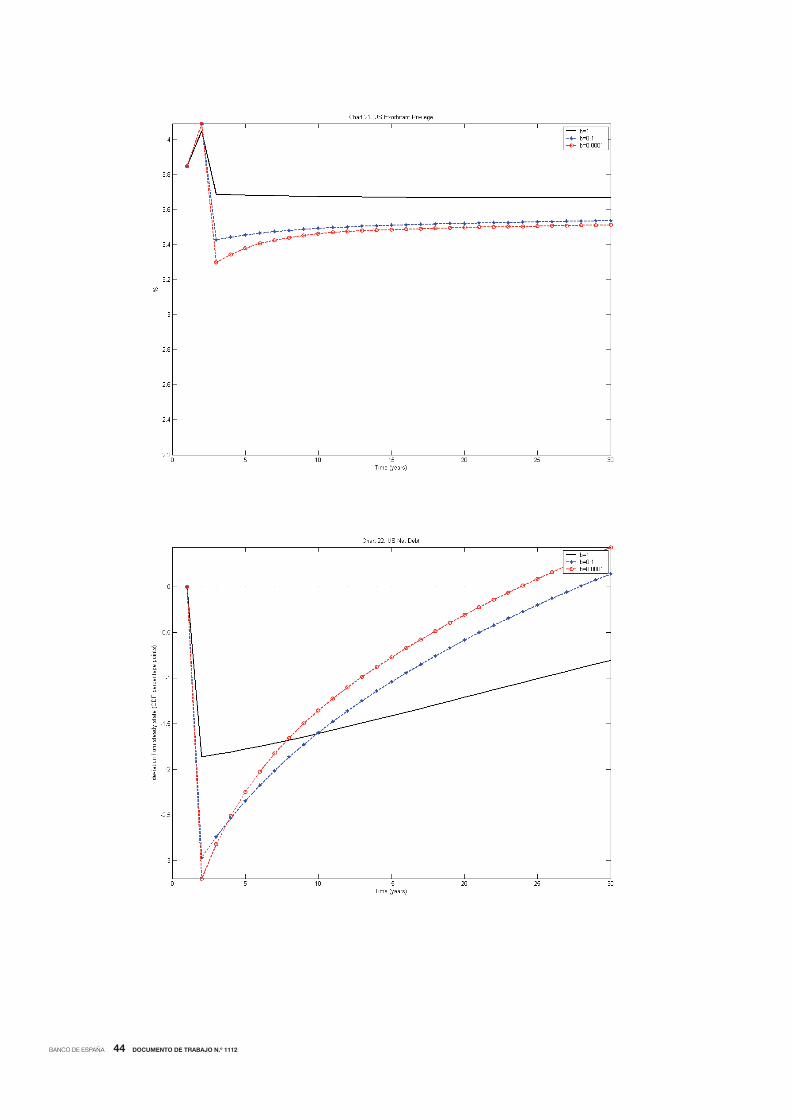
BANCO DE ESPAÑA 44 DOCUMENTO DE TRABAJO N.º 1112
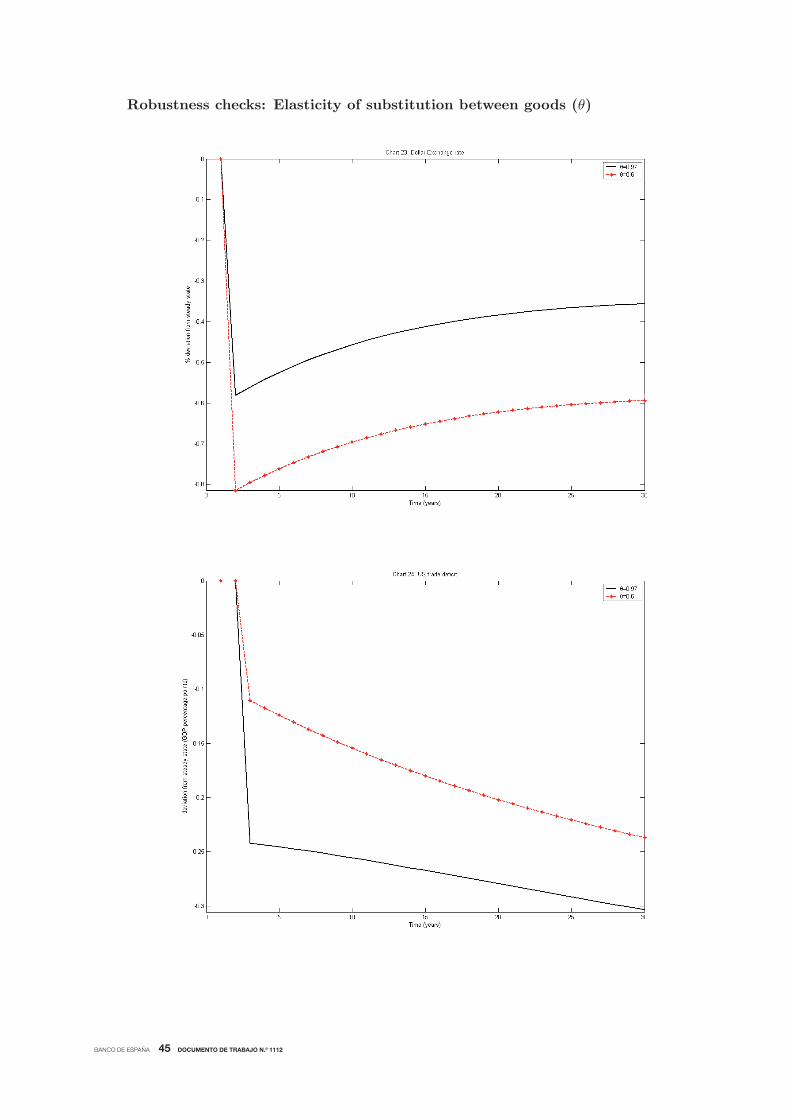
BANCO DE ESPAÑA 45 DOCUMENTO DE TRABAJO N.º 1112
Robustness checks: Elasticity of substitution between goods (θ)

BANCO DE ESPAÑA 46 DOCUMENTO DE TRABAJO N.º 1112
Chart 26. Net foreign purchases of US long-term securities by type
-60000
-40000
-20000
0
20000
40000
60000
80000
100000
120000
140000
2006
-01
2006
-03
2006
-05
2006
-07
2006
-09
2006
-11
2007
-01
2007
-03
2007
-05
2007
-07
2007
-09
2007
-11
2008
-01
2008
-03
2008
-05
2008
-07
2008
-09
2008
-11
2009
-01
2009
-03
2009
-05
2009
-07
2009
-09
2009
-11
2010
-01
2010
-03
2010
-05
2010
-07
2010
-09
$ m
illio
ns
Government bonds Corporate bonds Corporate stocks
Source: US Treasury International Capital System (TIC) data

BANCO DE ESPAÑA 47 DOCUMENTO DE TRABAJO N.º 1112
Table 1. Currency and asset composition of the portfolios of central banks and SWFs
Central Banks SWFsCurrency compositionUSD 60% 38%Other 40% 62%
Asset compositionEquities 0% 71%Bonds 100% 29%
Sources: Data on the currency composition of central banks’ reserves is from the IMF COFER data set (numbers for developing countries). Data on the currency and asset composition of SWFs’ portfolios are from IMF (2008a).
Table 2. Parameter values
Parameter Value SourcePortfolio shares Authors’ calculations in the
appendixShare of US wealth invested in the US market
0.6
Share of ROW wealth invested in the ROW market
* 0.74
Share of US wealth in the US market allocated to equities
0.84
Share of ROW wealth in ROW market allocated to equities
* 0.86
Share of US wealth in ROW market allocated to equities
0.56
Share of ROW wealth in the US market allocated to equities
* 0.31
Rates of return Forbes (2010)Rate of return on US equities rE 1.067
Rate of return on ROW equities rE* 1.124
Rate of return on US bonds rB 1.046
Rate of return on ROW bonds rB* 1.049
Other parametersUS home bias in goods 0.7 Obstfeld and Rogoff (2005)

BANCO DE ESPAÑA 48 DOCUMENTO DE TRABAJO N.º 1112
US capital share 0.39 OECD, Annual National Accounts
ROW capital share * 0.39
Elasticity of substitution between goods 0.97 Hooper and Marquez (1995)
Depreciation rate 0.05 Meredith (2007)
Installation cost of capital 6 Ghosh (2007)
Degree of substitutability between assets b 1 Blanchard, Giavazzi, and Sá (2005)
US productivity A 1 Normalisation
Exchange rate E 1 Normalisation
US net debt to GDP ratio F/Y 0.17 BEA (2008) and IMF International Financial Statistics (IFS)
US consumption to GDP ratio C/Y 0.9 World Bank World Development Indicators (WDI)
ROW consumption to US GDP ratio C*/Y 2.08 WDI
Share of entrepreneurs in US economy E 0.2
Share of entrepreneurs in ROW economy E* 0.2
Relative wealth of entrepreneurs in US economy
VE/VP 0.2
Relative wealth of entrepreneurs in ROW economy
VE*/VP* 0.2
Relative size of US population n 0.05 US Census Bureau
Table 3. Decomposition of the US exorbitant privilege
Our calibration Gourinchas and Rey (2007)Total 3.85% 3.32%Return effect 2.65% 2.45%Composition effect 1.2% 0.86%Source: Authors’ calculations.

BANCO DE ESPAÑA 49 DOCUMENTO DE TRABAJO N.º 1112
Table 4. Path 1 (Currency diversification) – Effect on the US exorbitant privilege
Initial calibration Initial impact (at T=1) Long-run impact (at T=100)Exorbitant privilegeTotal 3.85% 4.05% 3.7%Return effect 2.65% 2.82% 2.5%Composition effect 1.2% 1.23% 1.2%
Source: Authors’ calculations.
Table 5. Path 2 (Asset diversification) – Effect on the US exorbitant privilege
Initial calibration Initial impact (at T=1) Long-run impact (at T=100)Exorbitant privilegeTotal 3.85% 3.72% 3.8%Return effect 2.65% 2.5% 2.7%Composition effect 1.2% 1.22% 1.1%
Source: Authors’ calculations.

BANCO DE ESPAÑA PUBLICATIONS
WORKING PAPERS1
1001 JAVIER ANDRÉS, ÓSCAR ARCE AND CARLOS THOMAS: Banking competition, collateral constraints and optimal
monetary policy.
1002 CRISTINA BARCELÓ AND ERNESTO VILLANUEVA: The response of household wealth to the risk of losing the job:
evidence from differences in firing costs.
1003
1004
ALEXANDER KARAIVANOV, SONIA RUANO, JESÚS SAURINA AND ROBERT TOWNSEND: No bank, one bank,
several banks: does it matter for investment?
GABRIEL PEREZ-QUIROS AND HUGO RODRÍGUEZ MENDIZÁBAL: Asymmetric standing facilities: an unexploited
monetary policy tool.
1005
1006
1007
1008
GABRIEL JIMÉNEZ, JOSE A. LOPEZ AND JESÚS SAURINA: How does competition impact bank
risk-taking?
GIUSEPPE BERTOLA, AURELIJUS DABUSINSKAS, MARCO HOEBERICHTS, MARIO IZQUIERDO, CLAUDIA
KWAPIL, JEREMI MONTORNÈS AND DANIEL RADOWSKI: Price, wage and employment response to shocks:
evidence from the WDN Survey.
JAVIER MENCÍA: Testing non-linear dependence in the Hedge Fund industry.
ALFREDO MARTÍN-OLIVER: From proximity to distant banking: Spanish banks in the EMU.
1009 GALO NUÑO: Optimal research and development expenditure: a general equilibrium approach.
1010
1011
1012
1013
1014
1015
LUIS J. ÁLVAREZ AND PABLO BURRIEL: Is a Calvo price setting model consistent with micro price data?
JENS HAGENDORFF, IGNACIO HERNANDO, MARÍA J. NIETO AND LARRY D. WALL: What do premiums paid for
bank M&As reflect? The case of the European Union.
DAVID DE ANTONIO LIEDO: General equilibrium restrictions for dynamic factor models.
JAMES COSTAIN, JUAN F. JIMENO AND CARLOS THOMAS: Employment fluctuations in a dual labor market.
LUIS M. VICEIRA AND RICARDO GIMENO: The euro as a reserve currency for global investors.
PALOMA LÓPEZ-GARCÍA AND JOSÉ MANUEL MONTERO: Understanding the Spanish business innovation gap:
The role of spillovers and firms' absorptive capacity.
1016
1017
1018
1019
1020
1021
1022
1023
1024
1025
1026
1027
1028
1029
1030
1031
AITOR LACUESTA AND SERGIO PUENTE: El efecto del ciclo económico en las entradas y salidas de inmigrantes
en España.
REBEKKA CHRISTOPOULOU, JUAN F. JIMENO AND ANA LAMO: Changes in the wage structure in EU countries.
THOMAS BREUER, MARTIN JANDAČKA, JAVIER MENCÍA AND MARTIN SUMMER: A systematic approach to
multi-period stress testing of portfolio credit risk.
LUIS J. ÁLVAREZ AND PABLO BURRIEL: Micro-based estimates of heterogeneous pricing rules: The United States
vs. the euro area.
ALFREDO MARTÍN-OLIVER AND VICENTE SALAS-FUMÁS: I.T. investment and intangibles: Evidence from banks.
LUISA LAMBERTINI, CATERINA MENDICINO AND MARIA TERESA PUNZI: Expectations-driven cycles
in the housing market.
JULIÁN MESSINA, PHILIP DU CAJU, CLÁUDIA FILIPA DUARTE, NIELS LYNGGÅRD HANSEN AND MARIO
IZQUIERDO: The incidence of nominal and real wage rigidity: an individual-based sectoral approach.
ALESSIO MORO: Development, growth and volatility.
LUIS J. ÁLVAREZ AND ALBERTO CABRERO: Does housing really lead the business cycle?
JUAN S. MORA-SANGUINETTI: Is judicial inefficiency increasing the house property market weight in Spain?
Evidence at the local level.
MAXIMO CAMACHO, GABRIEL PEREZ-QUIROS AND PILAR PONCELA: Green shoots in the Euro area. A real
time measure.
AITOR ERCE AND JAVIER DÍAZ-CASSOU: Creditor discrimination during sovereign debt restructurings.
RAFAEL REPULLO, JESÚS SAURINA AND CARLOS TRUCHARTE: Mitigating the pro-cyclicality of Basel II.
ISABEL ARGIMÓN AND JENIFER RUIZ: The effects of national discretions on banks.
GABRIEL JIMÉNEZ, STEVEN ONGENA, JOSÉ-LUIS PEYDRÓ AND JESÚS SAURINA: Credit supply: identifying
balance-sheet channels with loan applications and granted loans.
ENRIQUE MORAL-BENITO: Determinants of economic growth: A Bayesian panel data approach.
1. Previously published Working Papers are listed in the Banco de España publications catalogue.

1032
1033
1034
1035
1036
1037
1038
1039
1101
1102
1103
1104
1105
1106
1107
1108
1109
1110
1111
1112
GABE J. DE BONDT, TUOMAS A. PELTONEN AND DANIEL SANTABÁRBARA: Booms and busts in China's stock
market: Estimates based on fundamentals.
CARMEN MARTÍNEZ-CARRASCAL AND JULIAN VON LANDESBERGER: Explaining the demand for money by non-
financial corporations in the euro area: A macro and a micro view.
CARMEN MARTÍNEZ-CARRASCAL: Cash holdings, firm size and access to external finance. Evidence for
the euro area.
CÉSAR ALONSO-BORREGO: Firm behavior, market deregulation and productivity in Spain.
OLYMPIA BOVER: Housing purchases and the dynamics of housing wealth.
DAVID DE ANTONIO LIEDO AND ELENA FERNÁNDEZ MUÑOZ: Nowcasting Spanish GDP growth in real time: “One
and a half months earlier”.
FRANCESCA VIANI: International financial flows, real exchange rates and cross-border insurance.
FERNANDO BRONER, TATIANA DIDIER, AITOR ERCE AND SERGIO L. SCHMUKLER: Gross capital flows: dynamics
and crises.
GIACOMO MASIER AND ERNESTO VILLANUEVA: Consumption and initial mortgage conditions: evidence from
survey data.
PABLO HERNÁNDEZ DE COS AND ENRIQUE MORAL-BENITO: Endogenous fiscal consolidations.
CÉSAR CALDERÓN, ENRIQUE MORAL-BENITO AND LUIS SERVÉN: Is infrastructure capital productive? A dynamic
heterogeneous approach.
MICHAEL DANQUAH, ENRIQUE MORAL-BENITO AND BAZOUMANA OUATTARA: TFP growth and its determinants:
nonparametrics and model averaging.
JUAN CARLOS BERGANZA AND CARMEN BROTO: Flexible inflation targets, forex interventions and exchange rate
volatility in emerging countries.
FRANCISCO DE CASTRO, JAVIER J. PÉREZ AND MARTA RODRÍGUEZ VIVES: Fiscal data revisions in Europe.
ANGEL GAVILÁN, PABLO HERNÁNDEZ DE COS, JUAN F. JIMENO AND JUAN A. ROJAS: Fiscal policy, structural
reforms and external imbalances: a quantitative evaluation for Spain.
EVA ORTEGA, MARGARITA RUBIO AND CARLOS THOMAS: House purchase versus rental in Spain.
ENRIQUE MORAL-BENITO: Dynamic panels with predetermined regressors: likelihood-based estimation and
Bayesian averaging with an application to cross-country growth.
NIKOLAI STÄHLER AND CARLOS THOMAS: FiMod – a DSGE model for fiscal policy simulations.
ÁLVARO CARTEA AND JOSÉ PENALVA: Where is the value in high frequency trading?
FILIPA SÁ AND FRANCESCA VIANI: Shifts in portfolio preferences of international investors: an application to
sovereign wealth funds.
Unidad de Publicaciones Alcalá 522, 28027 Madrid
Telephone +34 91 338 6363. Fax +34 91 338 6488 E-mail: [email protected]
www.bde.es