Shaw, A. D., Neild, S. A., Wagg, D. J., Weaver, P. M., & Carrella, A. (2013).A nonlinear spring mechanism incorporating a bistable composite plate forvibration isolation. Journal of Sound and Vibration, 332(24), 6265–6275.DOI: 10.1016/j.jsv.2013.07.016

Peer reviewed version

Link to published version (if available):10.1016/j.jsv.2013.07.016

Link to publication record in Explore Bristol ResearchPDF-document

NOTICE: this is the author’s version of a work that was accepted for publication in Journal of Sound andVibration. Changes resulting from the publishing process, such as peer review, editing, corrections, structuralformatting, and other quality control mechanisms may not be reflected in this document. Changes may havebeen made to this work since it was submitted for publication. A definitive version was subsequently published inJournal of Sound and Vibration, [332, 24, (2013)] DOI:10.1016/j.jsv.2013.07.016

University of Bristol - Explore Bristol ResearchGeneral rights

This document is made available in accordance with publisher policies. Please cite only the publishedversion using the reference above. Full terms of use are available:http://www.bristol.ac.uk/pure/about/ebr-terms

A nonlinear spring mechanism incorporating a bistablecomposite plate for vibration isolation

A. D. Shawa,∗, S. A. Neildb, D. J. Waggb, P. M. Weavera, A. Carrellac

aAdvanced Composites Centre for Science and Innovation (ACCIS), University of Bristol,Queen’s Building, Bristol, BS8 1TR, United Kingdom

bDepartment of Mechanical Engineering, University of Bristol, Queen’s Building, Bristol,BS8 1TR, United Kingdom

cLMS International, Researchpark Z1, Interleuvenlaan 68, 3001 Leuven, Belgium

Abstract

The High Static Low Dynamic Stiffness (HSLDS) concept is a design strategy for

a nonlinear anti-vibration mount that seeks to increase isolation by lowering the

natural frequency of the mount whilst maintaining the same static load bearing

capacity. It has previously been proposed that an HSLDS mount could be im-

plemented by connecting linear springs in parallel with the transverse flexure of

a composite bistable plate — a plate that has two stable shapes between which

it may snap. Using a bistable plate in this way will lead to lightweight and

efficient designs of HSLDS mounts. This paper experimentally demonstrates

the feasibility of this idea. Firstly, the quasi-static force-displacement curve of

a mounted bistable plate is determined experimentally. Then the dynamic re-

sponse of a nonlinear mass-spring system incorporating this plate is measured.

Excellent agreement is obtained when compared to theoretical predictions based

on the measured force-displacement curve, and the system shows a greater iso-

lation region and a lower peak response to base excitation than the equivalent

linear system.

Keywords: Vibration Isolation, Nonlinear Dynamics, HSLDS, Bistable,

Composites

∗Corresponding author

Preprint submitted to Journal of Sound and Vibration July 16, 2013

1. Introduction

Vibration isolation is a vital requirement throughout much of engineering

[1], particularly when there is a strong source of vibration such as a motor. It

is frequently required to prevent the transmission of these vibrations to other

elements of the system, for reasons such as passenger comfort, or the protection

of delicate electronic equipment.

A High Static Low Dynamic Stiffness (HSLDS) mount seeks to improve vi-

bration isolation by reducing the natural frequency of the mount and its payload,

whilst maintaining the weight bearing capacity of the mount [2]. In the current

work, a nonlinear spring mass system, with an HSLDS force-displacement rela-

tionship, is subjected to harmonic base excitation and response is compared to

analytical predictions made by [3].

An HSLDS response is often achieved by the parallel connection of linear

springs with a snap-through mechanism providing a region of negative stiff-

ness [4], and this approach is followed here. The snap through element adds the

required nonlinearity to the response, whilst the linear springs stabilise the nega-

tive stiffness region and support the static load [2]. The chosen negative stiffness

device is the transverse displacement of the centre of a composite bistable plate.

Bistable plates of this kind have two stable equilibrium shapes which they may

snap between [5], as shown in Fig. (1) (a) and (c). By holding the plate at the

unstable position between these two equilibria shown in Fig. (1) (b), negative

stiffness is observed, which is used to tailor the force-displacement response.

This approach was proposed by Carrella and Friswell [6]. It is thought that

the use of flexible composite shells instead of potentially complex spring mech-

anisms could lead to lightweight and efficient implementations of the HSLDS

concept.

Isolators that exhibit HSLDS behaviour are numerous in the literature, al-

though the HSLDS term itself is relatively new. Authors such as Winterflood

[7], Virgin and Davis [8], Plaut et al. [9], Santillan [10, 11], DeSalvo [12], Car-

rella et al. [13, 14, 15], Kovacic et al. [16], Zhou and Liu [17], Robertson et al.

2

(a) (b) (c)

Figure 1: The different stages of the transverse force-through of a bistable state. (a) Initial,

approximately singly curved configuration. (b) At mid point of force through the plate is

a saddle shape; this shape is unstable if unconstrained and at this point the force displace-

ment graph has negative slope. (c) Final singly curved configuration with curvature along

perpendicular axis to initial curvature.

[18], and Le and Ahn [19] have all worked on variations of the HSLDS concept.

Furthermore, many HSLDS devices are found in the review of passive vibration

isolation methods by Ibrahim [4]. General analysis of the nonlinear phenomena

encountered by HSLDS mounts including amplitude dependant transmissibility

and jump frequencies, based on Duffing oscillator models are given in [2]. Shaw

et. al. has also recently published an analytical study of the HSLDS, show-

ing the significant effect that subtle differences in the shape of the nonlinear

force displacement relationship can cause, and proposing two nondimensional

parameters, which can characterise many HSLDS systems [3].

The ‘snapping’ response of bistable plates was first reported and analysed by

Hyer [5, 20]. He also proposed that these effects could be exploited for the pur-

pose of actuation, creating a device that could occupy multiple configurations

with no ongoing power consumption. Since then, there has been considerable

interest in bistability, for example many authors have looked towards imple-

menting bistable plates in morphing aerodynamic devices including Diaconu et.

al. [21], Schultz [22], Gatto et. al. [23], Daynes et. al. [24, 25] and Lachenal et.

al. [26].

In the current work, the principal aspect of the bistable plate that is of con-

cern is the response to external loading, particularly within the region between

the plates two stable states. This has previously been considered by Dano and

3

Hyer [27], Potter et. al. [28], Tawfik [29], Diaconu et. al. [30], Pirrera et. al.

[31] and Shaw et. al. [32]. However, the current work demonstrates that sub-

stantial qualitative differences to the force displacement curves found in these

works may be obtained.

Section 2 of this work proceeds with a description of the bistable plate, how

it was mounted, and its experimentally derived nonlinear force-displacement

curve. Section 3 then describes how this apparatus was incorporated into a

mechanism with an HSLDS response, and the dynamic experiment that was

conducted. Section 4 gives a theoretical summary of the key static and dynamic

features of an HSLDS mount, and Section 5 compares the experimental results

with theory. Conclusions are drawn in Section 6.

4

Figure 2: The assembled quasi-static test rig. Inset shows detail of one of the spherical pivot

joints used to mount corners.

2. Quasi-static response of the mounted bistable plate subjected to

transverse centre loading

2.1. Bistable plate

A composite bistable plate is typically created on flat tooling by using a

stacking sequence of unidirectional carbon fibre reinforced plastic (CFRP) plies

that is asymmetric about the midplane of the plate. The directional thermal

expansion properties of the plies cause the plate to warp as it cools from its cure

temperature to room temperature, and nonlinear geometrical effects cause the

snapping phenomenon [20].

Hybrid composite bistable plates, consisting of CFRP and steel ply layers,

have been shown to give much greater snapping forces than all CFRP plates [33].

5

To allow a more compact configuration, this type of plate is used here. The layup

and dimensions were chosen to give relatively low curvature in each bistable

state, to prevent the plate forming ‘half-snap’ states during snap-through as re-

ported in [28, 31, 30, 32], which would cause an undesired non-smooth response.

The selected configuration was a 110 mm square plate with a layup [03CF , 01S

, 903CF ] , where the subscripts indicate the number of plies along with CF

for plies of IM7/8552 Intermediate Modulus Carbon Fibre pre-preg nominally

0.125 mm thick, and S for a steel ply 0.25 mm thick. The steel ply was lightly

abraded to improve ‘wetting’ properties and thereby enhance its bonding with

the pre-preg layers. It was vacuum bagged using a tool plate on both sides,

to ensure the most symmetrical resin distribution through thickness. It was

cured using the manufacturers recommended cycle in an autoclave at 180C for

2 hours. Holes 12 mm in diameter were drilled 10 mm in from each corner, to

accommodate pivot joints described below.

2.2. Mounting mechanism

The plate was supported by its corners, on apparatus designed to provide

boundary conditions which do not restrain the snap through. These corner

boundary conditions are vertical pins i.e they allow free out of plane rotation,

zero vertical displacement and free lateral translation. To achieve the first

of these conditions, the corners were fitted with spherical bearings that were

bonded into the 12 mm holes drilled through the plate, that permitted pivoting

in any direction. The plate was clamped flat for the bonding of the pivot joints,

so that the glue fillets did not set into the shape of either stable configuration.

To simultaneously achieve the second and third boundary conditions, the bear-

ings were mounted on tall slender steel posts (approximately 250 mm long, 3

mm in diameter), which were rigidly attached to an adjustable base. Clearly a

more compact mounting would be desirable in a practical design, but this would

cause some compromise to the ideal boundary conditions sought here for the

purpose of establishing feasibility. Vertically the posts provided stiffness greatly

in excess of the plate’s transverse stiffness, and could withstand sufficient buck-

6

−4 −3 −2 −1 0 1 2 3 4−20

0

20

40

60

z (mm)

For

ce (

N)

(a)

−4 −3 −2 −1 0 1 2 3 4−40

−20

0

20

z (mm)

Stif

fnes

s (N

/mm

)

(b)

−0.5 0 0.5

−26

−24

−22

Figure 3: (a) Force-displacement response for plate mounting. Solid lines show results from

quasi-static force-displacement test. Dotted lines show fitted function. Dot-dashed line shows

offset axis about which response is approximately an odd function. (b) Stiffness-displacement

response for plate mounting. Dotted lines show fitted function.

ling force. Horizontally, the posts acted as soft cantilever springs, and the size

of lateral motions was not sufficient to cause significant vertical deflections.

2.3. Quasi-static response

The above apparatus was bolted onto an Instron 3343 load tester, with the

centre of the plate bolted to a 1kN load cell. The complete apparatus is shown

in Fig. (2). The displacement cycle applied to the plate consisted of increasing

displacement at constant velocity over a range including both stable positions

of the plate, then returning at the same speed to the starting point. This was

performed 4 times to ensure repeatability, at a speed of 6 mm/min. Fig. (3) (a)

shows the results of the quasi-static test. There is a small amount of hysteresis in

each cycle, which we believe are caused by frictional moments within the corner

bearings. There is also a large asymmetry in the cycle; the maximum positive

7

force is greater in magnitude than the minimum negative force. This asymmetry

is caused by stresses locked in by the adhesive fillets used to attach the corner

joints, and other manufacturing imperfections. The asymmetry takes the form

of a vertical offset; the dot-dashed line in the graph at F=13.5 N illustrates the

line around which the response is approximately an odd function, as required

by our HSLDS analysis.

Ignoring hysteresis and correcting for the vertical offset, the response may

be fitted with the following function:

F (z) = Az −B arctan(Cz) (1)

where A = 41.9, B = 133.3 and C = 0.507. The coefficients are found by

solving such that the displacement at the zero crossings, the peak force, and the

displacement at peak force match graph readings. As the dotted line in Fig. (3)

(a) shows, this gives a good representation of the central shape of the data.

For dynamic purposes, the stiffness-displacement profile is often of greater

concern than the force-displacement profile. Fig. (3) (b) shows the stiffness-

displacement profile, calculated by numerically differentiating the force-displacement

data with regard to displacement. An undesirable spike occurs at approximately

z=0.5 mm. This is caused by a small degree of freeplay within one of the

spherical joints causing a discontinuity as their loading changes sign. Eq. (1)

differentiates todF

dz= A− BC

C2z2 + 1(2)

and, as can be seen in Fig. (3) (b), this shows agreement with the stiffness data.

It is of note that the force-displacement shown here is fitted by the smooth

function of Eq. (1), and is therefore quite unlike the complex, multi-event re-

sponses reported previously by Potter [28], Pirrera [31], Diaconu [30] and Shaw

[32]. Although the numerous attachments to the plate will clearly influence its

response, the multi-event snap is reproduced in [32] using a very similar method,

so the change in behaviour may be attributed to the different choice of plate

properties.

8

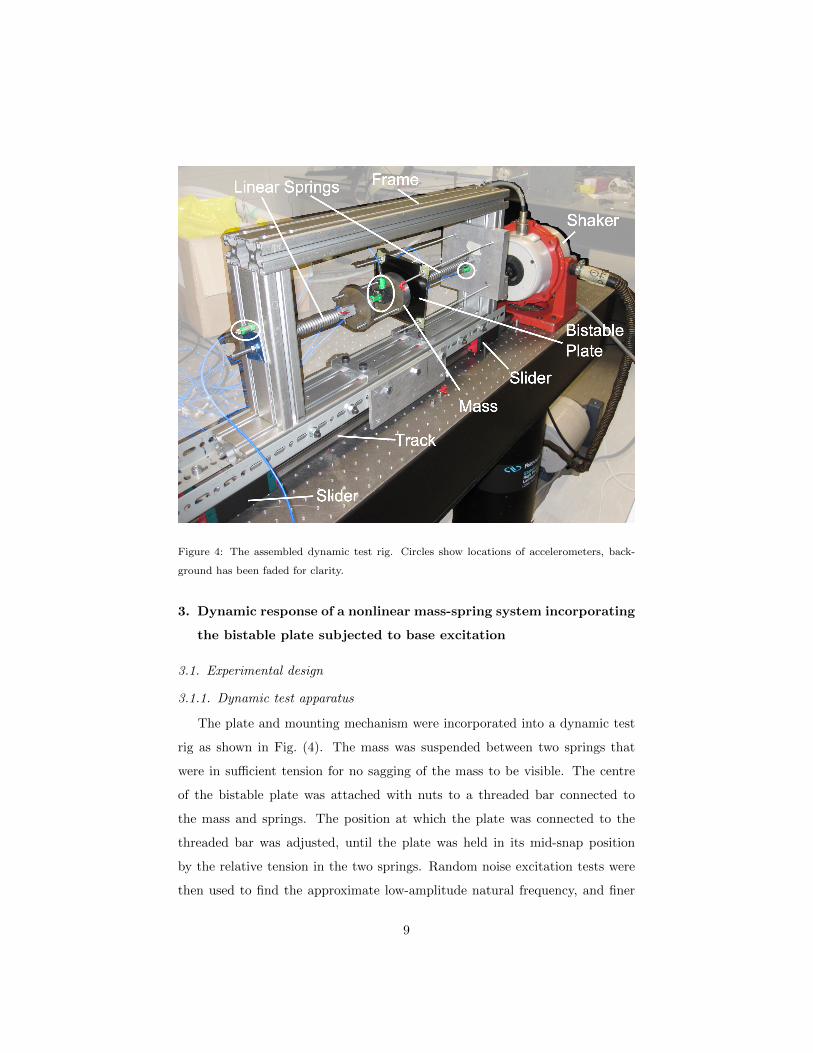
Figure 4: The assembled dynamic test rig. Circles show locations of accelerometers, back-

ground has been faded for clarity.

3. Dynamic response of a nonlinear mass-spring system incorporating

the bistable plate subjected to base excitation

3.1. Experimental design

3.1.1. Dynamic test apparatus

The plate and mounting mechanism were incorporated into a dynamic test

rig as shown in Fig. (4). The mass was suspended between two springs that

were in sufficient tension for no sagging of the mass to be visible. The centre

of the bistable plate was attached with nuts to a threaded bar connected to

the mass and springs. The position at which the plate was connected to the

threaded bar was adjusted, until the plate was held in its mid-snap position

by the relative tension in the two springs. Random noise excitation tests were

then used to find the approximate low-amplitude natural frequency, and finer

9

adjustments were made to these nuts to minimise this frequency, indicating that

the plate was held at the point of minimum stiffness. Locking nuts were then

used to minimise any possible shifting of threaded components during prolonged

vibratory tests.

The outer frame slid upon cars on the steel track, which allowed no de-

tectable rotation or lateral free play, whilst giving minimal axial friction. The

frame was connected to a Ling V406 Shaker, by a connection which included

a short laterally flexible element, which eliminated issues arising from small

misalignments between the shaker and track.

The frame was designed to be far more rigid than the enclosed spring system;

random noise tests were used to verify that no frame modes occurred within the

frequency range of interest, and during testing accelerometers measured both

the top and bottom of the frame, to ensure it was moving as a rigid body.

Two more accelerometers were located on the mass, to check that no significant

lateral motions occurred.

The combined stiffness of the linear springs kspring was estimated as 33.8

N/mm by observing the natural frequency f of the mass-spring system with the

plate decoupled, using 2πf =√kspring/m with effective mass m = 0.97 kg.

3.1.2. Conditioning of the input signal

It was found that the nonlinearities in the system could influence the motion

of the base, and cause distortions to the desired harmonic oscillation. For this

reason, DSpace software and hardware and a Simulink R© model were used to

develop a control system that could minimise these unwanted harmonics. A

feed-forward system was used in preference to a feedback control system, to

avoid potential issues of instability. The controller repeatedly sampled a buffer

of data from the base accelerometer, then calculated the Fourier series of this

signal based upon the required fundamental frequency, including terms up to

the 5th harmonic. A numerical routine was run that assumed that the mag-

nitude of each harmonic of the base signal was an unknown function of the

output Fourier coefficients at the same harmonic, and used a Newton-Broyden

10

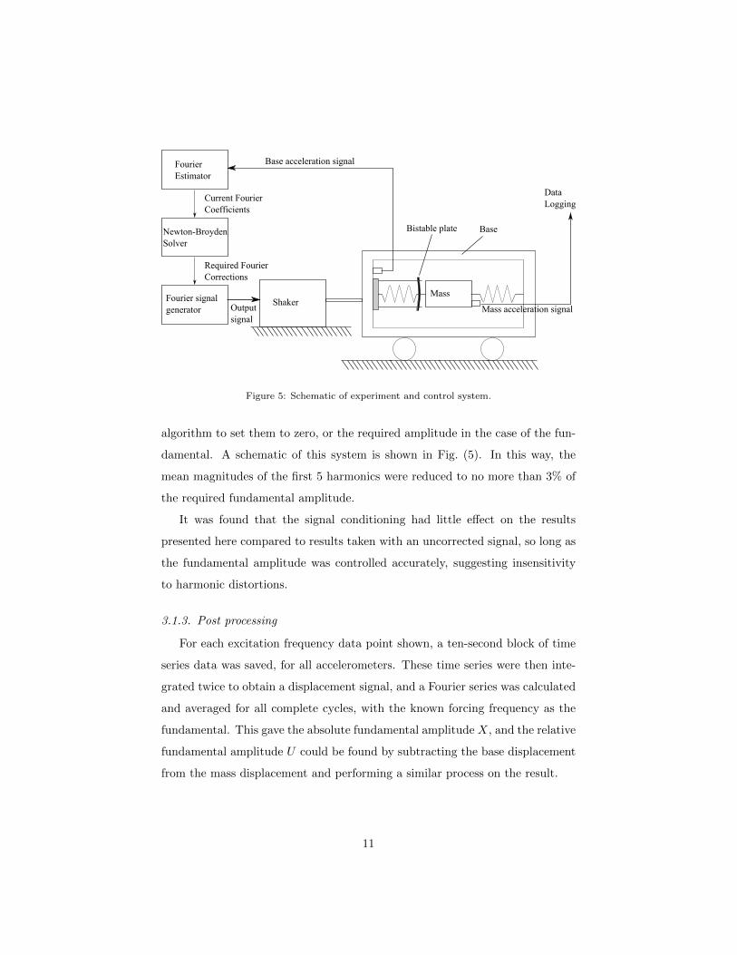
Base

FourierEstimator

Newton-BroydenSolver

Fourier signalgenerator

MassShaker

Current Fourier Coefficients

Required Fourier Corrections

Outputsignal

Base acceleration signal

DataLogging

Mass acceleration signal

Bistable plate

Figure 5: Schematic of experiment and control system.

algorithm to set them to zero, or the required amplitude in the case of the fun-

damental. A schematic of this system is shown in Fig. (5). In this way, the

mean magnitudes of the first 5 harmonics were reduced to no more than 3% of

the required fundamental amplitude.

It was found that the signal conditioning had little effect on the results

presented here compared to results taken with an uncorrected signal, so long as

the fundamental amplitude was controlled accurately, suggesting insensitivity

to harmonic distortions.

3.1.3. Post processing

For each excitation frequency data point shown, a ten-second block of time

series data was saved, for all accelerometers. These time series were then inte-

grated twice to obtain a displacement signal, and a Fourier series was calculated

and averaged for all complete cycles, with the known forcing frequency as the

fundamental. This gave the absolute fundamental amplitude X, and the relative

fundamental amplitude U could be found by subtracting the base displacement

from the mass displacement and performing a similar process on the result.

11

10 15 20 25 300

0.5

1

Am

plitu

de (

mm

)

Frequency (Hz)

(a)

10 15 20 25 300

0.5

1

Am

plitu

de (

mm

)

Frequency (Hz)

(b)

10 15 20 25 300

0.5

1

1.5

Am

plitu

de (

mm

)

Frequency (Hz)

(c)

10 15 20 25 300

0.5

1

1.5

Am

plitu

de (

mm

)

Frequency (Hz)

(d)

Figure 6: Fundamental absolute response amplitude for different values of base amplitude R

and frequency. Crosses (+) show experimental data, peak values shown with (×××), line shows

response calculated in Section 5.3 with dots indicating unstable response regions. (a) R = 0.04

mm (b) R = 0.05 mm (c) R = 0.06 mm (d) R = 0.07 mm

12

3.2. Dynamic results

Fig. (6) shows detailed frequency response results at each of the four exci-

tation amplitudes tested. Each point represents a steady state response at the

frequency shown. Each set of data consists of three batches of readings. Firstly

a sequence of points was taken at increasing frequencies at intervals of approx

2.5Hz to get a ‘feel’ for the overall response. This was followed by a set of

points taken at refined frequency intervals at progressively lower frequencies to

resolve the lower frequency bound of the unstable response region, known as the

‘jump-up’ frequency [2]. Finally, readings were taken at increasing frequencies

at refined intervals to resolve the upper branch and peak region of the response.

The entire data set took approximately two working days to collect, due to the

time taken for the input signal conditioning to achieve a settled, harmonic in-

put signal. Over the course of this time, some loss of the adjustment made in

Section 3.1.1 seems to have occurred leading to some scatter in results; results

taken shortly after one another showed excellent repeatability.

13

m

cPk(z)

x(t)

r(t)

Fs

Figure 7: Massm with static load Fs is supported on a movable base by a nonlinear spring with

linear damper with damping constant c. r(t) denotes base motion, x(t) denotes displacement

response of the mass and the nonlinear spring has force/displacement function Pk(z).

4. Static and dynamic analysis of an HSLDS mount

To model the results, we provide a brief theoretical description of the HSLDS

mount, summarising recent work by the authors [3]. Fig. (7) shows the system

considered; a mass m subject to static load Fs is supported above a base by

a nonlinear spring with force/displacement response Pk(z) and linear damper

with coefficient c. It is excited by base excitation signal r(t), resulting in an

absolute displacement from the static equilibrium position x(t). Inspection of

Fig. (7) gives the following equation of motion:

mz + cz + P (z) = mr (3)

where z ≡ x(t) − r(t) and is known as relative displacement, and P (z) = Fs −

Pk(z) describes restoring force. It is assumed that x = r = z = 0 at static

equilibrium.

An HSLDS function for the nonlinear spring P (z) is an odd function similar

in form to Fig. (8) (a). Stiffness is low near the origin, giving reduced natural

frequency at small amplitudes, while greater stiffness elsewhere minimises the

deflection due to Fs. The equivalent linear system is defined as the linear system

that has the same static displacement zs at the given static load Fs, with conse-

quent static stiffness ks ≡ Fs/zs. Distance and force are nondimensionalised by

14

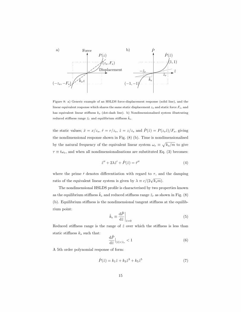
(−1,−1)

P (z)

(1, 1)

z

Pb)

zr−zr

ke

P (z)

(zs, Fs)

ksz

Displacement

Forcea)

(−zs,−Fs)

Figure 8: a) Generic example of an HSLDS force-displacement response (solid line), and the

linear equivalent response which shares the same static displacement zs and static force Fs, and

has equivalent linear stiffness ks (dot-dash line). b) Nondimensionalised system illustrating

reduced stiffness range zr and equilibrium stiffness ke.

the static values; x = x/zs, r = r/zs, z = z/zs and P (z) = P (zsz)/Fs, giving

the nondimensional response shown in Fig. (8) (b). Time is nondimensionalised

by the natural frequency of the equivalent linear system ωe ≡√ks/m to give

τ ≡ tωe, and when all nondimensionalisations are substituted Eq. (3) becomes:

z′′ + 2λz′ + P (z) = r′′ (4)

where the prime ′ denotes differentiation with regard to τ , and the damping

ratio of the equivalent linear system is given by λ ≡ c/(2√ksm).

The nondimensional HSLDS profile is characterised by two properties known

as the equilibrium stiffness ke and reduced stiffness range zr as shown in Fig. (8)

(b). Equilibrium stiffness is the nondimensional tangent stiffness at the equilib-

rium point:

ke ≡dP

dz

∣∣∣∣z=0

(5)

Reduced stiffness range is the range of z over which the stiffness is less than

static stiffness ks such that:dP

dz

∣∣|z|<zr

< 1 (6)

A 5th order polynomial response of form:

P (z) = k1z + k3z3 + k5z

5 (7)

15

X

Ω0 0.2 0.4 0.6 0.8 1 1.20

0.1

0.2

0.3

0.4

0.5

0.6

0.7

0.8

0.9

1

Figure 9: Typical absolute steady state frequency response functions for an HSLDS mount,

ke = 0.5, zr = 0.5, λ = 0.025, R = 0.0375. The right hand peak shows the response of

the equivalent linear system for comparison. The dashed line shows the limit curve for the

applied base excitation amplitude and damping, the dot-dash lines show backbone curves.

Dots indicate unstable regions of response.

can be fitted to match the condition that P (1) = 1, and solved to satisfy Eq. (5)

and Eq. (6) to obtain:

k1 = ke , k3 = (1− ke)5z4r − 1

5z4r − 3z2r, k5 = (1− ke)

1− 3z2r5z4r − 3z2r

(8)

Equilibrium stiffness may be in the range 0 < ke ≤ 1, where a value of 1 gives a

purely linear system. The reduced stiffness range must be restricted to√

1/5 ≤

zr ≤ 4√

1/5 for the fifth order model; a value of zr outside of this range can result

in an excessively complex shape for the response that is unlikely to represent

a physical system, and may feature regions of negative stiffness [3]. Dynamic

simulation shows that for non-polynomial HSLDS functions, approximating the

force-displacement curve using equations (5) to (8) gives very similar results [3].

To obtain the steady state response to harmonic base motion of the form

r = R cos(Ωτ + φ), the method of Normal Forms [34, 35] is used in [3], however

the Harmonic Balance method [36] would give identical results in this case.

The method of Normal Forms assumes a relative response of the form z =

16

U cos(Ωτ) + h(τ), where h(τ) is a small function containing harmonic responses

that is neglected in this work. This results in a response equation that may be

solved to find U , the amplitude of the response at the forcing frequency :

Ω4(U2 − R2) + 2Ω2U2[2λ2 −K(U)

]+K(U)2U2 = 0 (9)

where K(U) is the amplitude dependant stiffness:

K(U) = ke +3k3U

2

4+

10k5U4

16(10)

It may be shown that in some cases the solutions given by Eq. (9) are not

dynamically stable, for example by Xin et. al. [37], and these unstable cases lie

on the underside of the nonlinear peak as shown by dots in Fig. (9).

When forcing and damping are assumed to be zero, Eq. (9) defines the

amplitude dependant natural frequency of the system, known as the backbone

curve:

Ω =

√K(U) (11)

At resonance, stiffness and inertial terms cancel from Eq. (9) to give:

U =ΩR

2λ(12)

which is known as the limit curve. The peak response for any given nonlinear

spring occurs when its backbone curve intersects the limit curve for the relevant

base amplitude and damping.

We are often primarily concerned with the absolute response of the pay-

load mass. The nondimensional absolute fundamental magnitude X may be

calculated from the relative magnitude U by

X =

√(U + R cosφ)2 + (R sinφ)2 (13)

where φ is the phase angle between the base motion and relative response given

by

φ = cos−1

((−Ω2 +K(U))U

Ω2R

)(14)

17

Eqns. (11) and (12) concern a system that is in resonance, so therefore φ = π/2

and U >> R, and the effect of R becomes negligible in Eq. (13) so that U ≈ X.

Therefore limit curves and backbone curves are identical when plotted in terms

of relative or absolute response, except at very low frequencies where X → R.

An example response is shown in Fig. (9), showing that the use of an HSLDS

mount reduces both the peak frequency and the peak amplitude of response to

base excitation. Note that at low frequency, the absolute response magnitude

converges to the base motion amplitude. Fig. (9) shows that the region where

absolute response magnitude is less than that of the base magnitude, known as

the isolation region, begins at much lower frequency for the HSLDS mount than

for the equivalent linear system.

5. Comparison of Experimental Data with Theory

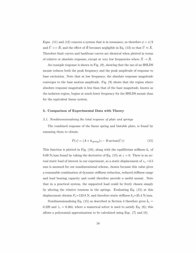
5.1. Nondimensionalising the total response of plate and springs

The combined response of the linear spring and bistable plate, is found by

summing them to obtain:

P (z) = (A+ kspring)z −B arctan(Cz) (15)

This function is plotted in Fig. (10), along with the equilibrium stiffness ke of

8.09 N/mm found by taking the derivative of Eq. (15) at z = 0. There is no ac-

tual static load of interest in our experiment, so a static displacement of zs =3.5

mm is assumed for our nondimensional scheme, chosen because this value gives

a reasonable combination of dynamic stiffness reduction, reduced stiffness range

and load bearing capacity and could therefore provide a useful mount. Note

that in a practical system, the supported load could be freely chosen simply

by altering the relative tensions in the springs. Evaluating Eq. (15) at this

displacement obtains Fs=123.8 N, and therefore static stiffness ks=35.4 N/mm.

Nondimensionalising Eq. (15) as described in Section 4 therefore gives ke =

0.229 and zr = 0.464, where a numerical solver is used to satisfy Eq. (6); this

allows a polynomial approximation to be calculated using Eqs. (7) and (8).

18

−4 −3 −2 −1 0 1 2 3 4−150

−100

−50

0

50

100

150

z (mm)

P (

N)

Figure 10: Total force displacement function given by Eq. (15) (solid). Dotted line gradient

shows equilibrium stiffness, dot-dashed line shows equivalent linear system. Crosses indicate

chosen static displacement and consequent static force.

5.2. Comparison of Backbone curves

Fig. (11) shows all result sets shown in Fig. (6) nondimensionalised as de-

scribed in Sections 4 and 5.1. Three backbone curves are shown in bold; the

dot-dashed backbone is calculated using Eqs. (8), (10) and (11) with the values

of ke and zr calculated for Eq. (15) in Section 5.1. As can be seen, this curve has

a qualitatively similar shape to the data but is inaccurate in terms of frequency.

The reason for this is found by inspecting the inset in Fig. (3) (b) at z=0 mm;

there is a range of approximately 2 N/mm in the data, and this is a significant

proportion of the dimensional equilibrium stiffness, which is calculated to be

8.09 N/mm. Furthermore, it is likely that there is some error in adjusting the

plate so that it is held at its exact centre. Therefore it is difficult to establish

the true equilibrium stiffness value with accuracy. A value for the stiffness of

the plate at z=0 mm of -23.5 N/mm, which Fig. (3) shows occurs inside a range

of 0.5 mm from zero, gives a dimensional stiffness of 10.3 N/mm when summed

with the spring stiffness. Nondimensionalising by the calculated static stiffness

gives ke = 0.291, and this value in Eqs. (8), (10) and (11) gives the solid back-

bone curve in Fig. (11) which fits the data well. Finally, the dotted backbone

curve shown in Fig. (11) shows the response if the model is simply taken to be a

cubic polynomial with the same equilibrium stiffness, showing that this model

19

0 0.1 0.2 0.3 0.4 0.5 0.6 0.7 0.8 0.9 10

0.1

0.2

0.3

0.4

0.5

X

Ω

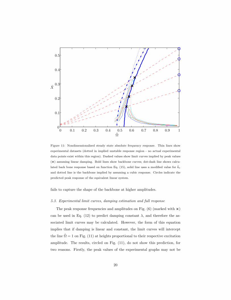
Figure 11: Nondimensionalised steady state absolute frequency response. Thin lines show

experimental datasets (dotted in implied unstable response region - no actual experimental

data points exist within this region). Dashed values show limit curves implied by peak values

(×××) assuming linear damping. Bold lines show backbone curves; dot-dash line shows calcu-

lated back bone response based on function Eq. (15), solid line uses a modified value for ke

and dotted line is the backbone implied by assuming a cubic response. Circles indicate the

predicted peak response of the equivalent linear system.

fails to capture the shape of the backbone at higher amplitudes.

5.3. Experimental limit curves, damping estimation and full response

The peak response frequencies and amplitudes on Fig. (6) (marked with ×××)

can be used in Eq. (12) to predict damping constant λ, and therefore the as-

sociated limit curves may be calculated. However, the form of this equation

implies that if damping is linear and constant, the limit curves will intercept

the line Ω = 1 on Fig. (11) at heights proportional to their respective excitation

amplitude. The results, circled on Fig. (11), do not show this prediction, for

two reasons. Firstly, the peak values of the experimental graphs may not be

20

entirely accurate; when response has a ‘drop-down’, it is not possible to know

exactly how near to the true peak frequency was reached before the drop-down

was triggered. Secondly, there is no physical reason for the assumption of lin-

ear damping, so some amplitude dependence may be occurring. The physical

sources of damping in composites are complex [38], and amplitude dependence

has been demonstrated in dynamic tests on simple carbon composites [39], al-

though no damping data currently exists for hybrid bistable laminates. Other

details of the test rig may also introduce nonlinear dissipation, such as the

spherical bearings at the corners of the plate which may incur some freeplay

and frictional nonlinearity during vibration [36].

Nevertheless, the above method is used to calculate values of λ separately

for each different level of forcing. The solutions of Eq. (9) can then be found,

converted to absolute response with Eq. (13), and plotted in dimensional form

as solid lines on Fig. (6). This shows good agreement with experiment.

21

6. Conclusions

An experimental concept demonstrator for a passive vibration isolator in-

corporating a composite bistable plate has been built, and subjected to har-

monic base excitation. Quasi-static tests have been performed to characterise

the force-displacement properties of the snap through of the bistable plate, and

the results used to make predictions for the dynamic response of a spring-mass

system coupled with this plate.

The quasi-static results show that the force through of a bistable plate need

not be the complex multi-stage event reported by other authors if a configura-

tion with shallow bistable curvature is used. The resulting plate may be used

in an anti-vibration mechanism that we have shown could support substantial

load whilst reducing the natural frequency of the mounted payload significantly

relative to a linear mount with equivalent static stiffness.

The dynamic results show good agreement with theoretical predictions, in

particular the backbone curve which matches the shape of the frequency re-

sponse function well, although it proved difficult to accurately predict the equi-

librium stiffness due to experimental scatter. Selecting the peak response at a

given amplitude is not a particularly robust way to find the damping ratio of the

system, and the assumption of linear damping could not be verified. However,

deriving the damping ratio in this way and using it in our model to calculate

the response away from the peak still gave reasonably accurate results.

Future work on this will move towards a more compact mounting, with

a view towards achieving a simple, lightweight and highly effective means of

isolating vibration.

Acknowledgements

The authors would like to thank Dr David Barton and Clive Rendall for their

assistance in this project. Alexander Shaw has an EPSRC studentship from

the Advanced Composites Centre for Innovation and Science (ACCIS) Doctoral

22

Training Centre (DTC), grant number EP/G036772/1. Simon Neild is an EP-

SRC research fellow. David Wagg is funded by EPSRC grant EP/K003836/1.

References

[1] D. J. Mead, Passive Vibration Control, John Wiley and Sons, 1999.

[2] A. Carrella, Passive Vibration Isolators with High-Static-Low-Dynamic-

Stiffness, VDM Verlag Dr. Muller, 2010.

[3] A. Shaw, S. Neild, D. Wagg, Dynamic analysis of high static low dynamic

stiffness vibration isolation mounts, Journal of Sound and Vibration 332 (6)

(2013) 1437–1455. doi:10.1016/j.jsv.2012.10.036.

[4] R. Ibrahim, Recent advances in nonlinear passive vibration isolators, Jour-

nal of Sound and Vibration 314 (3-5) (2008) 371 – 452.

[5] M. W. Hyer, Some observations on the cured shape of thin unsymmetric

laminates, Journal of Composite Materials 15 (2) (1981) 175–194.

[6] A. Carrella, M. Friswell, A. Pirrera, G. Aglietti, Numerical and experi-

mental analysis of a square bistable plate, in: International Conference on

Noise and Vibration (ISMA 2008), 2008.

[7] J. Winterflood, D. G. Blair, B. Slagmolen, High performance vibration

isolation using springs in euler column buckling mode, Physics Letters A

300 (2-3) (2002) 122–130.

[8] L. N. Virgin, R. B. Davis, Vibration isolation using buckled struts, Journal

of Sound and Vibration 260 (5) (2003) 965–973.

[9] R. H. Plaut, J. E. Sidbury, L. N. Virgin, Analysis of buckled and pre-

bent fixed-end columns used as vibration isolators, Journal of Sound and

Vibration 283 (3-5) (2005) 1216–1228.

23

[10] L. N. Virgin, S. T. Santillan, R. H. Plaut, Vibration isolation using extreme

geometric nonlinearity, Journal of Sound and Vibration 315 (3) (2008) 721–

731.

[11] S. T. Santillan, Analysis of the elastica with applications to vibration iso-

lation, Ph.D. thesis, Department of Mechanical Engineering and Materials

Science, Duke University (2007).

[12] R. DeSalvo, Passive, nonlinear, mechanical structures for seismic atten-

uation, Journal of Computational and Nonlinear Dynamics 2 (4) (2007)

290–298.

[13] A. Carrella, M. Brennan, T. Waters, Static analysis of a passive vibra-

tion isolator with quasi-zero-stiffness characteristic, Journal of Sound and

Vibration 301 (301) (2007) 678 – 689.

[14] A. Carrella, M. Friswell, A. Zotov, D. Ewins, A. Tichonov, Using nonlinear

springs to reduce the whirling of a rotating shaft, Mechanical Systems and

Signal Processing 23 (7) (2009) 2228 – 2235.

[15] A. Carrella, M. Brennan, T. Waters, V. L. Jr., Force and displace-

ment transmissibility of a nonlinear isolator with high-static-low-dynamic-

stiffness, International Journal of Mechanical Sciences 55 (1) (2012) 22 –

29.

[16] I. Kovacic, M. J. Brennan, T. P. Waters, A study of a nonlinear vibration

isolator with a quasi-zero stiffness characteristic, Journal of Sound and

Vibration 315 (3) (2008) 700 – 711.

[17] N. Zhou, K. Liu, A tunable high-static low-dynamic stiffness vibration

isolator, Journal of Sound and Vibration 329 (9) (2010) 1254 – 1273.

[18] W. S. Robertson, M. R. F. Kidner, B. S. Cazzolato, A. C. Zander, The-

oretical design parameters for a quasi-zero stiffness magnetic spring for

vibration isolation, Journal of Sound and Vibration 1-2 (2009) 88–103.

24

[19] T. D. Le, K. K. Ahn, A vibration isolation system in low frequency exci-

tation region using negative stiffness structure for vehicle seat, Journal of

Sound and Vibration 330 (26) (2011) 6311–6335.

[20] M. W. Hyer, Calculations of the room-temperature shapes of unsymmetric

laminates, Journal of Composite Materials 15 (1981) 296–310.

[21] C. G. Diaconu, P. M. Weaver, F. Mattioni, Concepts for morphing air-

foil sections using bi-stable laminated composite structures, Thin-Walled

Structures 46 (6) (2008) 689 – 701.

[22] M. R. Schultz, A concept for airfoil-like active bistable twisting structures,

Journal of Intelligent Material Systems and Structures 19 (2) (2008) 157–

169.

[23] A. Gatto, F. Mattioni, M. Friswell, Experimental investigation of bistable

winglets to enhance wing lift takeoff capability, Journal of Aircraft 46 (2)

(2009) 647.

[24] S. Daynes, P. Weaver, K. Potter, P. Margaris, P. Mellor, Bistable composite

flap for an airfoil, Journal of Aircraft 47 (2010) 334–338.

[25] S. Daynes, P. Weaver, J. Trevarthen, A morphing composite air inlet with

multiple stable shapes, Journal of Intelligent Material Systems and Struc-

tures 22 (9) (2011) 961–973.

[26] X. Lachenal, S. Daynes, P. M. Weaver, Review of morphing concepts and

materials for wind turbine blade applications, Wind Energy 16 (2) (2013)

283–307. doi:10.1002/we.531.

[27] M. Dano, M. W. Hyer, The response of unsymmetric laminates to sim-

ple applied forces, Mechanics of Composite Materials and Structures 3 (1)

(1996) 65–80.

[28] K. Potter, P. Weaver, A. Seman, S. Shah, Phenomena in the bifurcation

of unsymmetric composite plates, Composites Part A: Applied Science and

Manufacturing 38 (1) (2007) 100 – 106.

25

[29] S. Tawfik, X. Tan, S. Ozbay, E. Armanios, Anticlastic stability modeling

for cross-ply composites, Journal of composite materials 41 (11) (2007)

1325–1338.

[30] C. G. Diaconu, P. M. Weaver, A. F. Arrieta, Dynamic analysis of bi-stable

composite plates, Journal of Sound and Vibration 322 (4-5) (2009) 987 –

1004.

[31] A. Pirrera, D. Avitabile, P. Weaver, Bistable plates for morphing struc-

tures: A refined analytical approach with high-order polynomials, Interna-

tional Journal of Solids and Structures 47 (25-26) (2010) 3412 – 3425.

[32] A. D. Shaw, A. Carrella, Force displacement curves of a snapping bistable

plate, in: Proceedings of the 30th IMAC, A Conference on Structural Dy-

namics, 2012, pp. 191–198.

[33] S. Daynes, P. M. Weaver, Analysis of unsymmetric cfrp-metal hybrid lam-

inates for use in adaptive structures, Composites Part A: Applied Science

and Manufacturing 41 (11) (2010) 1712–1718.

[34] S. A. Neild, D. J. Wagg, Applying the method of normal forms to second-

order nonlinear vibration problems, Proc. R. Soc. A 467 (2128) (2010) 1141

– 1163.

[35] S. A. Neild, Approximate methods for analysing nonlinear structures, in:

L. Virgin, D. Wagg (Eds.), Exploiting Nonlinear Behaviour in Structural

Dynamics, Springer, 2012, pp. 53 – 109.

[36] D. Wagg, S. Neild, Nonlinear Vibration with Control, Springer, 2009.

[37] Z. Xin, S. Neild, D. Wagg, Z. Zuo, Resonant response functions for nonlin-

ear oscillators with polynomial type nonlinearities, Journal of Sound and

Vibration 332 (7) (2013) 1777 – 1788. doi:10.1016/j.jsv.2012.09.022.

[38] R. Chandra, S. Singh, K. Gupta, Damping studies in fiber-reinforced

composites - a review, Composite Structures 46 (1) (1999) 41 – 51.

doi:10.1016/S0263-8223(99)00041-0.

26

[39] R. Adams, M. Maheri, Dynamic flexural properties of anisotropic fibrous

composite beams, Composites Science and Technology 50 (4) (1994) 497 –

514. doi:10.1016/0266-3538(94)90058-2.

List of Figures

1 The different stages of the transverse force-through of a bistable

state. (a) Initial, approximately singly curved configuration. (b)

At mid point of force through the plate is a saddle shape; this

shape is unstable if unconstrained and at this point the force

displacement graph has negative slope. (c) Final singly curved

configuration with curvature along perpendicular axis to initial

curvature. . . . . . . . . . . . . . . . . . . . . . . . . . . . . . . 3

2 The assembled quasi-static test rig. Inset shows detail of one of

the spherical pivot joints used to mount corners. . . . . . . . . . 5

3 (a) Force-displacement response for plate mounting. Solid lines

show results from quasi-static force-displacement test. Dotted

lines show fitted function. Dot-dashed line shows offset axis about

which response is approximately an odd function. (b) Stiffness-

displacement response for plate mounting. Dotted lines show

fitted function. . . . . . . . . . . . . . . . . . . . . . . . . . . . . 7

4 The assembled dynamic test rig. Circles show locations of ac-

celerometers. . . . . . . . . . . . . . . . . . . . . . . . . . . . . . 9

5 Schematic of experiment and control system. . . . . . . . . . . . 11

6 Fundamental absolute response amplitude for different values of

base amplitude R and frequency. Crosses (+) show experimental

data, peak values shown with (×××), line shows response calculated

in Section 5.3 with dots indicating unstable response regions. (a)

R = 0.04 mm (b) R = 0.05 mm (c) R = 0.06 mm (d) R = 0.07

mm . . . . . . . . . . . . . . . . . . . . . . . . . . . . . . . . . . 12

27

7 Mass m with static load Fs is supported on a movable base by

a nonlinear spring with linear damper with damping constant c.

r(t) denotes base motion, x(t) denotes displacement response of

the mass and the nonlinear spring has force/displacement func-

tion Pk(z). . . . . . . . . . . . . . . . . . . . . . . . . . . . . . . 14

8 a) Generic example of an HSLDS force-displacement response

(solid line), and the linear equivalent response which shares the

same static displacement zs and static force Fs, and has equiva-

lent linear stiffness ks (dot-dash line). b) Nondimensionalised sys-

tem illustrating reduced stiffness range zr and equilibrium stiff-

ness ke. . . . . . . . . . . . . . . . . . . . . . . . . . . . . . . . . 15

9 Typical absolute steady state frequency response functions for

an HSLDS mount, ke = 0.5, zr = 0.5, λ = 0.025, R = 0.0375.

The right hand peak shows the response of the equivalent linear

system for comparison. The dashed line shows the limit curve

for the applied base excitation amplitude and damping, the dot-

dash lines show backbone curves. Dots indicate unstable regions

of response. . . . . . . . . . . . . . . . . . . . . . . . . . . . . . 16

10 Total force displacement function given by Eq. (15) (solid). Dot-

ted line gradient shows equilibrium stiffness, dot-dashed line shows

equivalent linear system. Crosses indicate chosen static displace-

ment and consequent static force. . . . . . . . . . . . . . . . . . 19

28

11 Nondimensionalised steady state absolute frequency response. Thin

lines show experimental datasets (dotted in implied unstable re-

sponse region - no actual experimental data points exist within

this region). Dashed values show limit curves implied by peak

values (×××) assuming linear damping. Bold lines show backbone

curves; dot-dash line shows calculated back bone response based

on function Eq. (15), solid line uses a modified value for ke and

dotted line is the backbone implied by assuming a cubic response.

Circles indicate the predicted peak response of the equivalent lin-

ear system. . . . . . . . . . . . . . . . . . . . . . . . . . . . . . . 20

29