sharper symmetric self-hilbertian wavelets

Contents lists available at ScienceDirect

Signal Processing

Signal Processing 98 (2014) 202–211

0165-16http://d

n CorrE-m

s.murug

journal homepage: www.elsevier.com/locate/sigpro

Sharper Symmetric Self-Hilbertian wavelets

David B.H. Tay n, Selvaraaju MurugesanDepartment of Electronic Engineering, LaTrobe University, Bundoora, Victoria 3086, Australia

a r t i c l e i n f o

Article history:Received 4 September 2013Received in revised form21 November 2013Accepted 29 November 2013Available online 8 December 2013

Keywords:Filter banksDual-tree complex waveletHilbert pair

84/$ - see front matter & 2013 Elsevier B.V.x.doi.org/10.1016/j.sigpro.2013.11.040

esponding author.ail addresses: [email protected] (D.B.H. [email protected] (S. Murugesan).

a b s t r a c t

Symmetric Self-Hilbertian (SSH) wavelets are building blocks to many dual-tree complexwavelet transform systems. The SSH wavelets, and the corresponding scaling filters,within a pair are time-reverse versions of each other, and the complex wavelet functionhas conjugate symmetry. Previously reported methods for designing these wavelets focusmainly on achieving the best approximation to the Hilbert transform, where all designparameters are optimized with respect to the analytic quality. The exception is a techniqueproposed by the author (Signal Processing 2012) that allows the control of the frequencyresponse sharpness of the corresponding scaling filter. However the technique is practicalonly when the number of free-parameters is small due to the high computational loadotherwise. This paper proposes novel techniques that are based on the orthogonal latticeand are practical with any number of free-parameters. Higher analytic quality Hilbertpairs with sharper response can be obtained when there are more free-parameters. Threestrategies for optimizing the lattice parameters to give high quality filters are presentedhere.

& 2013 Elsevier B.V. All rights reserved.

1. Introduction

The wavelet transform is now established as an indis-pensable tool for signal representation and is used in avariety of applications [1–3]. Newer generation of waveletsis based on redundant transforms [4,5] and is related tothe theory of frames in mathematics. One of the mostsuccessful redundant wavelet transforms in recent times isthe dual-tree complex wavelet transform (DTCWT) thatwas pioneered by Kingsbury [6], and has been effective ina variety of applications ranging from de-noising to imagemodelling [7,8].

The key component to the implementation of theDTCWT is a pair of perfect reconstruction 2-channelmultirate filter bank. Although as the name suggests theDTCWT is complex, no complex arithmetic is required inits implementation, and the two filter banks are used

All rights reserved.

y),

independently in two tree structures. The filter banks arehowever implicitly related to each other via the Hilberttransform. Specifically the equivalent wavelet functions ofthe two banks ψhðtÞ and ψgðtÞ, with Fourier transformsΨhðωÞ and Ψ gðωÞ respectively, should ideally satisfy

Ψ gðωÞ ¼ � j signðωÞΨhðωÞ ð1Þwhere signðωÞ ¼ 1 for ω40, signðωÞ ¼ �1 for ωo0. Thepair (ψhðtÞ, ψgðtÞ), or the corresponding filter bank pair, issaid to form a Hilbert-pair and can be either biorthogonalor orthogonal. Eq. (1) can only be approximated withpractical filter banks. Orthogonal Hilbert-pairs are gener-ally more difficult to design due to the added constraintsfor orthogonality but they have the advantage of giving a l2

norm (energy) preserving transform. Reviews of earlierdesign techniques for Hilbert-pairs are found in [6,9].Some of the more recent techniques are found in [10–16].

This work is concerned with the design of a class oforthogonal Hilbert-pairs where the wavelets are timereverse versions of each other ψgðtÞ ¼ ψhðT�tÞ (T constant).These wavelets are called Symmetric Self-Hilbertian (SSH)Wavelets as the corresponding scaling filters are obtained

www.sciencedirect.com/science/journal/01651684

www.elsevier.com/locate/sigpro

http://dx.doi.org/10.1016/j.sigpro.2013.11.040



http://crossmark.crossref.org/dialog/?doi=10.1016/j.sigpro.2013.11.040&domain=pdf



mailto:[email protected]

mailto:[email protected]


D.B.H. Tay, S. Murugesan / Signal Processing 98 (2014) 202–211 203

from identical product filters [17]. The Q-shift filters pro-posed by Kingsbury [18–21] belong to this class of wavelets.SSH wavelets are the hardest to design as they have themost number of constraints, which make the design processmore complicated. A higher number of constraints alsoreduce the number of degrees of freedom, which generallyhas the effect of reducing the quality of the scaling filter.Most of the previous designs of SSH wavelet were based onthe use of product filters [17,10,22]. The main drawbackwith the product filter approach is the rapid increase incomputational load with the number of degrees of freedom.More discussions on the drawbacks are found in [23].The method recently reported in [23] is based on the useof the orthogonal lattice structure [24]. The method workswith any number of degrees of freedom and is computa-tionally more efficient than the product filter method. Themethod avoids the need for spectral factorization, whichis required in the product filter method, and is computa-tionally complex. Furthermore phase information, which isimportant for Hilbert-pair design, is directly encoded in thelattice parameters.

Most of the previous methods for SSH wavelets yieldfilters with slow transition band-roll. In general the filtersare less sharp than the maximally flat filter equivalents.The methods focussed mainly on achieving the bestapproximation to the Hilbert transform, where all design(free) parameters are optimized with respect to theanalytic quality. In [22], an extension to the zero-pinningmethod [25] was used to design sharper SSH waveletfilters. The method is product filter based and thereforecomputationally complex as discussed above. The workhere presents several methods to design sharper SSHwavelet filters by using the orthogonal lattice structure.The methods here share similar efficient computationalfeatures to the method in [23] but allow sharper filters tobe designed.

An overview of the paper is as follows. Section 2reviews the fundamental of filter banks, wavelets andHilbert-pairs. Section 3 presents some analytical resultsand a discussion of the generic optimization algorithmthat are used in the strategies described in Sections 4–6.Design examples using each strategy are presented in therespective section. Strategy 1 in Section 4 addressesthe analyticity and sharpness criteria together by design-ing a related upsampled filter. With Strategy 2 inSection 5 the desired analytic quality is prescribed andthe stopband energy of the filter is minimized. WithStrategy 3 in Section 6 the desired sharpness is prescribedvia zero pinning and the analytic quality of the filter isoptimized. Some discussions and comparisons with pre-vious works are found in Section 7. The paper concludes inSection 8.

2. Hilbert-pair fundamentals

An orthogonal two channel multirate filter bank con-sists of the following constituent filters: H0ðzÞ (low-passanalysis), H1ðzÞ (high-pass analysis), F0ðzÞ (low-pass synth-esis) and F1ðzÞ (high-pass synthesis). These filters arerelated via the following relationships: H1ðzÞ ¼ z�1H0

ð�z�1Þ, F0ðzÞ ¼H0ðz�1Þ, F1ðzÞ ¼ zH0ð�zÞ. The filter H0ðzÞ,which uniquely defines the filter bank, is called aConjugate-Quadrature-Filter (CQF). The CQF is definedas a low-pass filter whose corresponding product filterMðzÞ �H0ðzÞH0ðz�1Þ satisfies the halfband conditionMðzÞþMð�zÞ ¼ 2, and has non-negative frequencyresponse MðejωÞZ0. A CQF length Lf is even, i.e. LF ¼ 2L. Inthis paper the almost-centered-at-the-origin (ACO) versionof the CQF is considered for convenience. The support of anACO filter h0ðnÞ is nA ½�ðL�1Þ; L�, i.e. h0ðnÞ ¼ 0 forn=2½�ðL�1Þ; L�. Any non-ACO filter can be made ACO byan appropriate number of shifts, e.g. a causal CQF can bemade ACO by an advance of ðL�1Þ samples zL�1. Now H0ðzÞ(H1ðzÞ) is also known as the scaling (wavelet) filter as itdefines an equivalent scaling (wavelet) function ϕðtÞ (ψðtÞ).The number of vanishing moment (VM) K of the wavelet isequal to the number of zeros at z¼ �1 of the CQF H0ðzÞ.

With a Hilbert-pair there is now a pair of wavelets(ψhðtÞ, ψgðtÞ) defined by a pair of filter banks with CQF pair(HhðzÞ, HgðzÞ). Note that superscripts h and g are used todenote banks h and g respectively and the subscript 0 hasbeen omitted for convenience. In order for Hilbert trans-form relationship (1) to be satisfied the CQF pair mustsatisfy the generalized half sample delay (HSD) condition[26–28]:

HgðejωÞ ¼ e� jω=2ej2dωHhðejωÞ; �πrωrπ; ð2Þ

where d is an integer. In practice the HSD condition (2)can only be approximated, and one of the design goalsof such systems is to approximate (2) as close aspossible. For Symmetric Self-Hilbertian (SSH) Wavelets,the corresponding ACO CQF pair must be time reverseversions of each other hgðnÞ ¼ hhð1�nÞ, where hgðnÞand hhðnÞ are coefficients of HhðzÞ and HgðzÞ respectively,or equivalently HgðejωÞ ¼ e� jωHhðe� jωÞ. The productfilter of the CQFs is identical MðzÞ �HhðzÞHhðz�1Þ ¼HgðzÞHgðz�1Þ, hence the term ‘Self-Hilbertian’ coined in[17]: the one product filter itself can generate a Hilbert-pair. Subsequent work uses the term ‘Self-Hilbertian’more loosely to refer to the CQF and wavelet as well. Asshown in [28] the phase of Hh should satisfy the followingapproximation:

∠HhðejωÞ � ðd�14 Þω ð3Þ

The Q-shift filters of Kingsbury [20,21] correspond to thecase when d¼0. There are fundamental differences withdifferent d values as shown in [28] and many of the SSHfilters in [22,23] correspond to the da0 cases. The com-plex wavelet is defined as ψAðtÞ � ψhðtÞþ jψgðtÞ, and has thefollowing conjugate symmetry ψAðtÞ ¼ ð� jψAðT�tÞÞn. Thecorresponding spectrum is given by ΨAðωÞ �ΨhðωÞþ jΨ gðωÞwhich should be zero valued for ωo0, i.e. an analyticfunction, if (1) is exactly satisfied. Measures of analyticquality, which indicate the degree of approximation errorto (1), can therefore be defined as [17]

E1 �maxωo0jΨAðωÞjmaxω40jΨAðωÞj ; E2 �

R 0�1 jΨAðωÞj2 dωR10 jΨAðωÞj2 dω ð4Þ

D.B.H. Tay, S. Murugesan / Signal Processing 98 (2014) 202–211204

3. Optimization framework

An outline of the idea behind the design strategies andcriteria is first given. The goal is to design filters with goodanalytic quality, represented by criterion C1, and sharptransition band roll-off, represented by criterion C2. C1 andC2 are competing criteria. In the optimization there needsto be some direct or indirect objective measure for C1 andC2. Briefly the measures used are:

�
Stopband energy measure Fs in (7) for C2. � HSDE measure IE in (8) for C1. � Combined energy measure Es, shown in the first dis-played equation in Section 4, for both C1 and C2. � Sharpness constraints (16) and (17) which are notstrictly a measure but are used to address C2.
Not all measures are utilized in a particular strategy.Different strategies use different measures to address C1and C2. The strategies are denoted by S1, S2 and S3 anddefined in Sections 4, 5 and 6 respectively. Analyticalresults that will be useful later are presented next. Thisis followed by a discussion of the optimization algorithm.

3.1. Lattice parametrization

Instead of performing the spectral factorization on theproduct filter, the CQF can be obtained directly from theorthogonal lattice structure [24]

H0ðzÞH1ðzÞ

" #¼ zðL�1ÞARL ∏

L�1

l ¼ 1fDðzÞRlg

1z�1

� �ð5Þ

where

DðzÞ ¼ 1 00 z�2

� �; Rl ¼

1 �αlαl 1

" #

A�∏lð1þα2l Þ�1=2

A is the normalization constant to ensure the zero fre-quency gain H0ð1Þ ¼

ffiffiffi2

p. The unnormalized rotation matrix

Rl is a scaled version of the rotation matrix:

Rl ¼ ð1þα2l Þ1=2cos θl � sin θlsin θl cos θl

" #;

where αl ¼ tan θl. Parameterizing with the αl results inalgebraic (polynomial) functions but parameterizing withthe θl results in transcendental functions (cosine and sine).For the purpose of optimization and implementation,it is better to use the former parameterization. Theun-normalized filter is defined as H0ðzÞ �∑nh0ðnÞz�n ¼H0ðzÞ=A. It is easy to see, by inspecting (5), that h0ðnÞ is amulti-linear function of the αl parameter. Each latticeparameter represents one degree of freedom, i.e. thereare Lf =2¼ L degrees of freedom in total to address thevarious analytical or design criteria. Imposing K VMs,i.e. H

ðkÞ0 ðejπÞ ¼∑nð�1Þnnkh0ðnÞ ¼ 0 for k¼ 0;…;K�1,

results into a set of multilinear constraint equations on

the parameters

∑nCn;k ∏

L

l ¼ 1αil;nl

!¼ 0 ð6Þ

for k¼ 0;…;K�1, where il;n ¼ 0 or 1 and Cn;k are integerconstants. K degrees of freedom are then used. The term

ð∏Ll ¼ 1α

il;nl Þ represents a general multilinear term, e.g. α1α3

or α1α2α3. An example of Eq. (6) with L¼3 (length 6 CQF)

for k¼3 (Hð3Þ0 ðejπÞ ¼ 0) is α1þ27α2�8α1α2þ125α3�

64α1α3�8α2α3�27α1α2α3 ¼ 0.

3.2. Energy measures

The stopband energy of the CQF is defined as

FS �Z π

ωs

jH0ðejωÞj2 dω¼ hBhT

A2 � F S

A2 ð7Þ

where h¼ ½h0ð�ðL�1ÞÞ…h0ðLÞ�, and½B�m;n ¼ πfsincðm�nÞ�ωs sincðπ=ωsðn�mÞÞg;where sincðxÞ � ð sin πxÞ=ðπxÞ for m;n¼ �ðL�1Þ;…; L. Theright hand side (RHS) is obtained after some algebraicmanipulation. Minimizing FS will result in sharp filters, i.e.criterion C2. The HSDE (Half-Sample-Delay-Error to (2)) isdefined as

E ωð Þ �Hg e jω� �

�e� jω=2e j2dωHh e jω� �

¼ je� jðdþ3=4Þ

A∑nh0 nð Þ sin nþd�1=4

� �ω

� �

The second line is obtained after some algebraic mani-pulation with the aid of the time reverse relationHgðejωÞ ¼ e� jωHhðe� jωÞ. The HSDE energy is defined as

IE �Z π

0jE ωð Þj2 dω¼ hChT

A2 � I EA2 ð8Þ

where

½C�m;n ¼ π=2fsincðm�nÞ�sincðmþnþ2d�1=2Þgfor m;n¼ �ðL�1Þ;…; L. Again the RHS is obtained aftersome algebraic manipulations. Now IE gives a measure onhow close the HSD condition is satisfied, i.e. criterion C1.Since h0ðnÞ is multilinear in the lattice parameters αl, it canbe easily seen from (7) and (8) that F S and I E are bothmultiquadratic functions. Both FS and IE are then algebraicfunctions, i.e. a ratio of polynomials.

3.3. Upsampling/downsampling principle

Consider the following filter with coefficients hU(n):

HUðejωÞ ¼H0ðe2jωÞþe� jωe j4dωH0ðe�2jωÞ; ð9Þwhich is an upsampled and interleaved version of the ACOCQF H0ðejωÞ. It can then be verified that

H0 e jω� �

¼ 12 HU e jω=2

� �þHU e jðω�2πÞ=2

� �h ið10Þ

i.e. H0 is downsampled by a factor of two versions of HU:h0ðnÞ ¼ hU ð2nÞ. It can also be verified that HUðejωÞ ¼e� jωej4dωHUðe� jωÞ ) hU ðnÞ ¼ hUð1�4d�nÞ, i.e. hU(n) is an


even length symmetric (Type II) filter with center ofsymmetry at n¼ 1=2�2d. Note that hU(n) is not ACOunless d¼0, but can be made so by a delay of 2d samples,i.e. e� j2dωHUðejωÞ is ACO. The filter function can thereforebe written as HUðejωÞ ¼ e� jω=2ej2dωAðωÞ where the ampli-tude function AðωÞ is symmetric and is real valued. If in theideal case (superscript I to denote ideal) we have

1.
zero response in the high-pass halfband:
jHIUðejωÞj ¼ AIðωÞ ¼ 0 for π=2oωrπ ð11Þ

2.
non-zero response in the low-pass halfband:
jHIUðejωÞj ¼ AIðωÞ40 for 0rωrπ=2�ε=2:

then for 0rωrπ�ε

HI0ðejωÞ ¼HI

Uðejω=2Þ ¼ e� jω=4ejdωAðω=2Þ ð12ÞThis satisfies the ideal phase requirement for SSH CQFs (3).Now ε40 is the width of the do not care stopband regionof the CQF. This result is a generalized version of Lemma 1in [14] with a similar proof. The upsampling/downsam-pling principle here is a generalization of that proposed byKingsbury [20]. Only the d¼0 was considered in [20] andthe principle was not formalized.

3.4. Optimization algorithm and conditions

The optimization problems to be described in the nextsections are constrained nonlinear problems. Some pro-blems have only algebraic equality constraints, e.g. (6),and algebraic objective function, e.g. (8). The standardLagrange multiplier method could potentially be used forthese problems requiring multivariate polynomial equa-tions to be solved. Some problems have also in-equalityconstraints, e.g. (15) to be described later, or/and non-algebraic objective function E1 in (4). In all cases theversatile interior point method [29] that is readily avail-able with the fmincon function in Matlab R2011b is used.The fmincon function implements other algorithms but itwas found that interior point algorithms gave the bestresults. This is because the algorithm is suitable for smalldense problems and can recover from NaN or Inf results.

Nonlinear optimization is in general much more diffi-cult than linear optimization and convergence to a globaloptimum is not guaranteed. Using algebraic objective andconstraint functions allows for effective optimization asthe gradient and Hessian are easily computed. Moreimportant is the choice of initial solution, which shouldnot be too far from the final solution. Since the aim here isto design filters that are sharpened versions of the max-imum analytic quality (M-ANA) filter of [23], a good initialpoint x0 is the M-ANA solution. The key to effectiveoptimization is the use of the interior point algorithm inconjunction with the M-ANA solutions as an initial point.

The extra delay parameter d needs to be specifiedbefore the optimization can proceed. For example in thispaper values in the range [�2,2] are considered and the

best result is then chosen. Although theoretically the dvalue can be any integer, it is unlikely that good filters upto a moderate length of 20 have a d value outside thisrange, as the center of coefficient symmetry cannot deviatetoo far from the natural center of an ACO filter at n¼0.5[28]. The optimization was performed using a quad-corePC (Intel i7 2.67 GHz) running Matlab R20011b. An eight-level iterated filter bank is used to calculate the discreteapproximation to the equivalent continuous wavelet func-tion and its spectrum.

4. Strategy 1: analyticity and sharpness combined

The method here is based on optimizing the upsampledfilter HU in (9). In practice the ideal requirements (11) and(12) can only be approximated. The deviation from (3), andconsequently the analytic quality, depends on the level ofripples of jHU ðejωÞj in high-pass halfband ΩHP � ½π=2; π�,which can be considered as aliasing. The magnituderesponse of the CQF jH0ðejωÞj � jHUðejω=2Þj, if the aliasingis small. The stopband region ΩS � ½ωs; π� for H0 corre-sponds approximately to the region ΩS=2¼ ½ωs=2; π=2� forHU. This means that jH0ðejωÞj will inherit the sharpnessof jHUðejω=2Þj, albeit by a factor of two reduction. If jHI

0ðejωÞjis an ideal low-pass half-band (0oωrπ=2) filter,then jHI

UðejωÞj should be an ideal low-pass quarter-band(0oωrπ=4) filter. Consider the following objective func-tion:

ES �Z π

ωs=2jHU ðejωÞj2 dω¼

Z π

ωs=2ðAðωÞÞ2 dω

¼ ES;1þES;2

�Z π=2

ωs=2ðAðωÞÞ2 dωþ

Z π

π=2ðAðωÞÞ2 dω

where π=2oωsoπ. The ES;2 term is the aliasing energy(ΩHP region) and hence affects the analytic quality. The ES;1term is the energy in the ΩS=2 region and hence affects thesharpness. A well known fact about filter design is thata sharper filter leads to increased ripples. Decreasing(increasing) ωs will lead to increased (decreased) ripplesin ΩS=2 [ ΩHP . The increased ripples in ΩHP not only leadto a reduced analytic quality, but also lead to a sharperCQF filter, and vice versa, i.e. analyticity and sharpnesstrade-off. The amplitude function of the Type II filter HU

can be written as AðωÞ ¼∑nZ1aðnÞ cos ½ωðn�1=2Þ� whereaðnÞ ¼ 2hUð�2dþnÞ. After some algebraic manipulations,the objective function ES can be written as

ES ¼aDaT

A2 � ES

A2 ð13Þ

where a� A½að1Þ að2Þ …� is the scaled version of a(n) by A

½D�m;n ¼ πfsincðm�nÞþsincðmþn�1Þg�π=ωsfsincðπ=ωsðm�nÞÞþsincðπ=ωsðmþn�1ÞÞg

for m;n¼ 1;2;… . The coefficients aðnÞ ¼ 2hUð�2dþnÞ areessentially from h0ðnÞ (see (9)) and will therefore bemultilinear in the lattice parameters αl. The objective ESis then an algebraic function, i.e. a ratio of polynomials.

0 0.1 0.2 0.3 0.4 0.5 0.6 0.7 0.8 0.9 10

0.5

1

1.5

2MAGNITUDE RESPONSE OF UPSAMPLED FILTER

NORMALIZED FREQUENCY

Ex. IV.1Ex. IV.2

0 0.1 0.2 0.3 0.4 0.5 0.6 0.7 0.8 0.9 110−2

10−1

100

MAGNITUDE RESPONSE OF UPSAMPLED FILTER


Ex. IV.1Ex. IV.2

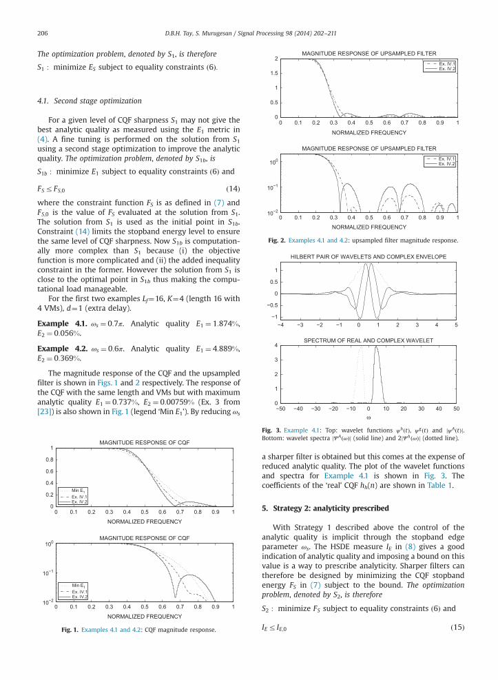
Fig. 2. Examples 4.1 and 4.2: upsampled filter magnitude response.

−4 −3 −2 −1 0 1 2 3 4 5−1

−0.5

0

0.5

1

HILBERT PAIR OF WAVELETS AND COMPLEX ENVELOPE

−50 −40 −30 −20 −10 0 10 20 30 40 500

1

2

3

4SPECTRUM OF REAL AND COMPLEX WAVELET


The optimization problem, denoted by S1, is therefore

S1 : minimize ES subject to equality constraints ð6Þ:

4.1. Second stage optimization

For a given level of CQF sharpness S1 may not give thebest analytic quality as measured using the E1 metric in(4). A fine tuning is performed on the solution from S1using a second stage optimization to improve the analyticquality. The optimization problem, denoted by S1b, is

S1b : minimize E1 subject to equality constraints ð6Þ and

FSrFS;0 ð14Þwhere the constraint function FS is as defined in (7) andFS;0 is the value of FS evaluated at the solution from S1.The solution from S1 is used as the initial point in S1b.Constraint (14) limits the stopband energy level to ensurethe same level of CQF sharpness. Now S1b is computation-ally more complex than S1 because (i) the objectivefunction is more complicated and (ii) the added inequalityconstraint in the former. However the solution from S1 isclose to the optimal point in S1b thus making the compu-tational load manageable.

For the first two examples Lf¼16, K¼4 (length 16 with4 VMs), d¼1 (extra delay).

Example 4.1. ωs ¼ 0:7π. Analytic quality E1 ¼ 1:874%,E2 ¼ 0:056%.

Example 4.2. ωs ¼ 0:6π. Analytic quality E1 ¼ 4:889%,E2 ¼ 0:369%.

The magnitude response of the CQF and the upsampledfilter is shown in Figs. 1 and 2 respectively. The response ofthe CQF with the same length and VMs but with maximumanalytic quality E1 ¼ 0:737%, E2 ¼ 0:00759% (Ex. 3 from[23]) is also shown in Fig. 1 (legend ‘Min E1’). By reducing ωs

0 0.1 0.2 0.3 0.4 0.5 0.6 0.7 0.8 0.9 10

0.2

0.4

0.6

0.8

1MAGNITUDE RESPONSE OF CQF


0 0.1 0.2 0.3 0.4 0.5 0.6 0.7 0.8 0.9 110−2

10−1



Fig. 1. Examples 4.1 and 4.2: CQF magnitude response.

ω

Fig. 3. Example 4.1: Top: wavelet functions ψhðtÞ, ψgðtÞ and jψAðtÞj.Bottom: wavelet spectra jΨAðωÞj (solid line) and 2jΨhðωÞj (dotted line).

a sharper filter is obtained but this comes at the expense ofreduced analytic quality. The plot of the wavelet functionsand spectra for Example 4.1 is shown in Fig. 3. Thecoefficients of the ‘real’ CQF hh(n) are shown in Table 1.

5. Strategy 2: analyticity prescribed

With Strategy 1 described above the control of theanalytic quality is implicit through the stopband edgeparameter ωs. The HSDE measure IE in (8) gives a goodindication of analytic quality and imposing a bound on thisvalue is a way to prescribe analyticity. Sharper filters cantherefore be designed by minimizing the CQF stopbandenergy FS in (7) subject to the bound. The optimizationproblem, denoted by S2, is therefore

S2 : minimize FS subject to equality constraints ð6Þ and

IEr IE;0 ð15Þ

Table 1CQF coefficients of Examples 4.1 and 4.2. Unity DC gain.

Example 4.1 Example 4.2

�0.009288070336952 �0.0192070286324000.002718354627698 0.0076125284661030.032614522408506 0.052365614789789

�0.037371473202580 �0.063096103175467�0.078757156755034 �0.0844985871923910.199938602548214 0.2258177755075200.535014188096851 0.5163576942663800.397894153009484 0.3985560465114690.010287049380210 0.021456201549304

�0.078795358386691 �0.0898092697340370.012248907060829 0.0174201231946700.015397682501713 0.019682335867207

�0.002332723487727 �0.004682242713824�0.000510708321440 �0.0007520685793450.000213283633295 0.0007882247372980.000728747223625 0.001988755137725

0 0.1 0.2 0.3 0.4 0.5 0.6 0.7 0.8 0.9 10

0.2

0.4

0.6

0.8



Ex. V.1Ex. V.2

0 0.1 0.2 0.3 0.4 0.5 0.6 0.7 0.8 0.9 110−2

10−1



Ex. V.1Ex. V.2

Fig. 4. Examples 5.1 and 5.2: CQF magnitude response.

Table 2CQF coefficients of Examples 5.1 and 5.2. Unity DC gain.


0.004403282465397 0.007961212072402�0.029551314898656 �0.062491822367854�0.071816109364812 �0.0779535951940370.183259484969296 0.2184015836285330.559445514703257 0.5452446025067320.380921511501596 0.375881673558980

�0.015812613190099 �0.018813419334972�0.038173000332859 �0.0373409601461540.023779925386250 0.0435611999498750.003543318760631 0.005549525326495


where IE;0 is the prescribed bound on the HSDE energy.Increasing IE;0 decreases the analytic quality but allows forsmaller FS, thus achieving a sharper CQF filter. Now theprescribed IE;0 value cannot be too small or else S2 isinfeasible. The smallest allowable value IE;min correspondsto the solution using the method in [23], where all degreesof freedom are used to minimize IE. The designer cantherefore use the IE;min value as a starting point andprogressively increase IE;0 above that value to get sharperfilters. The value of the stopband edge parameter ωs usedin FS is not important because the optimizer ability toreduce FS is limited by the constraint (15). The control ofthe trade-off between analytic quality and sharpness istherefore through the value IE;0 and not through ωs (whichis the case for S1). Compared to S1, S2 is computationallymore complex because of the inequality constraint (15).

Fine tuning of the solution using S1b described inSection 4.1 can be used to improve the analytic quality ofthe filter. FS;0 is now the value of FS evaluated at thesolution from S2, and the solution from S2 is now used asthe initial starting point. At this point it is fair to ask whynot use a constraint on the direct measure of analyticquality E1. As shown in [23] small IE implies small E1, andideally IE ¼ E1 ¼ 0, but the lowest IE value in general doesnot yield the lowest E1 value. However a constraint usingthe E1 measure instead of (15) would substantiallyincrease the computational load in S2. The philosophyhere is to use the E1 measure only in the fine tuning stagewhen a sub-optimal solution has already been found in thefirst stage.

For the next two examples Lf¼10, K¼2 (length 10 with2 VMs), d¼0 (extra delay). Now IE;min ¼ 8:18� 10�5. TheIE;0 value is now increased above IE;min.

Example 5.1. IE;0 ¼ 0:002. Analytic quality E1 ¼ 2:777%,E2 ¼ 0:138%.

Example 5.2. IE;0 ¼ 0:01. Analytic quality E1 ¼ 6:052%,E2 ¼ 0:741%.

The magnitude response of the CQFs is shown inFig. 4. The response of the CQF with the same length andVMs but with maximum analytic quality E1 ¼ 0:521%,

E2 ¼ 0:00820% (Ex. 1 from [23]) is also shown in Fig. 4(legend ‘Min E1’). Increasing IE;0 reduces the analyticquality but allows the optimizer to give sharper filters.The CQF coefficients are shown in Table 2.

6. Strategy 3: sharpness prescribed

In the examples above, using strategy 1 or 2, thefrequency response of the CQF H0ðejωÞ does not have zerosapart from those at ω¼ π. There appears however to be a‘pseudo-zero’ which looks like a ‘kink’ in the response,and is quite pronounced for Example 4.2 in Fig. 1. The‘kink’ occurs at a frequency ω′ where ReðH0ðejω′ÞÞ ¼ 0 andImðH0ðejω′ÞÞ is small but not strictly zero. However theequivalent upsampled filter has a strict zero at ω¼ ω′=2(half the ‘kink’ frequency), i.e. HSðejω′=2Þ ¼ 0. In general atthe corresponding aliased frequency ω¼ ðπ�ω′Þ=2, thealiasing HSðejðπ�ω′Þ=2Þa0, but is usually small and contri-butes to a non-zero ‘kink’.

For a strict zero at frequency ω¼ω0 both the real andimaginary parts of H0ðejωÞ need to be simultaneously zeroat ω¼ω0. Using (10) it can be readily shown that this isequivalent to having zeros at frequencies ω¼ ω0=2 andω¼ ðπ�ω0Þ=2 for the upsampled filter. Having strict zerosin the stopband is typical for most sharp low-pass filters

0 0.1 0.2 0.3 0.4 0.5 0.6 0.7 0.8 0.9 10

0.2

0.4

0.6

0.8



No pinsSpeech opt.Ex. VI.1

0 0.1 0.2 0.3 0.4 0.5 0.6 0.7 0.8 0.9 110−3

10−2

10−1



No pinsSpeech opt.Ex. VI.1

Fig. 5. Example 6.1: CQF magnitude response.

0.2

0.4

0.6

0.8


No pinsEx. VI.2


and is an effective mechanism for achieving sharp cut-offfilters. Therefore the strategy here is to impose zeros onthe un-normalized CQF at the stopband frequenciesω0;ω1;…;ωP:

ReðH0ðejωl ÞÞ ¼ ∑L

n ¼ �ðL�1Þh0ðnÞ cos ωl ¼ 0 ð16Þ

ImðH0ðejωl ÞÞ ¼ ∑L

n ¼ �ðL�1Þh0ðnÞ sin ωl ¼ 0 ð17Þ

for l¼ 1;…; P. Since h0ðnÞ is multilinear in the latticeparameters αl, Eqs. (16) and (17) have a similar form tothat shown in (6). The principle of prescribing zeros wasproposed previously in [25] for single filter bank andextended in [22] for SSH filters. However in [25,22] thezeros were imposed on the product filter, resulting inlinear constraints on the Bernstein polynomial parameters,but here the zero is imposed directly on the CQF. With theproduct filter a double zero is needed to ensure non-negativity of its real-valued frequency response [25,22].Although the final effect is the same the constraint equa-tions resulting from the two approaches are quite differentmathematically. Each imposed zero uses up two degrees offreedom, and can be considered as the result of reducingthe number of VMs by two, or moving a pair of zeros fromz¼ �1 along the unit circle to z¼ e7 jωl .

Just like with previous strategies a two stage approachis adopted here:

0 0.1 0.2 0.3 0.4 0.5 0.6 0.7 0.8 0.9 10

1.

Optimization problem S3:S3 : minimize IE subject to equalityconstraints (6), (16) and (17).

2.

10−2

10−1

No pins

Fine tuning optimization S3b:S3b : minimize E1 subject to equalityconstraints (6), (16) and (17).

using the solution from S3 as the initial point.

0 0.1 0.2 0.3 0.4 0.5 0.6 0.7 0.8 0.9 110−3


Ex. VI.2

Fig. 6. Example 6.2: CQF magnitude response.

With the approach proposed here one can prescribeexactly the number of degrees of freedom for each of thethree competing criteria: (i) number of VMs K, (ii) sharp-ness via number of pinned zeros P, and (iii) analytic qualitynf ¼ Lf =2�K�2P. Shaping of the stopband is easily doneusing the pinned zeros. When the number of zeros P issmall (as with the examples here) simple rules asdescribed in [25] can be used. Alternatively one can usethe zeros from existing CQF, such as in [30], and thenreduce the number of VMs to address the analytic qualitycriterion.

Consider now the CQF from Example 3 in [30] which isof length 12, with 4 VMs, and has been optimized withrespect to a speech signal. That CQF can be obtained bypinning a zero at ω0 ¼ 0:713π which requires two degreesof freedom. The remaining 4 degrees are for VMs. In thenext example reducing the VMs by two allows nf¼2 foranalytic quality.

Example 6.1. Lf¼12, d¼1, K¼2, P¼1 and ω0 ¼ 0:713π, thesame as in Ex. 3 in [30]. The magnitude response of theCQF is shown in Fig. 5 and is quite similar to the response

in [30] (legend ‘Speech Opt.’ in figure). The analytic qualityhere is E1 ¼ 3:644%, E2 ¼ 0:100% compared toE1 ¼ 37:54%, E2 ¼ 15:26% in [30], and the latter was notdesigned with analyticity in mind. The pinned zero can beconsidered as the result of reducing the number of VMs by2. For further comparison consider the CQF with 4 VMs,nf¼2 for analytic quality, designed using the method in[23]. The response is less sharp in comparison (legend ‘Nopins’ in same figure) but the analytic quality E1 ¼ 3:420%,E2 ¼ 0:241% is comparable. Sharpness is achieved here atthe expense of reduced VMs.

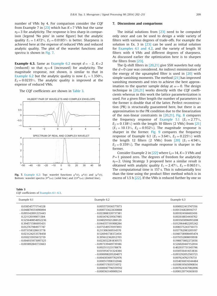
Example 6.2. Lf¼20, d¼1, K¼3, P¼2 and ðω0;ω1Þ ¼ð0:7π;0:8πÞ. Now nf¼3 for analyticity. The magnituderesponse of the CQF is shown in Fig. 6 and the analyticquality is E1 ¼ 3:043%, E2 ¼ 0:0755%. The two pinnedzeros can be considered as the result of reducing the


number of VMs by 4. For comparison consider the CQFfrom Example 7 in [23] which has K¼7 VMs but the samenf¼3 for analyticity. The response is less sharp in compar-ison (legend ‘No pins’ in same figure) but the analyticquality E1 ¼ 1:472%, E2 ¼ 0:0185% is better. Sharpness isachieved here at the expense of reduced VMs and reducedanalytic quality. The plot of the wavelet functions andspectra is shown in Fig. 7.

Example 6.3. Same as Example 6.2 except d¼ �2, K¼2(reduced) so that nf¼4 (increased) for analyticity. Themagnitude response, not shown, is similar to that inExample 6.2 but the analytic quality is now E1 ¼ 1:350%,E2 ¼ 0:0235%. The analytic quality is improved at theexpense of reduced VMs.

The CQF coefficients are shown in Table 3.

−4 −2 0 2 4 6−1

−0.5

0

0.5

1

HILBERT PAIR OF WAVELETS AND COMPLEX ENVELOPE

−50 −40 −30 −20 −10 0 10 20 30 40 500

1

2

3

4SPECTRUM OF REAL AND COMPLEX WAVELET

ω

Fig. 7. Example 6.2: Top: wavelet functions ψhðtÞ, ψgðtÞ and jψAðtÞj.Bottom: wavelet spectra jΨAðωÞj (solid line) and 2jΨhðωÞj (dotted line).

Table 3CQF coefficients of Examples 6.1–6.3.


0.038545771714328 0.005573936�0.048874551090094 0.00073362�0.095142891225443 �0.0228883200.221120199071384 0.0034742390.525640854052236 0.0402919210.394571586693431 �0.0443571910.012767984977747 �0.075549570

�0.073158328613778 0.2113063690.023124253578458 0.5269417380.010233935672719 0.395612362

�0.004935973097325 0.022652281�0.003892841733663 �0.097339449

0.0025113230.035954731

�0.00009820�0.004303690.000517098

�0.0007178350.00004779

�0.000363149

7. Discussions and comparisons

The initial solutions from [23] need to be computedonly once and can be used to design a wide variety offilters with various degrees of trade-offs. For example thesolution in Ex. 3 in [23] can be used as initial solutionfor Examples 4.1 and 4.2, and the variety of length 16filters with 4 VMs and different degrees of sharpness.As discussed earlier the optimization here is to sharpenthe filters from [23].

The Q-shift filters in [20,21] give SSH wavelets but onlythe d¼0 case was considered. An indirect minimization ofthe energy of the upsampled filter is used in [20] withsimple vanishing moments. The method [21] has improvedvanishing moments and tries to achieve the best approx-imation to the quarter sample delay at ω¼ 0. The designtechnique in [20,21] works directly with the CQF coeffi-cients whereas in this work the lattice parameterization isused. For a given filter length the number of parameters inthe former is double that of the latter. Perfect reconstruc-tion (PR) is structurally guaranteed here, but there is anapproximation to the PR condition due to the linearizationof the non-linear constraints in [20,21]. Fig. 8 comparesthe frequency response of Example 5.1 (E1 ¼ 2:77%,E2 ¼ 0:138%) with the length 10 filters (2 VMs) from [21](E1 ¼ 10:13%, E2 ¼ 0:932%). The magnitude response issharper in the former. Fig. 9 compares the frequencyresponse of Example 6.1 (E1 ¼ 3:64%, E2 ¼ 0:225%) withthe length 12 filters (2 VMs) from [20] (E1 ¼ 4:94%,E2 ¼ 0:359%). The magnitude response is sharper in theformer.

Consider Example 2 in [22] where Lf¼14, K¼3 VMs andP¼1 pinned zero. The degrees of freedom for analyticitynf¼2. Using Strategy 3 proposed here a similar result isobtained with analytic quality E1 ¼ 2:47%, E2 ¼ 0:0651%.The computational time is 157 s. This is substantially lessthan the time using the product filter method which is inexcess of 1.5 h [22]. If the VMs is reduced further by one so

Example 6.3

577873 0.0000224137473562630888 �0.001316828916717737381 0.001924166602416567985 0.002618834410762288129 0.003503096093208908284 �0.012964462205242197893 0.008375243756173514570 0.037762983205197372454 �0.048758908495474012703 �0.079352808019918830575 0.198875802272656739186 0.526020447152014178879 0.402937731345796324384 0.0305564116538365204071 �0.0932920525837217762976 0.007624762176731332046 0.034036874344484731072 �0.0108195650908546559592 �0.007624367082896909214 �0.000129774365810

0 0.1 0.2 0.3 0.4 0.5 0.6 0.7 0.8 0.9 10

0.2

0.4

0.6

0.8



Ex. V.1Ref. [24]

0 0.1 0.2 0.3 0.4 0.5 0.6 0.7 0.8 0.9 110−2

10−1



Ex. V.1Ref. [24]

Fig. 8. Comparison of length 10 CQF from Example 5.1 and from [21].

0 0.1 0.2 0.3 0.4 0.5 0.6 0.7 0.8 0.9 10

0.2

0.4

0.6

0.8



Ex. VI.1Ref. [23]

0 0.1 0.2 0.3 0.4 0.5 0.6 0.7 0.8 0.9 110−2

10−1



Ex. VI.1Ref. [23]

Fig. 9. Comparison of length 12 CQF from Example 6.1 and from [20].


that nf¼3, the improved analytic quality is E1 ¼ 1:38%,E2 ¼ 0:0333%. The computational time is now 125 s. Withthe product filter method [22] the computational time willsubstantially increase beyond 1.5 h and is not practical.The time is proportional to the number of search pointwhich is Nnf

G , where NG is the number of discrete points perdimension, and is usually several hundreds. Strategy 3 alsogives a similar result to Example 4 in [22] where Lf¼18,K¼3 VMs, P¼2 pinned zeros, nf¼2 with analytic qualityE1 ¼ 3:88%, E2 ¼ 0:096%. If the VMs is reduced further byone so that nf¼3, the improved analytic quality is thenE1 ¼ 2:48%, E2 ¼ 0:054%.

8. Conclusions

A suite of three algorithms has been presented for thedesign of SSH wavelet filters with sharper frequency

response. The algorithms are based on optimizing theorthogonal lattice parameters. The algorithms easily allowthe trade-off between the competing criteria of degree ofsharpness and analytic quality. The algorithms work withany degrees of freedom and are substantially more effi-cient than the method based on the product filter, which isonly practical with small degrees of freedom. The suiteof algorithms allows a wide variety of filters to be tailoredto the designers specification, and this has been demon-strated with the design examples.

References

[1] S. Issac, P. Palanisamy, K. Sujathan, E. Bengtsson, Analysis of nucleitextures of fine needle aspirated cytology images for breast cancerdiagnosis using Complex Daubechies wavelets, Signal Process. 93(October (10)) (2013) 2828–2837.

[2] S.T.N. Nguyen, B.W.-H. Ng, Bi-orthogonal rational discrete wavelettransform with multiple regularity orders and application experi-ments, Signal Process. 93 (November (11)) (2013) 3014–3026.

[3] X. Zhang, X. Wang, Chaos-based partial encryption of SPIHT codedcolor images, Signal Process. 93 (September (9)) (2013) 2422–2431.

[4] R. Rubinstein, A.M. Bruckstein, M. Elad, Dictionaries for sparse repre-sentation modeling, Proc. IEEE 98 (June (6)) (2010) 1045–1057.

[5] Y. Qin, J. Wang, B. Tang, Y. Mao, Higher density wavelet frames withsymmetric low-pass and band-pass filters, Signal Process. 90(December (12)) (2010) 3219–3231.

[6] I.W. Selesnick, R.G. Baraniuk, N.G. Kingsbury, The dual-tree complexwavelet transform, IEEE Signal Process. Mag. 22 (November (6))(2005) 123–151.

[7] S. Yin, L. Cao, Y. Ling, G. Jin, Image denoising with anisotropic bivariateshrinkage, Signal Process. 91 (August (8)) (2011) 2078–2090.

[8] A. Vo, S. Oraintara, N. Nguyen, Vonn distribution of relative phase forstatistical image modeling in complex wavelet domain, SignalProcess. 91 (January (1)) (2011) 114–125.

[9] D.B.H. Tay, Designing Hilbert-pair of wavelets: recent progress andfuture trends, in: International Conference on Information, Commu-nications and Signal Processing ICICS 2007, Singapore, December 2007.

[10] B. Dumitrescu, I. Bayram, I.W. Selesnick, Optimization of symmetricself-Hilbertian filters for the dual-tree filter complex wavelet trans-form, IEEE Signal Proc. Lett. 15 (2008) 146–149.

[11] H. Shi, B. Hu, J.-Q. Zhang, A novel scheme for the design ofapproximate Hilbert transform pairs of orthonormal wavelet bases,IEEE Trans. Signal Process. 56 (June (6)) (2008) 2289–2297.

[12] B. Dumitrescu, SDP approximation of a fractional delay and thedesign of dual-tree filter complex wavelet transform, IEEE Trans.Signal Process. 56 (September (9)) (2008) 4255–4262.

[13] J. Wang, J.-Q. Zhang, A globally optimal bilinear programming approachto the design of approximate Hilbert pairs of orthonormal waveletbases, IEEE Trans. Signal Process. 58 (January (1)) (2010) 233–241.

[14] D.B.H. Tay, A new approach to the common-factor design techniquefor Hilbert-pair of wavelets, IEEE Signal Process. Lett. 17 (November(11)) (2010) 969–972.

[15] X. Zhang, A new phase-factor design method for Hilbert-pairs oforthonormal wavelets, IEEE Signal Process. Lett. 18 (September (9))(2011) 529–532.

[16] S. Murugesan, D.B. Tay, A new class of almost symmetric orthogonalHilbert pair of wavelets, Signal Process. 95 (February) (2014) 76–87.

[17] D.B.H. Tay, N.G. Kingsbury, M. Palaniswami, Orthonormal Hilbertpair of wavelets with (Almost) maximum vanishing moments, IEEESignal Process. Lett. 13 (September (19)) (2006) 533–536.

[18] N. Kingsbury, A dual-tree complex wavelet transformwith improvedorthogonality and symmetry properties, in: Proceedings of the IEEEInternational Conference on Image Processing (ICIP), vol. 2, Septem-ber 2000, pp. 375–378.

[19] N. Kingsbury, Complex wavelets for shift invariant analysis andfiltering of signals, J. Appl. Comput. Harmonic Anal. 10 (May (3))(2001) 234–253.

[20] N. Kingsbury, Design of Q-shift complex wavelets for image proces-sing using frequency domain energy minimization, in: Proceedingsof the IEEE International Conference on Image Processing (ICIP), vol.1, September 2003, pp. 1013–1016.

[21] X. Zhang, Design of Q-shift filters with improved vanishing momentsfor DTCWT, in: Proceedings of the IEEE International Conference onImage Processing (ICIP), September 2011, pp. 257–260.

http://refhub.elsevier.com/S0165-1684(13)00476-3/sbref1

















































[22] D.B.H. Tay, Symmetric self-Hilbertian filters via extended zero-pinning, Signal Process. 92 (February (2)) (2012) 392–400.

[23] D.B.H. Tay, Symmetric self-Hilbertian wavelets via orthogonal latticeoptimization, IEEE Signal Process. Lett. 19 (July (7)) (2012) 387–390.

[24] P.P. Vaidyanathan, Multirate Systems and Filter Banks, Prentice-Hall,1993.

[25] D.B.H. Tay, Zero-pinning the Bernstein Polynomial: a simple designtechnique for orthonormal wavelets, IEEE Signal Process. Lett. 12(December (12)) (2005) 835–838.

[26] I.W. Selesnick, Hilbert transform pairs of wavelet bases, IEEE SignalProcess. Lett. 8 (June (6)) (2001) 170–173.

[27] C. Chaux, L. Duval, J.-C. Pesquet, Image analysis using a dual-treeM-band wavelet transform, IEEE Trans. Image Process. 15 (August(8)) (2006) 2397–2412.

[28] D.B.H. Tay, Hilbert pair of orthogonal wavelet bases: revisiting thecondition, IEEE Trans. Signal Process. 56 (April (4)) (2008) 1716–1721.

[29] R.A. Waltz, J.L. Morales, J. Nocedal, D. Orban, An interior algorithmfor nonlinear optimization that combines line search and trustregion steps, Math. Program. 107 (3) (2006) 391–408.

[30] J.-K. Zhang, T. Davidson, K.M. Wong, Efficient design of orthonormalwavelet bases for signal representation, IEEE Trans. Signal Process.52 (July (7)) (2004) 1983–1996.























sharper symmetric self-hilbertian wavelets

Documents