sharp inequalities in harmonic analysis · sharp inequalities in harmonic analysis summer school,...
TRANSCRIPT

Sharp Inequalities in Harmonic Analysis
Summer School∗, Kopp
August 30th - September 4th, 2015
Organizers:
Rupert FrankCalifornia Institute of Technology, Pasadena, USA
Diogo Oliveira e SilvaUniversity of Bonn, Germany
Christoph ThieleUniversity of Bonn, Germany
∗supported by Hausdorff Center for Mathematics, Bonn

Contents
1 Maximizers for the Strichartz inequality 5David Beltran, University of Birmingham . . . . . . . . . . . . . . . 51.1 Introduction . . . . . . . . . . . . . . . . . . . . . . . . . . . . 51.2 Connection to Fourier restriction theorems . . . . . . . . . . . 61.3 Scheme of the proof . . . . . . . . . . . . . . . . . . . . . . . . 8
1.3.1 Case of general wave equation . . . . . . . . . . . . . . 10
2 A sharpened Hausdorff-Young inequality 11Amalia Culiuc, Brown University . . . . . . . . . . . . . . . . . . . 112.1 Introduction . . . . . . . . . . . . . . . . . . . . . . . . . . . . 112.2 Main results . . . . . . . . . . . . . . . . . . . . . . . . . . . . 122.3 Proof of Proposition 3 . . . . . . . . . . . . . . . . . . . . . . 13
3 A note on the Sobolev inequality 16Alexis Drouot, University of California, Berkeley . . . . . . . . . . . 163.1 Introduction . . . . . . . . . . . . . . . . . . . . . . . . . . . . 163.2 Symmetries of the inequality . . . . . . . . . . . . . . . . . . . 173.3 Local version of theorem 2 . . . . . . . . . . . . . . . . . . . . 183.4 Proof of theorem 2 and comments. . . . . . . . . . . . . . . . 20
4 Gaussian kernels have only Gaussian maximizers 22Polona Durcik, University of Bonn . . . . . . . . . . . . . . . . . . 224.1 Introduction . . . . . . . . . . . . . . . . . . . . . . . . . . . . 224.2 Non-degenerate Gaussian kernels . . . . . . . . . . . . . . . . 24
4.2.1 Sketch of proofs . . . . . . . . . . . . . . . . . . . . . . 254.3 Degenerate Gaussian kernels . . . . . . . . . . . . . . . . . . . 264.4 Closing remarks . . . . . . . . . . . . . . . . . . . . . . . . . . 27
5 A New, Rearrangement-free Proof of the SharpHardy-Littlewood-Sobolev Inequality 28Taryn C Flock, University of Birmingham . . . . . . . . . . . . . . 285.1 Introduction . . . . . . . . . . . . . . . . . . . . . . . . . . . . 28
5.1.1 The Hardy-Littlewood-Sobolev Inequality . . . . . . . 285.1.2 Outline of Proof . . . . . . . . . . . . . . . . . . . . . 29
5.2 Sketch of Proof . . . . . . . . . . . . . . . . . . . . . . . . . . 305.2.1 Existence of Extremizers . . . . . . . . . . . . . . . . . 30
1

5.2.2 Uplifting the problem . . . . . . . . . . . . . . . . . . . 305.2.3 Vanishing center of mass . . . . . . . . . . . . . . . . . 305.2.4 Two Inequalities . . . . . . . . . . . . . . . . . . . . . 30
6 Maximizers for the adjoint Fourier restriction inequality onthe sphere 33Marius Lemm, California Institute of Technology (Caltech), Pasadena 336.1 Introduction and main result . . . . . . . . . . . . . . . . . . . 336.2 Sketch of the proof . . . . . . . . . . . . . . . . . . . . . . . . 34
7 Extremals of functionals with competing symmetries 39Teresa Luque, ICMAT - Instituto de Ciencias Matematicas, Madrid 397.1 Introduction . . . . . . . . . . . . . . . . . . . . . . . . . . . . 397.2 The competing transformations . . . . . . . . . . . . . . . . . 417.3 Competing symmetries . . . . . . . . . . . . . . . . . . . . . . 427.4 Applications . . . . . . . . . . . . . . . . . . . . . . . . . . . . 43
7.4.1 The Hardy-Littlewood Sobolev inequality . . . . . . . . 437.4.2 The logarithmic Sobolev inequality . . . . . . . . . . . 44
8 Extremals for the Tomas-Stein inequality 45Dominique Maldague, University of California, Berkeley . . . . . . 458.1 Introduction . . . . . . . . . . . . . . . . . . . . . . . . . . . . 458.2 Two Principles . . . . . . . . . . . . . . . . . . . . . . . . . . 468.3 Sufficient properties for extremizing sequences . . . . . . . . . 47
8.3.1 Nonnegativity . . . . . . . . . . . . . . . . . . . . . . . 478.3.2 Symmetrization . . . . . . . . . . . . . . . . . . . . . . 47
8.4 Technical tools: Caps and gauge functions . . . . . . . . . . . 488.5 Almost upper even-normalization . . . . . . . . . . . . . . . . 498.6 Resulting concentration . . . . . . . . . . . . . . . . . . . . . . 49
8.6.1 Ruling out concentration to a δ-function . . . . . . . . 50
9 Heat-flow monotonicity of Strichartz norms 53Lisa Onkes, University of Bonn . . . . . . . . . . . . . . . . . . . . 539.1 Introduction: Strichartz estimates for the free
Schrodinger equation . . . . . . . . . . . . . . . . . . . . . . . 539.2 The heat-flow monotonicity property . . . . . . . . . . . . . . 54
9.2.1 Proof sketch of the monotonicity property . . . . . . . 559.3 Higher dimensions . . . . . . . . . . . . . . . . . . . . . . . . 57
2

10 Multidimensional van der Corpus and sublevel set estimates 59Guillermo Rey, Michigan State University . . . . . . . . . . . . . . 5910.1 Introduction . . . . . . . . . . . . . . . . . . . . . . . . . . . . 5910.2 The one-dimensional case . . . . . . . . . . . . . . . . . . . . . 5910.3 Higher dimensions . . . . . . . . . . . . . . . . . . . . . . . . 61
10.3.1 The two-dimensional case . . . . . . . . . . . . . . . . 6110.4 Applications and further remarks . . . . . . . . . . . . . . . . 63
11 Optimal Young’s inequality and its converse: a simple proof 65Johanna Richter, University of Stuttgart . . . . . . . . . . . . . . . 6511.1 Introduction and main result . . . . . . . . . . . . . . . . . . . 6511.2 Reformulation of the problem . . . . . . . . . . . . . . . . . . 6611.3 The key element of the proof . . . . . . . . . . . . . . . . . . . 6711.4 Proof of Theorem 2 . . . . . . . . . . . . . . . . . . . . . . . . 6811.5 Extremizers . . . . . . . . . . . . . . . . . . . . . . . . . . . . 69
12 Extremizers of a Radon transform inequality 71Joris Roos, University of Bonn . . . . . . . . . . . . . . . . . . . . . 7112.1 Introduction . . . . . . . . . . . . . . . . . . . . . . . . . . . . 7112.2 Some ingredients of the proof . . . . . . . . . . . . . . . . . . 73
12.2.1 Connection of R,R], C. . . . . . . . . . . . . . . . . . . 7312.2.2 Affine invariance. . . . . . . . . . . . . . . . . . . . . . 7312.2.3 An additional symmetry. . . . . . . . . . . . . . . . . . 7412.2.4 Drury’s identity. . . . . . . . . . . . . . . . . . . . . . . 7412.2.5 A rearrangement inequality. . . . . . . . . . . . . . . . 7512.2.6 Burchard’s theorem. . . . . . . . . . . . . . . . . . . . 75
13 Existence of extremizers for a family of extension operators 77Julien Sabin, Universite Paris-Sud, Orsay . . . . . . . . . . . . . . . 7713.1 Introduction . . . . . . . . . . . . . . . . . . . . . . . . . . . . 7713.2 An abstract result on the existence of extremizers . . . . . . . 7813.3 Application to extension operators in the finite volume setting 7913.4 An application in infinite volume: Strichartz estimates . . . . 82
14 The Sharp Hausdorff-Young Inequality 86Mateus Sousa, IMPA - Instituto Nacional de Mathematica Pura e
Aplicada, Rio de Janeiro . . . . . . . . . . . . . . . . . . . . . 8614.1 Introduction . . . . . . . . . . . . . . . . . . . . . . . . . . . . 86
3

14.2 Discrete analogue of Tω . . . . . . . . . . . . . . . . . . . . . . 8714.3 Bounds for the discrete analogue . . . . . . . . . . . . . . . . 8914.4 Hermite polynomials, symmetric functions and the result . . . 89
15 A mass-transportation approach to sharp Sobolev andGagliardo-Nirenberg inequalities 92Gennady Uraltsev, University of Bonn . . . . . . . . . . . . . . . . 9215.1 Introduction and generalities . . . . . . . . . . . . . . . . . . . 92
15.1.1 Norms and Geometry of Rn . . . . . . . . . . . . . . . 9315.1.2 Scaling and duality . . . . . . . . . . . . . . . . . . . . 93
15.2 The main result . . . . . . . . . . . . . . . . . . . . . . . . . . 9315.3 Some notions about mass transport and convex functions . . . 9415.4 Sketch of the proof . . . . . . . . . . . . . . . . . . . . . . . . 9615.5 Remarks and further topics . . . . . . . . . . . . . . . . . . . 96
16 Brunn-Minkowski inequalities and log concave functions 98Michal Warchalski, University of Bonn . . . . . . . . . . . . . . . . 9816.1 Introduction . . . . . . . . . . . . . . . . . . . . . . . . . . . . 9816.2 Application - the isoperimetric inequality . . . . . . . . . . . . 9916.3 The first proof . . . . . . . . . . . . . . . . . . . . . . . . . . . 10116.4 The second proof . . . . . . . . . . . . . . . . . . . . . . . . . 102
17 Sharp fractional Hardy inequalities 104An Zhang, Peking University, CH / University of Paris, FR . . . . . 10417.1 Introduction . . . . . . . . . . . . . . . . . . . . . . . . . . . . 10417.2 A general setting and examples . . . . . . . . . . . . . . . . . 106
17.2.1 General setting . . . . . . . . . . . . . . . . . . . . . . 10617.2.2 Examples . . . . . . . . . . . . . . . . . . . . . . . . . 106
17.3 Proof of the theorem . . . . . . . . . . . . . . . . . . . . . . . 107
18 Optimal Young inequality: a symmetric proof 110Pavel Zorin-Kranich, University of Bonn . . . . . . . . . . . . . . . 110
4

1 Maximizers for the Strichartz inequality
after D. Foschi [2]A summary written by David Beltran
Abstract
We give the sharp constant and a characterisation of the maximis-ers for the Strichartz estimates for the homogeneous free Schrodingerequation (for dimensions d = 1, 2) and the homogeneous wave equation(for dimension d = 3). In the context of Fourier restriction estimates,we obtain the sharp constant and maximisers for the Stein-Tomastheorem in the paraboloid (d = 1, 2) and in the cone (d = 2, 3).
1.1 Introduction
Consider the homogeneous free Schrodinger equation,
i∂tu−∆u = 0, u(0, x) = u0(x), (1)
where (t, x) ∈ R1+d. Strichartz [3] showed that there exists a constant S suchthat
‖u‖Lp(Rd+1) ≤ S‖u0‖L2(Rd), p = 2 + 4/d. (2)
For d ≥ 2, he also established a similar kind of estimate for the solutionof the homogeneous wave equation, that is, if u satisfies
∂2ttu−∆u = 0, u(0, x) = u0(x), ∂tu(0, x) = u1(x), (3)
then there exists a constant W such that
‖u‖Lp(R1+d) ≤ W‖(u0, u1)‖H
12 (Rd)×H−
12 (Rd)
, p =2(d+ 1)
d− 1, (4)
where
‖(u0, u1)‖H
12 (Rd)×H−
12 (Rd)
=(‖u0‖2
H12 (Rd)
+ ‖u1‖2
H−12 (Rd)
)1/2
and Hs denotes the homogeneous Sobolev space, with ‖f‖Hs = ‖(−∆)s2f‖L2 .
Let S(d) and W (d) denote the best constant in (2) and (4) respectively.The main result of the article under review is to provide the values of S(1),S(2) and W (3) and to characterise the set of extremisers in such cases.
In the case of the Schrodinger equation we have the following.
5

Theorem 1. For (d, p) = (1, 6) we have S(1) = 12−1/12. For (d, p) = (2, 4)we have S(2) = 2−1/2. Given the initial data u∗0(x) = e−|x|
2, let u∗(t, x)
be the corresponding solution to the Schrodinger equation. Then for bothd = 1, 2 the set of extremisers for (2) is given by the initial data of solutionsto (1) in the orbit of u∗ under the action of the group of symmetries for theSchrodinger equation. In particular, they are given by L2(Rd) functions ofthe form
u0(x) = eA|x|2+b·x+C ,
with A,C ∈ C, b ∈ Cd and <(A) < 0.
In the case of the wave equation we have
Theorem 2. Let (d, p) = (3, 4). Then W (3) = (3/(16π))1/4. Given theinitial data u∗0(x) = (1 + |x|2)−(d−1)/2, u∗1(x) = 0, let u∗ be the correspondingsolution to the wave equation. Then the set of extremisers for (4) is the setof initial data of the solutions to (3) in the orbit of u∗ under the action ofthe group of symmetries for the wave equation.
Remark 3. In [2] it is also stated a similar result to Theorem 2 when d = 2,but Foschi’s argument turned out to be incorrect, as remarked in [1]. How-ever, the result remains true for the wave propagator, and thus for Stein-Tomas Fourier restriction estimate in the cone - see the forthcoming section.
1.2 Connection to Fourier restriction theorems
The Strichartz estimates for the Schrodinger and wave equation are closelyrelated to Fourier restriction estimates. In the case of the Schrodinger equa-tion, the solution u is given by
u(t, x) = e−it∆u0(x) =
ˆRdu0(ξ)ei(t|ξ|
2+x·ξ)dξ,
where denotes the spatial Fourier transform 1. Taking space-time – (d+1)-dimensional – Fourier transform
u(τ, ξ) = 2πu0(ξ)δ(τ − |ξ|2),
1The definition we take of the Fourier transform along this review is f(ξ) =´Rd f(x)e−ix·ξdx. With this normalisation fg(ξ) = (2π)−df ∗ g(ξ) and ‖f‖L2(Rd) =
(2π)d/2‖f‖L2(Rd).
6

so u is supported in the paraboloid (τ, ξ) ∈ R1+d : τ = |ξ|2. Thus we may
write u as vdσ, where dσ is the induced Lebesgue measure on the paraboloidand v is the lift of u0 onto the paraboloid. The Strichartz estimate (2) isthen equivalent to the Fourier restriction estimate
‖vdσ‖L
2(d+2)d (Rd+1)
≤ (2π)−d/2S‖v‖L2(dσ),
which is the Stein-Tomas [4] Fourier restriction estimate for the paraboloid2.Hence, Theorem 1 gives sharp constant and extremisers for Stein-Tomas inthe paraboloid when d = 1, 2.
Similarly, one may link the solution to the wave equation with the re-striction of the Fourier transform to a cone. A solution u to (3) satisfies
u(t, ξ) = u0(ξ) cos(t|ξ|) +u1(ξ)
|ξ|sin(t|ξ|),
and it may be written as u = u+ + u−, with
u±(t) = e±it√−∆(√−∆)−
12f±, f± =
1
2
((√−∆)
12u0 ∓ i(
√−∆)−
12u1
).
Here
eit√−∆f(x) =
ˆRdf(ξ)ei(t|ξ|+x·ξ)dξ,
which is typically referred to as the one-sided wave propagator. Taking space-time Fourier transform,
u±(τ, ξ) = 2π|ξ|−12 δ(τ ∓ |ξ|)f±(ξ)
and one may write u+(−t,−x) = vdσ(t, x), where dσ is the induced Lebesgue
measure in the cone and v(|ξ|, ξ)|ξ|− 12 = f+(ξ); similarly for u−. Thus, the
estimate‖u+‖
L2(d+1)d−1 (Rd+1)
≤ C‖f+‖L2(Rd) (5)
is equivalent to
‖vdσ‖L
2(d+1)d−1 (Rd+1)
≤ (2π)−d/2C‖v‖L2(dσ),
which is the Stein-Tomas Fourier restriction estimate in the cone. Sharpconstant and characterisation of extremisers for the estimates (5) in the cased = 2, 3 are established in the article under review, so one obtains the anal-ogous result for Stein-Tomas in the cone.
2Of course the constant in the restriction estimate depends on the normalisation of theFourier transform.
7

1.3 Scheme of the proof
We first sketch the proof of Theorem 1 and the estimates (5), which all followthe same structure. Observe that by Plancherel’s theorem,
‖u‖p/2Lp(Rd+1)
= ‖up/2‖L2(Rd+1) = (2π)−(d+1)/2‖up/2‖L2(Rd+1),
and if p is an even integer, we may write up/2 as the convolution of u withitself p/2 times.
The method presented strongly relies on the fact p is an even integer, so itmay only provide results for d = 1, 2 in the case of the Schrodinger equation(recall that p = 2 + 4/d) and for d = 2, 3 in the case of the wave propagator(here p = 2(d+ 1)/(d− 1)).
Consider the Schrodinger case for d = 1. Observe that
u3(τ, ξ) =1
2π
ˆR×R×R
u0(η1)u0(η2)u0(η3)δ
(τ − η2
1 − η22 − η2
3
ξ − η1 − η2 − η3
)dη.
Then u3 is supported in the closure of the region
P1 = (τ, ξ) ∈ R× R : 3τ > ξ2.
For each (τ, ξ) ∈ P1, we define 〈·, ·〉(τ,ξ) to be the L2 inner product associatedwith the measure
µ(τ,ξ) = δ
(τ − η2
1 − η22 − η2
3
ξ − η1 − η2 − η3
)dη,
and let ‖ · ‖(τ,ξ) be the associated norm. Then one may write
u3(τ, ξ) =1
2π〈u0 ⊗ u0 ⊗ u0, 1⊗ 1⊗ 1〉(τ,ξ).
The Cauchy-Schwarz’s inequality gives
|u3(τ, ξ)| ≤ 1
2π‖u0 ⊗ u0 ⊗ u0‖(τ,ξ)‖1⊗ 1⊗ 1‖(τ,ξ).
For each (τ, ξ) ∈ P1, ‖1⊗ 1⊗ 1‖(τ,ξ) = (π/√
3)1/2. Also,
ˆP1
‖u0 ⊗ u0 ⊗ u0‖2(τ,ξ)dτdξ =
ˆR3
|3∏j=1
u0(ηj)|2ˆP1
µ(τ,ξ)dτdξ
= ‖u0 ⊗ u0 ⊗ u0‖2L2(R3) = (2π)3‖u0‖6
L2(R).
8

So, putting all together,
‖u‖L6(R2) ≤ 12−1/12‖u0‖L2(R),
with equality if there is equality in the application of the Cauchy-Schwarzinequality. That is, if there exists a scalar function F : P1 → C such that
(u0 ⊗ u0 ⊗ u0)(η) = F (τ, ξ)(1⊗ 1⊗ 1)(η)
for almost all η in the support of the measure µ(τ,ξ). Thus, we need functionsu0 and F such that
u0(η1)u0(η2)u0(η3) = F (η21 + η2
2 + η23, η1 + η2 + η3). (6)
Examples of functions satisfying the above equality are given by u0(ξ) = e−ξ2
and F (τ, ξ) = e−τ .The proofs for the Schrodinger case when d = 2 and the wave propagator
when d = 2, 3 follow the same pattern; the major changes are
• Schrodinger (d = 2). Measure µ(τ,ξ) = δ(τ−|η|2−|ζ|2ξ−η−ζ
)dηdζ, ‖1⊗ 1‖(τ,ξ) =√
π/2, and equality if u0 and F are such that
u0(η)u0(ζ) = F (|η|2 + |ζ|2, η + ζ). (7)
• Wave propagator (d = 2). Measure µ(τ,ξ) = δ(τ−|η1|−|η2|−|η3|ξ−η1−η2−η3
)dη1dη2dη3,
‖| · |− 12 ⊗ | · |− 1
2 ⊗ | · |− 12‖(τ,ξ) = 2π, and equality if f+ and F are such
that
|η1|12 f+(η1)|η2|
12 f+(η2)|η3|
12 f+(η3) = F (|η1|+|η2|+|η3|, η1+η2+η3). (8)
• Wave propagator (d = 3). Measure µ(τ,ξ) = δ(τ−|η|−|ζ|ξ−η−ζ
)dηdζ, ‖| · |− 1
2 ⊗| · |− 1
2‖(τ,ξ) =√
2π, and equality if f+ and F are such that
|η|12 f+(η)|ζ|
12 f+(ζ) = F (|η|+ |ζ|, η + ζ). (9)
A characterisation of the functions u0, f+ satisfying the functional equations(6), (7), (8) and (9) provide a characterisation for the extremisers for (2),d = 1, 2, and (5), d = 2, 3, respectively. Thus, the characterisation partreduces to study such functional equations.
9

1.3.1 Case of general wave equation
When d = 3, one may deduce Theorem 2 from the results previously discussedfor the wave propagator. Observe that
‖u‖4L4(R4) = ‖u2
+‖2L2(R4) + ‖u2
−‖2L2(R4) + 4‖u+u−‖2
L2(R4) + 2<〈u2+, u
2−〉
+ 4<〈u2+, u+u−〉+ 4<〈u2
−, u+u−〉.
The three last terms vanish as u2+, u2
− and u+u− have disjoint Fourier sup-ports. The extremisers for the terms ‖u2
±‖22 are also extremisers for the esti-
mate ‖u+u−‖22 ≤ (2π)−1/2‖f+‖2‖f−‖2, which together with other elementary
identities allow one to recover the right hand side of (4).A similar argument is used in [2] to deduce an analogue for Theorem 2
in the case d = 2. As mentioned in the Introduction, such argument turnedout to be incorrect (see [1], page 9). In this case,
‖u‖6L6(R3) = ‖u3
+‖2L2(R3) + ‖u3
−‖2L2(R3) + 9‖u2
+u−‖2L2(R3) + 9‖u+u
2−‖2
L2(R3)
+ 6<〈u3+, u
2+u−〉+ 6<〈u+u
2−, u
3−〉+ 18<〈u2
+u−, u+u2−〉
+ 6<〈u3+, u+u
2−〉+ 2<〈u3
+, u3−〉+ 6<〈u2
+u−, u3−〉,
but the extremisers for the estimates on the wave propagators u± are notextremisers for the desired estimates for other terms like 〈u3
+, u2+u−〉.
References
[1] N. Bez, and K.M. Rogers, A sharp Strichartz estimate for the waveequation with data in the energy space, J. Eur. Math. Soc. 15 (2013),805-823.
[2] D. Foschi, Maximizers for the Strichartz inequality, J. Eur. Math. Soc.9 (2007), 739-774.
[3] R.S. Strichartz, Restrictions of Fourier transforms to quadratic surfacesand decay of solutions of wave equations, Duke Math. J. 44 (1977),705-714.
[4] P.A. Tomas, A restriction theorem for the Fourier transform, Bull.Amer. Math. Soc. 81 (1975), 477-478.
David Beltran, University of Birminghamemail: [email protected]
10
2 A sharpened Hausdorff-Young inequality
after M. Christ [3]A summary written by Amalia Culiuc
Abstract
We provide a sharper version of the upper bound in the Hausdorff-Young inequality and an improved estimate for functions that are closeto extremizers.
2.1 Introduction
For functions f : Rd → C with the appropriate boundedness, let f representthe Fourier transform ,
f(ξ) =
ˆRde−2πix·ξf(x)dx.
Given the normalization, this operator is unitary on L2(Rd), and is acontraction from L1 to L∞.
The Hausdorff-Young inequality in Rd states that if p ∈ [1, 2] and q = pp−1
is the conjugate exponent to p, then
‖f‖Lq ≤ (Ap)d‖f‖Lp , (1)
with optimal constant Ap = p1/2pq−1/2p < 1. This result was proved for qbeing an even integer greater than 4 by Babenko [1] and for general expo-nents by Beckner [2]. All Gaussian functions G(x) = ceQ(x)+x·v where Q is anegative definite real quadratic form, c ∈ C and v ∈ Cd are extremizers ofinequality (1). Furthermore, it was proved by Lieb in [4] that all extremizersare Gaussians.
The current paper establishes a sharper version of the inequality above.In particular, the main result of this paper describes the dependence of theupper bound for f ∈ Lp on the distance of f from the extremizer set, thusproviding a stabler form of uniqueness for the extremizers.
11

2.2 Main results
Let G represent the set of all Gaussians. For f ∈ Lp(Rd), define the distancefrom f to G as
distp(f,G) := infG∈G‖|f −G‖Lp .
With this notation, the main result of the paper is:
Theorem 1. There exists c > 0 such that for every non-zero real-valuedfunction f ∈ Lp(Rd),
‖f‖Lq ≤ (Ap)d‖f‖Lp − c‖f‖−1
Lp distp(f,G)2. (2)
Further refinements can be formulated for functions f that are very closeto Gaussians. In particular,
Theorem 2. If distp(f,G)/‖f‖Lp is sufficiently small, then
‖f‖Lq ≤ (Ap)d‖f‖Lp − Bp,d‖f‖−1
Lp distp(f,G)2
+ o(‖f‖−1Lp distp(f,G)2)‖f‖Lp ,
where Bp,d = 12(p− 1)(2− p)Ad
p.
The constant Bp,d is not optimal, but a restatement of the theorem witha different definition for the distance can produce an optimal constant inimplicit form.
The main step in the proof of theorems 1 and 2 is the following non-quantitative result:
Proposition 3. For every ε > 0 there exists δ > 0 such that if
‖f‖Lq ≥ (1− δ)(Ap)d‖f‖Lp ,
then distp(f,G) ≤ ε‖f‖Lp .
Proposition 3 is a compactness theorem. Consider a sequence of functionsfn such that ‖fn‖Lp = 1 and ‖fn‖Lq → (Ap)
d. Proposition 3 states that anappropriately renormalized subsequence (f ∗ni) (where the renormalization isperformed using an element of the group of symmetries of the inequality)converges in Lp(Rd).
Assuming Proposition 3 holds, by the theorem of Lieb [4], it must be truethat near-extremizers of the inequality are close to Gaussians. Therefore
12

one can consider the linear functional Φ mapping f into ‖f‖Lq/‖f‖Lp andcompute its Taylor expansion about an element of G. A slight difficultyarises by the fact that the functional in question is not twice differentiable,as its denominator ‖f‖Lp is not C2 if p < 2. To resolve it, we establish thefollowing general lemma:
Lemma 4. Let 1 < p < 2 < q <∞ and let T : Lp → Lq be a bounded linearoperator. If 0 6= G ∈ G, then for any function f sufficiently small in normand orthogonal to the tanget space of G at G, there exists a decomposition
f = f] + f[
such that f] and f[ are disjointly supported, and
Φ(G+ f) ≤ ‖T‖+Q(f])− cε (‖f[‖Lp)p + ε‖f‖2Lp ,
where Q is the (formal) second variation of Φ.
By Lemma 4, the functional Φ can in fact be treated as twice continuouslydifferentiable. Therefore, to prove the main result, the final step is to analyzethe term Q about a Gaussian. This analysis leads to an eigenvalue problemfor a specific self-adjoint compact linear operator in L2. Computing thespectrum and eigenfunctions of this operator gives us theorems 1 and 2, aswell as a further refinement of theorem 2 with a sharp constant.
2.3 Proof of Proposition 3
As stated before, although it is a non-quantitative result, Proposition 3 isthe key step in the proof of the main results. We present a summary of someof the steps involved in the argument for d = 1.
The first step of the proof makes use of a connection with Young’s con-volution inequality, which states that
‖f ∗ g‖Lr ≤ c‖f‖Ls‖g‖Ls ,
whenever 1 ≤ r, s ≤ ∞ and 2s
= 1r
+ 1.Let T : Lp → Lq be a bounded linear operator and consider an inequality
‖Tf‖Lq ≤ ‖T‖‖f‖Lp . A quasi-extremizer for this inequality is, by definition,a function f such that ‖Tf‖Lq ≥ δ‖f‖Lp , where δ may be arbitrarily small.One can show that for any δ > 0, if f is a quasi-extremizer for the Fourier
13

transform,then a power of f is a quasi-extremizer for Young’s convolution in-equality. More precisely, if ‖f‖Lq ≥ η ‖f‖Lp , then ‖|f |γ ∗ |f |γ‖Lr ≥ cη2‖fγ‖2
Ls
for suitable constants γ, r, s depending on p. This observation implies thatto extract information about the Hausdorff-Young inequality, we can studythe quasi-extremizers of the convolution inequality instead.
We introduce the concept of multiprogressions, defined below:
Definition 5. A discrete multiprogression P of rank r is a function
P :r∏i=1
0, 1, ...Ni − 1 → Rd,
P (n1, n2, ...nr) =
a+
r∑i=1
nivi : 0 ≤ ni < Ni
,
where a ∈ R and N1, ...Nr are positive integers.
If the mapping above is injective, P is said to be proper.
Definition 6. If Qd represents the unit cube in Rd, a continuum multipro-gression P of rank r is a function
P :r∏i=1
0, 1, ...Ni − 1 ×Qd → Rd,
P (n1, n2, ...nr; y) =
a+
r∑i=1
nivi + sy
,
where a, vi ∈ Rd and s ∈ R+.
Given these definitions, the next step of the proof is characterizing quasi-extremizers for Young’s inequality. Suppose ‖f ∗ f‖Lr ≥ δ‖f‖2
Lp . Then wecan show that there exists a decomposition f = g + h and a continuummultiprogression P with the property that ‖h‖Lp < (1 − cδγ)‖f‖Lp , g issupported on P , ‖g‖L∞ δ |P |−1/p when g(x) 6= 0, and the rank of P iscontrolled by Cδ.
The relationship with multiprogressions leads to a connection to resultsin additive combinatorics. By applying continuum analogues of Freıman’slittle theorem and the result of Balog-Szemeredy to the previous step, weobtain the proposition below:
14

Proposition 7. Let f satsify ‖f‖Lq ≥ (1− δ)(Ap)d‖f‖Lp. Let ε > 0. Then
for sufficiently small δ, there exists a decomposition f = g + h with disjointsupport and a continuum multiprogression P such that
• ‖h‖Lp ≤ ε‖f‖Lp
• supp(g) = P
• ‖g‖L∞|P |1/p ≤ C(ε)‖f‖Lp
• rank(P ) ≤ C(ε).
The next (and decisive) step in the proof of proposition 3 is to replace P
by a convex set. Once this argument is made, we prove that f is also nearlyconcentrated on a convex set. It will follow that if a sequence of functionsfn satisfies ‖fn‖Lp = 1 and ‖fn‖Lq → Ap, then, through a renormalization ofeach fn to Fn by the action of an element in the group of symmetries of theinnequalities, the sequence Fn is precompact in Lq. In general, precompact-ness of Fn in Lq does not imply precompactness of Fn in Lp. However, wecan show that the implication holds for extremizing sequences. Therefore,this final observation allows us to complete the proof of proposition 3, byshowing that fn is precompact in Lp.
References
[1] Babenko, K.I., An inequality in the theory of Fourier integrals. (Rus-sian) Izv. Akad. Nauk SSSR Ser. Mat., 25 (1961), pp. 531–542.
[2] Beckner, W., Inequalities in Fourier analysis. Ann. of Math. (2) 25(1975), no. 1, pp. 159–182.
[3] Christ, M., A sharpened Hausdorff-Young inequality. arXiv: 1406.1210(2014);
[4] Lieb, E., Gaussian kernels have only Gaussian maximizers. Invent.Math. 102 (1990), pp. 179–208.
Amalia Culiuc, Brown Universityemail: [email protected]
15

3 A note on the Sobolev inequality
after Gabriele Bianchi and Henrik Egnell [1]A summary written by Alexis Drouot.
Abstract
Let d ≥ 3 and p = 2d/(d − 2). The celebrated Sobolev inequalityasserts that for an optimal constant S and every f ∈ H1(Rd), |∇f |22−S2|f |2p ≥ 0. The set of functions M such that the equality holds isexplicitely known. Here we address the question of the stability of theinequality: if |f |p is relatively large compared to |∇f |2, how close fromM does f needs to be? It is shown that if d(f,M) is the distancefrom f to M in H1(Rd) then
|∇f |22 − S2|f |2p ≥ αd(f,M)2
for some positive constant α.
3.1 Introduction
In this note we are concerned with the most famous form of the Sobolevinequalities,
∀f ∈ H1(Rd), S|f |p ≤ |∇f |2.Here H1(Rd) is the completion of C∞0 (Rd) with respect to the norm |∇ · |2and | · |q stands for the norm on the Holder space Lq(Rd). We recall its sharpform in the following:
Theorem 1. [7][5] For every f ∈ H1(Rd),
|∇f |22 − S2|f |2p ≥ 0, S2 =d(d− 2)
4|Sd|2/d. (1)
Moreover the equality holds if and only if f belongs to the set
M = x 7→ c(a+ b|x− x0|2
)1−d/2, a, b > 0, x0 ∈ Rd, c ∈ R.
The functions that belong to M are called maximizers. In this note weexplain the following refinement:
Theorem 2. [3] [1] There exists α > 0 such that for every f ∈ H1(Rd),
|∇f |22 − S2|f |2p ≥ αd(f,M)2, d(f,M) = infh∈M|f − h|H1(Rd).
16

3.2 Symmetries of the inequality
One of the interesting features of (1) is its invariance under a large groupof symmetries. Let G be the group of affine maps on Rd generated by therotations (x 7→ Ωx, Ω orthogonal matrix), the translations (s 7→ x + a,a ∈ Rd) and the dilations (x 7→ λx, λ 6= 0). This group acts by isometrieson the Holder space Lp(Rd), through
L ? f =1
| detL|1/pf L.
This action preserves the inequality (1): for every f ∈ Lp(Rd) we have
|∇f |22 − S2|f |2p = |∇(L ? f)|22 − S2|L ? f |2p.
It follows that M is the orbit of
M0 =x 7→ c
(1 + |x|2
)1−n/2, c ∈ R
through the action of G. Maximizers are said to be unique modulo the set ofsymmetries.
The inequality (1) admits another symmetry of exceptional importance.Let π be the inverse stereographic projection on the d-dimensional sphere Sd
π : Rd → Sd
x 7→(
2x
1 + |x|2,1− |x|2
1 + |x|2
).
It is a conformal transformation (when the plane and the sphere are providedwith their usual metric) and it induces an isometry P from Lp(Sd) to Lp(Rd)given by
PF (x) =
(2
1 + |x|2
)n/2−1
F (π(x)), F ∈ Lp(Sd).
The exceptional feature of this map is the identity
|∇PF |22 = |∇F |2L2(Sd) +d(d− 2)
4|F |2L2(Sd) =: |F |2H1(Sd).
Hence,I[F ] := |F |2H1(Sd) − S
2|F |2Lp(Sd) ≥ 0.
17

This is the Sobolev inequality on the sphere. The equality is realised if andonly if U belongs to the set
N = P−1M =ω 7→ c(1− 〈ξ, ω〉)−d/2+1, |ξ| < 1, c ∈ R
.
Note that in particular the constant function 1 is an extremizer.
3.3 Local version of theorem 2
We now perform a local study of I[F ] for F near a non-zero element H ∈ N .For that we note that N \ 0 is a smooth n + 2 dimensional manifold andwe define THN the tangent space of N \ 0 at H. Since N \ 0 ⊂ H1(Sd)it has a natural identification with a subspace of H1(Sd). We define then thenormal space of N at H as
(THN )⊥ = V ∈ H1(Sd), ∀U ∈ THN , 〈U, V 〉H1(Sd) = 0.
The following lemma is the key for theorem 2.
Lemma 3. Let A > 0. For H ∈ N \ 0, V ∈ (THN )⊥ with |H|H1(Sd) ≤ A,|V |Lp(Sd) ≤ A we have
I[H + tV ] ≥ t24
d+ 6
(|V |2H1(Sd) + o(1)
)uniformly as t goes to 0.
Proof. Since the maximizers are unique modulo the set of symmetries we canassume without loss of generality that H and is constant and even H = 1.Let V ∈ (T1N )⊥. Since 1 ∈ T1N we have V ⊥ 1 which implies
´Sd V = 0.
This yields|∇(1 + tV )|2H1(Sd) = t2|∇V |2L2(Sd),
|1 + tV |2L2(Sd) = |Sd|+ t2|V |2L2(Sd),
|1 + tV |2Lp(Sd) =
(|Sd|+ t2
p(p− 1)
2|V |2L2(Sd)
)2/p
+ o(t2)
= |Sd|2/p + t2(p− 1)|Sd|2/p−1|V |2L2(Sd) + o(t2),
18

and this holds uniformly as t→ 0 as long as |V |Lp(Sd) is bounded. Thereforewe obtain
I[1 + tV ] = t2|∇V |2L2(Sd) + t2d(d− 2)
4|V |2L2(Sd) − t
2(p− 1)S2|Sd|2/p−1|V |2L2(Sd) + o(t2)
= t2|∇V |2L2(Sd) + t2d(d− 2)
4|V |2L2(Sd) − t
2n(n+ 2)
4|V |2L2(Sd) + o(t2)
= t2|∇V |2L2(Sd) − dt2|V |2L2(Sd) + o(t2).
Using the explicit characterization of N , the space (T1N )⊥ is generated bythe constant function and the first order spherical harmonics. Thus by theminmax characterization of eigenvalues, every V in (T1N )⊥ satisfies the in-equality
|∇V |2L2(Sd) ≥ λ3|V |2L2(Sd).
where λ3 = 2(2 + d− 2) = 2d is the third eigenvalue of the Laplacian on thesphere. It follows that for all θ ∈ [0, 1],
I[1 + tV ] ≥ t2(θ
2|∇V |2L2(Sd) + d(1− θ)|V |2L2(Sd) + o(t2)
).
Take θ = 8/(d+ 6) to conclude:
I[1 + tV ] ≥ t24
d+ 6
(|V |2H1(Sd) + o(1)
).
This ends the proof.
Remark. The proof of this lemma contains many geometric aspects. Forevery H ∈ N , I[H] = 0. Consequently if α > 0 the inequality
I[H + tV ] ≥ t2α(|V |2H1(Sd) + o(1)
)cannot hold for V ∈ THN . This is why we must restrict our attention to thenormal bundle of N \ 0. At first it might seem surprising that the spec-tral study that is required to complete the proof can be realized explicitly.However there is a very simple explanation of this fact. Since I is invariantthrough the action of rotation on the sphere, so is its Hessian. Thereforeit induces a selfadjoint operator L on H1(Sd) that is invariant through theaction of rotations of the sphere. Since the Laplacian operator can be seenformally as a combination of infinitesimal rotations, L must commute with
19

the Laplacian. We can then apply what is maybe the most fundamentalprinciple of harmonic analysis: if two selfadjoint operators commute then wecan diagonalize them in the same basis. The basis of spherical harmonicsdiagonalizes the operator L and thus one can perform an explicit spectralstudy on the Hessian of I.
3.4 Proof of theorem 2 and comments.
Let us now prove theorem 2. Assume that it does not hold. Then there existsa sequence of functions fn ∈ H1(Rd) such that
1
nd(fn,M)2 ≥ |∇fn|22 − S2|fn|2p ≥ 0.
We can assume without loss of generality that |∇fn|2 = 1. Consequently,d(fn,M) ≤ |∇(fn − 0)|2 = 1 and therefore
|∇fn|22 − S2|fn|2p → 0, n→∞.
Such functions are called extremizing sequences. It is then known (see [6])that there exists Ln ∈ G such that Ln ? fn converges to a (non-zero) elementof M. It yields
d(fn,M) = d(Ln ? fn,M)→ 0.
Let Fn = P−1Ln ? fn. Because of the conformal invariance mentioned aboveFn satisfies the same properties as fn, that is
1
nd(Fn,N )2 ≥ I[Fn] ≥ 0 and d(Fn,N )→ 0.
Here d(Fn,N ) is the distance from Fn to N measured in H1(Sd). WriteFn = Hn+d(Fn,N )Vn whereHn ∈ N is non-zero (at least for n large enough),Vn ∈ (THnN )⊥ and |Vn|H1(Sd) = 1. Then both |Hn|H1(Sd) and |Vn|Lp(Sd) mustbe bounded as n→∞. Moreover as d(Fn,N )→ 0,
1
nd(Fn,N )2 ≥ I[Fn] ≥ 4
d+ 6d(Fn,N )2 (1 + o(1)) .
Taking n→ +∞ we obtain
0 ≥ 4
d+ 6
20

which is a contradiction. This ends the proof of theorem 2.
We end up this note by a few comments. Conformal invariance has provedto be very useful to give sharper form of inequalities since the seminal workof Lieb [5]. The proof given here for the Sobolev inequalities can be found insubstance in [1] although its more modern formulation using the conformalinvariance of the inequality goes back to [3]. The method applies for manyinequalities, including some without a Hilbertian framework and a largergroup of symmetries, see for instance [4]. It was also applied to treat theHausdorff-Young inequality in [2], which is not known to be conformallyinvariant.
References
[1] Bianchi, G. and Egnell, H. A note on the Sobolev inequality. J. Funct.Anal. 100 (1991), no. 1, 18-24.
[2] Christ, M. A sharpened Hausdorff-Young inequality. arXiv:1406.1210.
[3] Chen, S., Frank, R. L. and Weth, T. Remainder terms in the fractionalSobolev inequality. Indiana Univ. Math. J. 62 (2013), no. 4, 1381-1397.
[4] Drouot, A. Quantitative form of certain k-plane transform inequalities.J. Funct. Anal. 268 (2015), no. 5, 1241-1276.
[5] Lieb, E. H. Sharp constants in the Hardy-Littlewood-Sobolev and re-lated inequalities. Ann. of Math. (2) 118 (1983), no. 2, 349-374.
[6] Lions, P. L. The concentration-compactness principle in the calculus ofvariations. The limit case. I, Riv. Mat. Iberoamericana 1 (1985), 145-201.
[7] Talenti, G. Best constant in Sobolev inequality. Ann. Mat. Pura Appl.(4) 110 (1976), 353-372.
Alexis Drouot, University of California, Berkeley, and Insti-tut Joseph Fourieremail: [email protected]
21

4 Gaussian kernels have only Gaussian max-
imizers
after E. H. Lieb [3]A summary written by Polona Durcik
Abstract
A Gaussian integral kernel G(x, y) on Rn × Rn is the exponentialof a quadratic form in x and y. The examined paper addresses thequestion of finding the sharp bound of G as an operator from Lp to Lq
and showing that the functions which satisfy the bound are necessarilyGaussians. This is achieved generally for 1 < p ≤ q <∞ and also forp > q in certain cases.
4.1 Introduction
A Gaussian kernel on Rn × Rn is
G(x, y) = exp−(x,Ax)− (y,By)− 2(x,Dy) + 2(L, (x, y))
where A,B and D are (complex) n × n matrices with A and B being sym-metric while L is a vector in C2n. We shall also write(
A DDT B
)= M + iN (1)
for M,N real, symmetric 2n × 2n matrices. The only condition imposedon M is that it is positive semidefinite. If M is positive definite, then G iscalled non-degenerate. If M has a zero eigenvalue, then G is called degenerate.
The action of G on complex valued, measurable functions f : Rn → C isformally given by
(Gf)(x) =
ˆRnG(x, y)f(y)dy. (2)
The linear operator G will be studied as an operator from Lp to Lq for 1 <p, q <∞. When G is non-degenerate, (2) makes sense by Holder’s inequality.In the degenerate case one needs f ∈ Lp ∩ L1. Assuming that G|Lp∩L1 isbounded from Lp to Lq, then for any f ∈ Lp, Gf ∈ Lq is uniquely defined asGf = limj→∞ Gfj, where fj ∈ Lp ∩L1 is any sequence that converges to f inLp. Then Gf is well defined as Gfj is a Cauchy sequence in Lq.
22

Example 1. The Fourier transform
f(x) =
ˆRn
exp−2i(x, y)f(y)dy
is associated with the degenerate kernel corresponding to A = B = 0, L = 0and D = iI, where I is the identity matrix.
The norm of G from Lp to Lq is defined to be
Cp→q = supf
‖Gf‖q‖f‖p
(3)
where sup is taken over f ∈ Lp, f 6= 0, and, if G is degenerate, f ∈ L1 aswell. A function 0 6= f ∈ Lp is a maximizer for G (or G) if Cp→q <∞ and
‖Gf‖q = Cp→q‖f‖p.
A Gaussian function is a function from Rn to C of the form
g(x) = µ exp−(x, Jx) + (l, x) (4)
where 0 6= µ ∈ C, l ∈ C and J is a symmetric n × n matrix with Re(J)positive definite. If l = 0, then g is called centered.
The presented article [3] investigates existence and uniqueness of maxi-mizers for G. The results of [3] are discussed in the following two sections andcan be summarized as follows. In the non-degenerate case, G has a uniquemaximizer which is a centered Gaussian function. The precise result dependson the exponents p and q. The degenerate situation is much more subtle. Inthe degenerate case, the supremum (3) can be assumed to be over centeredGaussians. If the supremum is achieved for some Gaussian function then,when p < q, every maximizer is a Gaussian function.
Before proceeding we turn our attention to some known results for theFourier transform.
Example 2. The Fourier transform is bounded from Lp to Lq if and only ifq = p′ ≥ 2. The Hausdorff-Young inequality states that for 1 ≤ p ≤ 2, theFourier transform is a bounded map from Lp to Lp
′with norm at most 1, i.e.
‖f‖p′ ≤ ‖f‖p for 1 ≤ p ≤ 2, 1/p+ 1/p′ = 1.
23

Plancherel’s theorem states that for p = 2 we have the equality
‖f‖2 = ‖f‖2.
However, when p < 2, the bound is actually less than one. It is shown byBabenko [1] and Beckner [2] that for 1 < p < 2 the optimal constant is
Cp→p′ =( p1/p
p′1/p′
)n/2.
The sharp bound is achieved for Gaussians if and only if they are of the form(4) with J real. It is due to Beckner that Gaussian functions are the onlymaximizers when p′ ≥ 4. Lieb [3] shows that this is the case for all p′ > 2.Of course, when p = 2, every L2 function is a maximizer.
The following reduction is made. Studying maximizers for G, withoutloss of generality it suffices to consider only G’s for which
• A and B are real symmetric n× n matrices
• L = 0, i.e. G is centered.
The first fact follows as the imaginary parts of A and B can be omittedwithout changing ‖Gf‖q and ‖f‖p, respectively. The second claim follows bya suitable change of variables.
4.2 Non-degenerate Gaussian kernels
Let G be a non-degenerate, centered Gaussian kernel. Then G is a compactoperator from Lp to Lq and there exists at least one maximizer f ∈ Lp. Thereexists a unique Gaussian maximizer in each of the following cases.
(A) Real case, 1 < p, q <∞
By ”real” we mean that the matrix N is zero.
Theorem 3. Let G be a non-degenerate centered Gaussian kernel with N =0. Let 1 < p, q < ∞. Then, G has exactly one maximizer, f , (up to amultiplicative constant) from Lp to Lq and f is a real, centered Gaussian,i.e. f(x) = exp−(x, Jx) where J is a real, positive definite matrix.
24

(B) Imaginary case, 1 < p ≤ 2 and 1 < q < ∞ or 1 < p < ∞ and2 ≤ q <∞
By ”imaginary” we mean that the kernel has a real diagonal part and apurely imaginary off-diagonal part, i.e.
G(x, y) = exp−(x,Ax)− (y,By)− 2i(x,Dy) (5)
where A,B,D are real n× n matrices and A,B are positive definite.
Theorem 4. Let G be as in (5) and let either 1 < p ≤ 2 and 1 < q <∞ orelse 1 < p <∞ and 2 ≤ q <∞. Then, G has exactly one maximizer, f , (upto a multiplicative constant) from Lp to Lq and f is a real, centered Gaussian,i.e. f(x) = exp−(x, Jx) where J is a real, positive definite matrix.
(C) Complex case, 1 < p ≤ q <∞
This is the general case with M and N as in (1).
Theorem 5. Let G be a non-degenerate centered Gaussian kernel and let1 < p ≤ q < ∞. Then G has exactly one maximizer (up to a multiplicativeconstant) from Lp to Lq which is a centered Gaussian function.
4.2.1 Sketch of proofs
The main idea of the proofs of (A) and (C) is to study G ⊗ G from Lp(R2n)to Lq(R2n) and use Minkowski’s integral inequality. Considering the G ⊗ Gmaximizer
F (y1, y2) = f(y1 + y2√
2
)(y1 − y2√2
)where f is a maximizer for G, it is possible to deduce f must be a Gaussian.For instance, in (A) this follows by an analiticity result for the maximizerf and using that the equality in Minkowski’s inequality implies existence ofpositive functions α and β such that F is an elementary tensor
F (y1, y2) = α(y1)β(y2).
Uniqueness is obtained from the tensor structure of F as well.The technicalities in (C) are different since the argument in (A) relies on
G > 0. This is also the reason for different ranges of exponents. Namely, lack
25

of positivity in (C) forces the integration to be in a different order than in(A). This results in applying Minkowski’s inequality for all exponents r > 1in the first case and for all r = q/p ≥ 1 in the third case.
To prove (B) one performs a change of variables which turns (at leastfor non-singular D) the kernel G into a canonical form for which (Gf)(x) =
µ(Gf)(x) where G is the real, centered, non-degenerate Gaussian
G(x, y) = exp−(x,Ax)− (y, Ay)− (x− y, A−1(x− y))
and µ > 0 is a constant depending only on A. Then the trick is to apply (A)
to Gf and use the sharp Hausdorff-Young inequality. This gives the desiredresult for any pair of exponents satisfying 1 < p ≤ 2 and 1 < q < ∞. Thesecond claimed range follows by duality.
4.3 Degenerate Gaussian kernels
The following formula for the Lp → Lq norm of degenerate kernels showsthat it is determined by examining only Gaussian functions.
Theorem 6. Let G be a centered Gaussian kernel and let p and q satisfy theconditions of (A), (B) or (C) of Section 4.2 according to the properties of G.Then G is bounded from Lp to Lq if and only if the following supremum isfinite, in which case the supremum is equal to Cp→q.
supg
‖Gg‖q‖g‖p
= Cp→q,
where the supremum is taken over all centered Gaussian functions, and incases (A) and (B) they can be assumed to be real.
Of course, the same formula holds for non-degenerate kernels, becausein that case there is a uniquely determined Gaussian maximizer. In thedegenerate case a maximizer may not exist even if G is bounded. An exampleis the convolution operator with G(x, y) = exp−λ(x − y, x − y), which isbounded when p ≤ q but has no maximizers when p = q. Also, a Gaussianmaximizer may not be centered, even if G is. This is the case for the Fouriertransform.
The following theorem gives a sufficient condition for Gaussian maximiz-ers. In the real case (A) it is also necessary.
26

Theorem 7. Let G be a degenerate Gaussian kernel with the property thatthe real, symmetric matrices A and B in (1) are positive definite. If 1 < p ≤q < ∞, then G is bounded from Lp to Lq. If, additionally, p < q, G has amaximizer which is a Gaussian function.
If G is real, then A and B must be positive definite if G is bounded at all.In this real, degenerate case G is unbounded when 1 < q < p <∞ and G hasno maximizer of any kind when 1 < p = q <∞.
In the degenerate case maximizers need not be unique. However, if thereis any Gaussian maximizer for p < q, then every maximizer is a Gaussian.
Theorem 8. Let G be a degenerate Gaussian kernel and let 1 < p < q <∞.Assume that G is bounded from Lp to Lq and that g is a Gaussian functionthat is a maximizer for G. If f is another maximizer for G then f is alsoGaussian (but not necessarily proportional to g).
Note that the last theorem completely settles the Fourier transform case.By this result Gaussians are the only maximizers for all 1 ≤ p < 2. It alsocompletely settles the real case (A) as by Theorem 7, no maximizer exists ifp ≥ q and a Gaussian maximizer exists if p < q.
4.4 Closing remarks
All theorems have extensions to more general Gaussian kernels on Rm ×Rn for m 6= n. Moreover, the same methods yield similar results for realmultilinear forms. These results can be used to derive sharp constants in thefully multidimensional, multilinear generalization of Young’s inequality.
References
[1] Babenko, K. I., An inequality in the theory of Fourier integrals, Am.Math. Soc. Transl. (2) 44, 115-128 (1965)
[2] Beckner, W., Inequalities in Fourier analysis, Ann. of Math. (2) 102(1975), no. 1, 159???182.
[3] Lieb, E. H., Gaussian kernels have only Gaussian maximizers. Invent.Math 102 (1990), no. 1, 179-208.
Polona Durcik, Universitat Bonnemail: [email protected]
27

5 A New, Rearrangement-free Proof of the
Sharp
Hardy-Littlewood-Sobolev Inequality
after Frank and Lieb [1]A summary written by Taryn C. Flock
Abstract
Frank and Lieb [1] give characterization of extremizers in a partic-ular case of the Hardy-Littlewood-Sobolev inequality using conformalsymmetry and spherical harmonics (but not rearrangement inequali-ties).
5.1 Introduction
5.1.1 The Hardy-Littlewood-Sobolev Inequality
Theorem 1. Let p, r > 1 and 0 < λ < n such that 1p
+ λn
+ 1r
= 2. Thenthere exists C > 0 such that for all f ∈ Lp and h ∈ Lr,
HLSλ(f, h) =
∣∣∣∣ˆRn
ˆRnf(x)|x− y|−λh(y)dxdy
∣∣∣∣ ≤ C‖f‖Lp‖h‖Lr (1)
The basic motivating questions are:
• What is the best constant C?
• Are there (pairs of) functions, called extremizers (or extremizing pairs)which achieve the best constant?
Theorem 2 ([2]). Let 0 < λ < n and p = r = 2n/(2n − λ). Then equalityholds in (1) if and only if there exists c, c′ ∈ C, δ > 0 and a ∈ Rn such that
f(x) = cH(δ(x− a)) g(x) = c′H(δ(x− a))
whereH(x) = (1 + |x|2)−(2n−λ)/2
A few preliminary observations are in order. First, when p = r, any ifan extremizing pair exists it has form (f, cf) for some f ∈ Lp and c ∈ C.This can be seen by viewing (HLS) as a quadratic form. Secondly, if f is anextremizer then for any c ∈ C, cf is an extremizer as well.
28

5.1.2 Outline of Proof
The basic idea is process of elimination. More specifically, the proof can bedivided into 5 steps.
1. Extremizers exist.
2. The problem on Rn can be stated equivalently on SN using conformalsymmetry. (Here N = n+ 1)
3. Spherical extremizers with an additional property exist (the center ofmass of hp vanishes).
4. No function with this additional property can be an extremizer, exceptperhaps constant functions. From which we may immediately concludethat all constant functions are extremizers.
5. Constants functions are the unique extremizers up to the natural familyof symmetries.
The main work goes into the proof of Step 4, which separates into provingtwo ”nearly contradictory” inequalities. The first will be specific to extrem-izers with the additional property. The second, the opposite of the first, willhold for all functions and be an equality only for constants. The proof ofthe first inequality uses calculus of variations; the proof of the second usesspherical harmonics. The two inequalities are:
Lemma 3. Let h ∈ Lp(SN) be a nonnegative extremizer for (1) such thatthe center of mass of hp vanishes then
ˆ ˆh(ω)h(η)ω · η|ω − η|λ
dωdη − (p− 1)
ˆ ˆh(ω)h(η)
|ω − η|λdωdη ≤ 0 (2)
Lemma 4. Let f ∈ Lp(SN) then
ˆ ˆf(ω)f(η)ω · η|ω − η|λ
dωdη − (p− 1)
ˆ ˆf(ω)f(η)
|ω − η|λdωdη ≥ 0 (3)
with equality if and only if f is a constant function.
29

5.2 Sketch of Proof
5.2.1 Existence of Extremizers
A rearrangement-free proof for the existence of extremizers is given in [4]using concentration compactness.
5.2.2 Uplifting the problem
When p = r, the Hardy-Littlewood-Sobolev inequality on Rn is equivalentto the Hardy-Littlewood-Sobolev inequality on Sn+1. This is seen by liftingthe problem from Rn to Sn+1 using Stereographic projection.
5.2.3 Vanishing center of mass
Definition 5. Let h : SN → C. We say the center of mass of hp vanishes if
ˆSNωj|h(ω)|pdω = 0 for all j ∈ [1, . . . , N + 1].
Lemma 6. Let h ∈ L1(SN) be an extremizer of (1) then there exists h0 anextremizer of (1) such that the center of mass of hp0 vanishes.
The Hardy-Littlewood-Sobolev inequality enjoys a large family of symme-tries (operations like f 7→ cf which preserve extremizers). The proof showsthat given any function on SN , we may transform it to a function for whichthe center of mass of hp vanishes using only these symmetries.
5.2.4 Two Inequalities
The inequality in Lemma 3 is proved using the calculus of variations. As thefunction h is an extremizer, the second variation is at most zero. Testingwith functions f such that
´hp−1f dω = 0 simplifies the expression leaving:
Lemma 7. Let h ∈ Lp(SN) be a nonnegative extremizer for (1) then for anyf satisfying
´hp−1f dω = 0,
ˆ ˆf(ω)f(η)
|ω − η|λdωdη
ˆhpdω− (p−1)
ˆ ˆh(ω)h(η)
|ω − η|λdωdη
ˆhp−2|f |2dω ≤ 0.
30

Given an extremizer h such that center of mass vanishes, for each j ∈[1, . . . , n+1], fj = ωjh(ω) is a function satisfying the condition
´hp−1fj dω =
0. Summing the inequality with these fj in j produces the inequality inLemma 3 .
The inequality in Lemma 4 is a special case of a more general inequalityproved using spherical harmonics. The main tool is the Funk-Heck theoremwhich tells us that an operator on SN with kernel K(ω · η) is diagonal withrespect to the decomposition
L2(SN) =⊕`≥0
H`
where H` is the space of harmonic polynomials on RN+1 which are homoge-neous of degree `. The Funk-Hecke theorem further gives an explicit formulafor the eigenvalues of such an operator.
Proposition 8. Let 0 < α < N/2. For any f on SN ,
ˆ ˆf(ω)f(η)ω · η|ω − η|2α
dωdη ≥ α
N − α
ˆ ˆf(ω)f(η)
|ω − η|2αdωdη
with equality if and only if f is constant.
Lemma 4 is the case where 2α = λ. The condition 2p
+ λn
= 2, insuresthat α
N−α = p− 1.
Proof. Writing |ω − η|2 = 2(1− ω · η). The claimed inequality is equivalenttoˆ ˆ
f(ω)f(η)(ω · η − 1)
(1− ω · η)αdωdη + (1− α
N − α)
ˆ ˆf(ω)f(η)
(1− ω · η)αdωdη > 0.
Taking this one step further it is enough to show that
ˆ ˆf(ω)f(η)
(1− ω · η)α−1dωdη ≤ (1− N − 2α
N − α)
ˆ ˆf(ω)f(η)
(1− ω · η)αdωdη > 0.
View both the expressions on the right hand side and the expression onthe left hand side as quadratic forms indexed by α. These operators maybesimmultaneously diagonalized and their eigenvalues explicitly computed us-ing the Funk-Hecke theorem. In this setting, it is enough to show that foreach eigenvalue E`(α− 1) ≤ N−2α
N−α E`(α).
31
Using the Funk-Hecke theorem there is a dimensional constant KN suchthat
E`(α) = KN2−α(−1)`Γ(1− α)Γ(N/2− α)
Γ(−`+ 1− α)Γ(`+N − α)
Using that Γ(t+ 1) = tΓ(t), we have
E`(α + 1) =2E`(α)(1− α)(N/2− α)
(−`+ 1− α)(`+N − α).
Now(α− 1)
(α− 1 + `)
1
(N − α + `)≤ 1
N − αFurther, this inequality is strict unless ` = 0.
References
[1] Frank, Rupert L., and Elliott H. Lieb. ”A new, rearrangement-free proofof the sharp Hardy???Littlewood???Sobolev inequality.” Spectral the-ory, function spaces and inequalities. Springer Basel, 2012. 55-67.
[2] Lieb, Elliott H. ”Sharp Constants in the Hardy-Littlewood-Sobolev andRelated Inequalities.” Annals of Mathematics (1983): 349-374.
[3] Carlen, Eric A., and Michael Loss. ”Extremals of functionals with com-peting symmetries.” Journal of Functional Analysis 88.2 (1990): 437-456.
[4] Lions, Pierre-Louis. ”The concentration-compactness principle in thecalculus of variations.(the limit case, part i.).” Revista matem??ticaiberoamericana 1.1 (1985): 145-201.
Taryn C Flock, University of Birminghamemail: [email protected]
32

6 Maximizers for the adjoint Fourier restric-
tion inequality on the sphere
after D. FoschiA summary written by Marius Lemm
Abstract
We present a recent paper of Foschi [4] which proves that the con-stant functions are the global maximizers for the adjoint Fourier re-striction inequality of Stein and Tomas on the sphere.
6.1 Introduction and main result
We consider the adjoint Fourier restriction inequality of Stein and Tomas[6] on the sphere. Let S2 denote the unit sphere in R3 an let σ denote thestandard surface measure on S2, induced by the Lebesgue measure on R3.Stein and Tomas [6] proved that there exists a constant C > 0 such that
‖fσ‖L4(R3) ≤ C‖f‖L2(S2) (1)
holds for all f ∈ L2(S2). Here we denoted the Fourier transform of anintegrable function on the sphere by
fσ(x) :=
ˆ
S2
e−ixωf(ω)dσω,
for all x ∈ R3. We are interested in the optimal constant in (1), defined as
R := supf∈L2(S2),f 6≡0
‖fσ‖L4(R3)
‖f‖L2(S2)
. (2)
A natural questions to ask for this variational problem (aside from the nu-merical value of R) is whether the supremum is achieved, i.e. whether thereexists a function f ∈ L2(S2) which is not identically zero and satisfies
‖fσ‖L4(R3) = R‖f‖L2(S2).
Such a function is called a maximizer for the variational problem (2).
33

In 2012, Christ and Shao [1] proved that maximizers for (2) exist, usinga concentration compactness argument. They also show that constants arelocal maximizers. A substantial part of their analysis is to exclude that amaximizing sequence weakly converges to a Dirac mass at a single point ortwo Dirac masses at two antipodal points. Since the sphere locally looks likea paraboloid, [1] achieve this by proving that R well exceeds the optimalconstant for the analogous inequality on the paraboloid.
Maximizers do not exist for the analogous inequality on the paraboloid[5], showing that their existence is a rather subtle phenomenon.
In 2015, Foschi [4] gave a remarkably short proof of the fact that constantsare the global maximizers for (2) (up to a simple “gauge” freedom, see Remark2 below). A straightforward calculation then yields R = 2π.
Here we present the ideas of [4] and sketch the proof of its main result
Theorem 1 ([4]). A nonnegative f ∈ L2(S2) satisfies
‖fσ‖L4(R3) = R‖f‖L2(S2) (3)
iff f is equal to a nonzero constant. Moreover, R = 2π.
Remark 2. Theorem 1.2 in [2] then implies that the set of all (complex-valued) global maximizers for (1) is equal to
keiθeiξ·ω
: k > 0, θ ∈ [0, 2π), ξ ∈ R3.
Remark 3. A direct consequence of Theorem 1 and Holder’s inequality isthat for the family of non-endpoint adjoint Fourier restriction inequalities
Rp := supf∈Lp(S2),f 6≡0
‖fσ‖L4(R3)
‖f‖Lp(S2)
,
indexed by 2 < p ≤ ∞, constants are again the global maximizers. It follows
that Rp = 2π(4π)12− 1p .
6.2 Sketch of the proof
The general strategy is to prove a series of upper bounds on ‖fσ‖L4(R3) whichare equalities for the constant functions, until one arrives at a quantity whichis strictly maximized by the constants.
34

Writing the L4 norm as a convolution One makes the standard butessential observation that the L4 norm (or more generally any Lp norm for pan even integer) can be realized as the L2 norm of a convolution, by Parseval’stheorem. That is
‖fσ‖2L4(R3) = ‖fσf?σ‖L2(R3) = ‖fσf?σ‖L2(R3) = (2π)3/2‖fσ ∗ f?σ‖L2(R3), (4)
where we introdcued f?(ω) := f(−ω), the “antipodal conjugate” of f .
Reductions By the triangle inequality and a rearrangement argument (aclever application of Cauchy-Schwarz), one can reduce to the case of nonneg-ative, antipodially symmetric functions f . For such functions, the quantityof interest simply reads
‖fσ ∗ fσ‖L2(R3) =
ˆ
(S2)4
f(ω1)f(ω2)f(ω3)f(ω4)dΣω, (5)
where we introduced the following measure dΣ on (S2)4
dΣω := δ(ω1 + ω2 + ω3 + ω4)dσω1dσω2dσω3dσω4 .
Cauchy-Schwarz in (S2)4 This part contains the central idea. One proves
Lemma 4. We have
‖fσ ∗ fσ‖L2(R3) ≤6π
4
¨
S2×S2
f(ω1)2f(ω2)2|ω1 + ω2|dσω1dσω2 (6)
and equality holds iff there exists a measurable function h such that f(ω1)f(ω2) =h(ω1 + ω2).
Remark 5. Observe that equality holds in particular for constants.
Before the proof, we discuss the naive approach. In the spirit of [3], onewould like to interpret (5) as an instance of the bilinear form
B(F,G) :=
ˆ
(S2)4
F (ω1, ω2)G(ω3, ω4)dσω (7)
35

and then apply the Cauchy-Schwarz inequality for B(·, ·). If one does thisnaively, one obtains the bound
‖fσ ∗ fσ‖L2(R3)
≤¨
S2×S2
f(ω1)2f(ω2)2
¨
S2×S2
δ(ω1 + ω2 + ω3 + ω4)dσω3dσω4
dσω1dσω2
= 2π
¨
S2×S2
f(ω1)2f(ω2)2
|ω1 − ω2|dσω1dσω2 (8)
where the second line follows by an explicit computation of the integral inparentheses, see Lemma 2.2 in [4]. The problem with the last line is that,for the purpose of proving Theorem 1, the integral is too singular.
We come to the
Proof of Lemma 4. The key input is the “algebraic geometric identity”
|ω1 + ω2||ω3 + ω4|+ |ω1 + ω3||ω2 + ω4|+ |ω1 + ω4||ω2 + ω3| = 4
for all ω1, ω2, ω3, ω4 ∈ S2 satisfying ω1 + ω2 + ω3 + ω4 = 0. Using this on (5),as well as symmetry, one gets
ˆ
(S2)4
f(ω1)f(ω2)f(ω3)f(ω4)dσω =3
4B(F, F )
with F (ω, ν) := f(ω)f(ν)|ω + ν|. Now we use Cauchy-Schwarz for B(·, ·),
3
4B(F, F ) ≤ 6π
4
¨
S2×S2
f(ω1)2f(ω2)2|ω1 + ω2|dσω1dσω2 (9)
and the singularity from (8) has disappeared! Equality in (9) holds iff thereexists λ > 0 such that F (ω1, ω2) = λF (ω3, ω4) holds Σ-almost everywhere.This condition is equivalent to f(ω1)f(ω2) = h(ω1 + ω2) for some h.
Explicit computations with spherical harmonics Finally, the integralon the right hand side of (9) is analyzed by decomposing the function f 2
into spherical harmonics (plus a denseness argument, since only functions in
36

L2(S2) have such a decomposition). One can compute the resulting integralexplicitly in this basis using known properties of special functions.
The upshot is that only the zeroth order spherical harmonic (i.e. theconstant functions) can contribute non-negatively to the expression.
We now sketch the ideas. We rewrite the right hand side in (6) as
H(g) :=
¨(S2)2
g(ω)g(ν)√
2− 2ω · νdσωdσν (10)
where g ∈ L1(S2) represents f 2. Here we used that |ω − ν| =√
2− 2ω · ν.For L2 functions, we have a decomposition into the basis of spherical
harmonics [7] and it turns out that H is diagonal in this basis:
Lemma 6. For g ∈ L2(S2), write
g =∞∑l=0
Yl
where Yl is an l-th order spherical harmonic. Then
H(g) = 2π∞∑l=0
λl‖Yl‖2L2(S2) (11)
with λ0 > 0 and λl < 0 for all l ≥ 1.
Corollary 7. For g ∈ L2(S2),
H(g) ≤ H(〈g〉), (12)
where 〈g〉 := 14π
´S2 g(ω)dσω is the average value of g.
In fact, Lemma 6 implies the main result by a standard denseness argu-ment (the map g 7→ H(g) is L1 continuous).
The Funk-Hecke formula We discuss the key ingredient for the proof ofLemma 6. We write Pl for the Legendre polynomial of order l.
Lemma 8 (Funk-Hecke formula). Let φ : [−1, 1] → R+ be a function suchthat the integral
Λl :=
1ˆ
−1
φ(t)Pl(t)dt (13)
37

makes sense. Then, for every ω ∈ S2,ˆS2φ(ω · ν)Yl(ν)dσν = 2πλlYl(ω). (14)
Recall that g =∞∑l=0
Yl. Plugging this decomposition into (10), applying
the Funk-Hecke formula and the orthogonality of the spherical harmonics,we find
H(g) = 2π∑l,l′
Λl
ˆ
(S2)2
Yl(ω)Yl′(ω)dσω = 2π∞∑l=0
Λl‖Yl‖2L2(S2).
To prove Lemma 6, it remains to show that Λ0 > 0 and Λl < 0 for all l ≥ 1.This follows from properties of Legendre polynomials, for the details we referto section 5 in [4].
References
[1] Michael Christ and Shuanglin Shao, Existence of extremals for a Fourierrestriction inequality, Anal. PDE 5 (2012), no. 2, 261–312. MR 2970708
[2] , On the extremizers of an adjoint Fourier restriction inequality,Adv. Math. 230 (2012), no. 3, 957–977. MR 2921167
[3] Damiano Foschi, Maximizers for the Strichartz inequality, J. Eur. Math.Soc. (JEMS) 9 (2007), no. 4, 739–774. MR 2341830 (2008k:35389)
[4] , Global maximizers for the sphere adjoint Fourier restriction in-equality, J. Funct. Anal. 268 (2015), no. 3, 690–702. MR 3292351
[5] Rene Quilodran, Nonexistence of extremals for the adjoint restriction in-equality on the hyperboloid, J. Anal. Math. 125 (2015), 37–70.
[6] E. M. Stein, Harmonic analysis: real-variable methods, orthogonality, andoscillatory integrals, vol. 43, Princeton University Press, 1993, With theassistance of T. S. Murphy, Monographs in Harmonic Analysis, III.
[7] E. M. Stein and G. Weiss, Introduction to Fourier analysis on Euclideanspaces, Princeton University Press, Princeton, N.J., 1971.
Marius Lemm, Caltechemail: [email protected]
38

7 Extremals of functionals with competing
symmetries
after E. A. Carlen and M. Loss [1]A summary written by Teresa Luque
Abstract
We describe a method for generating extremals of functionals withhigh symmetry. We apply this method to prove the sharp versionof certain geometric inequalities, like the Hardy-Littlewood-Sobolevinequality and the logarithmic Sobolev inequality.
7.1 Introduction
The Hardy-Littlewood-Sobolev inequality (HLS inequality) for functions f, gon Rd
|H(f, g)| ≤ C(d, λ, p)||f ||p||g||q (1)
where
H(f, g) ≡ˆRdf(x)
ˆRd
g(y)
|x− y|λdydx (2)
holds for all 0 < λ < d and p, q > 1 with 1/p+ 1/q + λ/d = 2. It is relevantto establish the value of the best constant C(d, λ, p) and if it is achieved, todescribe the family of extremizers; that is, the functions f and g that turn(1) into an equality with the smallest constant. Lieb [3] prove that for anyadmissible choice of d, p and q there exist extremizers. Moreover, for thediagonal case p = q = 2d/(2d− λ), Lieb also identified such extremizers andcomputed the best constant C(d, λ). In this particular case, (1) is invariantby conformal transformations and this will play an important role in theLieb’s proof. These invariants will be referred as symmetries of the HLS.Concretely, the proof of Lieb proceeds in two steps:
• The existence of the extremals, where he shows that there is a max-imizing sequence for H whose limit is an extremal. In this part, themany symmetries of the HLS are an obstacle, since they make easy fora maximizing sequence to converge to zero.
• The identification of the optimizers for the diagonal case where hecrucially uses the symmetries.
39

The main achievement of [1] is to present an unified approach to thesetwo problems utilizing the many symmentries of the functional under studyas an advantage for the purpose of optimality. A very rough idea of themethod is the following. In order to maximize a certain functional I over aBanach function space X, we apply two transformations that both improvethe functional. The first operation, R is a symmetrization that satisfiesR2 = R and that improves I; that is:
I(f) ≤ I(Rf).
The second operation D is a transformation, usually an isometry of X,that leaves the functional I invariant. In the case we detail here D is arotation.
Both transformations R and D somewhat contradict each other becauseevery time we make the function with R symmetrical, we destroy the sym-metry applying D. In this sense, both operations compete with each otherto produce a strongly convergent sequence. The result, as the theoren belowshows, is that such sequence
fk = (RD)kf
converges to a function that is indeed a maximizer of the functional I.
Theorem 1 (Competing simmetries). 3 For 1 < p < ∞, let f ∈ Lp(Rd) beany nonnegative function. Then the sequence fk := (RD)kf converges in Lp
as k →∞ to the function hf := ||f ||ph, where
h(x) = |Sd|−1/p
(2
1 + |x|2
)d/p, (3)
and |Sd| is the area of the sphere of radius 1 in Rd+1.
We will illustrate the technique for two examples, the conformally invari-ant case of the HLS inequality and the logarithmic Sobolev inequality:
Theorem 2 (Hardy-Littlewood-Sobolev inequality). For every 0 < λ < dand for every f, g ∈ Lp(Rd) with p = 2d/(2d− λ) (1) holds with
C(d, λ, p) = C(d, λ) = πλ/2Γ(d/2− λ/2)
Γ(d− λ/2)
(Γ(d/2)
Γ(d)
)−1+λ/d
. (4)
3[1, Theorem 2.1] is a more abstract version, for general Banach spaces. For the clearityin the summary we focus our attention in the case of Lp(Rd).
40

Moreover (1) gives equality if and only if f(x) = c1h(x/µ2 − a) and g(x) =c2f(x), where h is the function (3), a ∈ Rd and c1, c2, µ ∈ R \ 0.
Theorem 3 (Logarithmic Sobolev inequality). Let d > 2 and fix p = 2d/(d−2). Then for every f ∈ Lp(Rd)
||∇f ||2 ≥ C(d)||f ||p
holds for
C(d) = [πd(d− 2)]1/2[d(d− 2)]1/2
2.
Moreover the equality is reached if and only if f is (up to a multiple) aconformal transformation of the function (3).
7.2 The competing transformations
To understand the operations involved in [1], a few considerations related tothe conformal group and the symmetric rearrangements need to be made.
A conformal transformation γ : Rd → Rd is a function that preservesangles between any two curves. Translations, rotations, reflections, scaling,inversion on the unit sphere and its combinations build the whole group ofthe conformal transformations of Rd (see [2, Theorem 15.2]).
As we pointed out, we are going to work with two transformations: R andD. Let’s specify them. For f ∈ Lp(Rd), Rf denotes the spherical decreasingrearrangement of f :
Rf(x) :=
ˆ ∞0
χA∗(x)dt,
where A = y ∈ Rd : |f(y)| > t and A∗ is the open ball centered at theorigin whose volume is that of A. See [4, Section 3.3] for a more completedescription of R and its main properties.
The operation D is a rotation by 90, mapping the north pole ed+1 intoed = (0, . . . , 1, 0); that is:
D : Sd → Sd, D(s) := (s1, . . . , sd+1,−sd).
We define the action of D on f ∈ Lp(Sd) as
D∗f(s) := f(D−1s), s ∈ Sd.
41

Since we want to apply D to a function in Lp(Rd), we use the steriographicprojection4 S and its inverse S−1 to lift functions on Rd to the sphere (S−1)and the other way around (S). More preciseley, the sequence is the following:
Lp(Rd)S∗−1
−−−→ Lp(Sd) D∗−→ Lp(Sd) S∗−→ Lp(Rd),
where
(S∗f)(x) :=
(2
1 + |x|2
)d/pf(S−1(x)), x ∈ Rd, f ∈ Lp(Sd)
and
(S∗−1)f(s) := (1 + sd+1)−d/pf(S(s)), s ∈ Sd, f ∈ Lp(Rd).
For simplicity the function S∗−1D∗S∗f will be denoted again by D and it isthe other competing operation. The good properties of D and R with respectto the Lp-norm will be fundamental to prove Theorem 1.
7.3 Competing symmetries
We sketch the proof of Theorem 1. Let f ∈ Lp(Rd) be bounded and vanishingoutside a bounded set (by density the result will be extended to Lp(Rd)).Then, with this assumption and (3), it is not difficult to see that there exista constant C such that
f(x) ≤ Chf (x) for a.e x ∈ Rd.
Using the order preserving properties of R (see [4, pp.81, property (vi)]) andD, the same relation with the same constant C holds for every fk = (RD)kf .Thus, the fk’s are uniformly bounded and by Helly’s selection principle thereexists a subsequence fkl that converges pointwise a.e. to a certain symmetricdecreasing function g. By the dominated convergence theorem, g ∈ Lp(Rd).
To show that g = hf we proceed as follows. Using the fact that ||Rf −Rg||p ≤ ||f − g||p (see [4, Theorem 3.5,pp.83]), ||Df −Dg||p = ||f − g||p andthe invariance of hf under both R and D:
infk ||hf − fk||p = limk→∞ ||hf − fk||p = liml→∞ ||hf − fkl+1||p= ||hf −RDg||p ≤ ||Dhf −Dg||p = infk ||hf − fk||p. (5)
4The definition we take for the steriographic projection is the map S : Sd → Rd ∪ ∞is given by xi := si/(1 + sd+1) for i = 1, . . . , d and S(ed+1) =∞. The inverse map S−1 :Rd ∪ ∞ → Sd with si := 2xi/(1 + |x|2) for i = 1, . . . , d and sd+1 := (1− |x|2)/(1 + |x|2).
42

So it must hold that ||hf−RDg||p = ||Dhf−Dg||p = ||hf−g||p. By the non-expansivity rearrangement theorem ([4, Theorem 3.5, pp.83]), this equalityonly holds if RDg = Dg. Thus, both Dg and g are symmetric-decreasingfunctions, what is possible if and only if g = Ch. Since ||g||p = liml→∞ ||fkl ||p,then C = ||f ||p and g = hf .
Finally, by (5), fk converges in Lp(Rd) to hf as k →∞.
7.4 Applications
7.4.1 The Hardy-Littlewood Sobolev inequality
In this section we prove Theorem 2. Our first goal is to maximize the func-tional H defined in (2). Since H is positive-definite, in order to prove The-orem 2 it is enough to consider those functionals where g(x) ≡ f(x) (in thiscase we will use the shorthand notation H(f, f) := H(f)). Moreover we canassume without loss of generality that f ≥ 0, real-valued and ||f ||p = 1.Observe that H has two interesting properties, which are the key aspects toprove inequality (1) with the sharp constant (4):
• H is invariant under any conformal transformation γ; In particular,H(Df) = H(f).
• As an inmediate consequence of the Riesz’s rearrangement inequality(see [4, Theorem 3.7 (pp.87)]) and ||f ||p = ||Rf ||p = 1, we have H(f) ≤H(Rf). Thus, it is enough to look for the upper bound in the class ofsymmetric-decreasing functions.
By monote convergence, it is sufficient to prove (1) for those f suchthat f ≤ Ch. Now, we can apply Theorem 1 to obtain a sequence fk thatconverges to h in Lp(Rd) as k → ∞. Moreover, there exists a subsequencefkl that converges to h pointwise and such that fkl ≤ C(1+ |x|2)−d/p. Hence,by the dominated convergence theorem, the nondecreasing sequence H(fkl)converges to H(h) from bellow and then,
H(f) ≤ H(h)
for every f considered in here. One gets the specific constant (4) after com-puting H(h).
It remains to discuss the case of equality. By the result above and theproperties of the functional H, we have that h and any conformal transfor-mation of h is an optimizer. Moreover, they are the only ones. Indeed, if f is
43

an optimizer and H(Rf) = H(f), then by Riesz’s rearrangement inequality,f must be a translate of some symmetric-decreasing function and R (it onlytranslates f to the origin) acts as a conformal transformation too. Then,fk is a conformal image of f (we denote fk := γkf) and, in particular, anisometry (||fk||p = ||f ||p). Therefore by Theorem 1 and the special nature ofhf
limk→∞||f − (γ−1)khf ||p = 0
for any optimizer f , with (γ−1)khf = chf (x/µ2k − ak) (it is not difficult to
check the action of the conformal group on hf ). The strong converge assuresthat µk and ak converge as k →∞ to some µ > 0 and a ∈ Rd respectively.
7.4.2 The logarithmic Sobolev inequality
Theorem 3 is, by a duality argument, equivalent to the special case λ = d−2of Theorem 2, but [1] presents a direct proof using the competing technique.It follows the same lines of the proof of HLS inequality, using the conformalinvariance of ||∇f ||2 and the rearrangement inequality
||∇f ||2 ≥ ||∇Rf ||2.
The remaining details will be presented in the Summer School.
References
[1] Carlen, Eric A. and Loss, Michael, Extremals of functionals with com-peting symmetries. J. Funct. Anal. 88 (1990), 437–456.
[2] Dubrovin, A., Fomenko, A. T. and Novikov, S. P., Modern geometry–Methods and applications. Springer-Verlag, vol. 1 (1984).
[3] Lieb, Elliot H., Sharp constants in the Hardy-Littlewood-Sobolev andrelated inequalities. Ann. Math. 118 (1983), no. 2, 349–374.
[4] Lieb, Elliot H. and Loss, Michael, Analysis. AMS Graduate Studies inMathematics, vol. 14 (1987, second edition 2001).
Teresa Luque, ICMATemail: [email protected]
44

8 Extremals for the Tomas-Stein inequality
after M. Christ and S. Shao [1]A summary written by Dominique Maldague
Abstract
The adjoint Fourier restriction inequality of Tomas and Stein statesthat the mapping f 7→ fσ is bounded from L2(S2) to L4(R3), whereσ denotes surface measure on S2. The authors prove that there existfunctions which extremize the inequality, and that any extremizingsequence of nonnegative functions has a subsequence which convergesto an extremizer. We summarize their results.
8.1 Introduction
We define the operator R on Schwartz functions g ∈ S(Rd) by Rg = g|Sd−1 .That is, take the inverse Fourier transform of g and restrict it to the sphere.For f, g ∈ S(Rd), using Fubini’s theorem we have
ˆRdRg(x)f(x)dx =
ˆRd
ˆRdeix·yg(y)dyσ(x)f(x)dx
=
ˆSd−1
ˆRdeix·yg(y)dyf(x)dσ(x)
=
ˆRdg(y)
ˆSd−1
e−ix·yf(x)dσ(x)dy.
Thus the formal adjoint T of the Fourier restriction operator R is Tf(x) =´Sd−1 e
−ix·yf(x)dσ(x), where σ is surface measure on Sd−1. The Tomas-Steininequality states that T is bounded from L2(S2) to L4(R3), and moreoverthat 4 is the smallest p so that this is true.
The main results are the following:
Theorem 1 (Christ–Shao ’10). There exists an extremizer in L2(S2) for theinequality
‖fσ‖L4(R3) ≤ C‖f‖L2(S2,σ). (1)
Theorem 2. Any extremizing sequence of nonnegative functions in L2(S2)for the inequality is precompact; that is, any subsequence has a sub-subsequencethat is Cauchy in L2(S2).
45

To avoid dealing with the Fourier transform, it is useful to work with theequivalent (by Plancherel’s theorem) inequality
‖fσ ∗ fσ‖L2(R3) ≤ C‖f‖2L2(S2) (2)
Henceforth, let S denote the optimal constant satisfying
‖fσ ∗ fσ‖L2(R3) ≤ S2‖f‖2L2(S2) for all f ∈ L2(S2).
8.2 Two Principles
Definition 3. We call f a δ-nearly extremal if ‖fσ ∗ fσ‖22 ≥ (1− δ)S4‖f‖4
2.
We call f δ-quasiextremal if ‖fσ ∗ fσ‖1/22 ≥ δ‖f‖2.
Suppose that f + g is a δ-nearly extremal, f ⊥ g, and ‖f + g‖2 = 1.
1. If ‖g‖2 ≥ ε then g is an η(ε)-quasiextremal, provided δ ≤ δ(ε).
2. If min(‖f‖2, ‖g‖2) ≥ ε then ‖fσ ∗ gσ‖2 ≥ η(ε), provided δ ≤ δ(ε).
The first principle above means that if g is a component of a near ex-tremizer, then it may be far from extremizing, but in a manner controlled by‖g‖2. The second principle is used to rule out certain structural propertiesof near extremals. Two examples are when the supports of f and g are toodissimilar, or when f has high frequencies and g has low frequencies. Thenwe can obtain upper bounds on ‖f ∗ g‖2 that contradict the second princi-ple. These themes are used repeatedly in the technically intensive proof thatfollows concentration compactness ideas.
We first make the observation that from every extremizing sequence, wecan obtain a nonnegative, symmetric extremizing sequence. Then, usingprinciples (1) and (2), we are able to show that any near extremizer mustconcentrate on a certain cap (to be defined in the technical tools section)up to a small error. In an extremizing sequence, up to taking subsequences,there are then two cases. The caps have radii shrinking to 0, or the radiiare uniformly bounded below. In either case, we are able to obtain a certaincompactness for the sequence. In the former case, we have to pull-backthe extremizing sequence to R2 to do the analysis and in the latter, theprecompactness follows for the original sequence. The last task then is torule out that the radii shrink to zero. Since these functions now concentratein an arbitrarily small neighborhood of a point, we are able to use someresults of Foschi [3] on the analogous problem for the paraboloid to eliminatethis case.
46

8.3 Sufficient properties for extremizing sequences
8.3.1 Nonnegativity
By the pointwise inequality |fσ ∗ fσ| ≤ |f |σ ∗ |f |σ, the relation µ ∗ ν = µν,and Plancherel’s theorem, we have
Lemma 4. For any complex-valued function f ∈ L2(S2),
‖fσ‖L4(R3) ≤ ‖|f |σ‖L4(R3).
In particular, if f is an extremizer for inequality (1), then so is |f |; if fνis an extremizing sequence, so is |fν |.
8.3.2 Symmetrization
Definition 5. Let f ∈ L2(S2) be nonnegative. The antipodally symmetricrearrangment f? is the unique nonnegative element of L2(S2) which satisfies
f?(x) = f?(−x) for all x ∈ S2
f?(x)2 + f?(−x)2 = f(x)2 + f(−x)2 for all x ∈ S2.
Proposition 6. Let f ∈ L2(S2) be nonnegative. Then ‖fσ ∗ fσ‖L2(R3) ≤‖f?σ∗f?σ‖L2(R3) with strict inequality unless f = f? a.e. Thus any extremizerof the inequality (1) satisfies |f(−x)| = |f(x)| for a.e. x ∈ S2.
Sketch of proof: first note that for h ≥ 0 in L2(S2), we can write
‖hσ ∗ hσ‖2L2(R3) =
ˆh(a)h(b)h(c)h(d)dλ(a, b, c, d) (3)
where λ is a nonnegative measure supported on the set where a + b = c + dand which is invariant under (a, b, c, d) 7→ (b, a, c, d), (a, b, c, d) 7→ (c, d, a, b),and (a, b, c, d) 7→ (a,−c,−b, d).
The invariance follows from the identities fσ∗gσ = gσ∗fσ, 〈fσ∗gσ, hσ∗kσ〉 = 〈hσ ∗ kσ, fσ ∗ gσ〉, and 〈fσ ∗ gσ, hσ ∗ kσ〉 = 〈fσ ∗ hσ, gσ ∗ kσ〉 (hereF (x) = F (−x)). Let G be the group generated by the symmetries of (R3)4
which they generate. The size of G is 48. By a generic point , we mean onewhose orbit under G has cardinality 48. In (3), it suffices to integrate overall generic 4-tuples (a, b, c, d) satisfying a + b = c + d, since they form a setof full λ-measure.
47

Letting Ω denote the set of full orbitsO, we have for a certain nonnegativemeasure O,ˆ
h(a)h(b)h(c)h(d)dλ(a, b, c, d) =
ˆΩ
∑(a,b,c,d)∈O
h(a)h(b)h(c)h(d)dλ(O).
Thus, it suffices to show that∑(a,b,c,d)∈O
h(a)h(b)h(c)h(d) ≤∑
(a,b,c,d)∈O
h?(a)h?(b)h?(c)h?(d).
Without loss of generality, we can assume f(a)2 + f(−a)2 = 1 and that thesame holds simultaneously for b, c, d. Note that this means f?(x) = 2−1/2
for each x ∈ ±a,±b,±c,±d. By writing the f(x) as the cosine of someangle and f(−x) as the sine, we can write 1
8
∑(a,b,c,d)∈O h(a)h(b)h(c)h(d) as
a relatively simple trigonometric expression. The expression has a maximumof exactly 3
2, i.e. 1
8of the right hand side of the inequality above.
8.4 Technical tools: Caps and gauge functions
Define a cap C(z, r) ⊂ S2 along the lines of Moyua, Vargas, and Vega [2].
Definition 7. The cap C = C(z, r) with center z ∈ S2 and radius r ∈ (0, 1]is the set of all points y ∈ S2 which lie in the same hemisphere, centered atz, as z itself, and which satisfy |πHz(y)| < r, where the subspace Hz ⊂ R3
is the orthogonal complement of z and πHz denotes the orthogonal projectiononto Hz.
Definition 8. An even function f ∈ L2(S2) is said to be upper even-normalizedwith respect to Θ, C = C(z, r) if f can be decomposed as f = f+ + f− wheref−(x) = f+(−x) and f+ satisfies ‖f+‖2 ≤ C <∞,ˆ
|f+(x)|≥Rr−1
|f+(x)|2dσ(x) ≤ Θ(R) for all R ≥ 1,
ˆ|x−z|≥Rr
|f+(x)|2dσ(x) ≤ Θ(R) for all R ≥ 1.
Here Θ(R) : [1,∞)→ (0,∞) satisfies Θ(R)→ 0 as R→∞.
This means that f cannot be too large in magnitude, and that to a degree,f is localized.
48

8.5 Almost upper even-normalization
Theorem 9. For any ε > 0 there exists δ > 0 such that any nonnegativeeven function f ∈ L2(S2) satisfying ‖f‖2 = 1 which is δ-nearly extremal maybe decomposed as f = F + G, where F,G are even and nonnegative withdisjoint supports, ‖G‖2 < ε, and F is upper even-normalized with respect tosome cap.
This result relies on the first principle mentioned above, as well as therepeated application of a technical lemma of Moyua, Vargas, and Vega [2].
8.6 Resulting concentration
Supposing that the caps Cν associated to the fν in an extremizing sequencehave radii less than or equal to some r0 < 1, we can obtain a sequence ofpullbacks φ∗ν(fν) ∈ L2(R2) such that ‖φ∗ν(fν)‖L2(R2) ‖fν‖L2(S2) and theφ∗ν(fν) are uniformly upper even-normalized with respect to the unit ball inR2.
Theorem 10 (Christ–Shao ’10). Let fν ⊂ L2(S2) be an extremizing se-quence of nonnegative even functions for the inequality (2), satisfying ‖fν‖2 ≡1. Suppose that each fν is upper even-normalized with respect to a capCν = C(zν , rν), with constants uniform in ν. Then for any ε > 0 thereexists Cε <∞ with the following property.
(i) For every ν, if rν ≤ 12
then φ∗ν(fν) may be decomposed as φ∗ν(fν) = Gν +Hν where ‖Hν‖2 < ε, Gν is supported where |x| ≤ Cε, and ‖Gν‖C1 ≤Cε.
(ii) If rν ≥ 12
then fν itself may be decomposed as fν = gν + hν where‖h‖2 < ε and ‖gν‖C1 ≤ Cε.
Note that 1/2 is not special, but could be any 1 > r0 > 0.The idea of the argument is that the nonnegativity and uniform upper
even-normalization of the φ∗ν(fν) (L2(R2) normalized to be ≈ 1) lead
to a lower bound´|ξ|.1|φ∗ν(fν)(ξ)|2dξ ≥ α uniform in ν. If the φ∗ν(fν)
also have high frequency components, then an upper bound on ‖(hi freq) ∗(lo freq)‖L2(R3) (the resulting cross-term in the bilinear expression fσ ∗ fσ)leads to a contradiction of extremality. Thus the φ∗ν(fν) are composed ofa slowly-varying (Gν) plus perhaps an intermediately-varying (Hν) portion.
49

By decomposing the extremizing sequence as compact plus small, applyingRellich’s lemma gives the following corollary.
Corollary 11. Let fν be as above. If rν → 0 then φ∗ν(fν) is precompactin L2(R2). If lim inf
ν→∞rν > 0 then fν is precompact in L2(S2).
8.6.1 Ruling out concentration to a δ-function
In order to rule out the case where rν → 0, we make a comparison to theparaboloid P2 = (x1, x2, x3) : x3 = 1
2x2
1 + 12x2
2 case studied by Foschi [3].Define
P := sup06=g∈L2(P2)
‖gσP ∗ gσP‖1/2
L2(R3)
‖g‖L2(P2)
where the measure on P2 is given by dσP = dx1dx2. In [3], Foschi calculated
P. Thus, by calculating ‖f ∗ f‖1/2
L2(|R3)/‖f‖L2(S2) for f ≡ 1, we observe that
S ≥ 21/4P. (4)
The contradiction to rν → 0 arises by a rescaling and transference argu-ment leading to a sequence fν on P2. Using Foschi’s precompactness result
for the paraboloid, we have a limit F ∈ L2(P2) which satisfies ‖F σP‖4/‖F‖2 =
(3/2)−1/4 limν→∞ ‖fνσ‖4/‖fν‖2. It follows that P ≥ (3/2)−1/4S, which con-tradicts (4).
We note that (4) relies on a calculation that exploits the particular sym-metries of S2. To generalize this approach, we may instead do a variationalcalculation giving a sufficient inequality for the purposes of this proof.
References
[1] Christ, M. and Shao, S., Extremals for a Fourier restriction inequality,Anal. PDE 5 (2012), 261-312.
[2] A. Moyua, A. Vargas, and L. Vega. , Restriction theorems and maximaloperators related to oscillatory integrals in R3. Duke Math. J., 96(3):547-574, 1999.
[3] D. Foschi, Maximizers for the Strichartz inequality, J. Eur. Math. Soc.(JEMS) 9 (2007), no. 4 739-774.
50


Heiki Niglas
52

9 Heat-flow monotonicity of Strichartz norms
after J. Bennett, N. Bez, A. Carbery and D. Hundertmark [1]A summary written by Lisa Onkes
Abstract
We prove that in some low dimensional cases the Strichartz norm‖eit∆u0‖LptLqx is nondecreasing if the initial datum u0 evolves under acertain quadratic heat flow. In the second part we extend this resultto higher dimensions for a closely related norm.
9.1 Introduction: Strichartz estimates for the freeSchrodinger equation
The free Schrodinger equation in dimension d ∈ N is given byiut = −∆xu, (t, x) ∈ R× Rd
u(0, x) = u0(x). (1)
Taking the Fourier transform (for u0 ∈ S(Rd)) of this equation shows that asolution is given by u(t, x) := eit∆u0, where we define the operator eit∆ viathe Fourier multiplier e−it|ξ|
2
eit∆u0(ξ) := e−it|ξ|2
u0(ξ) = Kt(ξ)u0(ξ), (2)
and the Schrodinger kernel Kt is defined as Kt(x) := 1
(4πit)d2e−|x|24t .
Applying the inverse Fourier transform for u0 ∈ S(Rd) and x ∈ Rd to (2) weget
eit∆u0 =1
(2π)d2
ˆRdei(x·ξ−t|ξ|
2)u0(ξ)dξ = Kt ∗ u0.
The work of Strichartz in 1977 (case p = q, [6]) and Keel and Tao (p 6= q, [4],1998) shows that the solution operator eit∆ extends to a bounded operatorfrom L2(Rd) to LptL
qx(R × Rd) := Lpt (R, Lqx(Rd)) iff (p, q, d) is Schrodinger-
admissible that is
p, q ≥ 2, (p, q, d) 6= (2,∞, 2) and2
p+d
q=d
2. (3)
53
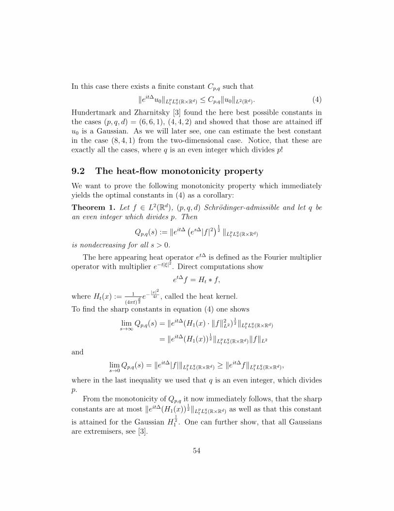
In this case there exists a finite constant Cp,q such that
‖eit∆u0‖LptLqx(R×Rd) ≤ Cp,q‖u0‖L2(Rd). (4)
Hundertmark and Zharnitsky [3] found the here best possible constants inthe cases (p, q, d) = (6, 6, 1), (4, 4, 2) and showed that those are attained iffu0 is a Gaussian. As we will later see, one can estimate the best constantin the case (8, 4, 1) from the two-dimensional case. Notice, that these areexactly all the cases, where q is an even integer which divides p!
9.2 The heat-flow monotonicity property
We want to prove the following monotonicity property which immediatelyyields the optimal constants in (4) as a corollary:
Theorem 1. Let f ∈ L2(Rd), (p, q, d) Schrodinger-admissible and let q bean even integer which divides p. Then
Qp,q(s) := ‖eit∆(es∆|f |2
) 12 ‖LptLqx(R×Rd)
is nondecreasing for all s > 0.
The here appearing heat operator et∆ is defined as the Fourier multiplieroperator with multiplier e−t|ξ|
2. Direct computations show
et∆f = Ht ∗ f,
where Ht(x) := 1
(4πt)d2e−|x|24t , called the heat kernel.
To find the sharp constants in equation (4) one shows
lims→∞
Qp,q(s) = ‖eit∆(H1(x) · ‖f‖2L2)
12‖LptLqx(R×Rd)
= ‖eit∆(H1(x))12‖LptLqx(R×Rd)‖f‖L2
and
lims→0
Qp,q(s) = ‖eit∆|f |‖LptLqx(R×Rd) ≥ ‖eit∆f‖LptLqx(R×Rd),
where in the last inequality we used that q is an even integer, which dividesp.
From the monotonicity of Qp,q it now immediately follows, that the sharp
constants are at most ‖eit∆(H1(x))12‖LptLqx(R×Rd) as well as that this constant
is attained for the Gaussian H121 . One can further show, that all Gaussians
are extremisers, see [3].
54

9.2.1 Proof sketch of the monotonicity property
By using that the heat kernel combined with the convolution builds a semi-group, the Cauchy-Schwarz inequality and
´Ht ∗ f =
´f one can show:
Lemma 2. For nonnegative functions f1, f2 ∈ L1(Rd), the quantity
Λf1,f2(s) :=
ˆRd
(es∆f1)12 (es∆f2)
12
is nondecreasing for all s > 0.
To shorten our notation we will from now on only look at dimension 1.The proof in 2 dimensions works in the same way.The next step is to prove the following representation of Strichartz-norms,which was shown in [3].
Lemma 3. For f ∈ L2(R) we have
‖eit∆f‖L6t,x(R×R) =
1
2√
3〈f ⊗ f ⊗ f, P (f ⊗ f ⊗ f)〉,
where P : L2(R3) → L2(R3) is the projection operator onto the subspace offunctions on R3 invariant under the isometries that fix the direction (1, 1, 1).
Here we defined (f ⊗ f ⊗ f)((x1, x2, x3)) := f(x1)f(x2)f(x3).
Proof sketch. To shorten our notation lets define F (X) := (f ⊗ f ⊗ f)(X).We expand
|eit∆f |6 =1
(4πt)3
ˆR3
ei3|x|2−2x(1,1,1)·η+|η|2
4t F (η)dη ·ˆR3
e−i3|x|2−2x(1,1,1)·ξ+|ξ|2
4t F (ξ)dξ,
integrate with respect to x and carry out a change of variables to obtain forF ∈ C∞0 (R3)ˆR|eit∆f |6dx =
2t
(4πt)3
ˆR
ˆR3
ˆR3
e−ix(1,1,1)·(η−ξ) ei|η|2−|ξ|2
4t F (η)F (ξ)dηdξdx
=2t
(4πt)3
ˆR3
ˆR3
2π · δ((1, 1, 1) · (η − ξ))ei|η|2−|ξ|2
4t F (η)F (ξ)dηdξ.
Doing the same in t leads toˆR
ˆR|eit∆f |6dxdt =
1
2π
ˆR3
ˆR3
δ((1, 1, 1) · (η − ξ))δ(|η|2 − |ξ|2)F (η)F (ξ)dηdξ
=: 〈F,AF 〉L2η(R3).
To finish the proof the following two steps are left to do:
55

1.) Show that A : C∞0 → L2 and extends to an operator from L2 into L2.
2.) Show that A = 12√
3P .
Comment on step 2: A change of variables shows that AF (for F ∈ C∞0 (R3))stays invariant under isometries that fix the direction (1, 1, 1), because thoseisometries don’t change the input of the δ-functions. By step 1 this extendsto all F ∈ L2(R3) and thus A maps into the range of P . Because A issymmetric it follows that A maps the complement of the range of P to 0and it remains to check, that A acts as the wanted multiple on the range ofP .
We can now conclude the monotonicity property:By using that every isometry ρ on R3 has the form ρ(x) = ρ(0) + ρx, whereρ is an orthogonal matrix, a change of variables shows that (et∆|F |2)(ρ·) =(et∆|Fρ|2) where Fρ = F (ρ·). Therefore we get
(es∆|f |2 ⊗ es∆|f |2 ⊗ es∆|f |2)(ρ·) = (es∆|F |2)(ρ·) = (es∆|Fρ|2),
because es∆ commutes with tensor products.Let O be the group of isometries on R3 that coincide with the identity on thespan of (1, 1, 1). One can than calculate, that for G ∈ L2(R3) the projectionP is given by
PG(·) =
ˆOG(ρ·)dH (ρ),
where dH denotes the right-invariant Haar probability measure onO. There-fore we have by the previous lemma and the above statements
Q6,6(s) =1
2√
3
ˆR3
(es∆|F |2)12
ˆO
(es∆|Fρ|2)12 dH =
1
2√
3
ˆO
Λ|F |2,|Fρ|2(s)dH ,
which is by lemma 2 and the positivity of dH nondecreasing. As previouslymentioned the proof for the case (p, q, d) = (4, 4, 2) works analogous. For(p, q, d) = (8, 4, 1) we use again, that the operators eit∆ and es∆ commutewith tensor products and therefore
‖eit∆(es∆|f |2)12‖2
L8tL
4x(R×R) = ‖eit∆(es∆(|f |2 ⊗ |f |2))
12‖L4
tL4x(R×R2),
which is nondecreasing by the 2-dimensional case.
56

Remark 4. One can use the same strategy as above to proof the monotonicityof the Strichartz norm for input which evolves according to a quadratic Mehlerflow. That is, for a bounded and compactly supported function f which ful-fils the assumptions of theorem 1 the quantity ‖eit∆(e−|·|
2etL|f |2)
12‖LptLqx(R×Rd),
where L = ∆− 〈x,∇〉, is nondecreasing for all s > 0.
9.3 Higher dimensions
It is already proven that for all nonendpoint (p 6= 2) Schrodinger-admissible(p, q, d) the best possible constant is attained (see Shao [5]), however theextremisers are in general not known. We would like to generalise theorem1 to all dimensions. Therefore we consider the case p = q = 2 + 4
d=: p(d).
Unfortunately p(d) is not an even integer for d ≥ 3 (then we would befinished). Our approach is to embed the Strichartz norm into a family ofnorms ||| · |||p which fulfil the statement of theorem 1 for even integers p. Forthis procedure we choose for f ∈ S(Rd) the norm
|||f |||pp :=
(p(d)
π
) d2 1
(2π)d+2
ˆRd
ˆRd
ˆ ∞0
ˆR
∣∣∣∣ˆRde−|z−
√ζξ|2ei(x·ξ−t|ξ|
2)f(ξ)dξ
∣∣∣∣p ζν−1
Γ(ν)dt dζ dz dx,
where ν := d(p−p(d))4
, and proof the following:
Theorem 5. As p tends to p(d), the norm |||f |||p converges to the Strichartznorm ‖eit∆f‖
Lp(d)t,x
for all f ∈ S(Rd). If p is an even integer, then
Qp(s) := |||(es∆|f |2)12 |||p
is nondecreasing for all s > 0.
Comment on the proof. The proof of this theorem turns out to be very sim-ilar to our proof of theorem 1. We again (compare to lemma 3) first showthat
|||f |||pp = Cd,p
ˆRpd2
F (X)PF (X)dX,
where P is the orthogonal projection onto functions on Rpd2 which are in-
variant under the action of O, the group of isometries that coincide with
the identity on W , the span of 11, . . . ,1d ∈ Rpd2 where for each 1 ≤ j ≤ d
1j := (ej, . . . , ej) and ej denotes the jth standard basis vector of Rd. Wethan again express P through the right-invariant Haar probability measureon O and use lemma 2 to prove the nondecreasingness.
57

Remark 6. It is possible to generalise lemma 2 to higher exponents then 1/2by multiplying with a polynomially growing factor. Bennett, Carbery, Christand Tao prove in [2], that for all α ∈ [1/2, 1] the quantity
sd(α−1/2)/2
ˆRd
(es∆f1)α(es∆f2)α,
where f1, f2 are functions which satisfies the assumptions of lemma 2, isnondecreasing for all s > 0.By replacing lemma 2 with this statement in the proof of theorem 1 and 5one also obtains these results for higher exponents.
References
[1] Bennett, J., Bez, N., Carbery, A. and Hundertmark, D., Heat-flowmonotonicity of Strichartz norms. Anal. PDE 2 (2009), no. 2, 147–158.
[2] Bennett, J., Carbery, A., Christ, M. and Tao, T., The Brascamp-Liebinequalities: finiteness, structure and extremals. Geom. Funct. Anal. 17(2009), no. 5, 1343–1415.
[3] Hundertmark, D. and Zharnitsky, V., On sharp Strichartz inequalitiesin low dimensions. Int. Math. Res. Not., (2006), article ID 34080.
[4] Keel, M. and Tao, T., Endpoint Strichartz estimates. Amer. J. Math.120 (1998), no. 5, 955–980.
[5] Shao, S., Maximizers for the Strichartz inequalities and the Sobolev-Strichartz inequalities for the Schrodinger equation. EJDE (2009), no. 3.
[6] Strichartz, R., Restrictions of Fourier transforms to quadratic surfacesand decay of solutions of wave equations. Duke Math. J. 44 (1977), no. 3,705-714.
Lisa Onkes, University of Bonnemail: [email protected]
58

10 Multidimensional van der Corpus and sub-
level set estimates
after A. Carbery, M. Christ, and J. Wright [2]A summary written by Guillermo Rey
10.1 Introduction
In this article the authors consider the principle:
If a function has a large derivative, then it changes rapidly andhence cannot spend too much time near any particular value.
Their main goal is to quantify this principle.Suppose u is a smooth real valued function on R and assume that u(k) ≥ 1
everywhere. According to the above principle the sublevel set x : |u(x)| ≤α should be decrease as α → 0, and the rate of decay should be faster forsmaller k.
One could also consider the oscillatory integral
I(λ) :=
ˆ b
a
eiλu(t) dt.
If the derivative of u is very small then we would expect the phase to beessentially constant, and hence eiλu(t) should not introduce much cancellation,at least for small λ. But when the derivative of u is large then we shouldexpect cancellation.
The authors give quantitative versions of these intuitive statements, fur-thermore their results will be uniform in a sense which we’ll describe later.
10.2 The one-dimensional case
Much more is known about the problems discussed in the introduction ifwe restrict the dimension to one. In fact, a very precise estimate is knownfor both questions. The following estimates can be found in an article byArhipov, Karacuba and Cubarikov in [1].
Proposition 1. If u is a smooth function satisfying uk(t) ≥ 1 on R, then
|t : |u(t)| ≤ α| ≤ (2e)((k + 1)!)1/kα1/k.
59

For the oscillatory integral estimate we have
Proposition 2. There exists an absolute constant C such that for any a < b,any k ≥ 2, and any smooth function u satisfying u(k) ≥ 1∣∣∣∣∣
ˆ b
a
eiλu(t) dt
∣∣∣∣∣ ≤ Ck|λ|−1k .
Let us give the main ideas of the proof of the first proposition:
1. First we letE = t : |u(t)| ≤ α.
One can show that it is possible to find k + 1 points: a0, . . . , ak whichare well-spaced in the sense that
|E|k ≤ (2e)k∏j 6=l
|aj − al| ∀l. (1)
2. Next, one can give a higher-order version of the Mean Value Theorem.It essentially says that one can find a point ζ such that
u(k)(ζ) = k!∑j
±u(aj)∏j 6=l
|aj − al|−1 (2)
3. Finally, since u(k) ≥ 1, we can reorganize (2) and use the estimate from(1) to conclude.
Proposition 2 follows from Proposition 1. Indeed, one can write
ˆ b
a
eiλu(t) dt =
ˆt∈(a,b): |u′(t)|≤β
eiλu(t) dt+
ˆt∈(a,b): |u′(t)|>β
eiλu(t) dt
=: I + II.
For I we can use Proposition 1 with v = u′, while for II one shouldexpploit the large cancellation arising from the fact that u′ is large on the setwhere we are integrating. In particular, the set t : |u′(t)| > β is a unionof O(k) intervals, and for each interval one can integrate by parts to exploitthe cancellation. To conclude one optimises β and the result follows.
60
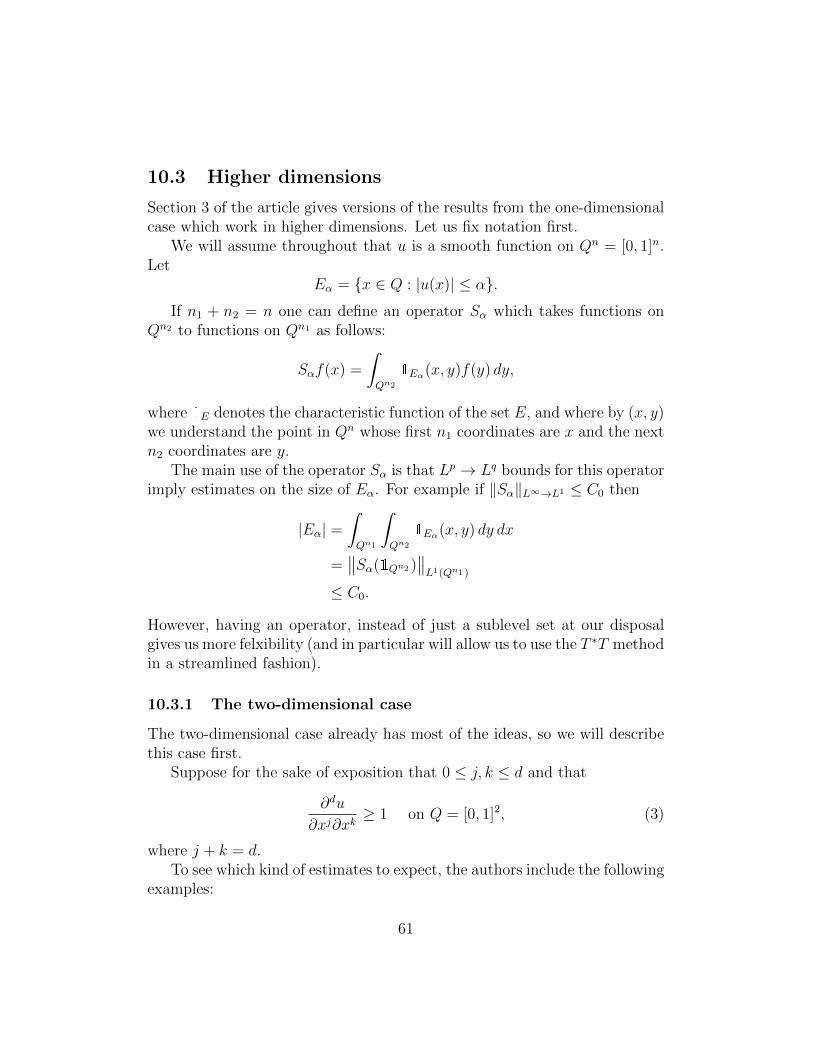
10.3 Higher dimensions
Section 3 of the article gives versions of the results from the one-dimensionalcase which work in higher dimensions. Let us fix notation first.
We will assume throughout that u is a smooth function on Qn = [0, 1]n.Let
Eα = x ∈ Q : |u(x)| ≤ α.If n1 + n2 = n one can define an operator Sα which takes functions on
Qn2 to functions on Qn1 as follows:
Sαf(x) =
ˆQn2
1Eα(x, y)f(y) dy,
where 1E denotes the characteristic function of the set E, and where by (x, y)we understand the point in Qn whose first n1 coordinates are x and the nextn2 coordinates are y.
The main use of the operator Sα is that Lp → Lq bounds for this operatorimply estimates on the size of Eα. For example if ‖Sα‖L∞→L1 ≤ C0 then
|Eα| =ˆQn1
ˆQn2
1Eα(x, y) dy dx
=∥∥Sα(1Qn2 )
∥∥L1(Qn1 )
≤ C0.
However, having an operator, instead of just a sublevel set at our disposalgives us more felxibility (and in particular will allow us to use the T ∗T methodin a streamlined fashion).
10.3.1 The two-dimensional case
The two-dimensional case already has most of the ideas, so we will describethis case first.
Suppose for the sake of exposition that 0 ≤ j, k ≤ d and that
∂du
∂xj∂xk≥ 1 on Q = [0, 1]2, (3)
where j + k = d.To see which kind of estimates to expect, the authors include the following
examples:
61
Proposition 3. For each j, k there exists a C < ∞ such that the followinghold:
1. If u(x, y) = −(x− y)d with d ≥ 2, then ‖Sα‖Lp→Lq ≥ Cα1/d.
2. If u(x, y) = xjyk, then ‖Sα‖Lp→Lq ≥ Cα1/jq.
3. If u(x, y) = xkyk, then ‖Sα‖Lp→Lq ≥ Cα1/kp′.
Proof. If f = 1(0,1) then Sαf ' α1/d, and hence the first result follows.The second result follows from noting that
Sαf(x) =
ˆ 1
0
f(y) dy
for x ∈ (0, α1/j).The second and third results are equivalent by duality so this finishes the
proof.
As a corollary, we have
sup ‖Sα‖Lp→Lq & αmin( 1
d, 1jq, 1kp′ ),
where the supremum is taken over all functions u which satisfy (3), so thisis the best we can expect for upper estimates.
The main result in the two-dimensional case is the following:
Theorem 4. There exists an absolute constant C so that if u satisfies (3)with j = k = 1, then
‖Sα‖L2→L2 ≤ C(α log(1/α)
)1/2 ∀α ∈ (0, 1/2).
Let us sketch the main ideas of the proof. We begin with the lemma
Lemma 5. For u as in the previous theorem, set E = Eα and let
E(y) = x : (x, y) ∈ E.
Then
|E(y1) ∩ E(y2)| ≤ 4α
|y1 − y2|. (4)
62

This can be seen as a two-dimensional version of 1Now the estimate follows from a T ∗T argument:
‖Sαf‖2 =
ˆ|Sαf(x)|2 dx
=
ˆ (ˆ1Eα(x, y)f(y) dy
)2
dx
=
ˆ ˆ ˆ1Eα(x, y1)f(y1)1Eα(x, y2)f(y2) dy1 dy2 dx
=
ˆ ˆ|E(y1) ∩ E(y2)|f(y1)f(y2) dy1 dy2
≤¨|y1−y2|≤4α
f(y1)f(y2) dy1 dy2 + 4α
¨|y1−y2|>4α
f(y1)f(y2)
|y1 − y2|dy1 dy2,
where we have used the previous lemma in the last line.The first summand is bounded by 4α‖f‖2
2, while for the second one wecan use Cauchy-Schwarz to conclude
4α
¨|y1−y2|>4α
f(y1)f(y2)
|y1 − y2|dy1 dy2 . 4α log(1/4α)‖f‖2
2
and the proof follows.For dimensions larger than two the authors use an induction argument,
but then the exponents behave much worse:
Theorem 6. For each n ≥ 1 and each multiindex β there exists an ε > 0and C <∞ such that for any real-valued smooth function satisfying ∂βu ≥ 1we have
|x ∈ Q : |u(x)| ≤ α| ≤ Cαε.
A similar version for the oscillatory integral estimate follows from thislast theorem.
10.4 Applications and further remarks
The results of this paper have certain combinatorial applications. Considerthe following problem:
Conjecture 7. There exists a constant ε0 > 0 such that for any E ⊂ Q =[0, 1]2 with |E| > 0 one can always find four points A,B,C,D ∈ E which are
63

the vertices of a rectangle with sides parallel to the axes and whose area is atleast ε0|E|2.
If the conjecture is true then Theorem 4 would be true without the log-arithmic term. On the other hand Theorem 4 implies that there exists sucha rectangle but with area at least
ε01
log |E|−1|E|2.
The authors describe further applications, we refer the reader to the orig-inal article.
References
[1] G.I. Arhipov, A.A. Karacuba and V.N. Cubarikov, Trigonometric In-tegrals, Math. USSR Izvestija 15, 2 (1980) 211 – 239.
[2] A. Carbery, M. Christ and J. Wright, Multidimensional van der Corputand sublevel set estimates. J. Amer. Math. Soc. 12 (1999), no. 4, 981–1015.
Guillermo Rey, MSUemail: [email protected]
64

11 Optimal Young’s inequality and its con-
verse: a simple proof
after F. Barthe [1]A summary written by Johanna Richter
Abstract
The sharp form of Young’s inequality for convolutions was firstproven by Beckner [2] and Brascamp and Lieb [3]. The first knownproof of the sharp reverse inequality for exponents less than 1 can alsobe found in [3]. We summarize Barthes [1] proof of Young’s inequality,which is rather elementary and gives the inequality and its converseat one time.
11.1 Introduction and main result
The classical Young’s inequality for convolutions states that
‖f ∗ g‖r ≤ ‖f‖p‖g‖q, (1)
if f ∈ Lp(R), g ∈ Lq(R) and p, q, r ≥ 1 satisfy 1/p + 1/q = 1 + 1/r. Forexponents 0 < p, q, r ≤ 1 and f, g ≥ 0 Leindler [4] found the reverse form
‖f ∗ g‖r ≥ ‖f‖p‖g‖q. (2)
Both inequalities are sharp, only if p = 1 or q = 1. In the other cases thebest constants were found by Beckner [2] for (1) and Brascamp and Lieb [3]for (1) and (2). They are attained when f and g are gaussian functions,f(x) = exp(−|p′|x2) and g(x) = exp(−|q′|x2). Throughout this summary weuse the convention 1/p+ 1/p′ = 1. Note that p′ < 0, if 0 < p < 1.
We will present an argument, which proves the following sharp, multidi-mensional Young’s inequality and its converse at one go.
Theorem 1. Let p, q, r > 0 satisfy 1/p+ 1/q = 1 + 1/r, let f ∈ Lp(Rn) and
g ∈ Lq(Rn) be non-negative and define Ct = t1/2t
|t′|1/2t′ for every t > 0.
(i) If p, q, r ≥ 1, then
‖f ∗ g‖r ≤(CpCqCr
)n‖f‖p‖g‖q. (3)
65

(ii) If p, q, r ≤ 1, then
‖f ∗ g‖r ≥(CpCqCr
)n‖f‖p‖g‖q. (4)
It is enough to prove Theorem 1 for n = 1. Via tensorisation arguments,it is possible to deduce the multidimensional case from the one-dimensional:if C is the best constant for R, then Cn is the best constant for Rn. This isdone for example in Beckner [2] (see Topic 2).
11.2 Reformulation of the problem
For n = 1 and p, q, r 6= 1 we obtain by a change of variables the following,equivalent form of Theorem 1:
Theorem 2. Let p, q, r > 0 satisfy 1/p + 1/q = 1 + 1/r, let f, g ∈ L1(R) be
non-negative and define c =√r′/q′, s =
√r′/p′ and K(p, q, r) = p1/2pq1/2q
r1/2r.
(i) If p, q, r > 1, then(ˆR
(ˆRf(cx− sy)1/pg(sx+ cy)1/qdx
)rdy
)1/r
≤ K(p, q, r)‖f‖1/p1 ‖g‖
1/q1 .
(ii) If p, q, r < 1, then(ˆR
(ˆRf(cx− sy)1/pg(sx+ cy)1/qdx
)rdy
)1/r
≥ K(p, q, r)‖f‖1/p1 ‖g‖
1/q1 .
It is enough to prove Theorem 2 for positive, continuous functions f, g ∈L1(R).
Indeed, for all 0 ≤ f ∈ L1(R) we find 0 ≤ fn ∈ L1(R), n ∈ N, suchthat fn ↑ f pointwise and fn(x) ≤ Mn exp(−εnx2) =: Fn(x) for some
Mn, εn > 0 and all n ∈ N. For m ∈ N let ϕm(x) = m√2π
exp(− (mx)2
2) and
define fn,m(x) = min(fn ∗ ϕm)(x), Fn(x). Note that the functions fn,m arepositive and continuous and that limm→∞ ‖fn,m − fn‖p = 0 for all p ≥ 1. Dothe same construction for 0 ≤ g ∈ L1(R).
If Theorem 2 holds for all fn,m and gn,m, then by the dominated conver-gence theorem, it is true for all fn and gn and by the monotone convergencetheorem, it is true for f and g.
66

11.3 The key element of the proof
Lemma 3. Let p, q, r > 1 satisfy 1/p + 1/q = 1 + 1/r and let f, F, g,G ∈L1(R) be positive, continuous functions, such that
´R f dx =
´R F dx and´
R g dx =´RGdx. Then
(ˆR
(ˆRf(cx− sy)1/pg(sx+ cy)1/qdx
)rdy
)1/r
≤ˆR
(ˆRF (cx− sy)r/pG(sx+ cy)r/qdy
)1/r
dx. (5)
Note that if p, q, r > 1 then P = p/r,Q = q/r,R = 1/r satisfy 0 <P,Q,R < 1 and 1/P + 1/Q = 1 + 1/R. Further, it is C =
√R′/P ′ = s, S =√
R′/Q′ = c. By applying Lemma 3 to p, q, r > 1 with suitable f, F, g,G, we
obtain for P,Q,R < 1 and f , F , g, G, where f(x) = f(−x), F (x) = F (−x)(ˆR
(ˆRF (Cx− Sy)1/PG(Sx+ Cy)1/Qdx
)Rdy
)1/R
=
(ˆR
(ˆRF (cx− sy)r/pG(sx+ cy)r/qdy
)1/r
dx
)r
≥ˆR
(ˆRf(cx− sy)1/pg(sx+ cy)1/qdx
)rdy
=
ˆR
(ˆRf(Cx− Sy)R/Pg(Sx+ Cy)R/Qdy
)1/R
dx. (6)
Proof of Lemma 3. The proof is based on a parametrization of functions.Due to the assumptions on f, F, g,G, there are two increasing bijectionsu, v ∈ C1(R) such that for all t
ˆ u(t)
−∞f(x) dx =
ˆ t
−∞F (x) dx,
ˆ v(t)
−∞g(x) dx =
ˆ t
−∞G(x) dx and
u′(t)f(u(t)) = F (t), v′(t)g(v(t)) = G(t). (7)
Construct another differentiable bijection Θ = RtTR : R2 → R2, using the
rotation R with matrix
(c −ss c
)and the bijection T (x, y) = (u(x), v(y)). Its
67
Jacobian JΘ at a point (X, Y ) is equal to JΘ(X, Y ) = u′(cX − sY )v′(sX +cY ).
Let I denote the left-hand side of inequality (5). We may assume I <∞,using the classical Young’s inequality (1). Thus, the duality between Lr andLr′
implies the existence of a positive function h ∈ Lr′(R), ‖h‖r′ = 1 such
that
I =
ˆR
ˆRf(cx− sy)1/pg(sx+ cy)1/qh(y) dx dy.
By the change of variables (x, y) = Θ(X, Y ) and an application of Holder’sinequality, we find
I ≤ˆR
(ˆRF (cX − sY )r/pG(sX + cY )r/qdY
)1/r
H(X)1/r′ dX,
where
H(X) =
ˆRh(a(X, Y ))r
′u′(cX − sY )s
2
v′(sX + cY )c2
dY and
a(X, Y ) = −su(cX − sY ) + cv(sX + cY ).
Using the arithmetic-geometric inequality, we obtain
u′(cX − sY )s2
v′(sX + cY )c2 ≤ s2u′(cX − sY ) + c2v′(sX + cY ) = ∂Y a(X, Y ).
Thus,
H(X) ≤ˆRh(a(X, Y ))r
′∂Y a(X, Y ) dY =
ˆRh(z)r
′dz = 1.
This proves the lemma.
11.4 Proof of Theorem 2
For the functions
f(x) = F (x) =√p/π exp(−px2), g(x) = G(x) =
√q/π exp(−qx2),
we obtain equality in Lemma 3 and both sides of (5) are equal to K(p, q, r).Substituting f, g by any two functions 0 < f, g ∈ C(R) such that
´R f dx =´
R g dx = 1, immediately leads to Theorem 2 for p, q, r > 1.As we showed in (6), Lemma 3 is valid for 0 < P,Q,R < 1, but with the
reverse inequality sign. Therefore, the assertion for exponents less than onefollows from (6), applyed to 0 < F ,G ∈ C(R) such that
´R F dx =
´RGdx =
1 and f(x) =√P/π exp(−Px2), g(x) =
√Q/π exp(−Qx2).
68

11.5 Extremizers
Theorem 4. Let p, q, r > 0 satisfy 1/p+ 1/q = 1 + 1/r and either p, q, r > 1or p, q, r < 1. Let further f, g ∈ L1(R) be non-negative and c, s and K =K(p, q, r) defined as above. Then(ˆ
R
(ˆRf(cx− sy)1/pg(sx+ cy)1/qdx
)rdy
)1/r
= K ‖f‖1/p1 ‖g‖
1/q1 (8)
if and only if there exist a, b ≥ 0, λ > 0 and y, z ∈ R such that for all x ∈ R
f(x) = a exp(−λp(x− y)2), g(x) = b exp(−λq(x− z)2). (9)
For the proof of Theorem 4 we need the following Lemma.
Lemma 5. Let m,n ∈ Z,m ≥ n, let αi ∈ R be positive and ui ∈ Rn fori = 1, . . . ,m. Assume that M > 0 ist the smallest possible constant such thatfor all non- negative functions fi ∈ L1(R), i = 1, . . . ,m, one has
ˆRn
m∏i=1
fi(〈x, ui〉)αi dx ≤Mm∏i=1
‖fi‖αi1 . (10)
If there ist equality in (10) for the functions f1, . . . , fm and g1, . . . , gm, thenthere ist equality for f1 ∗ g1, . . . , fm ∗ gm.
Sketch of the proof. Assume there is equality in (10) for f1, . . . , fm andg1, . . . , gm, with ‖fi‖1 = ‖gi‖1 = 1 for all i = 1, . . . ,m. A straightforwardcomputation shows that
M2 =
(ˆRn
m∏i=1
fi(〈x, ui〉)αi dx
)(ˆRn
m∏i=1
gi(〈x, ui〉)αi dx
)
≤M
ˆRn
m∏i=1
(fi ∗ gi)(〈x, ui〉)αi dx ≤M2.
This implies the assertion. Proof of Theorem 4. A simple calculation shows that functions of the form(9) satisfy (8).
Let p, q, r > 1 and 0 < f, g ∈ C(R) ∩ L1(R) satisfy (8) and´R f dx =´
R g dx = 1. If we choose F (x) =√p/π exp(−px2), G(x) =
√q/π exp(−qx2),
69

we obtain equality in (5) and therefore everywhere in the proof of Lemma3, especially in the arithmetic-geometric inequality. This leads us to thecondition u′(cx − sy) = v′(sx + cy) = µ for all x, y ∈ R and a constantµ > 0. Thus, u(t) = µ(t − y0), v(t) = µ(t − z0) for some y0, z0 ∈ R and by(7) we end up with µf(µ(t − y0)) =
√p/π exp(−pt2) and µg(µ(t − z0)) =√
q/π exp(−qt2).Now let f, g ∈ L1(R) be arbitrary, non-negative functions, satisfying (8).
By the (Lr, Lr′)-duality, (8) is equivalent to the existence of a non-negative
function h ∈ Lr′(R) such that f, g, and h = hr′
satisfy
ˆR
ˆRf(cx− sy)1/pg(sx+ cy)1/qh(y)1/r′ dx dy = K ‖f‖1/p
1 ‖g‖1/q1 ‖h‖
1/r′
1 .
Brascamp and Lieb [3] showed that F (x) = exp(−px2), G(x) = exp(−qx2)and H(x) = exp(−r′x2) have the same extremal property as f, g, h. Thus,by Lemma 5, the positive and continuous functions f ∗ F and g ∗ G satisfy(8). As we showed above, they are of the form (9) and so are f and g, byproperties of the Fourier transform.
The case p, q, r < 1 is very similar and is omitted here.
References
[1] Barthe, F., Optimal Young’s inequality and its converse: a simple proof.Geom. Funct. Anal. 8 (1998), no. 2, 234-242.
[2] Beckner, W., Inequalities in Fourier analysis. Ann. of Math. (2) 102(1975), no. 1, 159-182.
[3] Brascamp, H.J. and Lieb, E.H., Best constants in Young’s inequality,its converse and its generalization to more than three functions. Adv.Math. 20 (1976), 151-173.
[4] Leindler, L., On a certain converse of Holder’s inequality. Acta Sci.Math. Szeged, 33 (1972), 217-223.
Johanna Richter, University of Stuttgartemail: [email protected]
70

12 Extremizers of a Radon transform inequal-
ity
after M. Christ[4]A summary written by Joris Roos
Abstract
The Radon transform maps functions defined on Rd to functionson the affine Grassmann manifold Gd of affine hyperplanes in Rd.It satisfies a L(d+1)/d(Rd) → Ld+1(Gd) endpoint estimate. In thepresented article [4], all the extremizers of this inequality are identified.
12.1 Introduction
Let d ≥ 2. By Gd we denote the affine Grassmann manifold of all affinehyperplanes in Rd. Define the measure µ on Gd to be the pushforward ofdrdθ along the canonical two-to-one map
R× Sd−1 → Gd, (r, θ) 7→ x : x · θ = r.
Here dθ denotes the surface measure on Sd−1. The Radon transform is definedby integrating over affine hyperplanes as follows,
Rf(r, θ) =
ˆx·θ=r
f(x)dσr,θ(x),
where dσr,θ is the surface measure of the affine hyperplane x : x · θ = r.The point of departure in the presented article is the endpoint inequality
‖Rf‖Ld+1(Gd,µ) ≤ A‖f‖L(d+1)/d(Rd), (1)
whereA denotes the optimal constant of this estimate, A = supf 6=0
‖Rf‖Ld+1(Gd,µ)
‖f‖L(d+1)/d(Rd)
.
A function 0 6= f ∈ L(d+1)/d(Rd) is said to be an extremizer in the inequal-ity (1), if ‖Rf‖Ld+1(Gd,µ) = A‖f‖L(d+1)/d(Rd). Let A(d) denote the group of
affine, invertible maps φ : Rd → Rd. Also, let us write 〈x〉 = (1 + |x|2)1/2 forconvenience.
The main result of [4] is the following.
71

Theorem 1. Every extremizer of (1) is of the form
f(x) = c〈φ(x)〉−d,
where c ∈ C\0 and φ ∈ A(d).
This solves a special case of a conjecture of Baernstein and Loss [1]. Theresults of [4] also encompass two related operators, R] and C. Let us viewRd as Rd−1 × R1 with coordinates x = (x′, xd) ∈ Rd−1 × R1. Then we define
R]f(x) =
ˆRd−1
f(y′, xd + y′ · x′)dy′,
Cf(x) =
ˆRd−1
f(x′ − y′, xd −1
2|y′|2)dy′.
The operators R], C satisfy endpoint inequalities of the same form as (1)and the corresponding optimal constants are in fact equal to A and there isa corresponding theorem for the extremizers of these inequalites.The general outline for the proof of the main result is as follows.
(1) Show existence of radial extremizers. This follows by prior results ofthe author [5], [6] and the connection to the operator C.
(2) Show that every extremizer has the form f φ with φ ∈ A(d). Thisis done using an array of tools from symmetrization and inverse sym-metrization theory.
(3) Exhibit an additional symmetry of the inequality (1) under which theset of radial functions composed with affine, invertible transformationsis not invariant.
(4) Prove that every radial extremizer has the form c〈ax〉−d with c ∈C\0, a > 0. This is done by exploiting the additional symmetryfrom the previous step.
In the following we will briefly describe some of the main ingredients ofthe proof.
72
12.2 Some ingredients of the proof
12.2.1 Connection of R,R], C.
The operators R and R] are connected by a change of variables leading upto the identity
〈x′〉R]f(x) = Rf(r, θ),
where r = xd/〈x′〉 and θ = (−x′, 1)/〈x′〉. This can be used to show
‖R]f‖Ld+1(Rd) = ‖Rf‖Ld+1(Gd,µ).
The connection of R and C is also simple. Define a map Ψ : Rd → Rd byΨ(x′, xd) = (x′, xd − 1
2|x′|2) and let Ψ∗f = f Ψ. Then we have
C = Ψ∗ R Ψ∗.
The proof is again a change of variables.
12.2.2 Affine invariance.
A fundamental property of the inequality (1) is its affine invariance. Namelyfor every φ ∈ A(d) we have
‖R(f φ)‖Ld+1(Gd,µ)
‖f φ‖L(d+1)/d(Rd)
=‖Rf‖Ld+1(Gd,µ)
‖f‖L(d+1)/d(Rd)
. (2)
In particular, if f is an extremizer for (1), then so is f φ for every φ ∈ A(d).This identity is proven by associating R to a symmetric bilinear form. Definethe measure λ on Rd × Rd by
dλ(x, y) = limε→0+
1
2ε1|x·y−1|<εdxdy
It is then proven that
‖Rf‖Ld+1(Gd,µ) = supg 6=0
∣∣∣ ´Rd×Rd fgdλ∣∣∣‖g‖L(d+1)/d(Rd)
,
which implies the affine invariance (2).
73

12.2.3 An additional symmetry.
As alluded to above, there is an additional symmetry of the inequality (1)that is central to the analysis. Let us view Rd as Rd−2×R1×R1 and considercoordinates (u, s, t) ∈ Rd−2 × R1 × R1. Define
J f(u, s, t) = |s|−df(s−1u, s−1, s−1t),
Lf(u, s, t) = f(u, t, s).
Then we have ‖J f‖(d+1)/d = ‖f‖(d+1)/d. Moreover, L R] = R] J . Com-bining the last two equations gives
‖R]J f‖d+1
‖J f‖(d+1)/d
=‖R]f‖d+1
‖f‖(d+1)/d
.
In particular, if f is an extremizer for (1), then also J f is.
12.2.4 Drury’s identity.
We continue to use the coordinates x = (x′, xd) ∈ Rd−1×R1. Let ∆(x1, . . . , xd)be the (d−1)-dimensional volume of the simplex in Rd spanned by x1, . . . , xdin Rd and ∆′(x′1, . . . , x
′d) the (d − 1)-dimensional volume of the simplex in
Rd−1 spanned by x′1, . . . , x′d ∈ Rd−1. For functions f0, . . . , fd on Rd we define
R(f0, . . . , fd) =
ˆ
(Rd)d
∆(x1, . . . , xd)−1
ˆ
π(x1,...,xd)
f0 dσπ
d∏j=1
fj(xj)d∏i=1
dxi,
where π = π(x1, . . . , xd) is the affine hyperplane in Rd containing the pointsx1, . . . , xd. This is well-defined for all up to a measure-zero set of d-tuples(x1, . . . , xd) ∈ (Rd)d. Also, σπ denotes the surface measure of the hyperplaneπ. Drury’s identity now amounts to the following:
‖Rf‖d+1Ld+1(Gd,µ)
= R(f, . . . , f). (3)
An alternative form of this identity is required. For any (d + 1)-tuple x′ =(x′0, . . . , x
′d) in (Rd−1)d+1 in general position let v(x′) ∈ Rd be the unique
vector such that x′0 =∑d
j=1 vj(x′)x′j and
∑dj=1 vj(x
′) = 1. Then we have
R(f0, . . . , fd) =
ˆ
(Rd−1)d+1
∆′(x′1, . . . , x′d)−1
ˆ
Rd
f0(x′0, v(x′)·t)d∏j=1
fj(x′j, tj)dt
d∏j=0
dx′j.
(4)
74

Therefore combining (3), (4) yields
‖Rf‖d+1Ld+1(Gd,µ)
=
ˆ
(Rd−1)d+1
∆′(x′1, . . . , x′d)−1Tv(x′0,...,x
′d)(f(x′0, ·), · · · , f(x′d, ·))
d∏i=0
dx′i,
(5)where
Tv(F0, . . . , Fd) =
ˆRdF0(t · v)
d∏j=1
F0(tj)dt. (6)
12.2.5 A rearrangement inequality.
For a measurable set E ⊂ Rd let E∗ be the open ball centered at the originsuch that |E| = |E∗|. The symmetric decreasing rearrangement of a functionf on Rd is defined as
f(x) =
ˆ ∞0
1y:f(y)>t∗(x)dt.
Brascamp, Lieb and Luttinger [2] proved a generalization of the Riesz-Sobolevrearrangement inequality which implies in particular
Tv(F0, . . . , Fd) ≤ Tv(F ∗0 , . . . , F ∗d ). (7)
12.2.6 Burchard’s theorem.
The work of Burchard [3] implies the following characterization of the casesof equality in (7).
Theorem 2. Let v ∈ Rd\0. Suppose that F0, . . . , Fd are nonnegative,measurable functions on R1 and that Tv(F ∗0 , . . . , F ∗d ). Also assume that thelevel sets of the fj have measure zero and that
Tv(F0, . . . , Fd) = Tv(F ∗0 , . . . , F ∗d ). (8)
Then there exist cj ∈ R such that
fj(t) = f ∗j (t− cj)
for almost every t ∈ R and c0 =∑d
j=1 cjvj.
75

Exploiting the Drury-type identity (5) for f being an extremizer it isproven that (8) holds for Fj = (f φ)(x′j, ·) and v = v(x′0, . . . , x
′d) and every
φ ∈ A(d). However, to apply the theorem it is also required that the level setshave measure zero. A priori, it is not clear whether this is true for extremiz-ers of (1). Therefore, an alternative argument is necessary that circumventsusing this theorem directly but instead exploits a more fundamental variantof Theorem 2 that is used in its proof, combined with the rearrangementinequality (7).
References
[1] A. Baernstein and M. Loss, Some conjectures about Lp norms of k-planetransforms, Rend. Sem. Mat. Fis. Milano 67 (1997), 9???26 (2000).
[2] H. J. Brascamp, E. Lieb and J. M. Luttinger, A general rearrange-ment inequality for multiple integrals, J. Functional Analysis 17 (1974),227???237.
[3] A. Burchard, Cases of equality in the Riesz rearrangement inequality,Ann. of Math. (2) 143 (1996), no. 3, 499???527.
[4] M. Christ, Extremizers of a Radon transform inequality. Preprint, arXiv:1106.0719 (2011).
[5] M. Christ, Estimates for the k-plane transform, Indiana Univ. Math. J.33 (1984), no. 6, 891???910.
[6] M. Christ, On extremals for a Radon-like transform. Preprint, arXiv:1106.0728 (2011).
Joris Roos, University of Bonnemail: [email protected]
76
13 Existence of extremizers for a family of
extension operators
after L. Fanelli, L. Vega and N. Visciglia [2]A summary written by Julien Sabin
Abstract
We present a general method to obtain the existence of optimizersfor a class of variational problems coming from extension operators,for which optimizing sequences exhibit a loss of compactness.
13.1 Introduction
Let X ⊂ RN and µ a Borel measure on X. Typically, one considers asubmanifold of RN together with its induced Lebesgue measure. We definethe extension operator T associated to (X,µ) as
Tf(x) :=
ˆX
f(ξ)eix·ξ dµ(ξ), ∀x ∈ RN ,
for all f ∈ L1(X,µ). Obviously, T is a continuous linear operator fromL1(X,µ) to C0
b (RN), the set of all bounded continuous functions on RN .Such operators arise naturally in the context of Strichartz estimates [9, 3],and more generally in harmonic analysis following Stein [8]. The typicalresult that is proved in these contexts is the boundedness of T as an operatorfrom L2(X, dµ) to Lp(RN) for some 1 ≤ p ≤ +∞. This means that thereexists C > 0 such that for all f ∈ (L1 ∩ L2)(X,µ) we have the bound
||Tf ||Lp(RN ) ≤ C ||f ||L2(X,µ) , (1)
and once such a bound is proved, this allows to extend T uniquely by densityfrom (L1 ∩ L2)(X,µ) to L2(X,µ).
Once we know that the operator T is bounded from L2(X,µ) to Lp(RN),it is a natural question to ask about the existence of extremizers, that isfunctions f 6= 0 such that
||Tf ||Lp(RN )
||f ||L2(X,µ)
= suph6=0
||Th||Lp(RN )
||h||L2(X,µ)
= ||T ||L2(X,µ)→Lp(RN ) . (2)
77

One difficulty to prove the existence of extremizers is the presence of a non-compact group of symmetry leaving the quotient ||Tf ||Lp / ||f ||L2 invariant.Indeed, for any x0 ∈ RN and for any f ∈ L2(X,µ) we define
gx0f(ξ) := f(ξ)eix0·ξ, ∀ξ ∈ X.
It satisfies ||gx0f ||L2(X,µ) = ||f ||L2(X,µ), and has the following intertwinningproperty with the operator T :
Tgx0 = τx0T,
where τx0h(x) := h(x + x0). In particular, this implies that ||Tgx0f ||Lp =||Tf ||Lp for all f . From this observation, one cannot hope for the pre-compactness of all maximizing sequences for the problem (2): indeed if itwere the case, there would exist an extremizer f∗ and the sequence (gxnf∗)for any |xn| → ∞ would be a maximizing sequence which is not precompact.
In this note, we present a method due to Fanelli, Vega, and Visciglia[2] that allows to prove the existence of extremizers for a general family ofextension operators, despite the difficulty just mentioned. Their method relyon the observation that it is enough to find a single non-trivial weak limitof a maximizing sequence, as was already emphasized by Brezis and Lieb[6, 1]. This principle is abstractly stated in Proposition 1 below. Then,this principle is applied to two situations: the finite volume case µ(X) <∞considered in [2] and an example in the infinite volume setting when X is aparaboloid.
13.2 An abstract result on the existence of extremizers
The method of Fanelli, Vega, and Visciglia is based on the following proposi-tion giving a sufficient condition on the existence of maximizers for a generalclass of linear operators.
Proposition 1. Let H a Hilbert space and T 6= 0 a bounded linear operatorfrom H to Lp(RN) for some 2 < p <∞. Let (fn) ⊂ H a sequence satisfying
1. ||fn||H = 1 for all n;
2. ||Tfn||Lp → ||T ||H→Lp;
3. fn f∗ 6= 0 in H;
78

4. Tfn → Tf∗ a.e. on RN .
Then, the sequence (fn) converges strongly in H to f∗. In particular, ||f∗||H =1 and ||Tf∗||Lp = ||T ||H→Lp.
Remark 2. The first two conditions on the sequence (fn) are the definitionof a maximizing sequence. In a concrete situation, one thus only has to checkthe last two conditions.
Proof. Define rn = fn − f∗. We thus have rn 0 and Trn → 0 a.e. on RN .This implies that
1 = ||fn||2H = ||f∗||2H + ||rn||2H + o(1).
Furthermore, by the Brezis-Lieb lemma [1], we have
||T ||pH→Lp + o(1) = ||Tfn||pLp = ||Tf∗||pLp + ||Trn||pLp + o(1).
As a consequence, we deduce that
||T ||pH→Lp = ||Tf∗||pLp + ||Trn||pLp + o(1) ≤ ||T ||pH→Lp (||f∗||pH + ||rn||pH) + o(1).
Since T 6= 0 and p > 2, this leads to
1 ≤ ||f∗||pH + ||rn||pH + o(1) ≤ (||f∗||2H + ||rn||2H)p/2 + o(1) = 1 + o(1).
In the limit n → ∞, the previous inequalities become equalities, and sinceap + bp = (a2 + b2)p/2 if and only if a = 0 or b = 0, we infer that ||f∗||H = 0 orlimn→∞ ||rn||H = 0. However, we assumed that f∗ 6= 0, which concludes theproof.
13.3 Application to extension operators in the finitevolume setting
We now apply the abstract previous proposition to the context of extensionoperators. As we have already mentioned, we just have to check the last twoconditions of Proposition 1 for maximizing sequences associated to extensionoperators. These two conditions are not satisfied for any (X,µ) and we haveto add some assumptions ensuring that they hold. This is summarized in thefollowing result.
79

Theorem 3. Let (X,µ) be such that´X
(1 + |ξ|2) dµ(ξ) <∞. Define
p0 = infp ≥ 1, T satisfies (1).
Then, for any p > max(2, p0) (with the convention that p = ∞ if p0 = ∞),there exists f ∈ L2(X,µ) with ||f ||L2(X) = 1 satisfying
||Tf ||Lp(RN ) = ||T ||L2(X)→Lp(RN ) .
Remark 4. Under the assumption that µ(X) <∞, T automatically satisfies(1) for p =∞ by the Cauchy-Schwarz inequality. The fact that p0 <∞ maydepend on additional properties of (X,µ) that we do not discuss here. Thereare several cases for which we know that p0 <∞ however [8, 11, 9].
The proof distinguishes between the cases p < ∞ and p = ∞. In thecase p <∞, we apply Proposition 1, while the case p =∞ requires a specialtreatment.
Proof in the case p <∞. Since the statement of the theorem obviously holdswhen µ = 0, we may assume that µ 6= 0 and hence T 6= 0. Let (fn) ⊂L2(X,µ) a sequence such that ||fn||L2(X) = 1 and
||Tfn||Lp(RN ) → ||T ||L2(X)→Lp(RN ) .
We first check condition (3) of Proposition 1, with the sole assumption thatµ(X) < ∞. Indeed, in this case T is bounded from L2(X) to L∞(RN) asalready mentioned. Let p such that p0 < p < p < ∞. By the Holderinequality and the definition of p0, there exists 0 < θ < 1 such that
||Tfn||Lp(RN ) ≤ ||Tfn||θLp(RN ) ||Tfn||
1−θL∞(RN )
≤ ||T ||θL2(X)→Lp(RN ) ||fn||θL2(X) ||Tfn||
1−θL∞(RN ) .
Since ||Tfn||Lp(RN ) → ||T ||L2(X)→Lp(RN ) 6= 0, we deduce from the last inequalitythat there exists ε0 > 0 such that
||Tfn||L∞(RN ) ≥ ε0 > 0
for n large enough. Hence, there exists (xn) ⊂ RN such that
|Tfn(xn)| ≥ ε0/2 > 0
80

for n large enough (when µ(X) < ∞, L2(X,µ) ⊂ L1(X,µ) and Tfn is abounded continuous function on RN for any n). Since
Tfn(xn) = (τxnTfn)(0) = (Tgxnfn)(0),
the sequence hn := gxnfn still satisfies ||hn||L2(X) = 1, ||Thn||Lp(RN ) → ||T ||L2(X)→Lp(RN )
with the additional property that
|Thn(0)| ≥ ε0/2 > 0
for n large enough. Since (hn) is bounded in L2(X,µ), we may assume thathn h∗ in L2(X,µ) up to a subsequence. Now
|〈1, h∗〉L2(X)| = limn→∞
|〈1, hn〉L2(X)| = limn→∞
∣∣∣∣ˆX
hn(ξ) dµ(ξ)
∣∣∣∣ = limn→∞
|Thn(0)|
and this implies that h∗ 6= 0, which is exactly condition (3) of Proposition1. To finish the proof of the theorem, we thus have to check condition (4) ofProposition 1, and this is where the assumption
´X|ξ|2dµ(ξ) appears. Indeed,
under this assumption, the sequence (Thn) actually belongs to C1(RN) withthe uniform bounds
||Thn||L∞(RN ) ≤ µ(X)1/2 ||hn||L2(X) = µ(X)1/2,
||∇xThn||L∞(RN ) ≤(ˆ
X
|ξ|2 dµ(ξ)
)1/2
which implies by the Ascoli-Arzela theorem that the sequence (Thn) con-verges uniformly on all compact sets of RN towards a continuous boundedfunction φ. To prove condition (4), we thus have to check that φ = Th∗. Forany ψ ∈ C∞0 (RN), we have by Fubini’s theorem
〈φ, ψ〉 = limn→∞〈Thn, ψ〉 = lim
n→∞〈hn, ψ|X〉L2(X) = 〈h∗, ψ|X〉L2(X) = 〈Th∗, ψ〉,
where we have used that ψ|X ∈ L2(X,µ) since µ is a finite Borel measure onX. This finishes the proof of the theorem.
Proof in the case p =∞. We define the sequence (hn) in the fashion as inthe case p <∞, except that we need the additional property that
||Thn||L∞(RN ) ≥ |Thn(0)| = |Tfn(xn)|≥ (1− 1/n) ||Tfn||L∞(RN ) = (1− 1/n) ||Thn||L∞(RN ) .
81

Again by the Ascoli-Arzela theorem, (Thn) converges to Th∗ uniformly onall compact sets of RN , and in particular
||Th∗||L∞(RN ) ≥ |Th∗(0)| = lim
n→∞|Thn(0)| = ||T ||L2(X)→L∞(RN ) .
On the other hand we have
||Th∗||L∞(RN ) ≤ ||T ||L2(X)→L∞(RN ) ||h∗||L2(X) ,
which implies that ||h∗||L2(X) ≥ 1 since T 6= 0. We always have ||h∗||L2(X) ≤ 1
by weak convergence, hence ||h∗||L2(X) = 1 and hn → h∗ strongly in L2(X),and hence h∗ is a maximizer.
Remark 5. The previous proofs show that we have actually the strongerresult that any maximizing sequence is pre-compact in L2(X,µ) up to theaction of symmetry group G = gx0 , x0 ∈ RN.
13.4 An application in infinite volume: Strichartz es-timates
As we saw in the previous proofs, the finite volume condition µ(X) < ∞ iscrucial, in particuliar to find a non-trivial weak limit h∗ via a uniform lowerbound on ||Thn||L∞(RN ). In this section we give an example on how to obtainsuch a lower bound in the infinite volume situation of Strichartz estimates.In this case (and in all of this section), the set X is a paraboloid
X = (ω, ξ) ∈ R× Rd, ω = |ξ|2, (3)
and the measure µ is given by the push-forward relationˆX
f(ω, ξ) dµ(ω, ξ) =
ˆRdf(|ξ|2, ξ) dξ. (4)
Strichartz estimates [9] state that there exists C > 0 such that
||Tf ||L2+4/d(Rd+1) ≤ C ||f ||L2(X) , (5)
for all f ∈ (L1 ∩ L2)(X,µ). Furthermore, a simple scaling argument showsthat p = 2 + 4/d is the only exponent such that (1) holds for this choice of(X,µ). In particular, it is hopeless to get a lower bound on ||Tfn||L∞(RN ) as
82
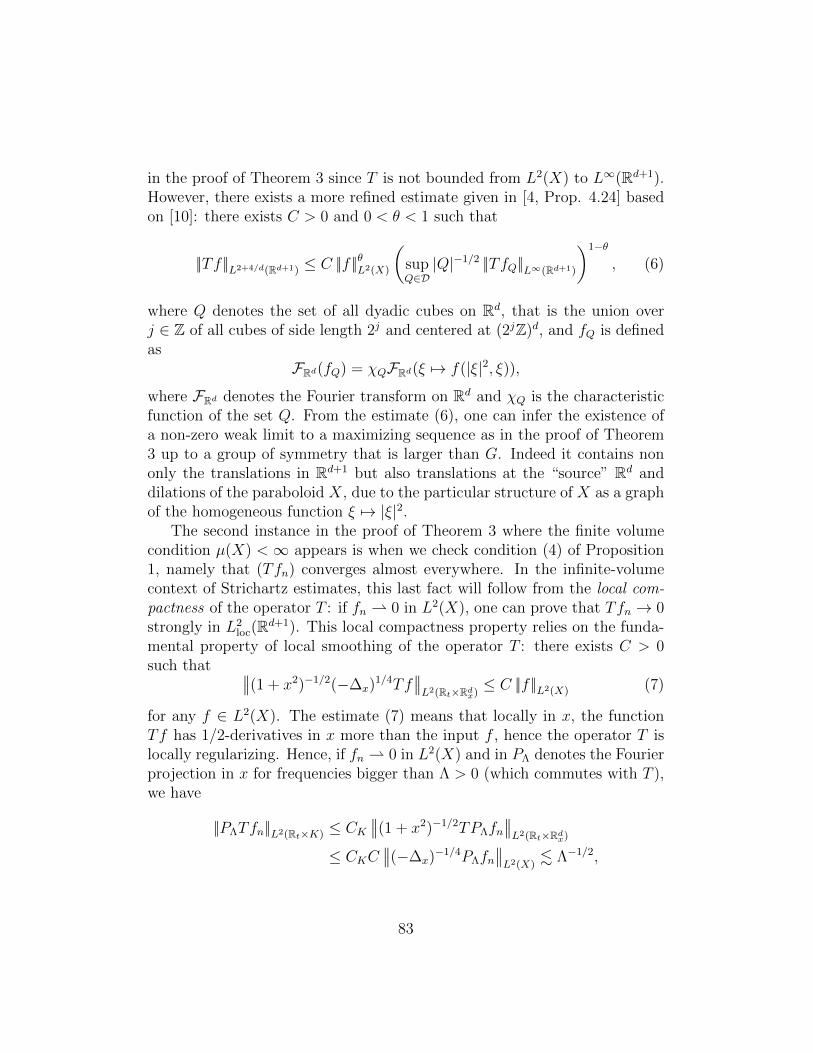
in the proof of Theorem 3 since T is not bounded from L2(X) to L∞(Rd+1).However, there exists a more refined estimate given in [4, Prop. 4.24] basedon [10]: there exists C > 0 and 0 < θ < 1 such that
||Tf ||L2+4/d(Rd+1) ≤ C ||f ||θL2(X)
(supQ∈D|Q|−1/2 ||TfQ||L∞(Rd+1)
)1−θ
, (6)
where Q denotes the set of all dyadic cubes on Rd, that is the union overj ∈ Z of all cubes of side length 2j and centered at (2jZ)d, and fQ is definedas
FRd(fQ) = χQFRd(ξ 7→ f(|ξ|2, ξ)),
where FRd denotes the Fourier transform on Rd and χQ is the characteristicfunction of the set Q. From the estimate (6), one can infer the existence ofa non-zero weak limit to a maximizing sequence as in the proof of Theorem3 up to a group of symmetry that is larger than G. Indeed it contains nononly the translations in Rd+1 but also translations at the “source” Rd anddilations of the paraboloid X, due to the particular structure of X as a graphof the homogeneous function ξ 7→ |ξ|2.
The second instance in the proof of Theorem 3 where the finite volumecondition µ(X) <∞ appears is when we check condition (4) of Proposition1, namely that (Tfn) converges almost everywhere. In the infinite-volumecontext of Strichartz estimates, this last fact will follow from the local com-pactness of the operator T : if fn 0 in L2(X), one can prove that Tfn → 0strongly in L2
loc(Rd+1). This local compactness property relies on the funda-mental property of local smoothing of the operator T : there exists C > 0such that ∣∣∣∣(1 + x2)−1/2(−∆x)
1/4Tf∣∣∣∣L2(Rt×Rdx)
≤ C ||f ||L2(X) (7)
for any f ∈ L2(X). The estimate (7) means that locally in x, the functionTf has 1/2-derivatives in x more than the input f , hence the operator T islocally regularizing. Hence, if fn 0 in L2(X) and in PΛ denotes the Fourierprojection in x for frequencies bigger than Λ > 0 (which commutes with T ),we have
||PΛTfn||L2(Rt×K) ≤ CK∣∣∣∣(1 + x2)−1/2TPΛfn
∣∣∣∣L2(Rt×Rdx)
≤ CKC∣∣∣∣(−∆x)
−1/4PΛfn∣∣∣∣L2(X)
. Λ−1/2,
83

for any compact K ⊂ Rd, meaning that the large frequency part of Tfn issmall in L2
loc(Rd+1). On the other hand,
(1− PΛ)Tfn(t, x) =
ˆ|ξ|≤Λ
eit|ξ|2−ix·ξfn(ξ) dξ,
converges to 0 for any fixed (t, x) ∈ R× Rd since ξ 7→ χ(|ξ| ≤ Λ)eit|ξ|2−ix·ξ ∈
L2(Rdξ) and (fn) converges weakly to zero in L2(Rd). This is how we prove
condition (4) in the case of the paraboloid. Together with Proposition 1, thisleads to the
Theorem 6. Assume X is the paraboloid (3) together with the measure (4).Then, the Strichartz estimate (5) has optimizers.
Remark 7. This result has been proved by Kunze [5] in d = 1 and by Shao [7]in d ≥ 2, using a profile decomposition. Our last proof shows that extractinga single non-trivial profile is enough to obtain the existence of extremizers.
Remark 8. Strichartz estimates also hold when replacing L2+4/d(R×Rd) byLptL
qx(R×Rd) with 2/p+ d/q = d/2, 2 ≤ q ≤ 2d/(d− 2) if d ≥ 3, 2 ≤ q <∞
if d = 2, and 2 ≤ q ≤ ∞ if d = 1. A similar proof shows the existence ofoptimizers when q is not equal to the endpoint q = 2d/(d− 2) for d ≥ 3 andq = ∞ for d = 1, 2. The existence of optimizers at the endpoint is an openproblem.
References
[1] H. Brezis and E. H. Lieb, A relation between pointwise convergenceof functions and convergence of functionals, Proceedings of the AmericanMathematical Society, 88 (1983), pp. 486–490.
[2] L. Fanelli, L. Vega, and N. Visciglia, On the existence of maxi-mizers for a family of restriction theorems, Bull. Lond. Math. Soc., 43(2011), pp. 811–817.
[3] M. Keel and T. Tao, Endpoint Strichartz estimates, Amer. J. Math.,120 (1998), pp. 955–980.
[4] R. Killip and M. Visan, Nonlinear Schrodinger equations at criticalregularity, Evolution equations, 17 (2013), pp. 325–437.
84
[5] M. Kunze, On the existence of a maximizer for the Strichartz inequal-ity, Commun. Math. Phys., 243 (2003), pp. 137–162.
[6] E. H. Lieb, Sharp constants in the Hardy–Littlewood–Sobolev and re-lated inequalities, Ann. Math., 118 (1983), pp. 349–374.
[7] S. Shao, Maximizers for the Strichartz inequalities and the Sobolev-Strichartz inequalities for the Schrodinger equation, Electronic J. of Dif-ferential Equations, (2009), pp. 1–13.
[8] E. M. Stein, Oscillatory integrals in Fourier analysis, in Beijing lec-tures in harmonic analysis (Beijing, 1984), vol. 112 of Ann. of Math.Stud., Princeton Univ. Press, Princeton, NJ, 1986, pp. 307–355.
[9] R. Strichartz, Restrictions of Fourier transforms to quadratic sur-faces and decay of solutions of wave equations, Duke Math. J., 44 (1977),pp. 705–714.
[10] T. Tao, A sharp bilinear restriction estimate for paraboloids, Geometric& Functional Analysis GAFA, 13 (2003), pp. 1359–1384.
[11] P. A. Tomas, A restriction theorem for the Fourier transform, Bull.Amer. Math. Soc., 81 (1975), pp. 477–478.
Julien Sabin, Universite Paris-Sud, Orsayemail: [email protected]
85

14 The Sharp Hausdorff-Young Inequality
after W. Beckner [1]A summary written by Mateus Sousa
Abstract
We study multiplier inequalities in the Hermite semigroup and usethe classical central limit theorem to obtain the sharp constant for theHausdorff-Young inequality through a limiting argument.
14.1 Introduction
For f ∈ L1(Rd) we consider the Fourier transform given by
F(f)(ξ) = f(ξ) :=
ˆRdf(x)e2πix·ξdx,
which extends to a bounded operator from Lp(Rd) to its dual space Lp′(Rd),
1 ≤ p ≤ 2, satisfying the classical Hausdorff-Young inequality
‖f‖p′ ≤ ‖f‖p. (1)
Inequality (1) is obtained from interpolation between the L1 and L2 cases,which are both sharp from the facts that for p = 1 any nonnegative functionattains equality in (1) and F extends as a unitary operator in L2.
Our main goal is to prove the sharp version of (1) for the remainingexponents, which is the following:
Theorem 1. For 1 < p < 2, and f ∈ Lp(Rd)
‖f‖p′ ≤ Adp‖f‖p, (2)
where Ap = (p1/p/p′1/p′)1/2.
The first observation to make is that the product structure of the Fouriertransform will make Theorem 1 follow directly from the case d = 1 andLemma 3 below, so we only need to consider the 1-dimensional case.
Another important observation is that the constant Adp is sharp because
it is attained for the function f(x) = e−π|x|2. In fact, gaussian functions are
86

the only maximizers of (2), but we do not address this question here and theinterested reader can check reference [2].
To prove the 1-dimensional case, we consider for ω ∈ C the operator Tωwhich acts in Hermite polynomials by
TωHm(x) = ωmHm(x),
where
Hm(x) =
ˆ(x+ iy)mdµ(y)
and
dµ(x) =1√2πe−x
2/2dx.
Tω can be expressed as an integral operator on L2(dµ) by
Tω(x, y) = (1− ω2)−1/2 exp
−ω
2(x2 + y2)
2(1− ω2)+
ωxy
1− ω2
,
(Tωg)(x) =
ˆTω(x, y)g(y)dµ(y).
The main property we need from Tω is the following result:
Theorem 2. For ω = i√p− 1 and 1 < p < 2, Tω extends to a bounded
operator from Lp(dµ) to Lp′(dµ) and
‖Tωg‖Lp′ (dµ) ≤ ‖g‖Lp(dµ). (3)
Now a simple change of variables shows that (3) holding for polynomialsg(x) is equivalent to the 1-dimensional case of (2) holding for functions of theform f(x) = g(
√2πpx)e−πx
2, which yields both theorems since they would
hold for a dense set of functions.
14.2 Discrete analogue of Tω
To prove Theorem 2, we use the classical central limit (CLT) theorem to getthe normal distribution dµ as a weak-? limit of Bernoulli trials.
Let dν(x) be a probability measure in R such that
ˆxdν(x) = 0,
ˆx2dν(x) = 1.
87

If we define nun as the n-fold convolution of the measure dν(√nx) with
itself, the classical central limit gives us that for every bounded continuousfunction h
limn→∞
ˆh(x)dνn(x) = lim
n→∞
ˆh(x1+···+xn√
n)dν(x1) · · · dν(xn)
=
ˆh(x)dµ(x)
(4)
For the case of a compactly supported measure dν, the convergence in(4) is also holds for functions h with polynomial growth. In particular, if weconsider a Bernoulli trial, i.e, a measure dν that gives weight 1/2 to x = ±1,for every polynomial h and 1 ≤ p <∞ we have
limn→∞
‖h‖Lp(dνn) = ‖h‖Lp(dµ). (5)
In order to establish (3) we define an analogue of the operator Tω forthe product measure dνn(x1, · · · , xn) = dν(
√nx1) × · · · × dν(
√nxn). Since
every function in the space Lp(dνn) can be seen as a polynomial of degree 1(in an almost everywhere sense) in each variable xk, we can define for every1 ≤ k ≤ n operators
Cn,k : a+ bxk 7→ a+ ωbxk,
where a and b are functions of the remaining n− 1 variables, and
K = Kn = Cn,n · · · Cn,1.
For the case k = n = 1 the operator K is simply the operator Tω as seenin Lp(dν), because H0(x) = 1 and H1(x) = x and so
Tw(aH0 + bH1) = aH0 + bωH1 = K(a+ bx).
The operator K works as a discrete analogue of Tω for the product mea-sure space in Lp(dνn). Now in order to get (3) we prove bounds for K andcompare what happens to Tωg and Kngn, where g is a polynomial and gn arefunctions associated to g given in terms of basic symmetric functions.
88

14.3 Bounds for the discrete analogue
To get bounds for Kn we just need to look at the case n = 1, because of thefollowing result about product of operators.
Lemma 3. Let T1 and T2 be two integral operators defined by kernels suchthat for every (f1, f2) ∈ Lp(dρ1)× Lp(dρ2)
‖T1f1‖Lp(dλ1) ≤ ‖f1‖Lq(dρ1),
‖T2f2‖Lp(dλ2) ≤ ‖f2‖Lq(dρ2)
for σ-finite measures λ1, λ2, ρ1, ρ2 and 1 ≤ p ≤ q. Then the integral operatorassociated to the product T1T2 maps Lp(dρ1 × dρ2) to Lq(dλ1 × dλ2) withnorm 1.
Lemma 3 is simple to get just applying Fubini’s theorem and Minkowski’sintegral inequality (which is the reason behind the p ≤ q), and with this inhand we just need to bound Cn,1 for each n. For that the case C = C1,1 thatis equivalent to the following result
Lemma 4. Let a, b ∈ C and 1 < p < 2. If we set ω = i√p− 1 then
|a+ ωb|p′ + |a− ωb|p′
2
1/p′
≤|a+ b|p + |a− b|p
2
1/p
.
Now to bound general Cn,1, and therefore Kn, one just needs to noticethat it follows straight from Lemma 4 that for any α > 0
‖Cg‖Lp′ (dνα) ≤ ‖g‖Lp(dνα),
where dνα(x) = dν(αx). Therefore, setting α =√n will give the desired
norm 1 of Kn. To finish things we just need to look at the interplay betweenK acting on symmetric functions and Tω acting on polynomials.
14.4 Hermite polynomials, symmetric functions andthe result
Let σn,j(x1, · · · , xn) be the basic symmetric functions, that is
σn,j(x1, · · · , xn) =∑
m1<···<mj
xm1 · · · xmj .
89

One can check that the functions ϕn,j = j!σn,j form an orthonormal basisfor the space of all the symmetric functions with respect to the L2(dνn)norm, and it follows from the definition that they are also eigenfunctions ofthe operator K, that is
Kϕn,j = ωjϕn,j. (6)
The generating function for the ϕn,j is given by
T (x1 · · · , xn, t) =n∏k=1
(1 + xkt)
=n∑j=0
ϕn,j(x1, · · · , xn)
j!tj.
For the Hermite polynomials the generating function is given by
T(x, t) =∞∑m=0
Hm(x)
m!tm.
If we consider the case x = x1 + · · ·+xn where each xk is either −1/√n or
1/√n, which is the set to consider when dealing with the measures dνn and
dνn, then one can look at the relations between T and T and get formulasrelating each each ϕn,l and the symmetrized functions Hm(x1+· · ·+xn) givenby Hermite polynomials, which is the following
ϕn,j(x1, · · · , xn) = Hj(x1 + · · ·+ xn) +1
n
bj/2c∑l=1
aj,lHj−2l(x1 + · · ·+ xn), (7)
where the coefficients aj,l are bounded with respect to n for fixed j (seeAppendix 1 of [1]).
Relation (7) means that for large values of n the main term of ϕn,j comesfrom Hj(x1 + · · ·+ xn). In fact it follows from (6) and (7) that
TωHj(x1 + · · ·+ xn)−Kϕn,j(x1, · · · , xn) =ωj
n
bj/2c∑l=1
aj,lHj−2l(x1 + · · ·+ xn),
and any Lp(dνn)-norm of the right-hand side goes to zero as n tends toinfinity because of (5).
90

Now we consider a polynomial g. Since the Hermite polynomials generatethe space of all polynomials (they are linearly independent and each Hm hasdegree m), we can write g as a linear combination of Hermite polynomials
g(x) =M∑m=0
bmHm(x).
We define for each n ∈ N the symmetric function
gn(x1, · · · , xn) =M∑m=0
bmϕn,m(x1, · · · , xn).
From (7) we get that
Tωg(x1 + · · ·+ xn)−Kgn(x1, · · · , xn) =M∑m=0
bmωm
n
bm/2c∑l=1
am,lHm−2l,
hence from the triangle inequality and the convergence to zero of the Lp(dνn)norms mentioned above, we get for every polynomial g that
limn→∞
|‖Tωg‖Lp(dνn) − ‖Kgn‖Lp(dνn)| = 0. (8)
Now if we set ω = i√p− 1, from Lemmas 3 and 4 we have
‖Kgn‖Lp′ (dνn) ≤ ‖gn‖Lp(dνn),
and from this last inequality, combined with (5) and (8), we get for everypolynomial g that
‖Tωg‖Lp′ (dµ) ≤ ‖g‖Lp(dµ),
which yields the desired result.
References
[1] W. Beckner, Inequalities in Fourier Analysis. Annals of Mathematics102 (1975), no. 1, 159–182.
[2] E. Lieb, Gaussian kernels have only gaussian maximizers. InventionesMathematicae 102 (1990), no. 1, 179–208.
Mateus Sousa, IMPAemail: [email protected]
91

15 A mass-transportation approach to sharp
Sobolev and
Gagliardo-Nirenberg inequalities
after D. Cordero-Erausquin, B. Nazaret, C. Villani [?].A summary written by Gennady Uraltsev.
Abstract
We show an elementary proof of Sobolev’s inequality on Rn withsharp constants for arbitrary norms on Rn. Mass transportation tech-niques allow us to reduce the problem to a concavity argument to-gether with a Holder inequality and this facilitates studying the casesof equality and thus finding all the minimizers for the problem.
15.1 Introduction and generalities
The paper [?] is aimed at developing an approach to studying functionalinequalities such as the Sobolev and the Gagliardo-Nirenberg inequalities us-ing tools from mass transportation. This approach is particularly adaptedto studying the sharp constants in the above inequalities since it relies ona concavity argument coming from mass transport theory and a Holder in-equality. The constants in both of these steps can be explicitly tracked toformulate the sharp version of the inequality and, furthermore, tracking thewell-understood cases of equality in these steps gives an explicit characteri-zation of the extremizers of the sharp inequality that turn out to be uniqueup to the dilation and translation symmetries of the problem.
Let us recall Sobolev’s inequality on Rn with n > 1 and p ∈ [1, n). Let f ∈W 1,p(Rn) where W 1,p is the set of functions in Lp(Rn) whose distributionalderivatives of first order ∂if , i ∈ 1, . . . , n are also in Lp(Rn). Then settingp∗ = np
n−p to be the critical Sobolev exponent we have that
‖f‖Lp∗ (Rn) .n,p ‖∇f‖Lp(Rn)
1
p∗=
1
p− 1
n. (1)
The critical exponent p∗ is determined by scaling: setting fλ(·) = f(λ−1·)we have that ∇fλ = λ−1 (∇f)λ so that ‖∇f‖Lp(Rn) = λn/p−1 while ‖fλ‖Lp∗ =
λn/p∗. We thus have that (??) is scaling invariant in addition to being trans-lation invariant.
92

15.1.1 Norms and Geometry of Rn
It is noteworthy that the expression ‖∇f‖Lp cannot see constant functionsi.e. it is zero if f(x) = c while ‖f‖Lp∗ = +∞ in that case. However thisdoesn’t contradict (1) since constants are not in W 1,p; in other words (1)can be seen as an a priori estimate on f ∈ C∞c (Rn) that extends by densityto W 1,p so morally f is 0 at ∞. This underlines that Sobolev’s inequalityis actually a geometrical fact that depends on the structure of Rn and thissuggests us to generalize Sobolev’s inequality in the main result to arbitrarynorms ‖ · ‖E on Rn.
15.1.2 Scaling and duality
A crucial step in the present proof of Sobolev’s inequality is the formulationof a dual problem. Proving (1) as finding the extremum of the minimizationproblem
inf‖f‖
Lp∗(Rn)
=1‖∇f‖Lp(Rn)
and showing that it is strictly larger than 0. We can formulate a dual problemwith the same scaling symmetry:
sup‖g‖
Lp∗(Rn)
=1
´Rn |g|
p∗(1−1/n)(y)dy(´Rn |y|q|g|p
∗(y)dy) 1q
1
p+
1
q= 1. (2)
The functional that gets maximized above has as its numerator a norm withsmaller exponent than Lp
∗so it can be made arbitrarily large using unbound-
edness of Rn, however spreading out g gets penalized by the weight in thedenominator.
15.2 The main result
Given the above remarks let us introduce the following notation. Let E bea finite dimensional Banach space so that E = (Rn, ‖ · ‖E). The dual spaceis E
′= (Rn, ‖ · ‖E′) where the norm ‖ · ‖E′ is defined via
‖Y ‖E′ = supX∈E
Y ·X‖X‖E
where (Y,X) 7→ Y · X is the duality pairing on E ′ × E. Following theremarks on the scaling invariance of (??) we introduce the homogeneous
93

norm ‖f‖W 1,p(E) = ‖f‖Lp∗(E;R) + ‖df‖Lp(E;E′); as a matter of fact while f is areal-valued function on E its differential df is an E ′ valued function. By abuseof notation we will write ∇f = df and we will implicitly omit specifying thenorms on the spaces.As previously p∗ = np
n−p is the critical Sobolev exponent.
Theorem 1 (Sharp Sobolev Inequality). Let p ∈ (1, n) and q = pp−1
be itsdual exponent.
1. The duality principle holds:
supg∈Lp∗
1
‖g‖Lp∗
´Rn |g|
p∗(1−1/n)(y)dy(´Rn |y|q|g|p
∗(y)dy) 1q
≤ p(n− 1)
n(n− p)inff∈Lp∗
‖∇f‖Lp‖f‖Lp∗
. (3)
The inequality is sharp and is attained if f(x) = g(x) = hp(x) :=1
(1+‖x‖qE)n−pp
.
2. The following sharp Sobolev inequality holds for all f ∈ W 1,p(E):
‖f‖Lp∗ (E;R) ≤ CE‖∇f‖Lp(E;E′). (4)
where CE = ‖∇hp‖Lp‖hp‖Lp∗
.
Theorem 2 (Isoperimetry). If f ∈ C∞c (E) and f 6= 0 then
‖∇f‖L1
‖f‖Ln/(n−1)
≥ n|B|1/n (5)
where B is the unit ball in E and |B| is its Lebesgue measure. This equalityextends to functions f ∈ BV (E) and equality holds if f(x) = h1(x) = 1B(x).
15.3 Some notions about mass transport and convexfunctions
The proof of both the above theorems are based on a displacement concavityargument. We will avoid going into details of the general definitions andrestrict ourselves to the following notions. Given a measure spaces (X,µ)
94

and (Y, ν) with a measurable map Φ : X → Y we say that ν is the push-forward of the measure µ via Φ (Φ#µ = ν) or that Φ transports µ to νif ˆ
Y
b(y)dΦ#µ(y) =
ˆY
b(Φ(x))dµ(x) ∀b : Y → R+. Borel function.
A deep result obtained by Brenier [2] and refined by McCann [?] is
Proposition 3 (Brenier map). If µ and ν are probability measures on Rn
and µ is absolutely continuous with respect to the Lebesgue measure thenthere exists a convex function φ such that ∇φ#µ = ν and ∇φ is uniquelydetermined µ-almost everywhere.
The Brenier map originates as the minimizer over all transport maps Φof µ to ν of the functional
´|Φ(x)− x|2dx. This is not at all needed for our
application but is strictly related to the convexity of φ that is crucial for ourdiscussion. If both µ and ν are given by respective densities µ = F (x)dx andν = G(x)dx on Rn a formal change of variables would yield that φ satisfiesthe Monge-Ampere equation:
F (x) = G(∇φ) det d2φ(x). (6)
An approximation argument yields that (6) holds in the F -almost everywheresense.
Furthermore we also use this crucial characterization of the Hessian of aconvex function due originally to Alexandrov [4].
Proposition 4 (Second Derivatives of Convex Functions.). Let φ be a convexfunction on Rn. Then its distributional Hessian d2φ is a measure with valuesin positive semidefinite symmetric real matrixes. More precisely for i, j ∈1, . . . , n there exists measures ρi,j so that
ˆψdρi,j(x) =
ˆ∂i∂jψ(x)φ(x)dx ∀ψ ∈ C2
c (Rn) (7)
and for any ξ ∈ Rn the measures∑
i,j ξiξjρi,j are positive. It is natural to
subdivide d2φ = d2φa + d2φs into the absolutely continuous and singular partrespectively.
95

15.4 Sketch of the proof
Here we illustrate the main points of the proof of Theorem 1. Notice thatthe duality statement of the Theorem implies the Sobolev inequality. Thesharpness follows from the fact that the equality in the duality statement isattained.
We the first ingredient is a simple formulation of the fact that the func-tional F 7→
´F 1−1/ndx is displacement concave according to the definition of
McCann [3]. Practically let F (x)dx and G(x)dx be non-negative probabilitymeasures with smooth compactly supported densities on Rn and let φ be thecorresponding Brenier map. Thenˆ
G1−1/n(x)dx ≤ 1
n
ˆF 1−1/n(x)∆φac(x)dx. (8)
This is proven by applying the geometric mean - arithmetic mean inequalityto Equation (6).
After renormalization we apply this result to F = |f |P ∗ and G = |g|p∗ .Integration by parts and Holder’s inequality yield
ˆ|g|p∗ ≤ −p(n− 1)
n(n− p)
ˆ ︷ ︸︸ ︷fp∗q ∇φ(x)
︷ ︸︸ ︷∇f(x) dx
≤︸︷︷︸Holder
p(n− 1)
n(n− p)‖∇f‖Lp
(ˆ|∇φ|q(x)F (x)dx
)1/q
.
(9)
Applying the definition of transport yields the duality statementThe extremizers can be found by imposing that equality holds for the
geometric - arithmetic mean inequality on the transport map (for examplesetting it to be the Id operator). Imposing equality in Holder’s inequalitygives a condition that results in the explicit form of hp.
15.5 Remarks and further topics
Some remarks on the procedure we illustrated above are in order. First of alla very similar procedure allows us to prove Theorem 2. While the procedureis similar unfortunately we lose the duality principle. Furthermore also theGagliardo-Nirenberg inequality can be proven with a similar approach. Thedifference is that one needs to use the concavity of the map
M 7→ (detM)1−γ γ ∈ [1− 1/n; 1]
96

for positive semi-definite symmetric matrixes. Unfortunately the argumentbreaks down outside a range of exponents that are a strict subset of theexponents for which the Gagliardo-Nirenberg inequality is known to hold.The authors of [1] believe that expanding the range of exponents could beobtained by better understanding the geometric duality.
Finally, as mentioned above, the simplicity of the argument together withthe use of sharp inequalities (Holder and concavity) allows us to track equalityand to prove a stronger result:
Theorem 5. Equality in the duality relation (2) holds for W 1,p functions ifand only if f and g are of the form chp(λ
−1(·−x0)) for some x0 ∈ Rn, c ∈ Rand λ ∈ R+.
The proof of this result is complicated only by the necessity of check-ing that formal steps like integration by parts work for given the absenceregularity of the transport map and of the extremizers.
References
[1] Cordero-Erausquin D., Nazaret B., and Villani C., A mass-transportation approach to sharp Sobolev and Gagliardo-Nirenberg in-equalities, Advances in Mathematics, 182.2 (2004), pp. 307-322;
[2] Brenier Y., Polar factorization and monotone rearrangement of vector-valued functions, Comm. Pure Appl. Math., 44 (4) (1991), pp. 375-417;
[3] McCann R.J., Existence and uniqueness of monotne measure-preservingmaps, Duke Math. J., 80(2) (1995), pp. 309-323;
[4] Evans L.C., Gariepy R.F., Measure Theory and Fine Properties of Func-tions, Revised Edition, CRC Press (2015).
Gennady Uraltsev, University of Bonnemail: [email protected]
97
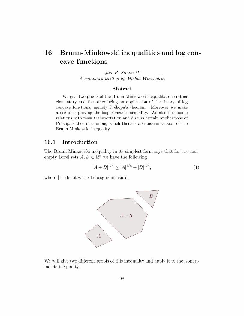
16 Brunn-Minkowski inequalities and log con-
cave functions
after B. Simon [1]A summary written by Micha l Warchalski
Abstract
We give two proofs of the Brunn-Minkowski inequality, one ratherelementary and the other being an application of the theory of logconcave functions, namely Prekopa’s theorem. Moreover we makea use of it proving the isoperimetric inequality. We also note somerelations with mass transportation and discuss certain applications ofPrekopa’s theorem, among which there is a Gaussian version of theBrunn-Minkowski inequality.
16.1 Introduction
The Brunn-Minkowski inequality in its simplest form says that for two non-empty Borel sets A,B ⊂ Rn we have the following
|A+B|1/n ≥ |A|1/n + |B|1/n, (1)
where | · | denotes the Lebesgue measure.
A
B
A+B
We will give two different proofs of this inequality and apply it to the isoperi-metric inequality.
98

The first proof will be rather elementary, initially showing the inequalityfor disjoint unions of rectangles via an induction argument and passing togeneral sets by approximation. We will also note an implicit connection ofthis proof with mass transportation. The second proof, on the other hand,follows from an application of a more general fact based on the theory of logconcave functions, namely Prekopa’s theorem. Hence, beforehand we willintroduce log concave functions and briefly look at their properties. More-over, we will discuss a Gaussian version of the Brunn-Minkowski inequalityas well as a kind of a counterpart of Prekopa’s theorem for measures givenby Gaussian densities.
First of all we note that we have another two equivalent formulations of(1). For two nonempty Borel sets A0, A1 ⊂ Rn and θ ∈ [0, 1] let
Aθ = θA0 + (1− θ)A1.
Proposition 1. The following statements are equivalent.
(i) For any two Borel sets A,B ⊂ Rn
|A+B|1/n ≥ |A|1/n + |B|1/n.
(ii) For any two Borel sets A0, A1 ⊂ Rn
|Aθ|1/n ≥ θ|A0|1/n + (1− θ)|A1|1/n. (2)
(iii) For any two Borel sets A0, A1 ⊂ Rn
|Aθ| ≥ |A0|θ|A1|1−θ. (3)
16.2 Application - the isoperimetric inequality
In this subsection we assume the Brunn-Minkowski inequality and apply itto the isoperimetric inequality. In particular, we will make a use of theformulation (3).
LetA(ε) = x : d(x,A) < ε,
where d(x,A) the denotes the distance of the point x from the set A. Givenan arbitrary measurable set A, we define its surface area by
s(A) := lim infε→0
|A(ε)| − |A|ε
.
99

In many cases, for example when A has smooth boundary, the above limitexists. We consider lim inf instead of lim sup, only because then the isoperi-metric inequality is stronger.
Theorem 2 (Isoperimetric inequality). Let A be a measurable set in Rn andlet B the open ball with the same volume as A. Then s(A) ≥ s(B).
Proof. By scaling we may assume that A has the same volume as the unitball B. Then we have
A(ε) = A+ εB = (1 + ε)
(1
1 + εA+
ε
1 + εB
)= (1 + ε)Aθ(ε),
with θ(ε) = ε/(1 + ε) and A0 = A, A1 = B.
ε
A(ε) = A+ εBA B
Applying the Brunn-Minkowski inequality (3) in this setting we obtain
|A(ε)| ≥ (1 + ε)n|B|.
substracting |A| = |B|, dividing by ε and passing to the lim inf on both sideswe obtain
s(A) ≥ n|B|.
This is exactly what we need, since
n|B| =ˆ 1
0
ˆSn−1
dΩ nrn−1dr = s(B).
100

16.3 The first proof
Here we will shortly sketch the first, more elementary, proof of the Brunn-Minkowski inequality (1).
Proof. As announced before, we proceed by induction, initially proving theresult for disjoint unions of rectangles with sides parallel to the coordinateaxes. If A is rectangle spanned by the sides a1, a2, ..., an and B is spanned bythe b1, b2, ..., bn, then A+B is spanned by the sides a1 +b1, a2 +b2, ..., an+bn.Then, by the geometric-arithemtic mean inequality we get
n∏j=1
c1/nj +
n∏j=1
d1/nj ≤ 1,
with cj = aj/(aj + bj) and dj = bj/(aj + bj), what is equivalent to theBrunn-Minkowski inequality in this case.
Next, we assume that A is a disjoint union of l rectangles and B is adisjoint union of m rectangles, with l +m ≥ 3. By disjointness, there existsa coordinate xi and a number α, such that the hyperplane xi = α separatesat least one pair of rectangles of A. This means that
A< = A ∩ x : xi < α,
A> = A ∩ x : xi > α,
are disjoint unions of at most l − 1 rectangles each.Now, by continuity of Lebesgue measure we can find a number β(α), such
that xi = β(α) separates the set B proportionally the same, so for
B< = B ∩ x : xi < β(α),
B> = B ∩ x : xi > β(α),
we have|B<||A<|
=|B>||A>|
=|B||A|
.
101

α β(α)
A< A> B< B>
“measure transportation”
This means that the function β(·) actually transports the probability measureν on the real line given by ν(−∞, t) = |B∩x : xi < t|/|B| to the probabilitymeasure µ defined as µ(−∞, t) = |A∩x : xi < t|/|A|. Using the last displayand that A<, B< and A>, B> are unions of at most l− 1 +m rectangles, theinduction gives
|A+B|disjointness
≥ |A< +B<|+ |A> +B>|induction
≥ (|A<|1/n + |B<|1/n)n + (|A>|1/n + |B>|1/n)n
the choice of β=
|A<||A|
(|A|1/n + |B|1/n)n +|A>||A|
(|A|1/n + |B|1/n)n
= (|A|1/n + |B|1/n)n.
16.4 The second proof
The second proof of (3) follows from a more general fact, however the argu-ment works for convex A0 and A1. It is based on the observation that if wedefine
C = (x, t) : 0 ≤ t ≤ 1, x ∈ tA0 + (1− t)A1 = At ⊂ Rn+1,
then the characteristic function of C for 0 ≤ θ ≤ 1 obeys the condition
χC(θ(x, t) + (1− θ)(y, s)) ≥ χC(x, t)θχC(y, s)1−θ (4)
102

(if we do this computation carefully, we use θA0 + (1 − θ)A0 ⊂ A0 andθA1 + (1 − θ)A1 ⊂ A1 for 0 ≤ θ ≤ 1 - that is why we need the convexityof A0 and A1). The Brunn-Minkowski inequality (3) says that an inequalitysimilar to the above holds also after integrating out χC in Rn
ˆχC(x, θ)dx = |Aθ|
≥ |A0|θ|A1|1−θ =
(ˆχC(x, 0)dx
)θ (ˆχC(x, 1)dx
)1−θ
Note that (4) roughly means, that logχC is concave. Functions of this kindwe call log concave.
Definition 3. A function f : Rn → [0,∞] is log concave if and only if it islower semicontinuous and for any x, y ∈ Rn, and 0 ≤ θ ≤ 1,
f(θx+ (1− θ)y) ≥ f(x)θf(y)1−θ.
The above considerations show that χC : Rn+1 → [0,∞] is log concaveand the Brunn-Minkowski inequality follows from Prekopa’s theorem.
Theorem 4 (Prekopa’s theorem). Let f be a log concave function on Rn+m,we write f(x, y) for x ∈ Rn and y ∈ Rm. Then the function g, defined as
g(y) :=
ˆRnf(x, y)dx
is a log concave function on Rm.
References
[1] Simon B., Convexity, Cambridge Univ. Press, Cambridge , 2011.
[2] Brascamp H. J., Lieb E. H., A logarithmic concavity theorem with someapplications, unpublished, 1974.
Micha l Warchalski, University of Bonnemail: [email protected]
103

17 Sharp fractional Hardy inequalities
after Rupert L. Frank and Robert Seiringer [?]A summary written by An Zhang
Abstract
The authors found a sharp fractional version of the Hardy inequal-ity, together with an explicit remainder term, which in particular alsorecovers the sharp Sobolev embedding into the Lorentz space. Theproof developed a nonlinear and nonlocal analogue of the classicalground state representation in a general setting.
17.1 Introduction
In this paper, we will study several Hardy inequalities, a generalization ofthe classical inequality on RN :
|∇u|p ≥ p−1|N − p||x−1u|p, (1)
which is an important object for study in analysis and mathematical physics.Extremizer (extremal function that make equality hold) for (1) doesn’t existin the corresponding homogeneous Sobolev space W 1,p for p > 1, while forp = 1, any symmetric decreasing function makes the inequality an equality.It’s then natural for people to consider sharp estimates for some fractionalinequalities of Hardy-type, both for (non)-local and (non)-linear cases, see[?, ?, ?] and reference there. Especially, Mazya-Shaposhnikova [?] got a nicebound (but not sharp) for the fractional Hardy (FH) inequality, which wasthere used to improve a Sobolev embedding estimate of Bourgain-Brezis-Mironescu [?]. Then a possible question is what’s the sharp constant for theFH inequality. Recently, Frank-Lieb [?] and then [?] got the sharp constantfor the FH inequality, respectively for linear-nonlocal and general nonlinear-nonlocal cases, with a ground state representation formula. The main newresult of [?] is the following theorem giving a sharp fractional Hardy inequal-ity for general exponent p ≥ 1 and fraction 0 < s < 1 with a remainderterm for p ≥ 2. The method is basically from nonlinear analysis, and somerearrangement will be needed to solve equality.
104

Theorem 1. Let N ≥ 1, 0 < s < 1, N/s 6= p ≥ 1, then for all u ∈ W s,p,5
¨RN×RN
|u(x)− u(y)|p
|x− y|N+psdxdy ≥ C
ˆRN
|u(x)|p
|x|psdx (2)
with the sharp constant
C = 2
ˆ 1
0
rps−1|1− r(N−ps)/p|pφ(r)dr,
where
φ(r) =
|SN−2|
´ 1
−1(1−t2)(N−3)/2dt
(1−2rt+r2)(N+ps)/2 , N ≥ 2
(1 + r)−(1+ps) + (1− r)−(1+ps), N = 1.
Extremizers for (2) don’t exist for p > 1 , while are all symmetric decreasingfunctions for p = 1. Moreover, if p ≥ 2, (2) has a remainder term
c
¨RN×RN
|v(x)− v(y)|pdxdy|x− y|N+ps(|x||y|)(N−ps)/2 , (3)
wherev = |x|(N−ps)/pu, c = min
τ∈(0,1/2)(1− τ)p − τ p + pτ p−1
Remark 2. 1. For simplicity, we fix C and c in this note. 2. The FHinequality (2) with remainder term (3) is an equality when p = 2 and c = 1,and the ground state representation for this special linear case has beengiven by [?]. The Fourier transform is a powerful tool in this case. 3.For nonlinear case, the core observation is that function ω = |x|(N−ps)/pis a critical point of the FH functional (2) but fails to lie in the handlingspace W s,p. It would be easier to see this from a local case in next subsec-tion. 4. A direct corollary is a sharp Sobolev embedding into Lorentz spaceW s,p → Lp
∗,p, p < N/s, p∗ = Np/(N − ps), and the fractional Sobolev es-timate of Bourgain-Brezis-Mironescu and Mazya-Shaposhnikova. The firstsharp estimate for Lorentz space is got from a rearrangement of Almgren-Lieb-type and the relation between the Lorentz norm and weighted Lp-norm.The second estimate comes from trivial Lorentz embedding.
5In default, we use the Sobolev space on RN for p < N/s, and RN \ 0 for p < N/s.
105

17.2 A general setting and examples
17.2.1 General setting
To generalize, we take a nonnegative symmetric measurable function k(x, y),consider the functional E[u] =
˜|u(x) − u(y)|pk(x, y), and if assume that
a ground state condition holds for a positive function ω and a real-valuedpotential V ,
2
ˆRN
(ω(x)− ω(y))|ω(x)− ω(y)|p−2k(x, y)dy = V (x)ω(x)p−1,
then we anticipate analogues of the sharp FH inequality, after setting u = ωv,
E[u]−ˆV |u|p ≥ c
¨|v(x)− v(y)|p(ω(x)ω(y))p/2k(x, y)dxdy χp≥2 (4)
To repair the possible diagonal singularity of the kernel, we give the followingprecise “virtual ground state condition”.
Condition 3. There exist positive measurable ω and a family of nonnegativesymmetric measurable functions (kε)ε>0(≤ k)→ k, ε→ 0, satisfying that
Vε = 2ω(x)−p+1
ˆRN
(ω(x)− ω(y))|ω(x)− ω(y)|p−2kε(x, y)dy
are absolutely convergent a.e., and have a weak limit V in L1loc.
Proposition 4. Under above condition, the general sharp FH inequality withremainder term, the representation formula (4) holds.
17.2.2 Examples
Linear case (p = 2).
1. pseudo-relativistic Schrodinger operators√−∆ +m2 + V0.
2. Schrodinger-type operator t(−i∇)+V0, where locally bounded function0 ≤ t . |x|2s for large x and some s ∈ (0, 1), and V0 ∈ LN/(2s) + L∞.
106

Intuition from a local case. Take E[u] =´g|∇u|p with a positive weight, then
if ω is the ground state of the energy functional I = E[u]−´V |u|p, that is
a positive weak solution of the corresponding weighted p-Laplace equation
−div(g|∇ω|p−2∇ω) = V ωp−1
then we have sharp FH inequality I ≥ 0.Proof. If we write u = wv, then from convexity inequality
|a+ b|p ≥ |a|p + p|a|p−2Rea · b, for any a, b ∈ CN , p ≥ 1,
and the p-Laplacian equation for ω, we get
E[u] =
ˆg|v∇ω + ω∇v|p
≥ˆg|v|p|∇ω|p + p
ˆg|∇ω|p−2ωRev|v|p−2∇v · ∇ω
=
ˆg|v|p|∇ω|p +
ˆg|∇ω|p−2ω∇(|v|p) · ∇ω
=
ˆg|v|p|∇ω|p −
ˆdiv(g|∇ω|p−2ω∇ω)|v|p
=
ˆg|v|p|∇ω|p −
ˆdiv(g|∇ω|p−2∇ω)ω|v|p −
ˆg|∇ω|p−2∆ω|v|p
=
ˆV |u|p.
From an enhanced convexity with remainder term c|b|p, we can get furthera remainder term I ≥ c
´gωp|∇v|p similarly. This is the well-known ground
state representation. In the special case g = 1, w = |x|(N−p)/p, we recoverthat for the classical inequality (1) uniformly.
17.3 Proof of the theorem
Using the idea from the proof for the local case in above subsection, proposi-tion 4 is trivial from the following lemma, using the ground state condition.
Lemma 5. Let p ≥ 1. For all t ∈ [0, 1], a ∈ C,
|a− t|p ≥ (1− t)p−1(|a|p − t).
107

For p > 1, the inequality is strict unless a = 1 or t = 0. Moreover, if p ≥ 2,then the inequality has a remainder term ctp/2|a− 1|p, which reaches equalityfor p = 2, while is strict unless a = 1 or t = 0 for p > 2.
Theorem 1 comes from proposition 4 and a lemma which checks theground state condition. From this condition, we can give two other formulasfor the sharp constant C after setting α = (N − ps)/p,
C = 2 limε→0
ˆ|ρ−1|>ε
dρsgn(ρα − 1)
|ρ− 1|2−p(1−s)∣∣∣1− ρ−α
1− ρ
∣∣∣p−1ρN−1(1− ρ)1+psφ(ρ), ρ < 1(1− ρ−1)1+psφ(ρ−1), ρ > 1,
=2|N − ps|p|SN−1|
¨|x|<1<|y|
||x|−α − |y|−α|p−1dxdy
|x− y|N+ps.
Sharpness of C. For p = 1, it’s trivial by inserting symmetric decreasingfunctions. For p > 1, extremizer doesn’t exist and to prove the sharpness ofC, we need to find a family of functions s.t. the quotient functional goes to C.Here we can choose, e.g. for N > ps, un = 1−n−α, |x| < 1; = |x|−α−n−α, 1 ≤|x| < n; = 0 otherwise.
References
[1] Michael Christ and Shuanglin Shao, Existence of extremals for a Fourierrestriction inequality, Anal. PDE 5 (2012), no. 2, 261–312. MR 2970708
[2] , On the extremizers of an adjoint Fourier restriction inequality,Adv. Math. 230 (2012), no. 3, 957–977. MR 2921167
[3] Damiano Foschi, Maximizers for the Strichartz inequality, J. Eur. Math.Soc. (JEMS) 9 (2007), no. 4, 739–774. MR 2341830 (2008k:35389)
[4] , Global maximizers for the sphere adjoint Fourier restriction in-equality, J. Funct. Anal. 268 (2015), no. 3, 690–702. MR 3292351
[5] Rene Quilodran, Nonexistence of extremals for the adjoint restriction in-equality on the hyperboloid, J. Anal. Math. 125 (2015), 37–70.
[6] E. M. Stein, Harmonic analysis: real-variable methods, orthogonality, andoscillatory integrals, vol. 43, Princeton University Press, 1993, With theassistance of T. S. Murphy, Monographs in Harmonic Analysis, III.
108
[7] E. M. Stein and G. Weiss, Introduction to Fourier analysis on Euclideanspaces, Princeton University Press, Princeton, N.J., 1971.
An Zhang, Peking University & University of Parisemail: [email protected], [email protected]
109

18 Optimal Young inequality: a symmetric
proof
after F. Barthe [2]A summary written by Pavel Zorin-Kranich
Abstract
We give a symmetric mass transport proof of the fact that Gaus-sians are extremizers of the Young convolution inequality in dimension1.
This summary answers a question that came up during the summerschool: is there a version of the mass transport argument from Barthe’sarticle [1] (presented by Johanna Richter) that is symmetric in the threefunctions in the dualized form of Young’s convolution inequality? This isindeed the case, and in fact even more general multilinear forms (appearingin Brascamp–Lieb inequalities) have been treated by this type of arguments,see [2]. Here we present a particularly simple instance in which the form isof convolution type and all functions are one-dimensional.
Theorem 1. Let n ≥ 2 and consider exponents 1 ≤ pi <∞, 1 ≤ i ≤ n, with∑i
1pi
= n − 1. Let also α ∈ Rn be given by αi = (p′i)−1/2, where p′i is the
Holder conjugate defined by 1pi
+ 1p′i
= 1. Then the form
Λ(~f) :=
ˆα⊥⊂Rn
⊗ni=1f1/pii
is maximized among the functions with ‖f1‖1 = · · · = ‖fn‖1 = 1 by theGaussians
Fi(x) =
√piπe−pix
2
.
The sharp Young convolution inequality can be recovered by a change ofvariables from the case n = 3. Unlike the proof in [1], our proof does notuse Holder’s inequality, and the above result in fact includes it as the specialcase n = 2 (again after a change of variables).
Proof. By standard truncation and approximation arguments we may restrictattention to strictly positive, smooth functions fi. In this case for each
110

i = 1, . . . , n there exists a unique monotonically increasing smooth mapui : R → R such that the pushforward measure (ui)]fi(x)dx coincides withFi(x)dx. This can be equivalently formulated as
fi · (u′i)−1 = Fi ui. (1)
Let now U := ⊗ni=1ui and let π : R → α⊥ denote the orthogonal projectiononto the hyperplane α⊥. Consider the change of variables π U : α⊥ → α⊥.Strict monotonicity of the ui’s and positivity of αi’s imply that this changeof variables is bijective.
The Jacobian J : α⊥ → α⊥ of this change of variables equals πU ′π.Writing U ′ : Rn → Rn in an orthogonal basis (α, ∗) we see that it has theform (
∗ ∗∗ J
).
Hence its (1, 1)-minor equals det J . On the other hand, by Cramer’s rule itequals detU times the (1, 1)-entry of (U ′)−1, which in turn equals 〈α, (U ′)−1α〉,since α is a unit vector by our scaling condition. Hence
det(J) =
∑ni=1 αi(u
′i)−1∏n
i=1(u′i)−1
.
The change of variables formula now gives
Λ(~f) =
ˆα⊥
⊗ni=1f1/pii
det(J) U−1 π−1
=
ˆα⊥
⊗ni=1(f1/pii (u′i)
−1)∑ni=1 αi(u
′i)−1 U−1 π−1
=
ˆα⊥
(⊗ni=1 F
1/pii π−1
)( ⊗ni=1(u′i)−1/p′i∑n
i=1 αi(u′i)−1 U−1 π−1
),
where we have used (1) in the last line. In the second tensor product weuse once again
∑ni=1
1p′i
= 1 and the arithmetic-geometric mean inequality to
estimaten∏i=1
(u′i)−1/p′i ≤
n∑i=1
αi(u′i)−1.
It follows that
Λ(~f) ≤ˆα⊥⊗ni=1F
1/pii π−1.
111

Now note that the function ⊗ni=1F1/pii equals a constant times a Gaussian, so
that⊗ni=1F
1/pii π−1 ≤ ⊗ni=1F
1/pii .
It follows that
Λ(~f) ≤ˆα⊥⊗ni=1F
1/pii = Λ(~F )
as claimed.
References
[1] Barthe, F. Optimal Young’s inequality and its converse: a simpleproof Geometric and Functional Analysis 8 (1998), pp. 234–242,arXiv:math/9704210.
[2] Barthe, F. On a reverse form of the Brascamp–Lieb inequality. Invent.Math. 134 (1998), pp. 335–361, arXiv:math/9705210.
Pavel Zorin-Kranich, University of Bonnemail: [email protected]
112