sharma chakravarthy - university of texas at arlington graph mining techniques and their...
TRANSCRIPT

1
Graph Mining Techniques and Their Applications
Sharma ChakravarthyInformation Technology Laboratory
Computer Science and Engineering DepartmentThe University of Texas at Arlington, Arlington, TX 76009
Email: [email protected]: http://itlab.uta.edu/sharma
Course URL: http://wweb.uta.edu/faculty/sharmac
© Sharma Chakravarthy 1
Acknowledgments
Parts of this presentation are based on the work of many of my students, especially Ramji Beera, Ramanathan Balachandran, Srihari Padmanabhan, Subhesh Pradhan (and others)
National Science Foundation and other agencies for their support of MavHome, Graph mining and other projects
Some slides are borrowed from various sources (web and others)
© Sharma Chakravarthy 2
Tutorial Outline
Graph Mining Approaches
Subdue
AGM
FSG
SQL‐Based Graph Mining
HDB‐Subdue
DB‐FSG (may be)
Graph mining applications
Email classification
Conclusions
References
© Sharma Chakravarthy 3
Need for Graph Mining
Association rule mining, decision trees and others mining approaches mine transactional data
Do not make use of any structural information
Graph based mining techniques are used for mining data that are structural in nature chemical compounds, complex proteins, VLSI
circuits, social networks, …
as mapping them to other representations is not possible or will lead to loss of structural information
© Sharma Chakravarthy 4

2
Need for Graph Mining Significant work in this area includes Subdue substructure discovery algorithm (Cook &
Holder),
HDB-Subdue (Chakrvarthy, Padmanabhan),
Apriori graph mining (AGM) (Inokuchi, Washio, and Motoda),
the frequent subgraph (FSG) technique (Karypis & Kuramochi), and
gSpan approach (J. Han), also SPIN (Huan, Wang, Prins, and Yang)
PageRank and HITS are also graph based
© Sharma Chakravarthy 5
Application:
To determine which amino acid chain dominates in a particular protein
Protein
Protein represented using Graph
O
N
H
NH
CN
C
COCO
© Sharma Chakravarthy 6
Application Domains
Chemical Reaction chains
CAD Circuit Analysis
Social Networks
Credit Domains
Web analysis
Games (Chess, Tic Tac toe)
Program Source Code analysis
Chinese Character data bases
Geology
Web and social network analysis
© Sharma Chakravarthy 7
Graph Based Data Mining
A Graph representation is an intuitive and an obvious choice for a database that has structural information
Graphs can be used to accurately model and represent scientific data sets. Graphs are suitable for capturing arbitrary relations between the various objects.
Graph based data mining aims at discovering interesting and repetitive patterns within these structural representations of data.
© Sharma Chakravarthy

3
Graph Mining: Mapping
Entities/objects Vertices
Object’s attributes Vertex label
Relations between Edges between verticesobjects
Type of relation edge label
Substructure Connected subgraph
Substructure Set of vertices & edges in
Instance input graph that match graph representation of data
© Sharma Chakravarthy 9
Graph Mining Overview
A substructure is a connected subgraph; need to differentiate between substructures and substructure instances
A connected subgraph is a subgraph of the original graph where there is a path between any two vertices
A subgraph Gs = (Vs, Es) of G = (V, E) is induced if Es contains all the edges of E that connect vertices in Vs
Directed and undirected edges are possible; multiple edges between two nodes need to be accommodated; cycles need to be handled
© Sharma Chakravarthy 10
Graph Mining: Complexity
Enumerating all the substructures of a graph has exponential complexity
Subgraph isomorphism (or subgraph matching) is NP‐complete
However, graph isomorphism although belongs to NP is neither known to be solvable in polynomial time nor NP‐complete
Generating canonical labels is O(|V|!), where V is the number of vertices
All approaches have to deal with the above in order to be able to work on large data sets
Different approaches do it differently; scalability depends on the approach and the use of representation
© Sharma Chakravarthy 11
Subdue
One of the earliest work in Graph based data mining Uses sparse adjacency matrix for graph representation
Substructures are evaluated using a metric called Minimum Description Length principle based on adjacency matrices
Capable of matching two graphs, differing by the number of vertices specified by the threshold parameter, inexactly
Performs hierarchical clustering by compressing the input graph with best substructure in each iteration
© Sharma Chakravarthy 12

4
Subdue
Capable of supervised discovery using positive and negative examples
Available main memory limits the largest dataset that can be handled
An SQL‐based subdue can address scalability
A computationally constrained beam‐search is used for subgraph generation
A branch and bound algorithm is used for inexact match
© Sharma Chakravarthy 13
AGM
First to propose apriori‐type algorithm for graph mining
Detects frequent induced subgraphs for a given support
Follows apriori algorithm
Not much optimization; hence performance is not that good and is not scalable!
© Sharma Chakravarthy 14
FSG
FSG is used for frequent subgraph discovery
Given a graph dataset G = {G1,G2,G3, ∙ ∙ ∙}, it discovers all connected subgraphs that are found in at least the support threshold percent of the input graphs
Uses a (sparse) adjacency matrix for graph representation
A canonical label is generated by flattening the adjacency matrix of a graph (optimization)
At each iteration FSG generates candidate subgraphs by adding one edge to the previous iteration’s frequent subgraph (optimization)
Graph isomorphism is checked by comparing canonical labels (optimization)
© Sharma Chakravarthy 15
gSpan
Avoids candidate generation
Builds a new lexicographical ordering among graphs and maps each graph to a unique minimum DFS code as its canonical label
Seems to outperform FSG
Amenable to parallelization
Does not handle cycles and multiple edges
© Sharma Chakravarthy 16

5
Subdue Example
object
triangle
R1
C1
T1
S1
T2
S2
T3
S3
T4
S4
Input Database Substructure S1(graph form)
Compressed Database
R1
C1
object
squareon
shape
shape S1 S1 S1
S1
• Came from AI• Examples are different from what we normally
see in mining
© Sharma Chakravarthy 17
SUBDUE : Overview
T1
T2 T3
S1
C1over
shape
shapeobject
object
triangle
square
over
shape
shapeobject
object
triangle
square
overshape
shapeobject
object
triangle
square
object
shape
object
circle
overover
overover
rectangle
shape
Best substructure output by Subdue
Substructure:
Graph(4v,3e):
v 1 object
v 2 object
v 3 triangle
v 4 square
u 1 2 over
u 1 3 shape
u 2 4 shape
© Sharma Chakravarthy 18
Subdue Substructure Discovery System
Subdue Substructure discovery system is a graph‐based data mining system that discovers interesting and repetitive patterns within graph representations of data.
It accepts as input a forest and identifies the substructure that best compresses the input graph using the minimum description length (MDL) principle.
It is capable of identifying both exact and inexact (isomorphic) substructures within a graph
It uses a branch and bound algorithm for inexact matches (substructures that vary slightly in their edge and vertex descriptions).
© Sharma Chakravarthy 19
Subdue
Unsupervised learning Subdue finds the most prevalent substructure from a set of unclassified input graphs
Supervised learning Subdue finds discriminating patterns from a set of classified (positive – G+ and negative – G‐ graphs)
Hierarchical conceptual clustering Compresses G with S and iterate
Incremental Subdue
© Sharma Chakravarthy 20

6
Subdue
Inferring graph grammars and graph primitives from examples
Applications
Data mining
Pattern recognition
Machine learning
© Sharma Chakravarthy 21
Graph Representation
Subdue represents data as labeled graph. Vertices represent objects or attributes Edges represent relationships between objects Input: Labeled graph Output: Discovered patterns and instances and
their compression. A substructure is a connected subgraph Graph isomorphism is used to identify similar (not
merely exact) substructures
© Sharma Chakravarthy 22
MDL Principle
Theory to minimize description length (DL) of data
information theoretic approach
Has been shown to be good across domains
Evaluates substructures based on their ability to compress DL of graph
Description length =DL(S) + DL(G/S) Depends upon the representation
Substructure that best compresses the original is chosen
© Sharma Chakravarthy 23
MDL Principle
Best theory: minimizes description length of data
Evaluate substructure based ability to compress DL of graph
Description length = DL(S) + DL(G|S)
© Sharma Chakravarthy 24

7
MDL Principle (cont.) Minimizes description length (DL) of data
Substructures are evaluated based on their ability to compress the
DL of the entire graph
MDL = description length of the compressed graph / description
length of the original graph
High MDL value is desirable !
DL(G) – Description length of the input graph
DL(S) – Description length of sub graph
DL(G|S) – Description length of the graph given the sub graph
DL(G)MDL =
DL(S) + DL(G|S)
© Sharma Chakravarthy 25
MDL
© Sharma Chakravarthy 26
vbits = Total number of bits to encode unique vertex labels
rbits = Total number of bits to encode adjacency matrix
ebits = Total number of bits to encode edge labels
I(G) = vbits + rbits + ebits
I(G)MDL = ‐‐‐‐‐‐‐‐‐‐‐‐‐‐‐‐‐‐‐‐‐‐‐‐‐‐
I(S) + I(G|S)
Subdue values substructures with high MDL as better substructures
MDL Details
© Sharma Chakravarthy 27
Example: Subdue
© Sharma Chakravarthy 28

8
Input (partial) The input is a file, with all the vertex labels, vertex
numbers, edges (using vertex numbers) and the edge directions
v 1 A
v 2 B
v 3 C
v 4 D
d 1 2 ab
d 1 3 ac
d 2 4 bd
d 4 3 dc
‘d’ stands for a directed edge and ‘u’ stands for undirected. ‘e’ stands for directed unless specified as undirected at the command prompt.
© Sharma Chakravarthy 29
Subdue Approach
Create a substructure for each unique vertex
Expand each substructure by adding an edge (and may be a vertex)
Maintain beam number of substructures for expansion
Halting conditions
Discovered substructures > limit
List maintaining the substructures to be expanded becomes empty
Max size of substructure to be discovered is reached
© Sharma Chakravarthy 30
Output
Output
Substructure: MDL value = 1.21789, instances = 2
Graph (4v,4e):
v 1 A
v 2 C
v 3 B
v 4 D
d 1 2 ac
d 1 3 ab
d 4 2 dc
d 3 4 bd
© Sharma Chakravarthy 31
Subdue Parameters
Threshold determines the amount of variation permissible in the vertex and edge descriptions during inexact graph match.
Nsubs determines the maximum number of substructures that are returned as the set of best substructures
Beam determines the maximum number of substructures that are retained for expansion in the next iteration of the discovery algorithm
Minsize constrains the size of substructures returned as best to be equal to or more than the specified parameter value
Limit is a upper bound on the number of substructures detected
© Sharma Chakravarthy 32

9
Subdue AlgorithmSubdue(Graph, BeamWidth, MaxBest, MaxSubSize, Limit)
ParentList = {}; ChildList = {}; BestList = {}
ProcessedSubs = 0
Create a substructure from each unique vertex label and its single‐vertex instances; insert the resulting
substructures in ParentList
while ProcessedSubs <= Limit and ParentList is not empty do
while ParentList is not empty do
Parent = RemoveHead(ParentList)
Extend each instance of Parent in all possible ways; Group the extended instances into Child substructures
foreach Child do
if SizeOf(Child) <= MaxSubSize then
Evaluate the Child //by using MDL
Insert Child in ChildList in order by value //highest to lowest MDL value
if Length(ChildList) > BeamWidth then Destroy the substructure at the end of ChildList
ProcessedSubs = ProcessedSubs + 1
Insert Parent in BestList in order by value
if Length(BestList) > MaxBest then Destroy the substructure at the end of BestList
Switch ParentList and ChildList
return BestList
© Sharma Chakravarthy 33
Algorithm (Contd.)
1. Create substructure for each unique vertex label
circle
rectangle
left
triangle
square
on
on
triangle
square
on
ontriangle
square
on
ontriangle
square
on
onleft
left left
left
Substructures:
triangle (4), square (4),circle (1), rectangle (1)
R1
C1
T1
S1
T2
S2
T3
S3
T4
S4object
triangle
object
squareon
shape
shape
R1
C1
S1 S1 S1
S1
© Sharma Chakravarthy 34
Algorithm (Contd.)
2. Expand best substructure by an edge or edge+neighboring vertex
circle
rectangle
left
triangle
square
on
on
triangle
square
on
ontriangle
square
on
ontriangle
square
on
onleft
left left
left
Substructures:
triangle
square
on
circleleftsquare
rectangle
square
on
rectangle
triangleon
R1
C1
T1
S1
T2
S2
T3
S3
T4
S4object
triangle
object
squareon
shape
shape
R1
C1
S1 S1 S1
S1
© Sharma Chakravarthy 35
Algorithm (cont.)
3. Keep only best substructures on queue (specified by beam width)
4. Terminate when queue is empty or #discovered substructures >= limit
5. Compress graph and repeat to generate hierarchical description
6. Constrained to run in polynomial time
R1
C1
T1
S1
T2
S2
T3
S3
T4
S4object
triangle
object
squareon
shape
shape
R1
C1
S1 S1 S1
S1
© Sharma Chakravarthy 36

10
Graph Match
Exact Graph match
Inexact Graph match
Exact graph match is likely to be restrictive for real life applications.
© Sharma Chakravarthy 37
Inexact Graph Match
Some variations may occur between instances
Want to abstract over minor differences
Difference = cost of transforming one graph to make it isomorphic to another
Match if cost/size < threshold
© Sharma Chakravarthy 38
Inexact Graph Match
Minimum graph edit distance
cumulative cost of graph changes required to transform the first graph into a graph isomorphic to the second graph.
Uses Branch and bound algorithm
© Sharma Chakravarthy 39
Graph 1
Graph 2
• Exact graph match is NP complete• Bunke and Allerman’s approach (1983, pattern recognition letters)
Each distortion is assigned a cost.A distortion is a basic transformation such as deletion, insertionof vertices and edges (and their labels)
Fuzzy graph match is a mapping f: N1 N2 U {λ}, N1 and N2 are sets of nodes of graph 1 and graph 2. A node v є N1 that is mapped to λ is deleted
• If matchcost <= threshold then two graphs are said to be isomorphic• Employing computational constraints such as bound on the number of
substructures considered makes subdue run in polynomial time
Mapping : 1 1, 2 2, 3 3, 4 null1) Delete Edge 3 4 (cost = 2) edge + label2) Delete vertex 4 (cost = 2) node + label3) Substitute vertex label C by D for vertex 3 (cost = 1)
Total cost = 5 for this mapping
© Sharma Chakravarthy 40

11
Costs
Cost of deleting (inserting) a node with a label a is given as DELNODE(a) (INSNODE(a))
Cost of substituting a node with syntactic label a by a node with syntactic label b are given by SUBNODE(a, b)
Similarly, SUBBRANCH(a, b) are costs of branch substitution
Branch deletion and insertion involves bordering nodes
DELBRANCH(a) (INSBRANCH(a)) and DELBRANCH’(A) (INSBRANCH’(A)) are used, respectively, when the border nodes are not deleted (or not inserted), and at least one of the border nodes are deleted (or inserted)
© Sharma Chakravarthy 41
Inexact match
Has three cases:
A node can be deleted
A node can be substituted, and
A node can be inserted
Mapping of nodes induces a mapping of branches, too. A branch is substituted/inserted/deleted when nodes are mapped
© Sharma Chakravarthy 42
Inexact match
DELNODE(x) = 2
SUBNODE(A, B) = SUBNODE(B, A) = 1
DELBRANCH(y) = 2
DELBRANCH’(y) = 1
INSBRANCH(y) = 2
F1: 2 4, 3 5, 1 Cost: 0 + 1 + 2 + 1 + 1 = 5
F2: 1 4, 2 5, 3 Cost: 1 + 1 + 2 + 1 + 1 = 6
4 5A Ba
3
1 2B Aa
a a
A
© Sharma Chakravarthy 43
Search space
(1,4) 1 (1,5) 0 (1,) 4
{(1,4),(2,5)}1+1
{(1,4),(2,)}1+4
{(1,5),(2,4)}0+4
{1,5),(2,)}4
{(1,),(2,5)}5
Least-cost match is {(1, ), (2,4), (3,5)}
4 5A Ba
3
1 2B Aa
a a
A
{(1,),(2,4)}4
{(1,4),(2,5),(3, )}1+1+4
{(1,),(2,4),(3,5)}5
© Sharma Chakravarthy 44

12
Variants of Subdue
Hierarchical reduction
Concept learner using positive and negative examples
Similarity detection in social networks
Inductive learning
Partitioned and parallel approaches
Database approach to some of the above
© Sharma Chakravarthy 45
Hierarchical Reduction Input is a labeled graph
A substructure is connected subgraph
A substructure instance is a subgraph isomorphic to substructure definition
Multiple iterations can create hierarchy
S1
S1
S1
S1
S1
S2
S2
S2
© Sharma Chakravarthy 46
Supervised Concept Learning Using Subdue
Need for non‐logic‐based relational concept learner
SubdueCL
Accept positive and negative graphs as input examples
Find hypotheses that describes positive examples and not negative examples
© Sharma Chakravarthy 47
SubdueCL
Find substructure compressing positive graphs, but not negative graphs
Find substructure covering positive graphs, but not negative graphs
Learn multiple rules
© Sharma Chakravarthy 48

13
Concept Learning Subdue
Positive graph G+, Negative graph G‐
Find substructure that compresses positive instances but not (or more than) negative instances
Value (G+, G‐, S) = DL(S) + DL(G+|S) + DL(G‐) – DL(G‐|S)
One of the limitations of this compression‐based concept learner is that it only looks for substructures which compress the entire positive graph more than the entire negative graph.
Therefore, it is biased to look for a substructure that offers more compression as compared to a substructure that covers a greater number of positive examples.
© Sharma Chakravarthy 49
Concept Learning SUBDUE
Positive graph G+
Negative graph G‐
Alternative set covering measure
Error (substructure) = #PosExNotCovered + #NegExCovered
#PosEx + #NegEx
For a substructure to be good, Error should be minimum
Hence, Value (of a substructure) = 1 ‐ Error
© Sharma Chakravarthy 50
Hypotheses detection using coverage
Main(Gp, Gn, Beam, Limit)
H = {};
repeat
repeat
BestSub = SubdueCL(Gp, Gn, Beam, Limit)
if BestSub = {}
then Beam m= Beam * 1.1
until (BestSub <> {})
Gp = Gp ‐ {p in Gp | BestSub covers p}
H = H + BestSub
until Gp = {}
return H
end
© Sharma Chakravarthy 51
SubdueCL Algorithm
SubdueCL(Gp, Gn, Limit, Beam)
ParentList = (All substructures of one vertex in Gp) mod Beam
repeat
BestList = {}
Exhausted = TRUE
i = Limit
while ( (i > 0 ) and (ParentList ≠ {}) )
ChildList = {}
foreach substucture in ParentList
C = Expand(Substructure)
if CoversOnePos(C,Gp)
then BestList = BestList ∪ {C}
ChildList = ( ChildList ∪ C ) mod Beam
i = i – 1
endfor
ParentList = ChildList mod Beam
endwhile
if BestList = {} and ParentList ≠ {}
then Exhausted = FALSE
Limit = Limit * 1.2
until ( Exhausted = TRUE )
return first(BestList)
end
© Sharma Chakravarthy 52

14
Example
object
object
object
on
on
triangle
square
shape
shape
© Sharma Chakravarthy 53
Empirical Results
Comparison with ILP (inductive logic programming) systems
Non‐relational domains from UCI repository
Subdue has also been extended for multiple classes
Golf Vote Diabetes Credit TicTacToe
FOIL 66.67 93.02 70.66 66.16 100.00
Progol 33.33 76.98 51.97 44.55 100.00
SubdueCL 66.67 94.88 64.21 71.52 100.00
© Sharma Chakravarthy 54
Graph‐based Anomaly Detection [KDD03] Anomalous substructure detection
Examine entire graph
Report unusual (low MDL compression) substructures
− low count
− lower MDL
− lower compression in subsequent passes
size * count can be used as a heuristic
© Sharma Chakravarthy 55
Graph‐based Anomaly Detection [KDD03] Anomalous subgraph detection
Partition graph into distinct, separate structures (subgraphs)
Determine how anomalous each subgraph is compared to others− How early compressed?
− How much compression?
© Sharma Chakravarthy 56

15
Graph Regularity
Regularity (predictability) affects degree of anomaly “In an insane society, the sane man appears insane”
Conditional Substructure Entropy: for substructures of a given size, how many bits are needed, on average, to describe the surroundings of the substructure?
© Sharma Chakravarthy 57
FSG
Aims at discovering interesting sub‐graph(s) thatappear frequently over the entire set of graphs incontrast to discovering a interesting sub‐graph(s)that appear within a single graph (or a forest) as inSubdue/HDB‐Subdue
It is designed along the lines of Apriori algorithm.
© Sharma Chakravarthy 58
Problem Definition
discovering all connected subgraphs that occurfrequently over the entire set of graphs.
Subdue: best n are output (n is user defined)
vertex : corresponds to an entity
edge : correspond to a relation between two entities
© Sharma Chakravarthy 59
Example of Frequent sub-graph discovery
© Sharma Chakravarthy 60

16
Definitions
Gs will be an induced subgraph of G if Vs is a subset of V and Es contains all the edges of E that connect vertices in Vs.
Two graphs G1 = (V1;E1) and G2 = (V2;E2) are isomorphic if they are topologically identical to each other, that is, there is a mapping from V1 to V2 such that each edge in E1 is mapped to a single edge in E2 and vice versa
An automorphism : an isomorphism mapping where G1 = G2 (on the same graph).
© Sharma Chakravarthy 61
Example (from wiki)
Graph G Graph HAn isomorphismbetween G and H
ƒ(a) = 1ƒ(b) = 6ƒ(c) = 8ƒ(d) = 3ƒ(g) = 5ƒ(h) = 2ƒ(i) = 4ƒ(j) = 7
• The two graphs shown below are isomorphic, despite their different looking drawings
• The formal notion of "isomorphism", e.g., of "graph isomorphism", captures the informal notion that some objects have "the same structure" if one ignores individual distinctions of "atomic" components of objects in question
© Sharma Chakravarthy 62
Canonical Labeling
“000000 1 01 011 0001 00010” “aaa z xy”
• Different orderings of the vertices will give rise to different codes• Try every possible permutation of the vertices and choose the ordering which
gives lexicographically the largest, or the smallest code.• O(|V|!)
© Sharma Chakravarthy 63
Canonical labeling
v2
a b
c
xv0 v1
y
V0 V1 V2
a b c
V0 a x y
V1 b
c2 c
abc xy
v2
c a
b
yv0 v1
x
V0 V1 V2
c a b
V0 c
V1 a y x
v2 b
cab yx
V1 V2 V0
a b c
V1 a x y
V2 b
v0 c
abc xy
© Sharma Chakravarthy 64

17
Definitions
The canonical label of a graph G = (V;E), cl(G) : unique code (e.g., string) that is invariant on the ordering of the vertices and edges in the graph.
Two graphs will have the same canonical label if they are isomorphic.
Canonical labels are useful to (i) compare two graphs (ii) establish a complete ordering of a set of graphs in a unique and and deterministic way, regardless of the original vertex and edge ordering.
© Sharma Chakravarthy 65
Key Features Of FSG
The complexity of finding a canonical labeling can, in practice, be substantially reduced by using the concept of vertex invariants
Introduces various optimizations for candidate generation and frequency counting
(Subdue has pruning, search space minimum detection etc.)
© Sharma Chakravarthy 66
Key Features Of FSG
Uses sparse graph representation that minimizes storage and computation (Subdue does the same)
Increases the size of frequent subgraphs by adding one edge at a time (apriori) (Subdue does the same)
Uses canonical labeling to uniquely identify subgraphs (Subdue uses bounded subgraph‐isomorphism with threshold as zero)
ONLY undirected edges; I believe it cannot handle multiple edges and cycles (Unlike subdue)
© Sharma Chakravarthy 67
FSG Components
Candidate Generation
Graph Isomorphism
Interestingness metric
Frequency is considered to be an interestingness metric. That is, the frequent sub‐graph that appears in most graph databases is considered interesting
© Sharma Chakravarthy 68

18
Graph Isomorphism
FSG uses canonical labeling for isomorphism.
Canonical labeling assigns a unique code for each substructure and two substructures have the same canonical code only if the substructures are isomorphic.
Canonical labeling is an easier and faster way of finding the isomorphic substructures, but it suffers from the fact that canonical labeling cannot be used for graphs that have multiple edges between the vertices and cycles
© Sharma Chakravarthy 69
Key Aspects
interested in subgraphs that are connected
allow the graphs to be labeled
both vertices and edges may have labels associated with them which are not required to be unique.
© Sharma Chakravarthy 70
FSG
Input to FSG Set of graphs (transactions) Labeled edges and vertices Edges are undirected No inexact match
Subdue can take a single connected graph or a forest of graphs
Edges can be directed or undirected Both edges and vertices can have labels Multiple edges between nodes is supported Cycles are supported
© Sharma Chakravarthy 71
Subdue ‐FSG
Subdue discovers conceptually interesting substructures in a single graph‐ FSG is used to discover subs‐graphs that occur frequently in a data set of graphs
The concept of Inexact graph match implemented by Subdue cannot be implemented by canonical labeling.
© Sharma Chakravarthy 72

19
Subdue‐FSG
Subdue requires to know the graph structure in the candidate generation phase but FSG does not need the adjacency list in the candidate generation phase, candidates are generated using the existing frequent substructures.
FSG prunes the candidate substructures using the ‘downward closure property’, which allows a k+1 size substructure to be a candidate only if all its k subs‐graphs are frequent substructures.
Grows Vs. generates
© Sharma Chakravarthy 73
Subdue ‐ FSG
Frequent subgraphs are found based on the set covering approach (frequency)
In Subdue subgraphs are found based on MDL (the graph that minimizes the description length of the input)
User defined support threshold – minimum percentage of graphs in which a subgraph has to be found
© Sharma Chakravarthy 74
Algorithm fsg(D; t)
1: F(1) = detect all frequent 1‐subgraphs in D2: F(2) = detect all frequent 2‐subgraphs in D3: k = 34: while F (k‐1) != NULL ; do5: C(k) = fsg‐gen(F(k‐1))6: for each candidate G(k) in C(k) do7: G(k).count = 08: for each transaction T in D do9: if candidate G(k) is included in transaction T then10: G(k).count++11: F(k) = {G(k) in C(k) | G(k).count >= t|D| }12: k++13: return F(1);F(2); ……… ;F(k‐2)
© Sharma Chakravarthy 75
Candidate generation
Candidates are the substructures which would be searched and counted in the given graph databases
create a set of candidates of size k+1, given frequent k‐subgraphs.
by joining two frequent k‐subgraphs (using downward closure property)
must contain the same (k‐1)‐subgraph (common core) Self‐join required for unlabeled graphs
Subdue extends subgraph in every possible way via an edge and a vertex
© Sharma Chakravarthy 76

20
Candidate generation
Unlike joining of two k‐itemsets which lead to a unique k_1‐itemset, the joining of two graphs of size k can lead to multiple distinct subgraphs of size k+1
1. Difference between the shared core and the two subgraphs can be a vertex that has the same label in both subgraphs
2. Core itself may have multiple automorphisms and each can lead to a different k+1 candidate (worst case k!)
3. Two frequent subgraphs may have multiple cores
© Sharma Chakravarthy 77
Joining of two k‐subgraphs
© Sharma Chakravarthy
Candidate Generation
© Sharma Chakravarthy 79
Join
© Sharma Chakravarthy 80

21
Key computational steps in candidate generation
core identification
Joining
using the downward closure property
© Sharma Chakravarthy 81
Core Identification
for each frequent k‐subgraph, store the canonical labels of its frequent (k‐1)‐subgraphs
Cores are the intersection of these lists. complexity : quadratic on |F(k)|
inverted indexing scheme for each frequent (k‐1)subgraph, maintain a list of child k‐subgraphs. form every possible pair from the child list of every (k‐1) frequent
subgraph. complexity of finding an appropriate pair of subgraphs: square of the
number of child k‐subgraphs (which is much smaller)
© Sharma Chakravarthy 82
Speeding automorphism computation
cache previous automorphisms associated with each core
look them up instead of performing the same automorphism computation again.
saved list of automorphisms is discarded once Ck+1 has been generated.
© Sharma Chakravarthy 83
Downward Closure
uses canonical labeling to substantially reduce the complexity of the checking whether or not a candidate pattern satisfies the downward closure property of the support condition
© Sharma Chakravarthy 84

22
Canonical labels
Canonical labels are computed for subgraphs
These labels are used for subgraph comparison (instead of isomorphism)
A number of optimizations are proposed to reduce the complexity from O(|V|!)
But once computed, they can be cached and used quickly for comparison
© Sharma Chakravarthy 85
Canonical Labeling
“000000 1 01 011 0001 00010” “aaa z xy”
• Different orderings of the vertices will give rise to different codes • Try every possible permutation of the vertices and choose the ordering which
gives lexicographically the largest, or the smallest code.• O(|V|!)
© Sharma Chakravarthy 86
Why canonical labeling?
use the canonical label repeatedly for comparison without the recalculation.
by regarding canonical labels as strings, we get the total order of graphs.
sort them in an array
index by binary search efficiently.
© Sharma Chakravarthy 87
Canonical label optimizations
Vertex invariants – do not change across isomorphism mappings (e.g., degree or label of a vertex)
Do not asymptotically change the computational complexity; in practicce it is useful
© Sharma Chakravarthy 88

23
Vertex Invariants
attributes or properties assigned to a vertex which do not change across isomorphism mappings.
partition the vertices into equivalence classes such that all the vertices assigned to the same partition have the same values for the vertex invariants.
only maximize over those permutations that keep the vertices in each partition together.
© Sharma Chakravarthy 89
Invariants degrees and labels of a vertex
Partition into disjoint groups
− Each partition has vertices with the same label and degree
the labels and degrees of their adjacent vertices (neighbor lists)
information about their adjacent partitions
© Sharma Chakravarthy 90
Vertex degree as invariant
only 1! * 2!= 2 permutations although the total permutations 4! = 24.
© Sharma Chakravarthy 91
Invariants degrees and labels of a vertex
Partition into disjoint groups
− Each partition has vertices with the same label and degree
the labels and degrees of their adjacent vertices (neighbor lists)
information about their adjacent partitions
© Sharma Chakravarthy 92

24
Neighbor lists
• (l(e); d(v); l(v)) •l(e) is the label of the incident edge e, •d(v) is degree of the adjacent vertex v, and •l(v) is its vertex label.
• same partition if and only if nl(u) = nl(v)
• reduce from 4! x 2! to 2! (1! * 2! * 1! * 1! * 1!).
© Sharma Chakravarthy 93
Invariants degrees and labels of a vertex
Partition into disjoint groups
− Each partition has vertices with the same label and degree
the labels and degrees of their adjacent vertices (neighbor lists)
Iterative partitioning (generalization of neighbor lists)
Use p(v) and l(e)
© Sharma Chakravarthy 94
Iterative Partitioningp(v): identifier of a partitionl(e): label of the incident edge to the neighbor vertex v
© Sharma Chakravarthy 95
Frequency Counting
for each frequent subgraph, keep a list of transaction identifiers that support it.
to compute the frequency of G(k+1), first compute the intersection of the TID lists of its frequent k‐subgraphs.
If the size of the intersection is below the support, G(k+1) is pruned ‐ subgraph isomorphism computations avoided
Otherwise use subgraph isomorphism on the set of transactions in the intersection of the TID lists.
© Sharma Chakravarthy 96

25
Chemical compound data set
More experimental results in the paper
© Sharma Chakravarthy 97
FSG vs. Subdue
No inexact graph matching
No iterative discovery
Restricts input in order to be more efficient
Undirected edges only
Set of disconnected graphs
Optimizations rely on additional space for increased speed
© Sharma Chakravarthy 98
Conclusions
Graph mining is a powerful approach needed by many real‐world applications
There is need for both Subdue class of mining algorithms and frequent subgraph class of algorithms
Scalability is an extremely important issue
Our approach to using SQL has yielded very promising scalability results (800K vertices and 1600K edges)
© Sharma Chakravarthy 99
Subdue FSG AGM gSpan HDBSubdue
Graph Mining
Multiple edges Hierarchical reduction
Cycles
Evaluation metric MDL Frequency Support, Confidence
Frequency DMDL
(frequency)
Inexact graph match
With threshold
Memory limitation
Comparison
© Sharma Chakravarthy 100
26
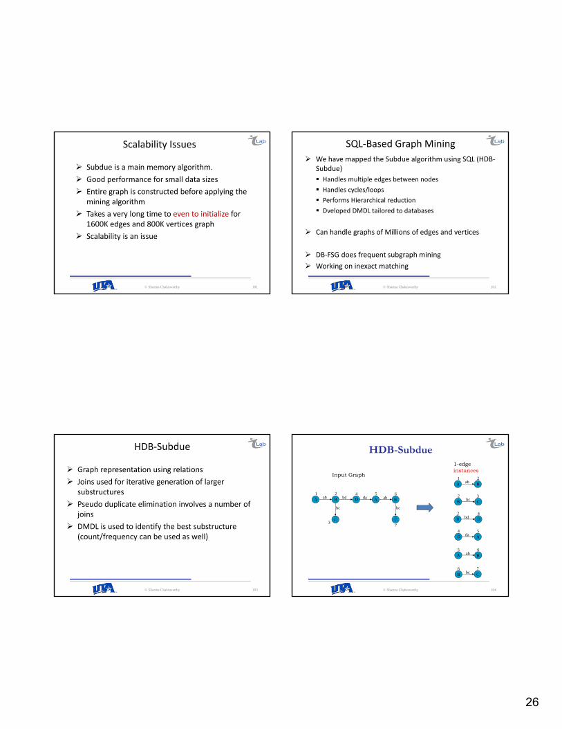
Scalability Issues
Subdue is a main memory algorithm.
Good performance for small data sizes
Entire graph is constructed before applying the mining algorithm
Takes a very long time to even to initialize for 1600K edges and 800K vertices graph
Scalability is an issue
© Sharma Chakravarthy 101
SQL‐Based Graph Mining
We have mapped the Subdue algorithm using SQL (HDB‐Subdue)
Handles multiple edges between nodes
Handles cycles/loops
Performs Hierarchical reduction
Dveloped DMDL tailored to databases
Can handle graphs of Millions of edges and vertices
DB‐FSG does frequent subgraph mining
Working on inexact matching
© Sharma Chakravarthy 102
HDB‐Subdue
Graph representation using relations
Joins used for iterative generation of larger substructures
Pseudo duplicate elimination involves a number of joins
DMDL is used to identify the best substructure (count/frequency can be used as well)
© Sharma Chakravarthy 103
A B
C
ab
bc
A B
C
bc
abD1 2 4 5
7
bd da6
3
A Bab1 2
B Cbc
2 3
B D2 4
bd
AD4 5
da
A Bab5 6
CB bc76
1-edge instances
Input Graph
HDB-Subdue
© Sharma Chakravarthy 104

27
1 edge pruning
A Bab 2
SubstructuresAfter pruning
B Cbc
2
A Bab1 2
B Cbc
2 3
B D2 4
bd
AD4 5
da
A Bab5 6
CB bc76
1 edge instances
A Bab 2
B Cbc
2
B Dbd1
AD da1
FrequentSubstructures
(count)
Group by
A Bab1 2
A Bab
5 6
B Cbc
2 3
CB bc76
Instances of Un-pruned substructures retained
© Sharma Chakravarthy 105
Generating 2 edge substructures
Instances of frequent substructures
BAab bc
C
1 2 3
BAab bc
C
5 6 7
A Bab1 2
B Cbc
2 3
BA ab5 6
CB bc76
1 edge instances
A Bab1 2
A Bab5 6
B Cbc
2 3
CB bc76
1-edge instances
BA ab bc C
1 2 3
BA ab bc C
5 6 7
2-edge instances
2BA ab bc C
Frequent 2-edge Substructures (count)
Group by
© Sharma Chakravarthy 106
Representing input graph using relations
Input stored in two tables
vertexno vertexlabel
1 A
vertex1 vertex2 edgename
1 2 ab
Vertices
Edges
© Sharma Chakravarthy 107
The pseudo code of HDB‐SubdueINPUT : (Input graph flat file, MaxSize, Beam, NumberOfIterations)BEGIN HDB‐SubdueLoad vertices and edges from flat file into relations;Remove the edges which have only one instance from the edge tableFor (i=1 to NumberOfIterations) { // For Hierarchical reductionFor (j=2 to MaxSize) { // Substructure expansionJoin instance_(j‐1) with oneedge table to generate instance_jEliminate pseudo duplicates from instance_j tableGroup instance_j by vertex label and edge label to obtain substructures and its
countCalculate DMDL for substructures and insert them into sub_fold_j tableRetain top Beam substructures in sub_fold_j table and remove the rest
Retain only the instances of sub_fold_j table in instance_j table and eliminate others}‐‐‐ End of iteration i ‐‐‐Select the best substructure of iteration iCompress the substructure by updating vertex table and oneedge table}
End HDB‐Subdue
© Sharma Chakravarthy 108
28
3
A B
C
ab
bc
A B
C
bc
abD
1 2 4 5
7
bd da6
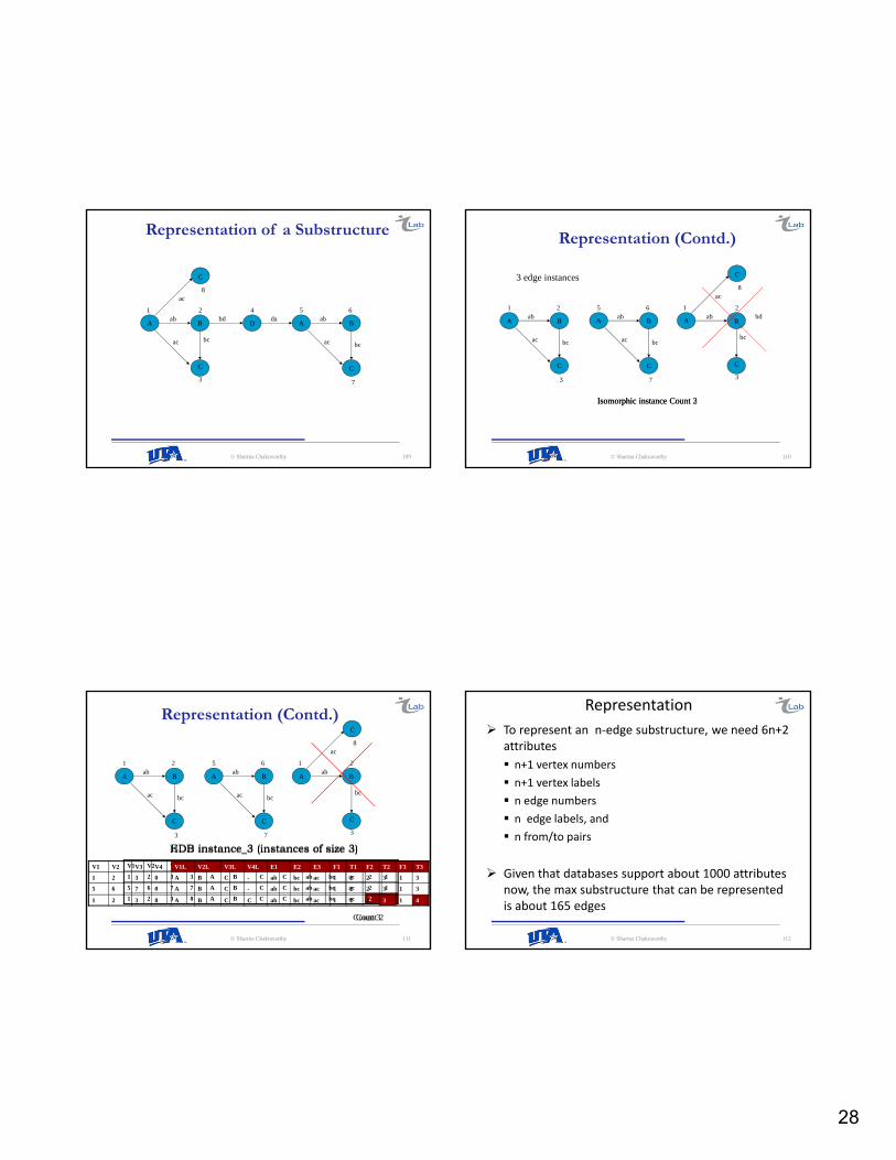
Representation of a Substructure
8
C
ac ac
ac
© Sharma Chakravarthy 109
A B
C
bc
ab5
7
6
ac
A B
C
bc
ab1
3
2
ac
3
A B
C
ab
bc
1 2bd
8
C
ac
Isomorphic instance Count 3Isomorphic instance Count 2
Representation (Contd.)
3 edge instances
© Sharma Chakravarthy 110
A B
C
bc
ab5
7
6
ac
A B
C
bc
ab1
3
2
ac
3
A B
C
ab
bc
1 2
8
C
ac
EDB instance_3 (instances of size 3)
V1 V2 V3 V4 V1L V2L V3L V4L E1 E2 E3 X1 X2
1 2 3 3 A B C C ab bc ac 2 1
5 6 7 7 A B C C ab bc ac 2 1
1 2 3 8 A B C C ab bc ac 2 1
V1 V2 V3 V4 V1L V2L V3L V4L E1 E2 E3 F1 T1 F2 T2 F3 T3
1 2 3 0 A B C - ab bc ac 1 2 2 3 1 3
5 6 7 0 A B C - ab bc ac 1 2 2 3 1 3
1 2 3 8 A B C C ab bc ac 1 2 2 3 1 4
Count 2Count 3
Representation (Contd.)
HDB instance_3 (instances of size 3)
© Sharma Chakravarthy 111
Representation
To represent an n‐edge substructure, we need 6n+2 attributes
n+1 vertex numbers
n+1 vertex labels
n edge numbers
n edge labels, and
n from/to pairs
Given that databases support about 1000 attributes now, the max substructure that can be represented is about 165 edges
© Sharma Chakravarthy 112

29
3
A B
C
ab
bc
A B
C
bc
abD
1 2 4 5
7
bd da6
ab
vertex1 vertex2 edge1 vertex1name vertex2name
1 2 ab A B
1 2 ab A B
1 2 ab A B
. . . . .
vertex1 vertex2 edge No edge1 vertex1name vertex2name
1 2 1 ab A B
1 2 2 ab A B
1 2 3 ab A B
. . . . . .
EDB-Oneedge table
HDB-Oneedge table
Need for Edge numbersab
© Sharma Chakravarthy 113
INSERT INTO instance_n( SELECT i.vertex1 .. i.vertex(n), o.vertex2, i.vertex1name .. i.vertex(n)name,
o.vertex2name, i.edge1 .. i.edge(n), o.edge, i.ext1 , 1 FROM instance(n-1) i, oneedge oWHERE i.vertex(k) = o.vertex1 and i.vertex(k+1) < o.vertex2 and .. i.vertex(n) <
o.vertex2)
3
A B
C
2 ab
4 bc
A B
C
8 bc
7 abD
1 2 4 5
7
5 bd 6 da6
1 ab
3 ab
Constrained Expansion
© Sharma Chakravarthy 114
A B2 ab
1 21 ab
A B
1 21 ab
Instance_1 table
A B2 ab
1 2
HDB-Oneedge table
WHERE i.vertex1 = o.vertex1
Instance_1 table
=
.
2
edgeNo
.....
BAab21
vertex2namevertex1nameedgevertex2vertex1HDB-Oneedge table
.
1
edge1No
.....
B
vertex2name
A
vertex1name
ab
edge1
21
vertex2vertex1
WHERE i.vertex1 = o.vertex1 and o.edgeNo <> i.edge1No
<>
Unconstrained expansion
© Sharma Chakravarthy 115
Expansion
To expand a 1‐edge substructure with 2 vertices V1 and V2, we need to:
expand self‐edges on V1 or V2 (in general n)
expand multiple edge from v2 to v1 (or n*(n‐1))
expand incoming edge on V1 or V2 (or n)
expand outgoing edge on V1 or V2 (or n)
In general, to expand a substructure of size n, we need n**2 + 2n queries
These queries are generated (can be one union query)
If you know that multiple edges and/or cycles do not exist, less number of queries can be used
© Sharma Chakravarthy 116

30
Expansion VL1 VL2 VL3 EL1 EL2 F1 T1 F2 T2 COUNT DMDL
A B C AB AC 1 2 1 3 3 1.8
A B D AB BD 1 2 2 3 1 0.9
B D A BD DA 1 2 2 3 1 0.9
D A B DA AB 1 2 2 3 1 0.9
D A C DA AC 1 2 2 3 1 0.9
© Sharma Chakravarthy 117
ab bc bcabcd da3
A
1 2 4 5 76
B C D A B C E A
B
C F A C G
B
8 9
10
11 12 13
14
15 16ce ea ac
ab
cf fa ac
ab
cg
Substructure Evaluation metric
Example
2 Edge substructure instances
© Sharma Chakravarthy 118
Subdue MDL
A B
C
ab9 11
10
ac
0 1 1
0 0 0
0 0 0
0 1 0
0 0 1
0 0 0
1 2 3
1
2
3
Count = 2 Count = 2
BAab
1 2C3
bc
MDL = 1.14539 MDL = 1.12849
DL(G)MDL =
DL(S) + DL(G|S)
9
10
11
9 10 11
Adjacency matrix Adjacency matrix
© Sharma Chakravarthy 119
A B
C
ab9 11
10
ac
count = 2sub_vertices = 3non-zero rows = 1
BAab
1 2C3
bc
• Value(G) = graph_vertices + graph_edges
• Value(S) = sub_vertices + non-zero rows
• Value(G|S) = (graph_vertices – sub_vertices * count + count) + (graph_edges –sub_edges * count)
Value (G)
Value (S) + Value (G|S)DMDL =
0 1 1
0 0 0
0 0 0
9 10 11
9
10
11
0 1 0
0 0 1
0 0 0
1 2 3
1
2
3
DMDL = 1.1481 DMDL = 1.1071
DMDL
count = 2sub_vertices = 3non-zero rows = 2
© Sharma Chakravarthy 120

31
A Bab9 11
ab
ac
EDB – Subdue:
No of vertices = No of edges + 1
No of vertices = 3 + 1 = 4
V1 V2 V3 V4 V1L V2L V3L V4L E1 E2 E3 F1 T1 F2 T2 F3 T3
9 11 10 0 A B - - AB AB AC 1 2 1 2 1 3
. . . . . . . . . . . . . . . . .
Repeating vertex marked by vertex invariant (0’s and –’s)
No of vertices = count of non zero vertex numbers = 3
OR
No of vertices = count of unique connectivity attributes = 3
C 10
sub_vertices
Three edge
Instance_3 table
© Sharma Chakravarthy 121
A Bab9 11
ab
ac
C 10
0 1 1
0 0 0
0 0 0
9 10 11
9
10
11
Non Zero Rows = 1
V1 V2 V3 V3 V1L V2L V3L V3L E1 E2 E3 F1 T1 F2 T2 F3 T3
9 11 10 0 A B - - ab ab ac 1 2 1 2 1 3
. . . . . . . . . . . . . . . . .
• Non zero row in adjacency matrix will have out degree of at least 1
• The Fn attribute represents outgoing vertex
• Count of unique Fn attributes gives number of non-zero rows
non-zero rows
Adjacency matrix
Three edge
Instance_3 table
© Sharma Chakravarthy 122
A Bab9 11
ab
ac
C 10
• Value(G|S) = (graph_vertices – sub_vertices * count + count) + (graph_edges – sub_edges * count)
= (3 – 3*2 + 2) + (3 – 2*2) = -2= (3 – 3*1 + 1) + (3 – 2*1) = 2
• Tells how many vertices of the entire graph, the substructure can compress
• Both the instances remove same set of vertices, therefore count = 1
count
A Bab9 11
ac
C 10
A B
9 11ab
ac
C 10
Count = 2
Two edge substructure instances
© Sharma Chakravarthy 123
V1 V2 V3 V1L V2L V3L E1 E2 F1 T1 F2 T2
9 11 10 A B C ab ac 1 2 1 3
9 11 10 A B C ab ac 1 2 1 3
. . . . . . . . . . . .
• GROUP BY vertex, edge label and connectivity attributes gives count of all instances, i.e. 2
• GROUP BY vertex number, within instances of a particular substructure will return group of instances containing unique vertex numbers
• Count on the number of such groups gives the updated count of instances. In this case it is 1
• Therefore Instead of counting 2, we count as 1
Count = 21 Group with 2 instances
Count = 1
V1 V2 V3 V1L V2L V3L E1 E2 F1 T1 F2 T2
9 11 10 A B C ab ac 1 2 1 3
. . . . . . . . . . . .
count (Contd..)Instance_2 table
© Sharma Chakravarthy 124

32
3
A B
C
ab
bc
A B
C
bc
abD
1 2 4 5
7
bd da6
3
C
bc
A Bab
1 2
A Bab
1 2
3
B Cbc
2
Aab
1
3
B
C
bc
2
One edge instancesTwo edge
instances
Pseudo duplicates
© Sharma Chakravarthy 125
V1 V2 V3 V1L V2L V3L E1 E2 F1 T1 F2 T2
1 2 3 A B C AB BC 1 2 2 3
2 3 1 B C A BC AB 1 2 3 1
. . . . . . . . . . . .
3
C
bc
A Bab
1 2
Aab
1
3
B
C
bc
2
Instance_2 table
V1 V2 V3 V1L V2L V3L E1 E2 F1 T1 F2 T2
1 2 3 A B C AB BC 1 2 2 3
1 2 3 A B C AB BC 1 2 2 3
. . . . . . . . . . . .
Pseudo duplicates (Contd..)
Two edge
© Sharma Chakravarthy 126
In SQL, only rows can be sorted
Tasks:
• Convert columns into rows
• Sort the rows
• Convert rows into columns
V1 V2 V3 V1L V2L V3L E1 E2 F1 T1 F2 T2
2 3 1 B C A BC AB 1 2 3 1
. . . . . . . . . . . .
Instance_2 table
Unsorted_VUnsorted_E
V VL POS
2 B 1
3 C 2
1 A 3
. . .
E F T
BC 1 2
AB 3 1
. . .
Pseudo duplicates (Contd..)
© Sharma Chakravarthy 127
Unsorted_V
V VL POS
2 B 1
3 C 2
1 A 3
. . .
Unsorted_E
E F T
BC 1 2
AB 3 1
. . .
Sort on V
Sorted_V
32C3
.
1
3
POS
...
2B2
1A1
NEW POSVLV
Sorted_V
32C3
.
1
3
POS
...
2B2
1A1
NEW POSVLV
Sorted_V
32C3
.
1
3
POS
...
2B2
1A1
NEW POSVLV
Updated_E
E F T
BC 2 3
AB 1 2
. . .
Sorted_E
E F T
AB 1 2
BC 2 3
. . .
Sort on F, T
3 Way Join
Updating connectivity attributes
© Sharma Chakravarthy 128
33
Sorted_V
32C3
.
1
3
POS
...
2B2
1A1
NEW POSVLV
Sorted_V
32C3
.
1
3
POS
...
2B2
1A1
NEW POSVLV
Sorted_V
32C3
.
1
3
POS
...
2B2
1A1
NEW POSVLV
V1 V2 V3 V1L V2L V3L E1 E2 F1 T1 F2 T2
1 2 3 A B C AB BC 1 2 2 3
. . . . . . . . . . . .
Instance_2 table
Sorted_E
E F T
AB 1 2
BC 2 3
. . .
Sorted_E
E F T
AB 1 2
BC 2 3
. . .
2n+1 Way Join for reconstruction
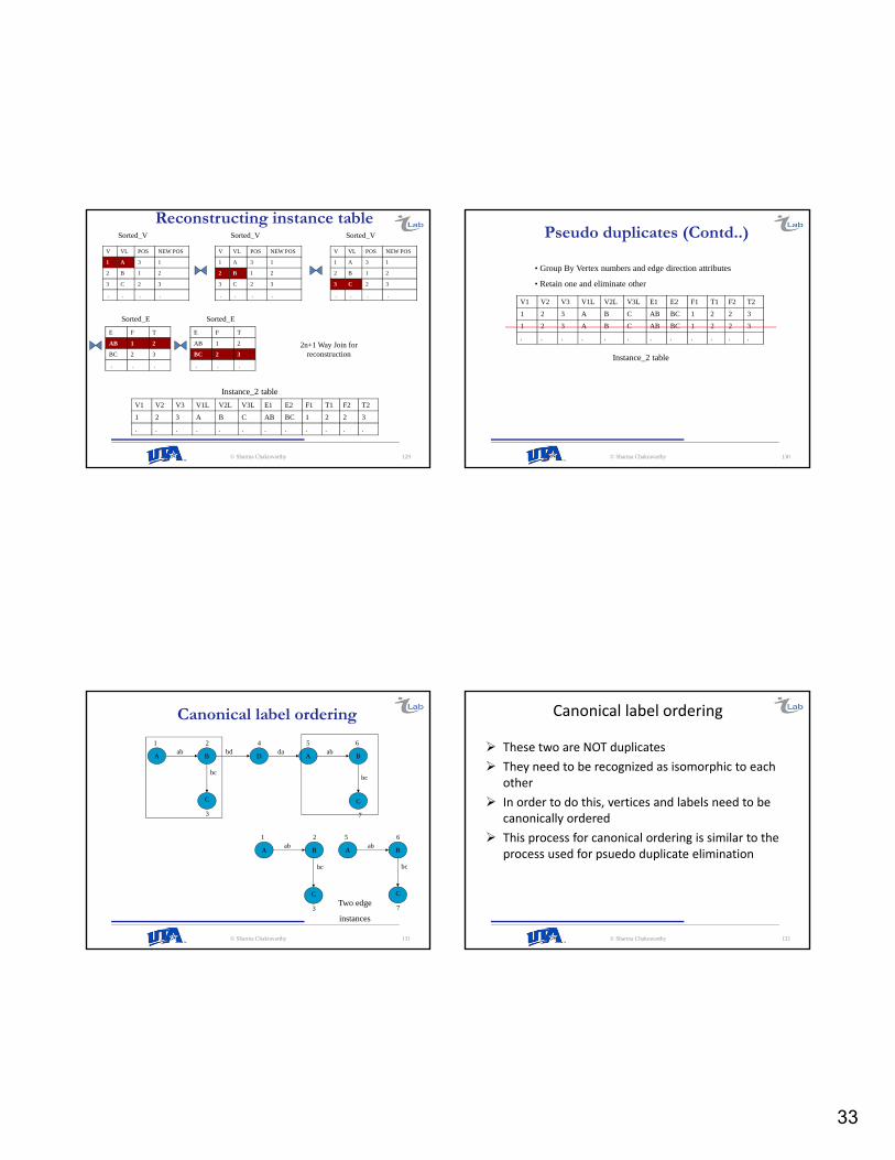
Reconstructing instance table
© Sharma Chakravarthy 129
V1 V2 V3 V1L V2L V3L E1 E2 F1 T1 F2 T2
1 2 3 A B C AB BC 1 2 2 3
1 2 3 A B C AB BC 1 2 2 3
. . . . . . . . . . . .
• Group By Vertex numbers and edge direction attributes
• Retain one and eliminate other
Pseudo duplicates (Contd..)
Instance_2 table
© Sharma Chakravarthy 130
3
A B
C
ab
bc
A B
C
bc
abD
1 2 4 5
7
bd da6
3
C
bc
A Bab
1 2
Aab
5
7
B
C
bc
6
Two edge
instances
Canonical label ordering
© Sharma Chakravarthy 131
Canonical label ordering
These two are NOT duplicates
They need to be recognized as isomorphic to each other
In order to do this, vertices and labels need to be canonically ordered
This process for canonical ordering is similar to the process used for psuedo duplicate elimination
© Sharma Chakravarthy 132

34
3
A B
C
ab
bc
A B
C
bc
abD
1 2 4 5
7
bd da6
3
C
bc
A Bab
1 2ab
3
B
C
bc
2
ca
ca
A
1
ca
Cycles – Marking repeated vertex
Three edge starting with ab Three edge starting with bc
© Sharma Chakravarthy 133
V1 V2 V3 V4 V1L V2L V3L V4L E1 E2 E3 F1 T1 F2 T2 F3 T3
1 2 3 1 A B C A AB BC CA 1 2 2 3 3 4
2 3 1 2 B C A B BC CA AB 1 2 2 3 3 4
V1 V2 V3 V4 V1L V2L V3L V4L E1 E2 E3 F1 T1 F2 T2 F3 T3
0 1 2 3 - A B C AB BC CA 2 3 3 4 4 2
0 1 2 3 - A B C AB BC CA 2 3 3 4 4 2
3
C
bc
A Bab
1 2
ca
V1 V2 V3 V4 V1L V2L V3L V4L E1 E2 E3 F1 T1 F2 T2 F3 T3
1 2 3 0 A B C - AB BC CA 1 2 2 3 3 1
2 3 1 0 B C A - BC CA AB 1 2 2 3 3 1
Instance_3 table
Cycles – Marking repeated vertex (Contd..)
Instance_3 table with vertex invariants 0’s and –’s
© Sharma Chakravarthy 134
Hierarchical Reduction
D
3 AB
2 A
B C3 4
4 AC 5 AB
5A
B C6 7
6 AC
1
1 DA 2 DA
3 AB
2 A
B C3 4
4 AC 5 AB
5A
B C6 7
6 AC
ABA
B CAC
Best substructure
Best substructure instances
Input graph
© Sharma Chakravarthy 135
Hierarchical Reduction (Contd..)
D
3 AB
2 A
B C3 4
4 AC 5 AB
5A
B C6 7
6 AC
1
1 DA 2 DA
SUB_18 SUB_1 9
ABA
B C
AC SUB_1
Input graph
Best substructure Compressing vertex
© Sharma Chakravarthy 136

35
Hierarchical Reduction (Contd..)
Tasks in Hierarchical Reduction:
1. Select the best substructure after each iteration
2. Identify the instances of the best substructure
3. For each instance
(1) Remove the vertices from the input graph
(2) For every instance removed include a new vertex to the input graph
(3) Remove the edges from the input graph
(4) Update the vertex number of the edges that are incident on or going out of the compressed instance
4. The compressed input graph participates in the next iteration
© Sharma Chakravarthy 137
Selecting the best substructure
3
D
3 AB2 A
B C4
4 AC 5 AB5 A
B C6 7
6 AC
11 DA 2 DA
subfold_2
V1L V2L V3L E1 E2 F1 T1 F2 T2 COUNT DMDL
A B C AB AC 1 2 1 3 2 1.71
D A B DA AB 1 2 2 3 2 1.34
D A C DA AC 1 2 2 3 2 1.34
D A A DA DA 1 2 1 3 1 0.75
Best substructure is one with highest DMDL value
© Sharma Chakravarthy 138
Identify instances of best substructure
V1 V2 V3 V1L V2L V3L E1N E2N E1 E2 F1 T1 F2 T2 DMDL
2 3 4 A B C 3 4 AB AC 1 2 1 3 1.71
5 6 7 A B C 5 6 AB AC 1 2 1 3 1.71
BestInstances
3
D
3 AB2 A
B C4
4 AC 5 AB5 A
B C6 7
6 AC
11 DA 2 DA
© Sharma Chakravarthy 139
Updating vertex table
V1 V2 V3 V1L V2L V3L E1N E2N E1 E2 F1 T1 F2 T2 DMDL
2 3 4 A B C 3 4 AB AC 1 2 1 3 1.71
5 6 7 A B C 5 6 AB AC 1 2 1 3 1.71
BestInstances
V VL
1 D
2 A
3 B
4 C
5 A
6 B
7 C
DELETE FROM VertexTableWHERE VertexNo IN (
(SELECT V1 FROM BestInstances)UNION (SELECT V2 FROM BestInstances)
. . . .UNION (SELECT Vn+1 FROM BestInstances))
Vertex table
D
3 AB 4 AC 5 AB 6 AC
11 DA 2 DA
V VL
1 D
8 SUB_1
9 SUB_1
3
D
3 AB2 A
B C4
4 AC 5 AB5 A
B C6 7
6 AC
11 DA 2 DA
1D
3 AB 4 AC 5 AB 6 AC
1 DA 2 DA
8 9SUB_1 SUB_1
© Sharma Chakravarthy 140

36
Updating oneedge table
V1 V2 V3 V1L V2L V3L E1N E2N E1 E2 F1 T1 F2 T2 DMDL
2 3 4 A B C 3 4 AB AC 1 2 1 3 1.71
5 6 7 A B C 5 6 AB AC 1 2 1 3 1.71
BestInstances
EL EN V1L V2L V1 V2
DA 1 D A 1 2
DA 2 D A 1 5
AB 3 A B 2 3
AC 4 A C 2 4
AB 5 A B 5 6
AC 6 A C 5 7
Oneedge table
DELETE FROM oneedgeWHERE EdgeNo IN (
(SELECT E1N FROM BestInstances)UNION (SELECT E2N FROM BestInstances)
. . . .UNION (SELECT EnN FROM BestInstances))
EL EN V1L V2L V1 V2
DA 1 D SUB_1 1 8
DA 2 D SUB_1 1 9
UPDATE oneedge set V1=MAX_VERTEXWHERE V1 IN (
(SELECT V1 FROM BestInstances WHERE rownum = 1). . . .
UNION (SELECT Vn+1 FROM BestInstances WHERE rownum = 1))
UPDATE oneedge set V2=MAX_VERTEXWHERE V2 IN (
(SELECT V1 FROM BestInstances WHERE rownum = 1). . . .
UNION (SELECT Vn+1 FROM BestInstances WHERE rownum = 1))
1
D
3 AB 4 AC 5 AB 6 AC
1 DA 2 DA
8 9SUB_1 SUB_1
1
D1 DA 2 DA
8 9SUB_1 SUB_1
1
D1 DA 2 DA
8 9 SUB_1SUB_1 3
D
3 AB2 A
B C4
4 AC 5 AB5 A
B C6 7
6 AC
11 DA 2 DA
© Sharma Chakravarthy 141
Experimental Results
Setup: Input graphs generated using the graph generator developed by AI Lab Platform: Linux Database: Oracle 10g Machine’s memory: 2 Gbytes Number of processors: 2
Graph GeneratorInput: Specs of subs to
be embedded
Subdue.g file
SQL Loader
Vertex TableEdge Table
CSV Converter.g file
Thanks to AI Lab for the synthetic generator
© Sharma Chakravarthy 142
No cycles and multiple edges
Dataset Instances50V100E 4250V500E 15500V1000E 301KV2KE 602.5KV5KE 1505KV10KE 3007.5KV15KE 45010KV20KE 60015KV30KE 90020KV40KE 120050KV100KE 3000100KV200KE 6000200KV400KE 12000400KV800KE 24000800KV1600KE 48000
© Sharma Chakravarthy 143
No cycles and multiple edges
• Running time grows exponentially with graph input size• Subdue crossover – 2.5KV5KE
Beam 4, MaxSize 5, Iterations 1
0.1
1
10
100
1000
10000
100000
1000000
50V100E
250V500E
500V1000E
1KV2KE
2.5KV5KE
5KV10KE
7.5KV15KE
10KV20KE
15KV30KE
20KV40KE
50KV100KE
100KV200KE
200KV400KE
400KV800KE
800KV1600KE
Dataset
Tim
e in
se
co
nd
s
Subdue
HDB-Subdue
EDB-Subdue
© Sharma Chakravarthy 144

37
With cycles and multiple edgesDataset Instances50V100E 4250V500E 15500V1000E 301KV2KE 602.5KV5KE 1505KV10KE 3007.5KV15KE 45010KV20KE 60015KV30KE 90020KV40KE 120050KV100KE 3000100KV200KE 6000200KV400KE 12000400KV800KE 24000800KV1600KE 48000
© Sharma Chakravarthy 145
With cycles and multiple edges
• Subdue crossover – 2.5KV5KE
Beam 4, MaxSize 5, Iterations 1
0.010.1
110
1001000
10000100000
1000000
50V1
00E
250V
500E
500V
1000
E
1KV2
KE
2.5KV
5KE
5KV1
0KE
7.5KV
15KE
10KV
20KE
15KV
30KE
20KV
40KE
50KV
100K
E
100K
V200
KE
200K
V400
KE
400K
V800
KE
800K
V160
0KE
Dataset
Tim
e in
se
co
nd
s
Subdue HDB-Subdue
© Sharma Chakravarthy 146
Hierarchical ReductionDataset Instances50V100E 2250V500E 10500V1000E 201KV2KE 402.5KV5KE 805KV10KE 1607.5KV15KE 25010KV20KE 32015KV30KE 42020KV40KE 64050KV100KE 1280100KV200KE 2560200KV400KE 5120400KV800KE 10240800KV1600KE 20480
© Sharma Chakravarthy 147
Hierarchical Reduction
• Subdue crossover – 2.5KV5KE
Beam 4, MaxSize 5, Iterations 3
0.11
10100
100010000
1000001000000
50V10
0E
250V
500E
500V
1000E
1KV2K
E
2.5K
V5KE
5KV10
KE
7.5K
V15KE
10KV20
KE
15KV30
KE
20KV40
KE
50KV10
0KE
100K
V200K
E
200K
V400K
E
400K
V800K
E
Dataset
Tim
e in
sec
on
ds
Subdue HDB-Subdue
© Sharma Chakravarthy 148

38
Module Running Times
• Pseudo duplicate elimination takes most of the time because of 2n+1 way join
• Expansion time decreases with iteration as the number of tuples handled in each iteration becomes less
Beam 4, M axSize 5, Iterations 1
-2
0
2
4
6
8
10
12
14
Iteration 2 Iteration 3 Iteration 4 Iteration 5
Ite rations for 400KV800KE dataset
log
(T
ime
in
se
c)
Expansion Pseudo Elim Labe l ReorderCount Update Other operations
© Sharma Chakravarthy 149
Conclusion
Captured complete graph information using new schema
Unconstrained expansion can expand multiple edgesand a scheme for eliminating pseudo duplicates was provided
DMDL has been modified to account for multiple edges
Handles Cycles in the input graph
Performs hierarchical graph reduction
Tested to mine input graphs of size 800KV1600KE
© Sharma Chakravarthy 150
DB‐FSG
DB‐FSG is a relational database approach for frequent subgraph mining.
Addresses scalability issues much better than the main memory algorithm.
It uses database relations to represent a graph
Steps of DB‐FSG Candidate Generation
Frequency counting
Sub‐graph pruning
© Sharma Chakravarthy 151
Comparison chart of FSG and DB‐FSGFSG DB-FSG
Sub-graphs Representation
Sparse Adjacency Matrix
Graphs without cycles and multiple edges
Tuples of instance_n relation represents subgraphs of size n
Can handle graphs with cycles and multiple edges
Candidate Generation
Joins two frequent subgraphs of size nthat has same core of size n-1 to generate size n+1 candidate subgraphs
Uses canonical labeling to avoid duplicates
Uses downward closure property to retain true candidates
Perform SQL join of instance_n relation and one_edge relation to generate candidate subgraphs of size n+1
Uses edge code approach for removing pseudo duplicates.
Frequency Counting
Uses canonical labeling for subgraphisomorphism and frequency counting
Uses Canonical ordering on vertex labels and group by function for frequency counting
© Sharma Chakravarthy

39
Representing Graphs in DB-FSG
Input stored in two tables
Vertices
Edges
Vertex no Vertex label gid
1 a 1
Vertex1 Vertex 2 Edge label gid
1 2 ab 1
© Sharma Chakravarthy 153
Overview of DB‐FSG
3
A B
C
ab
bc
1 2
4
bd
Input parameters support = 50% and size = 3
D E
be
5
Graph 1A B
ab1 2
4
bd
D E
be
5
Graph 2
A Bab
1 2
bd
D
Graph 3
3
A B
Y
ab
by
1 2Graph 4
4
A Bab
B Cbc
B Dbd
B Ebe
Count=4
Count=2
Count=3
Count=1
B YbdCount=1
Frequency of the edges
© Sharma Chakravarthy 154
Candidate Generation of One Edge Substructure
A Bab1 2
B Cbc
2 3
B D2 4
bd
B E2 5
be
Graph id 1
A Bab1 2
B D2 4
bd
B E2 5
bd
Graph id 2
A Bab1 2
B D2 4
bd
Graph id 3
A Bab1 2
B X2 4
bd
Graph id 4
A Bab1 2
B Dbc
2 3
B E2 5
be
Graph id 1
A Bab1 2
B Dbc
2 3
B E2 5
be
Graph id 2
A Bab1 2
B D2 4
bd
Graph id 3
A Bab1 2
Graph id 4
Pruning
Pruning
Pruning
Pruning
© Sharma Chakravarthy 155
A Bab1 2
B D2 4
bd
B E2 5
be
Graph id 1
A Bab1 2
B D2 4
bd
B E2 5
be
Graph id 2
A Bab1 2
B D2 4
bd
B E2 5
be
Graph id 1
A Bab1 2
B D2 4
bd
B E2 5
be
Graph id 2
Candidate Generation of Two Edge Substructure
A Bab1 2
B D2 4
bd
Graph id 3
A Bab1 2
B D2 4
bd
Graph id 3
BA ab bdD
BA bd D
BAbe
E
BAbe
E
BAbe
D
Graph id 1
Graph id 2
Graph id 3
ab
ab
ab
ab
© Sharma Chakravarthy 156

40
Candidate Generation of Three Edge Substructure
BA ab bd D
BAbe
E
Graph id 1
ab
BA ab bdD
BAbe
E
Graph id 2
ab
A Bab1 2
B D2 4
bd
B E2 5
be
Graph id 1
A Bab1 2
B D2 4
bd
B E2 5
be
Graph id 2
Pseudo Duplicate
Pseudo Duplicate
1 2 41
12
5
1 2 4
12
5
BA ab bdD
Ebe
1 2 4
5
BA ab bdD
Ebe
1 2 4
5
© Sharma Chakravarthy 157
Output
Output for 50% support
Output for 75% support
A Bab
B Dbd
B Ebe
BA ab bdD
BAbe
Eab
BA ab bdD
Ebe
A Bab
B Dbd
BAab bd
D
© Sharma Chakravarthy 158
Representation of Instances of Substructures
3
A B
C
ab
D
1 2
4
bd
dc
ad1 adca
Graph Id 1
3
A B
C
ab
D
1 2
4
bd
dc
ad1 adca
Graph Id 2
vertex1 vertex2 edge1 vertex1name vertex2name gid
1 2 ab A B 1
1 2 ab A B 2
. . . . . .
E
be
5
Oneedge Table
© Sharma Chakravarthy 159
Need for Edge Numbers• To avoid redundant expansion on edges that already exists in the
instance
•To detect pseudo-duplicates
vertex1 vertex2 edge1 edgeno vertex1name vertex2name gid
1 2 ab 1 A B 1
1 2 ab 7 A B 2
. . . . . . .
E
be
5
Oneedge Table
3
A B
C
ab
D
1 2
4dc
ad adca
Graph Id 1
1
23 4
5
6
3
A B
C
ab
D
1 2
4dc
ad adca
Graph Id 2
7
89
10
11
© Sharma Chakravarthy 160

41
Representation of Instances (cont…)
V1 V2 V3 V4 V1L V2L V3L V4L E1 E2 E3 F1 T1 F2
T2
F3
T3
gid
1 2 3 4 A B C D ab ad dc 1 2 1 3 4 3 1
1 4 3 2 A D C B ad ab dc 1 2 1 4 2 3 2
. . . . . . . . . . . . . . . . . .
3
A B
C
ab
D
1 2
4
bd
dc
ad adcd
Graph Id 1
3
A B
C
ab
D
1 2
4
bd
dc
ad adcd
Graph Id 2
E
5
Instance_3 Table
© Sharma Chakravarthy
Representing Cycles and Multiple Edges
V1 V2 V3 V4 V1L V2L V3L V4L E1 E2 E3 F1
T1
F2
T2
F3
T3
gid ecode
1 3 4 0 A C D - ad ca dc 1 3 2 1 3 2 1 1,2,4,5
1 3 4 0 A C D - ad ca dc 1 3 2 1 3 2 2 2,7,9,10
1 3 4 0 A C D - ad ad dc 1 3 1 4 3 2 1 1,3,4,5
. . . . . . . . . . . . . . . . . . .
Instance_3 Table
3
A B
C
ab
D
1 2
4
bd
dc
ad adca
Graph Id 1
1
23 4
5
6
3
A B
C
ab
D
1 2
4
bd
dc
ad adca
Graph Id 2
7
89
10
E
© Sharma Chakravarthy 162
Detecting Pseudo duplicates using Edge Code
Each edge in a graph has unique edge number
All pseudo duplicates have same edges and edge number in different order.
Hence, we can construct a unique code based on edge numbers and gid
Edge code is a string formed by concatenating gid with edge numbers sorted in ascending order and separated by comma
© Sharma Chakravarthy 163
Detecting Pseudo duplicates using Edge Code
If we have edge code for instance of size n then constructing edge code for instance of size n+1 expanded from the instance is just placing the new edge number in the proper position in edge code
Hence the complexity is O(n) for constructing edge code for n+1 size instance from expanded from n sized instance
© Sharma Chakravarthy 164

42
Detecting Pseudo duplicates using Edge Code
A D
1 4ad
A Bab
3 1
A B
1 2
3
ad
D
1 2
4
A Bab
1
1 2
A D
1 4ad
3
1
A B
1 2
3
ad
D4
1
Graph Id 1
Graph Id 1
Edge code=1,1,3
Edge code=1,1,3
ad
ad
© Sharma Chakravarthy 165
Pseudo Duplicates
HDB‐Subdue uses canonical ordering on vertex number for elimination of pseudo duplicates.
Canonical ordering requires maintaining six intermediate tables, sorting of two intermediate tables, one 3 way join and one 6n+2 way join.
Canonical ordering needs to be done as in HDB‐Subdue as edge numbers cannot be use for substructure isomorphism
© Sharma Chakravarthy 166
Processing Time of Edge Code Approach VS Canonical Ordering
Max Substructure size 5
Graph Size Canonical Ordering on Vertex No
Edge Code Improvement
500V1KE 27.87 sec 12.77 sec 218 %
1KV2KE 27.93 sec 15.62 sec 179 %
5KV10KE 184.10 sec 57.40 sec 321 %
15KV30KE 1251.06 sec 316.87 sec 387 %
50KV100KE 14676.83 sec 2653.88 sec 547 %
© Sharma Chakravarthy
Edge Code Approach VS Canonical Ordering
27.87 27.93
184.10
12.77 15.62
57.40
0.0020.0040.0060.0080.00
100.00120.00140.00160.00180.00200.00
T500V1000E T1KV2KE T5KV10KE
Graph size
sec Canonical Labeling
Edge Code
20.85
244.61
5.39
44.69
0.00
50.00
100.00
150.00
200.00
250.00
300.00
T15KV30KE T50KV100KE
Graph Size
min Canonical Labeling
Edge Code
© Sharma Chakravarthy 168

43
Frequency Counting and Substructure Pruning
Support count=(support X #Graphs)/100
For each graph only one instance per substructure is included for frequency counting of substructures
Instances of substructure with frequency more than or equal to support count is retained.
© Sharma Chakravarthy 169
Experimental Results
Setup: Modification to the graph generator (developed by AI Lab) was done to generate
input dataset Platform: Linux Database: Oracle 10g Machine’s memory: 2 Gbytes Number of processors: 2
Graph GeneratorInput: Specs of subs to
be embeddedSQL Loader
Vertex TableEdge Table
CSV Converter
.g file
© Sharma Chakravarthy 170
Experiment Dataset DB‐FSG
Data sets without cycles and multiple edges
Substructures with support values 3% and 4%
Data sets with cycles
Substructures with support values 3% and 4%
Data set with multiple edges
Substructure with support values 3% and 4%
© Sharma Chakravarthy 171
Experiment Dataset DB‐FSG
Graph size
#vertices = 40; #edges = 40
Graphs: 50K,100K,150K, …, 300K
Total Number of nodes and edges:
200K to 1.2M
Input parameters
Max substructure size 5; Support 1%
© Sharma Chakravarthy 172

44
Embedded Graphs
V1 V2e1 V3 V4
V5 V6
e2 e3
e4 e5
V7 V8e6 V9 V10
V11 V12
e7 e8
e9 e10
V1 V2e1 V3 V4
V5 V6
e2 e3
e4 e5
V1 V2e1 V3 V4
V5 V6
e2 e3
e4 e5
V7 V8 V9 V10
V11
V7 V8 V9 V10
V11
e6 e7 e8
e9e10
e6 e7 e8
e9 e10
Graphs without cycles and multiple edges
Graphs with cycles
Graphs with multiple edges
3%
4%
3%
4%
3%
4%
© Sharma Chakravarthy 173
Graphs without cycles and multiple edges
0
1000
2000
3000
4000
5000
6000
50K 100K 150K 200K 250K 300K
size
sec
© Sharma Chakravarthy 174
Graphs with cycles
0
1000
2000
3000
4000
5000
6000
50K 100K 150K 200K 250K 300K
size
sec
© Sharma Chakravarthy 175
Graphs with Multiple Edges
0
1000
2000
3000
4000
5000
6000
50K 100K 150K 200K 250K 300K
size
sec
© Sharma Chakravarthy 176

45
Experiment results
0
1000
2000
3000
4000
5000
6000
50K 100K 150K 200K 250K 300K
size
sec
simple graph
with cycles
with multipleedges
© Sharma Chakravarthy 177
Processing time Vs Support
# Graph 1K
Substructures with support of
1%, 3%, 5%, 50%, 75%, 80%, 100%
© Sharma Chakravarthy
Conclusions
Mining algorithms can be mapped to SQL
Absence of grouping over columns makes it not so efficient
Hence, canonical forms are complex
Scalability is easily obtained
© Sharma Chakravarthy 179
Challenges
Primitive operators inside DBMS
Optimization of self‐joins
Efficient pseudo duplicate elimination
Query optimization and plan generation
Mining‐aware DBMSs and SQL‐aware mining systems
Perhaps concurrency control and recovery are not needed and if turned off, can result in better performance
© Sharma Chakravarthy 180

46
References
D. J. Cook and L. B. Holder,Graph Based Data Mining, IEEE Intelligent Systems, 15(2), pages 32-41, 2000.
D. J. Cook and L. B. Holder. Substructure Discovery Using Minimum Description Length and Background Knowledge. In Journal of Artificial Intelligence Research, Volume 1, pages 231-255, 1994.
L. B. Holder, D. J. Cook and S. Djoko. Substructure Discovery in the SUBDUE System. In Proceedings of the AAAI Workshop on Knowledge Discovery in Databases, pages 169-180, 1994
L. B. Holder and D. J. Cook. Discovery of Inexact Concepts from Structural Data. In IEEE Transactions on Knowledge and Data Engineering, Volume 5, Number 6, pages 992-994, 1993
D. J. Cook, L. B. Holder, and S. Djoko. Scalable Discovery of Informative Structural Concepts Using Domain Knowledge. In IEEE Expert, Volume 11, Number 5, pages 59-68, 1996.
Rakesh Agrawal, Tomasz Imielinski, Arun N. Swami: Mining Association Rules between Sets of Items in Large Databases. SIGMOID Conference 1993: 207-216
Heikki Mannila, Hannu Toivonen, and A. Inkeri Verkamo: Discovery of frequent episodes in event sequences. Report C-1997-15, Department of Computer Science, University of Helsinki, February 1997. 45 pages.
Diane J. Cook, Edwin O. Heierman, III Automating Device Interactions by Discovering Regularly Occurring Episodes. Knowledge Discovery in Databases 2003.
Michihiro Kuramochi and George Karypis, Discovering Frequent Geometric SubgraphsProceedings of IEEE 2002 International Conference on Data Mining (ICDM '02), 2002
© Sharma Chakravarthy 181
References
Michihiro Kuramochi and George Karypis, Frequent Subgraph Discovery Proceedings of IEEE 2001 International Conference on Data Mining (ICDM '01), 2001.
X. Yan and J. Han, gspan: graph-based substructure pattern mining," Proceedings of the IEEE International Conference on Data Mining, 2002
http://www.cse.iitd.ernet.in/~csu01124/btp/specifications.htm H. Bunke and G. Allerman, \Inexact graph match for structural pattern recognition,"
Pattern Recognition Letters, pp. 245-253, 1983. Fortin., S., The graph isomorphism problem. 1996, Department of Computing Science,
University of Alberta. A. Inokuchi, T. Washio, and H. Motoda. An apriori-based algorithm for mining frequent
substructures from graph data. In PKDD'00, pages 13.23, 2000. J. Huan, W. Wang, J. Prins, and J. Yang, “SPIN: Mining Maximal Frequent Subgraphs from
Graph Databases, KDD 2005, Seattle, USA. X. Yan and J. Han. Closegraph: Mining closed frequent graph patterns. KDD’03, 2003. Mr. Srihari Padmanabhan, “Relational Database Approach to Graph Mining and Hierarchical
Reduction”, Fall 2005 http://itlab.uta.edu/itlabweb/students/sharma/theses/pad05ms.pdf Mr. Subhesh Pradhan, “DB-FSG: An SQL-Based Approach to Frequent Subgraph Mining”,
Summer 2006 http://itlab.uta.edu/itlabweb/students/sharma/theses/pra06ms.pdf R. Balachandran, “Relational Approach to Modeling and Implementing Subtle Aspects of Graph
Mining”, Fall 2003. http://www.cse.uta.edu/Research/Publications/Downloads/CSE-2003-41.pdf M. Aery and S. Chakravarthy, “eMailSift: Email Classification Based on Structure and Content”,
in the Proc. of ICDM (international Conference on Data Mining), Houston, Nov 2005.
© Sharma Chakravarthy 182