Shaping and Trimming Branch-and-bound Trees∗

Philipp M. Christophel† Imre Polik‡

September 5, 2017

Abstract

We present a new branch-and-bound type search method for mixedinteger linear optimization problems based on the concept of offshoots(introduced in this paper). While similar to a classic branch-and-boundmethod, it allows for changing the order of the variables in a dive (shaping)and removing unnecessary branching variables from a dive (trimming).The regular branch-and-bound algorithm can be seen as a special case ofour new method. We also discuss extensions to our new method such aschoosing to branch from the top or the bottom of an offshoot. We presentseveral numerical experiments to give a first impression of the potentialof our new method.

1 Introduction

In this paper we are discussing mixed integer linear optimization problems(MILP), i.e., optimization problems with a linear objective function, linear con-straints, and integrality restrictions on some or all of the variables. Most ofthe techniques described in the paper generalize naturally to problems withnon-linear constraints as well (MINLP). The typical approach to solve any opti-mization problem with an integrality restriction on the feasible domain involvesvariants of the branch-and-bound algorithm first described for general integeroptimization by Land and Doig in [9]. For details about the origins of branch-and-bound, see also [4]. The branch-and-bound method is at the core of everysoftware to solve mixed integer optimization problems and is successfully usedto solve a variety of practical problems. But it is also known that in the worstcase the branch-and-bound method will enumerate all possible solutions, leadingto a disastrous performance. In Example 1 we show such a case.

∗This paper is a written version of the talk given by the first author at the MIP 2017Workshop in Montreal, Canada.†philipp.christophel@sas.com, SAS Institute, Inc.‡imre@polik.net, SAS Institute, Inc.

1

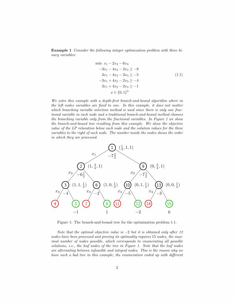
Example 1 Consider the following integer optimization problem with three bi-nary variables:

min x1 − 2x2 − 6x3

−3x1 − 4x2 − 2x3 ≥ −8

3x1 − 4x2 − 2x3 ≥ −5 (1.1)

−3x1 + 4x2 − 2x3 ≥ −4

3x1 + 4x2 − 2x3 ≥ −1

x ∈ {0, 1}3

We solve this example with a depth-first branch-and-bound algorithm where inthe left nodes variables are fixed to one. In this example, it does not matterwhich branching variable selection method is used since there is only one frac-tional variable in each node and a traditional branch-and-bound method choosesthe branching variable only from the fractional variables. In Figure 1 we showthe branch-and-bound tree resulting from this example. We show the objectivevalue of the LP relaxation below each node and the solution values for the threevariables to the right of each node. The number inside the nodes shows the orderin which they are processed.

1

−7 23

( 13 , 1, 1)

2

−6 12

(1, 34 , 1)

3

−4

(1, 1, 12 )

4

x3

5

−1

x2

6

−2

(1, 0, 12 )

7

x3

8

1

x1

9

−7 12

(0, 34 , 1)

10

−5

(0, 1, 12 )

11

x3

12

−2

x2

13

−3

(0, 0, 12 )

14

x3

15

0

Figure 1: The branch-and-bound tree for the optimization problem 1.1.

Note that the optimal objective value is −2 but it is obtained only after 12nodes have been processed and proving its optimality requires 15 nodes, the max-imal number of nodes possible, which corresponds to enumerating all possiblesolutions, i.e., the leaf nodes of the tree in Figure 1. Note that the leaf nodesare alternating between infeasible and integral nodes. This is the reason why wehave such a bad tree in this example; the enumeration ended up with different

2

types of leaf nodes next to each other. Hence the branch-and-bound method hasno chance to prune several leaf nodes together early on at a common ancestor.

Research on branch-and-bound algorithms has put a huge emphasis on mak-ing the decisions in the algorithm in such a way as to avoid enumeration of largeparts of the solution space. Especially selecting the branching variables has beenstudied extensively (see, for example, [1]), because which branching variable ischosen determines the shape of the tree of a branch-and-bound method and thushow many nodes need to be processed. In this paper we will present an imple-mentation for a branch-and-bound method that follows a different approach inwhich the shape of the tree can be changed. This means that we want to have abranch-and-bound algorithm where the decisions on the branching variables canbe deferred to a time when potentially more information is available to makethese decisions. Example 2 demonstrates that the same problem from Example1 can be solved more efficiently if the branch-and-bound tree has a differentshape.

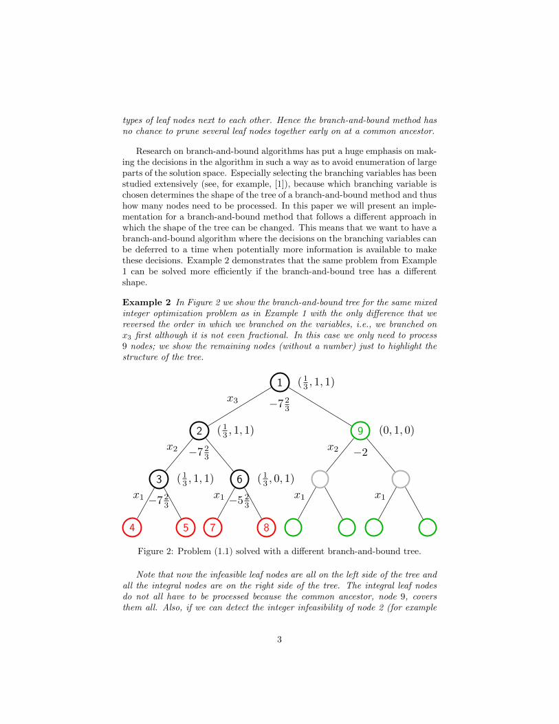
Example 2 In Figure 2 we show the branch-and-bound tree for the same mixedinteger optimization problem as in Example 1 with the only difference that wereversed the order in which we branched on the variables, i.e., we branched onx3 first although it is not even fractional. In this case we only need to process9 nodes; we show the remaining nodes (without a number) just to highlight thestructure of the tree.

1

−7 23

( 13 , 1, 1)

2

−7 23

( 13 , 1, 1)

3

−7 23

( 13 , 1, 1)

4

x1

5

x2

6

−5 23

( 13 , 0, 1)

7

x1

8

x3

9

−2

(0, 1, 0)

x1

x2

x1

Figure 2: Problem (1.1) solved with a different branch-and-bound tree.

Note that now the infeasible leaf nodes are all on the left side of the tree andall the integral nodes are on the right side of the tree. The integral leaf nodesdo not all have to be processed because the common ancestor, node 9, coversthem all. Also, if we can detect the integer infeasibility of node 2 (for example

3

with probing or some other node presolver technique), then we can prune all thenodes below it and solve the problem even faster. The lesson is that it is better tohave a tree in which nodes with similar properties are the leaf nodes of subtreesso that they can be dealt with at a common ancestor.

The question here is twofold. First, we need to reshape the tree if we believethat the current tree structure is inefficient. The second question is equallyimportant: we need to do this in an efficient way, so that we can preservemost of the advanced techniques that make branch-and-bound implementationsperform well in practice. While it is possible to simply throw away most of thetree and roll back to the last known good decision point (or variants thereofcalled restarting as, for example, discussed in [1]), we want to explicitly lookinto other possibilities here.

There has been some research in branch-and-bound methods with an ad-justable (sometimes called dynamic) tree. The earliest we are aware of is byGlover and Tangedahl [6]. Chvatal in [3] and then Hanafi and Glover in [7] re-visited the topic. These papers give valuable insights into alternative methodsfor solving mixed integer optimization problems but unfortunately do not dis-cuss the implementational challenges. Furthermore, resolution search from [3],for example, is not similar enough to a classic branch-and-bound method suchthat many of the methods modern solvers successfully use to solve problemstoday are not directly applicable.

2 Diving, Shaping, and Trimming

In this section we discuss three very important concepts for the remainder ofthis paper: diving, shaping, and trimming. We do so using a depth-first branch-and-bound method because these concepts are easier to explain in this methodand are also a natural extension to it.

Depth first branch-and-bound (sometimes also called last-in-first-out, i.e.LIFO, branch-and-bound) is a variant of branch-and-bound where the next nodeprocessed is always the most recent node added to a stack of open nodes. Inpractice it is possible to store the open nodes with a stack of bound changes.The depth-first branch-and-bound method also minimizes the number of opennodes. The result is a very memory-efficient branch-and-bound method.

In the depth-first branch-and-bound method we repeatedly go down thetree only changing one variable at a time. We call this process of going downa tree diving. Another advantage of the depth-first branch-and-bound methodis that the LP relaxations during diving can be solved very efficiently usinga dual simplex algorithm where most data structures (most importantly thefactorization of the basis matrix) can be kept up to date. We call this hotstartingthe dual simplex to express that it is even better than warmstarting, whichtypically implies that a known dual feasible basis is used to initialize the dualsimplex algorithm. When backtracking in the depth-first branch-and-boundwe cannot use hotstarting, but since the difference between nodes is typically

4

small we can warmstart from the last basis instead of resolving from scratch.Since diving is much more efficient, current implementations of non-depth-firstbranch-and-bound methods also use it to process nodes quickly and only do afull node selection if the current dive does not seem promising anymore.

The disadvantage of the depth-first branch-and-bound method is that theproblem described in the introduction is aggravated: a bad decision early on canresult in a very bad enumeration tree and thus long running time or a failure tosolve the problem within some resource limitation. But it is also much easier torevise earlier decisions and change the order of bound changes in a dive. Noticethat for the status of the final node in a dive the order in which the variableswere fixed does not matter. The order of the bound changes in a dive in somesense defines the shape of the branch-and-bound tree. Hence we call changingthe order of the bound changes in a dive shaping. Since in a depth-first branch-and-bound we store the bound changes in a stack we can decide to undo themin a different order than we did them during the dive. The only thing we haveto keep in mind is that we can only change the order of the bound changes upto the last node where we have already explored the other side of the boundchange.

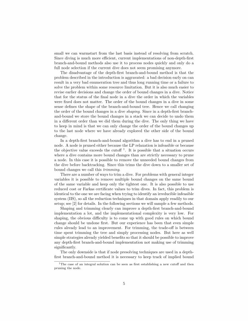
In a depth-first branch-and-bound algorithm a dive has to end in a prunednode. A node is pruned either because the LP relaxation is infeasible or becausethe objective value exceeds the cutoff 1. It is possible that a situation occurswhere a dive contains more bound changes than are strictly necessary to prunea node. In this case it is possible to remove the unneeded bound changes fromthe dive before backtracking. Since this trims the dive down to a smaller set ofbound changes we call this trimming.

There are a number of ways to trim a dive. For problems with general integervariables it is possible to remove multiple bound changes on the same boundof the same variable and keep only the tightest one. It is also possible to usereduced cost or Farkas certificate values to trim dives. In fact, this problem isidentical to the one we are facing when trying to identify an irreducible infeasiblesystem (IIS), so all the reduction techniques in that domain apply readily to oursetup; see [2] for details. In the following sections we will sample a few methods.

Shaping and trimming clearly can improve a depth-first branch-and-boundimplementation a lot, and the implementational complexity is very low. Forshaping, the obvious difficulty is to come up with good rules on which boundchange should be undone first. But our experience has been that even simplerules already lead to an improvement. For trimming, the trade-off is betweentime spent trimming the tree and simply processing nodes. But here as wellsimple strategies already yielded benefits so that it should be possible to improveany depth-first branch-and-bound implementation not making use of trimmingsignificantly.

The only downside is that if node presolving techniques are used in a depth-first branch-and-bound method it is necessary to keep track of implied bound

1The case of an integral solution can be seen as first establishing a new cutoff and thenpruning the node.

5

changes separately from the actual branching decisions. As a result, duringbacktracking some tightenings from node presolve have to be redone.

The concepts of shaping and trimming the tree already appear in principlein [6], but that paper does not include any implementational considerations.

3 A New Branch-and-bound Method

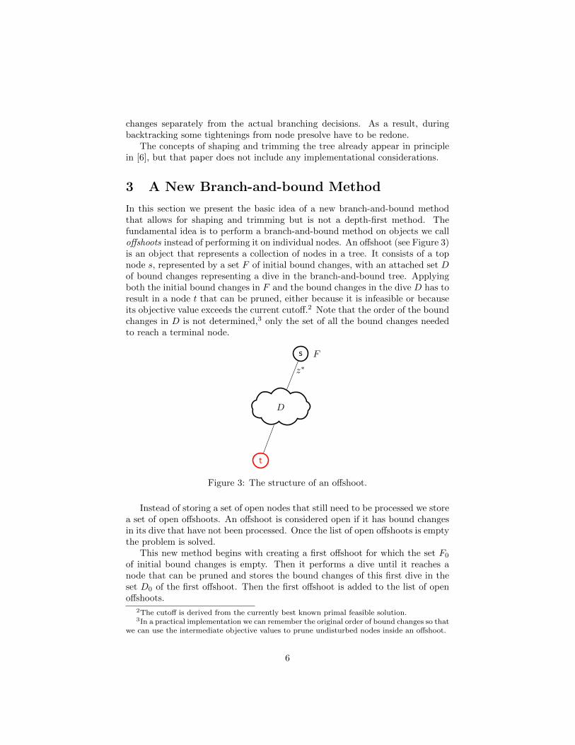
In this section we present the basic idea of a new branch-and-bound methodthat allows for shaping and trimming but is not a depth-first method. Thefundamental idea is to perform a branch-and-bound method on objects we calloffshoots instead of performing it on individual nodes. An offshoot (see Figure 3)is an object that represents a collection of nodes in a tree. It consists of a topnode s, represented by a set F of initial bound changes, with an attached set Dof bound changes representing a dive in the branch-and-bound tree. Applyingboth the initial bound changes in F and the bound changes in the dive D has toresult in a node t that can be pruned, either because it is infeasible or becauseits objective value exceeds the current cutoff.2 Note that the order of the boundchanges in D is not determined,3 only the set of all the bound changes neededto reach a terminal node.

s F

z∗

D

t

Figure 3: The structure of an offshoot.

Instead of storing a set of open nodes that still need to be processed we storea set of open offshoots. An offshoot is considered open if it has bound changesin its dive that have not been processed. Once the list of open offshoots is emptythe problem is solved.

This new method begins with creating a first offshoot for which the set F0

of initial bound changes is empty. Then it performs a dive until it reaches anode that can be pruned and stores the bound changes of this first dive in theset D0 of the first offshoot. Then the first offshoot is added to the list of openoffshoots.

2The cutoff is derived from the currently best known primal feasible solution.3In a practical implementation we can remember the original order of bound changes so that

we can use the intermediate objective values to prune undisturbed nodes inside an offshoot.

6

From now on, in each iteration, the method selects an offshoot from thelist of open offshoots as parent offshoot p for a new offshoot k to create.The method also needs to select a bound change to process associated withan offshoot variable i from the list Dp of unprocessed dive bound changesof its parent. The initial set of bound changes for the new offshoot k isFk = Fp ∪ (Dk \ {xi ≤ b}) ∪ {xi ≥ b + 1} if the bound change for the selectedvariable was branching down or Fk = Fp ∪ (Dk \ {xi ≥ b}) ∪ {xi ≤ b− 1} if itwas branching up. The new offshoot starts with a node that corresponds to aright node of the dive but since we can freely choose from all bound changes inthe dive it might be a right node that does not correspond to any of the divenodes that were processed when the offshoot was created. This choosing of thevariable from the dive corresponds to shaping the tree.

After creating the initial node of the new offshoot we solve the LP relaxationof the top node in the new offshoot. If the top node can be pruned we proceedby selecting a new parent offshoot right away. Otherwise we store the objectivevalue as the top bound z∗k of the new offshoot. Then we perform a dive untilwe reach a node that can be pruned either because it is infeasible or because itsobjective value exceeds the current cutoff. If we encounter a new primal feasiblesolution we update the cutoff. When updating the cutoff we can also remove allopen offshoots for which the top bound exceeds the cutoff.4

In this setup we can also easily perform trimming. As mentioned before,this can be done, for example, by removing multiple bound changes on thesame bound of a variable (only in the case of general integer variables) or byinspecting the dual information of the pruned node. To specify in more detail:the dual information vector r is either the reduced cost vector for cutoff nodes orthe Farkas certificate for infeasible nodes. An upper bound change on variablei can be removed if ri ≥ 0, and a lower bound change on variable i can beremoved if ri ≤ 0.

After trimming the dive we can store the new offshoot in the list of openoffshoots and remove the parent offshoot if all the bound changes in its divehave been processed.

This continues until the list of open offshoots is empty. Figure 4 shows anexample where the new method is applied to Example 1.

4 Improvements and Extensions

As with many similar methods it is necessary to improve and extend our newmethod to get the best possible performance. In this section we list some moreor less obvious ways to overcome some of the weaknesses of the new method.

4In addition, we can also remove those nodes inside offshoots that have not been disturbedyet if their objective value exceeds the cutoff.

7

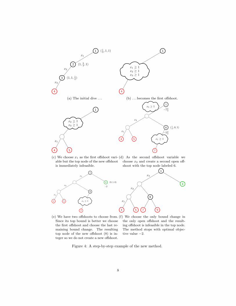
1 ( 13 , 1, 1)

2 (1, 34 , 1)

3 (1, 1, 12 )

4

x3

x2

x1

(a) The initial dive . . .

1

4

x1 ≥ 1x2 ≥ 1x3 ≥ 1

(b) . . . becomes the first offshoot.

1

x2 ≥ 1x3 ≥ 1

4

x1

5

(c) We choose x1 as the first offshoot vari-able but the top node of the new offshootis immediately infeasible.

1

−7 23

4

x1

5

x2

6

−5 23

( 13 , 0, 1)

x1 ≥ 1

7

x3 ≥ 1

(d) As the second offshoot variable wechoose x2 and create a second open off-shoot with the top node labeled 6.

1

4

x1

5

x2

6

x1 ≥ 1

7

x3

8

−2

(0, 1, 0)

(e) We have two offshoots to choose from.Since its top bound is better we choosethe first offshoot and choose the last re-maining bound change. The resultingtop node of the new offshoot (8) is in-teger so we do not create a new offshoot.

1

4

x1

5

x2

6

7 9

x3

8

(f) We choose the only bound change inthe only open offshoot and the result-ing offshoot is infeasible in the top node.The method stops with optimal objec-tive value −2.

Figure 4: A step-by-step example of the new method.

8

p Fp

z∗

D \ {xi ≥ 1}

t k Fk

xi ≤ 0

(a) Branching from the bottom

p

z∗

Fp∪{xi ≥ 1}

D \ {xi ≥ 1}

t

k Fk

xi ≤ 0

(b) Branching from the top

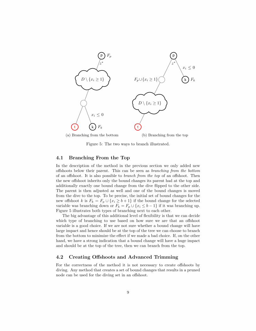
Figure 5: The two ways to branch illustrated.

4.1 Branching From the Top

In the description of the method in the previous section we only added newoffshoots below their parent. This can be seen as branching from the bottomof an offshoot. It is also possible to branch from the top of an offshoot. Thenthe new offshoot inherits only the bound changes its parent had at the top andadditionally exactly one bound change from the dive flipped to the other side.The parent is then adjusted as well and one of the bound changes is movedfrom the dive to the top. To be precise, the initial set of bound changes for thenew offshoot k is Fk = Fp ∪ {xi ≥ b + 1} if the bound change for the selectedvariable was branching down or Fk = Fp ∪ {xi ≤ b− 1} if it was branching up.Figure 5 illustrates both types of branching next to each other.

The big advantage of this additional level of flexibility is that we can decidewhich type of branching to use based on how sure we are that an offshootvariable is a good choice. If we are not sure whether a bound change will havelarge impact and hence should be at the top of the tree we can choose to branchfrom the bottom to minimize the effect if we made a bad choice. If, on the otherhand, we have a strong indication that a bound change will have a huge impactand should be at the top of the tree, then we can branch from the top.

4.2 Creating Offshoots and Advanced Trimming

For the correctness of the method it is not necessary to create offshoots bydiving. Any method that creates a set of bound changes that results in a prunednode can be used for the diving set in an offshoot.

9

One slight modification to the method is to apply several bound changes atonce before solving an LP relaxation. We call this plunging. This can go as faras fixing all integer variables since the result is guaranteed to be pruned andtrimming can then be used to reduce the set of bound changes.

Another possibility is to use conflict analysis as described in [1] to obtain aclause. For offshoots that end in an infeasible node the dive set of bound changesis precisely a clause. Hence it is also possible to apply the method described byKarzan et al. in [8] to obtain a minimal clause using a MIPing approach.

4.3 Improved Pruning

One of the disadvantages of the new method is that pruning by bound after anew primal feasible solution has been found is complicated. Obviously, we canprune whole offshoots as soon as their top bound exceeds the new bound. But itcan happen that for some offshoots the top bound is not large enough althoughapplying some of the bound changes from the dive would result in an LP boundthat would lead to a pruning.

This issue can be overcome partially by storing the objective values obtainedduring a dive. As long as no new offshoot is created from the dive (or newoffshoots are created only from the bottom and in the order of the original dive)we can use the objective values to trim the dives after a new bound has beenfound. Since trimming also invalidates the bounds from the dive it is advisableto delay trimming until we first want to create an offshoot. This requires slightlymore memory since more bound changes and dual information might have tobe stored, but it could result in significantly better performance.

4.4 Bounding Offshoots

When branching from the top, the top bound of an offshoot remains a validbound on all the nodes below this offshoot. But since we add a bound changeto the top of the offshoot the bound is obviously not as strong as it could be.Hence it might be worthwhile updating the top bound after branching from thetop.

We propose three methods of increasing computational effort to strengthenthe bound. The first method is to derive a bound on the top node of theparent offshoot by using the reduced cost of the just-solved top node of the newoffshoot.

The second method is a bit more general but also requires more computa-tional effort. It involves simply evaluating the dual solution of the new offshoot’stop node for the bounds of the parent offshoot.

The third method is to solve the LP for the new top node of the parentoffshoot. Since we have a warmstart basis from the top node of the new offshootthis can be done using a very good warmstart basis.

Obviously, the first two methods provide only a lower bound on the newoptimal objective value.

10

4.5 Shortening Dives

It is possible to implement the new method in a way that traditional branch-and-bound is just a special case. To this end we only need to ensure that inaddition to storing open offshoots we can also store open nodes. This can beachieved, for example, by treating offshoots without a dive as normal nodes,which means when we select them we do not select an offshoot variable. Insteadwe treat it as the top node of a new offshoot directly. With this in place we canalso have a limit on the number of bound changes in a dive. When the limit ishit, we store the last node as an open node in addition to storing the offshoot.The offshoot in this case does not end in a pruned node, but the method worksregardless. If we set the limit of bound changes in a dive to zero, the methodreverts to a traditional branch-and-bound method.

4.6 Splitting offshoots

Branching from the top on a bound change that was not the initial boundchange of an offshoot invalidates all the internal objective values of the origi-nal nodes of an offshoot. This prevents us from pruning them and hurts theperformance for very deep dives. Therefore it seems advantageous to split verylong dives. However, this creates a non-terminal offshoot, so it extends ourdepth-first framework a little. For maximum efficiency, we need to resolve thelinear relaxation of the bottom offshoot, so that we can have a valid objectivevalue useful for pruning by bound. Which bound changes should be in the topof bottom half of the split is an interesting research question.

5 Computational Evaluation

The new method was prototyped using the MILP solver in SAS/OR. The pro-totype was meant as a way to evaluate the correctness and practicability of themethod described and as such does not contain all the features and tricks of afull MILP solver. Nevertheless we present results using this prototype to givean impression of the capabilities of the new method.

The prototype plugs into the MILP solver after its root node when the actualbranch-and-bound phase begins. It features a standard reliability branchingstrategy with a dynamic strong branching limit and a reliability limit of 5. Forselecting the next offshoot we choose the best top bound first without explicittie breaking. The prototype also features basic node presolve and reduced costfixing techniques (only at the top of an offshoot), and also using the root reducedcost to fix columns globally as new incumbent solutions are found. What itnotably lacks are more advanced node presolver techniques, local or global cutsin the nodes of the branch-and-bound tree, and primal heuristics.

We conduct our experiments on 96 machines running 2 jobs each on 16-core/2-socket IntelR© XeonR© E5-2630 v3 @ 2.40GHz CPUs. All experimentsare done with default settings, a memory limit of 62 GB, and a time limit of2 hours. We use 798 instances that are the internal test set used to develop

11

the SAS MILP solver. To evaluate our results we use performance profiles asdescribed in [5].

5.1 Offshoot variable selection

The first experiment evaluates several methods we implemented for choosingthe offshoot variable, i.e., it is meant to judge the importance of shaping in thenew method. We implemented four different methods:

bottom: always branch from the bottom of an offshoot without changing theorder of the variables;

top: always branch from the top of an offshoot without changing the order ofthe variables;

pseudo: choose the offshoot variable with the best reliable pseudocost scoreand branch from the top. If there are no offshoot variables with reliablepseudocost available, then choose the variable with the worst pseudocostscore and branch from the bottom.

pseudodual: like pseudo, except if there are no variables with reliable pseu-docost then use the variable with the worst dual information score andbranch from the bottom. The dual information score is the reduced costor the Farkas certificate of the pruned node when the offshoot was firstprocessed.

The first two strategies do not shape the tree so they can be seen as a baselinefor the performance of the method. The default method is pseudodual.

Figure 6 shows the performance profile comparing the different offshoot vari-able selection strategies. In addition we would like to mention that the pseudo-dual strategy is about 13% faster in the geometric mean of the solve times thanthe bottom strategy and solves 9 instances more within the time limit. Weargue that this shows that shaping, at least in the context of this new method,has a clear impact on the performance. More advanced selection strategies canprobably be developed that will demonstrate this even more profoundly.

5.2 Trimming and pruning

Our second experiment is designed to show the combined importance of trim-ming and pruning. In our prototype implementation we delay trimming anoffshoot until we need to choose an offshoot variable for the first time. Since wecan either prune the bottom of the offshoot using the current cutoff or applytrimming using the dual information, we analyze how many reductions we getfrom either and choose the method that yields the most. In this experimentwe compare the default version of our prototype that does this delayed pruningor trimming with a version where this feature has been disabled. The perfor-mance profile can be seen in Figure 7. The version with trimming and pruningis about 5% faster in the geometric mean of solve times and solves 1 instance

12

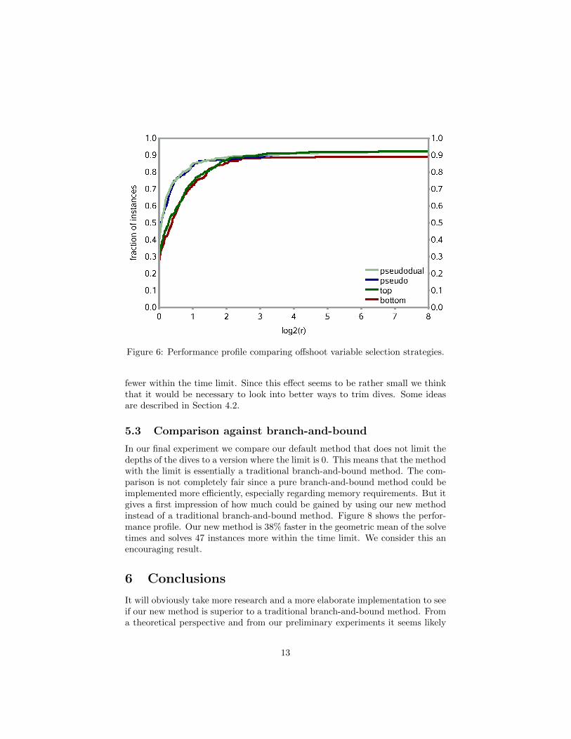
Figure 6: Performance profile comparing offshoot variable selection strategies.

fewer within the time limit. Since this effect seems to be rather small we thinkthat it would be necessary to look into better ways to trim dives. Some ideasare described in Section 4.2.

5.3 Comparison against branch-and-bound

In our final experiment we compare our default method that does not limit thedepths of the dives to a version where the limit is 0. This means that the methodwith the limit is essentially a traditional branch-and-bound method. The com-parison is not completely fair since a pure branch-and-bound method could beimplemented more efficiently, especially regarding memory requirements. But itgives a first impression of how much could be gained by using our new methodinstead of a traditional branch-and-bound method. Figure 8 shows the perfor-mance profile. Our new method is 38% faster in the geometric mean of the solvetimes and solves 47 instances more within the time limit. We consider this anencouraging result.

6 Conclusions

It will obviously take more research and a more elaborate implementation to seeif our new method is superior to a traditional branch-and-bound method. Froma theoretical perspective and from our preliminary experiments it seems likely

13

Figure 7: Performance profile comparing a version of the prototype that doespruning and trimming with a version that does not.

that shaping and trimming the tree will result in improved run times. Even ifthe performance gains end up being very small there is also hope that our newmethod will result in a more stable performance.

So far we have not investigated other areas of application for our new methodsuch as mixed integer non-linear optimization problems or branch-and-pricealgorithms. Since in these areas more flexibility in the tree might be even moreadvantageous we hope that it will find application there as well.

References

[1] T. Achterberg, T. Koch, and A. Martin, Branching rules revisited, Opera-tions Research Letters 33 (2005), no. 1, 42–54.

[2] J. W. Chinneck, Feasibility and infeasibility in optimization: Algorithmsand computational methods, International Series in Operations Research andManagement Sciences, vol. 118, 2008.

[3] V. Chvatal, Resolution search, Discrete Applied Mathematics 73 (1997),no. 1, 81 – 99.

[4] W. Cook, Markowitz and Manne+ Eastman+ Land and Doig= branch andbound, Optimization Stories (2012), 227–238.

14

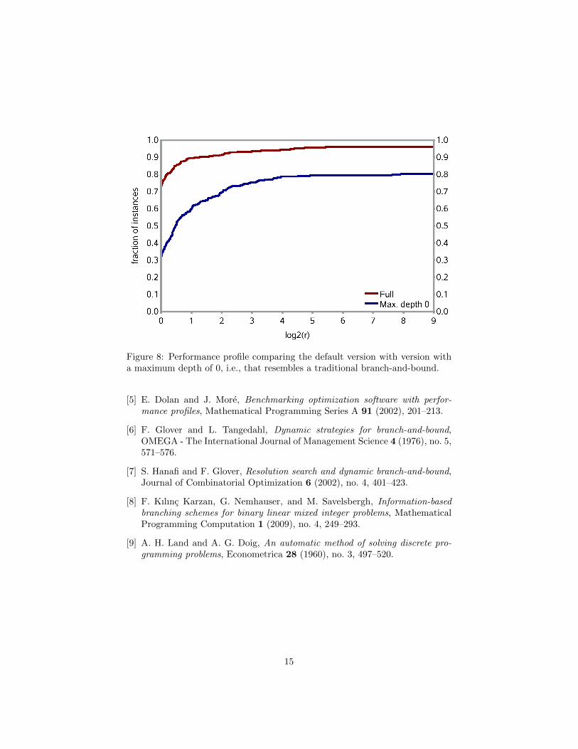
Figure 8: Performance profile comparing the default version with version witha maximum depth of 0, i.e., that resembles a traditional branch-and-bound.

[5] E. Dolan and J. More, Benchmarking optimization software with perfor-mance profiles, Mathematical Programming Series A 91 (2002), 201–213.

[6] F. Glover and L. Tangedahl, Dynamic strategies for branch-and-bound,OMEGA - The International Journal of Management Science 4 (1976), no. 5,571–576.

[7] S. Hanafi and F. Glover, Resolution search and dynamic branch-and-bound,Journal of Combinatorial Optimization 6 (2002), no. 4, 401–423.

[8] F. Kılınc Karzan, G. Nemhauser, and M. Savelsbergh, Information-basedbranching schemes for binary linear mixed integer problems, MathematicalProgramming Computation 1 (2009), no. 4, 249–293.

[9] A. H. Land and A. G. Doig, An automatic method of solving discrete pro-gramming problems, Econometrica 28 (1960), no. 3, 497–520.

15