shape recognition for plane closed …jmconrad/gradstudents/thesis...dr. conrad has been an idol to...
TRANSCRIPT

SHAPE RECOGNITION FOR PLANE CLOSED CURVES USING ERRORMODEL OF AN ELLIPTICAL FIT AND FOURIER DESCRIPTORS
by
Onkar Nitin Raut
A dissertation submitted to the faculty ofThe University of North Carolina at Charlotte
in partial fulfillment of the requirementsfor the degree of Master of Science in
Electrical Engineering
Charlotte
2011
Approved by:
Dr. James M. Conrad
Dr. Ronald R. Sass
Dr. Thomas P. Weldon

ii
c© 2011
Onkar Nitin Raut
ALL RIGHTS RESERVED

iii
ABSTRACT
ONKAR NITIN RAUT. Shape recognition for plane closed curves using error modelof an elliptical fit and Fourier descriptors. (Under the direction of DR. JAMES M.
CONRAD)
Since the past few decades there has been profound interest shown in robotics
and computer vision specially towards object recognition. While there are many
techniques available to choose from, an investigation is carried out in this work on
techniques that use Fourier descriptors for analyzing and modelling objects of inter-
est. Also, a new technique for generating Fourier descriptors is designed and the
performance is evaluated against existing techniques for generating Fourier descrip-
tors. This new technique generates the Fourier descriptor by fitting an ellipse to a
shape normalized boundary segment extracted from an image of a plane close object
and finding the error of the fit. This error forms the signal input for generating the
Fourier descriptor.
Experiments are performed using the new technique which involve classifying a
database of leaves using a simple k-Nearest Neighbours classifier. Results deduced
from the performance of this newly designed technique indicate improved consistancy
and accuracy over previous methods. This encouraged the development of a real
time recognition system used to recognize known objects of interest in an unknown
environment as an application towards computer vision and robotics.

iv
ACKNOWLEDGMENTS
The work presented in this document would not have been possible without the
support of my advisor Dr. James M. Conrad and his confidence in my proposed work.
Dr. Conrad has been an idol to me when it comes to both education and profession-
alism. I have constantly enjoyed working with him and for him on numerous research
occasions. He has been a constant source of motivation and guidance throughout
the course of my Master’s program in Electrical Engineering. I express my sincere
gratitude towards Dr. Conrad for helping me believe in my capabilities. I am also
grateful to my committee members Dr. Thomas Weldon and Dr. Ronald Sass for
their advice, time and support provided for this work.
I would like to thank my parents, Smita and Nitin Raut for encouraging my further
studies without any forms of parental pressure. Their support and faith in my success
has provided me with the motivation to constantly better myself in every aspect of
my life.
Finally, I would like to thank my colleague Suraj Swami for being a constant
challenge towards my approach in solving problems posed in this work and numerous
projects we worked on together. I would like to thank my friends Jerry Zacharias,
Thomas Meiswinkel, Malcolm Zapata and many others for inspiring me to take up
multiple challenges throughout the Master’s program, all of which has culminated
towards this thesis.

v
TABLE OF CONTENTS
LIST OF FIGURES vii
LIST OF TABLES ix
LIST OF ABBREVIATIONS x
CHAPTER 1: INTRODUCTION 1
1.1 Motivation 1
1.2 Problem Statement 3
1.3 Contribution 3
1.4 Organization of the thesis 4
CHAPTER 2: BACKGROUND 5
2.1 Discrete Fourier Transform 5
2.2 Morphological Image Processing 6
2.2.1 Basics of set theory 7
2.2.2 Image Dilation 8
2.2.3 Image Erosion 9
2.2.4 Boundary Extraction 9
2.2.5 Connected Components 9
2.3 Polynomial Fitting 10
2.4 Polynomial Fitting to two dimensional data (Fitting Ellipses) 13
2.5 Problem Statement of Recognition 15
2.6 Problem Statement of Shape Analysis 17
CHAPTER 3: TECHNIQUES FOR SHAPE ANALYSIS 18
3.1 Models For Shape Analysis and Representation 18

vi
3.1.1 Chain Codes 18
3.1.2 Polygon Approximation 19
3.1.3 Signatures 20
3.1.4 Skeletons (Medial Axis Transformation) 21
3.1.5 Shape Numbers 21
3.1.6 Statistical Moments 21
3.1.7 Fourier Descriptors 23
3.2 Properties of Fourier Descriptors 23
3.3 Techniques for generating Fourier Descriptors 25
3.4 Previous work on Fourier Descriptors 27
CHAPTER 4: DESIGN AND TESTING 32
4.1 Algorithm 33
4.2 Testing 38
4.3 Hardware Design 45
4.4 Software Design 47
CHAPTER 5: EVALUATION 51
CHAPTER 6: CONCLUSION 58
BIBLIOGRAPHY 60
APPENDIX A: SOURCE CODE 62
A.1 Project Structures 62
A.2 Program codes 64
vii
LIST OF FIGURES
FIGURE 1.1: Quadrotor design for Charlotte Area Robotics 2
FIGURE 2.1: Sample signal, magnitude and phase plots 6
FIGURE 3.1: 4-connected and 8-connected chain codes 19
FIGURE 3.2: An example signature of a circle 20
FIGURE 3.3: Shape Number of order 18 22
FIGURE 3.4: Rotating a boundary to create a histogram 23
FIGURE 4.1: Flowchart (part 01) 36
FIGURE 4.2: Flowchart (part 01) 37
FIGURE 4.3: Samples from image database used 39
FIGURE 4.4: Database used by Zhang, D. and Lu, G. 41
FIGURE 4.5: Results of segmentation and boundary extraction 41
FIGURE 4.6: Examples of incorrect segmentation 41
FIGURE 4.7: Fitting an ellipse to extracted boundary data 43
FIGURE 4.8: Boundary with no shape normalization 43
FIGURE 4.9: Boundary with shape normalization 44
FIGURE 4.10: Addition of noise to boundary data 45
FIGURE 5.1: Sample training images, class 01 55
FIGURE 5.2: Sample training images, class 02 55
FIGURE 5.3: Sample training images, class 03 56
FIGURE 5.4: Realtime recognition of class 01 56
FIGURE 5.5: Realtime recognition of class 02 56
FIGURE 5.6: Realtime recognition of class 03 56

viii
FIGURE 5.7: Realtime recognition failure 57
FIGURE A.1: Training Module Project Structure. 62
FIGURE A.2: Classification Module Project Structure. 63

ix
LIST OF TABLES
TABLE 5.1: Comparison of classification results, class 01 52
TABLE 5.2: Comparison of classification results, class 02 52
TABLE 5.3: Comparison of classification results, class 03 52
TABLE 5.4: Average time for computation(Test system) 53
TABLE 5.5: Comparison of classification results with added noise, class 01 54
TABLE 5.6: Comparison of classification results with added noise, class 02 54
TABLE 5.7: Comparison of classification results with added noise, class 03 55

LIST OF ABBREVIATIONS
AI Artificial Intelligence
BBxM BeagleBoard-xM
CAR Charlotte Area Robotics
DFT Discrete Fourier Transform
FD Fourier Descriptor
kNN k-Nearest Neighbour
OpenCV Open-source Computer Vision
USB Universal Serial Bus

CHAPTER 1: INTRODUCTION
1.1 Motivation
In Fall 2010, Charlotte Area Robotics (CAR), a student organization at the Uni-
versity of North Carolina at Charlotte, proposed a task of developing an autonomous
quadrotor capable of navigating indoor environments. One of the major challenges
issued included detection of objects of interest using an overhead camera mounted
at the base of the hovering quadrotor. The overall objective of the project was to
navigate the indoor environment successfully and retrieve the object of interest.
While it is almost effortless for humans to recognize an object, it is a tedious
task to make machines understand them. Object detection and recognition is a field
under Machine Learning and Computer Vision that is being explored since the past
few decades. An initial study of available techniques for object recognition proved
to be quite overwhelming. Some of the widely known techniques one might come
across while investigating the topic include the use of Affine Invariant Transforms
for Feature Detection and Recognition, Hough Transform, Ridge Detection, Scale-
invariant feature transform, Speeded Up Robust Features, Gradient Location and
Orientation Histogram, Histogram of Oriented Gradients and Local Energy-based
Shape Histogram.
One key aspect of the environment in which the object of interest is located is
that it is non-cluttered, i.e. there is no overlap of other objects on the one of inter-

2
Figure 1.1: Quadrotor design for Charlotte Area Robotics
est. If this aspect of the environment is exploited correctly, it can prove beneficial
towards providing good features, thereby allowing better classification. Being in a
non-cluttered environment, object recognition can be performed by either discrim-
inating the shapes or textures of different objects. Since a planar camera is used,
“shape” in this case is dictated by the outline i.e boundary of the object.
Due to the non-deterministic nature of the location of the object, the technique
chosen to perform recognition needs to be independent of translation, rotation and
scale of the object of interest. Independence from translation allows recognition to
succeed independent of the position of the object. Independence from rotation ensures
that recognition succeeds when the object is not in the same pose during training,
where as independence from scaling allows recognition to succeed when the object
is not the same size as during training. This allows the system to conform to the
stochastic nature of the real world. These parameters greatly reduce the amount
of training and testing required for a classifier, thereby reducing the computational
cost and time. While being invariant to translation rotation and scaling, the method
must also be robust, that is, invariant to noise to a certain extent. Recognition using

3
Fourier Descriptors (FDs) is one such technique that fulfills the above criteria.
Recognition in this case is performed on the most recent acquired image of an
object by extracting features of the object from the image and performing statistical
analysis against a known database of features of the object of interest. The end
goal of this work is to investigate recognition of non-occluded objects in images using
FDs using the error model of an elliptical fit to the data. This is the new technique
created and analysed in this work. Since there are other techniques for generating
FDs, a common database for classification is selected to determine the accuracy of
classification with the newly designed technique against the old techniques.
1.2 Problem Statement
The problem statement of this work is formulated into four parts:
1. Create a new model for acquiring FDs.
2. Investigate the accuracy of recognition using FDs generated using the error
model of an elliptical fit to the given data against old techniques i.e. FDs
generated using the data as complex co-ordinates and centroid distance.
3. Develop a real time testing system to perform recognition of objects using the
designed algorithm.
4. Evaluate the performance of the real time system.
1.3 Contribution
This work evaluates the performance of FDs towards the task of recognition using
a newly designed technique in this work which is based on the error model of an
elliptical fit to boundary data of plane closed curves (objects). Most of this work will

4
be incorporated into the CAR quadrotor robot for recognizing the object of interest
in the non-cluttered environment. While translating the algorithm from MATLAB R©
code to C++, it was found that there was no equivalent code for the function “polyfit”
found in MATLAB. A C++ version of the polyfit function was therefore written
using the Open-source Computer Vision (OpenCV) library and submitted to the
OpenSource community which is now included in in further releases of the OpenCV
[16].
1.4 Organization of the thesis
Chapter 1 provides an introduction to the rest of the report and the problem
statement at hand. Chapter 2 prepares the reader with the necessary mathematical
background for material introduced in Chapter 3 and 4. Chapter 3 mentions some
of the existing techniques for shape analysis, previous work and applications of FDs.
Chapter 4 details the design aspect of the system which includes the algorithm for
generating features using the error model of an elliptical fit to data, the necessary
hardware and software required to develop the test system and the real time system.
In Chapter 5, the design of the system is evaluated by discussing the results obtained.

CHAPTER 2: BACKGROUND
This chapter describes some of the earlier work on shape recognition using FDs.
It also introduces the mathematical concepts required to understand the process of
shape recognition using the design mentioned in Chapter 4.
2.1 Discrete Fourier Transform
The Fourier Transform, in continous time, is a mathematical operation that de-
composes a given signal into its constituent frequencies (in Hz). However, since all
computational machines operate on a discrete clock signal, of more importance to us
is the Discrete Fourier Transform (DFT). The DFT operates on a input function or
signal that is discrete, finite and has non zero values (real or complex numbers). A
person’s sampled voice using a analog to digital converter is a good example of a input
function or signal. It only evaluates enough frequency components to reconstruct the
finite segment that was analyzed i.e. frequency mapping/evaluation is for frequencies
between 0 to 2π or −π to +π. The mathematical definition of the DFT is if a signal
x(t) is sampled at equal time intervals Ts and the corresponding analog values are
converted into their discrete representation, a signal x(n) is obtained. Assuming that
this signal x(n) is finite i.e. n = 0, 1, 2, .... N - 1, the DFT X(k) is computed as,
X(k) =N−1∑n=0
x(n)e−2πiN
kn (2.1)
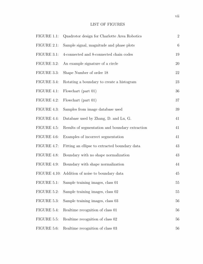
An example plot of a discrete signal along with the magnitude and phase plots
6
after applying DFT using Equation 2.1 to the signal are shown in Figure 2.1
Figure 2.1: Plot of a signal in time and the corresponding magnitude and phase plots
after applying DFT
2.2 Morphological Image Processing
The result of sampling and quantization of a scene in the real world by means of
a image capture device, such as a camera, is a matrix of real numbers, i.e. a digital
image. From here on, we will refer to the digital image as “image” only. This sampled
image f(x, y) has M rows and N columns. If f(x, y) can have either of two values,

7
0 or 1, for any given value of x and y then the image is called a binary image. If
f(x, y) can have a finite value, e.g. between 0 to 255 or say 0 to L, then the image can
be classified as a grayscale image. In general, f(x, y) is a digital image if (x, y) are
integers from Z2,the set of all ordered pairs of elements(zi, zj), with zi and zj being
integers from Z, the set of all integers and f is a function that assigns a gray level
value (that is, a real number from the set of real numbers, R) to each distinct pair of
co-ordinates (x, y).
Morphological image processing involves performing mathematical operations on
digital images based on set theory to extract image components useful for representa-
tion and description of region shape i.e., boundaries, skeleton and convex hull. Images
taken into consideration can be either binary images or images in grayscale. In or-
der to understand some of the operations introduced later, we need to understand
a few preliminary morphological operations such as image dilation and connected
components that grow into the idea of boundary extraction. These are explained in
detail in the following subsections. The following sections also introduce some of the
mathematical language that may be used in common parts of the literature.
2.2.1 Basics of set theory
Sets in mathematical morphology can represent an object in an image. For exam-
ple, all black pixels in an image form a set that can provide a complete morphological
description of the image. Let A be a set in Z2. If a = (a1, a2) is an element of A, we
write a ∈ A. If not, we write a /∈ A. If a set has no elements, we call it an empty or
null set denoted by ∅. If every element in set A is also an element in set B we write,
A ⊆ B. Union and intersection of two sets are written as C = A∪B and D = A∩B

8
respectively. Sets A and B are said to be mutually exclusive if they have no common
elements. We write this as A ∩ B = ∅. Elements not contained in set A can be said
to form another set, which is called the complementary set Ac = {w|w /∈ A}, where
w is an element in set A. The difference of two sets A and B is
A−B = {w|w ∈ A,w /∈ B} = A ∩Bc. (2.2)
The reflection of set B, written as B is defined as
B = {w|w = −b, b ∈ B}. (2.3)
Translation of a set by point z = (z1, z2), written as (A)z is defined as
(A)z = {c|c = a+ z, for a ∈ A}. (2.4)
2.2.2 Image Dilation
Two basic operators in the area of mathematical morphology are dilation and
erosion. The basic effect of a dilation operator is to gradually enlarge the boundaries
of regions in the foreground. The areas of foreground pixels grow in size while the
holes within the region tend to become smaller. If sets A and B are in Z2, then the
dilation of A by B, denoted by, A⊕B, is defined as,
A⊕B = {z| ˆ(B)z ∩ A 6= ∅} (2.5)
Set B is usually referred to as the structuring element in dilation.

9
2.2.3 Image Erosion
The basic effect of the erosion operator on a binary image is to erode away the
boundaries of regions of foreground pixels (i.e. white pixels, typically). Thus, areas
of foreground pixels shrink in size, and holes within those areas become larger. If sets
A and B are in Z2, then the erosion of A by B, denoted by,
AB = {z|(B)z ⊆ A} (2.6)
2.2.4 Boundary Extraction
In topology and mathematics in general, the boundary of a subset S of a topolog-
ical space X is the set of points which can be approached both from S and from the
outside of S. Boundary extraction is the process of obtaining all the boundary points
of a given set A. This process from a mathematical point of view can be written as,
β(A) = A− (AB) (2.7)
where B is a structuring element. In short the boundary can be obtained by first
eroding the set A by B and then performing set difference between A and its erosion
as defined in Equation 2.6.
2.2.5 Connected Components
An object in an image is represented by either pixels of similar color or by pixels
having tight connectivity. In order to show that a group of pixels represents an object
in an image, we need to establish if a group of pixels (or a pair of pixels) are connected

10
or not. To do so it must be determined if they are neighbours and their gray levels
meet a certain criterion. If V is the set of gray level values used to define adjacency,
then for a binary image, V = {1} if we are referring to adjacency of pixels with value
1. In a grayscale image, V would have more than one value. There are three types
of adjacency, 4− adjacency, 8− adjacency and m− adjacency.
• In 4 − adjacency, two pixels p and q with values from V are 4-adjacent if q is
in the set N4(p), where N4(p) is the set of horizontal and vertical neighbouring
pixels {(x + 1, y), (x − 1, y), (x, y + 1), (x, y − 1)} of a pixel p at co-ordinates
(x, y).
• In 8 − adjacency, two pixels p and q with values from V are 8-adjacent if q
is in the set N8(p), where N8(p) is the set of horizontal, vertical and diagonal
neighbouring pixels {(x+1, y+1), (x−1, y+1), (x+1, y−1), (x−1, y−1), (x+
1, y), (x− 1, y), (x, y + 1), (x, y − 1)} of a pixel p at co-ordinates (x, y).
• m− adjacency occurs when we have two pixels p and q with values from V and
either
– q is in N4(p), or
– q is in ND(p), where ND(p) is the set of diagonal pixels {(x+1, y+1), (x−
1, y + 1), (x + 1, y − 1), (x − 1, y − 1)} and the set N4(p) ∩ N4(q) has no
pixels whose value is from V .
2.3 Polynomial Fitting
Polynomial fitting, also known as curve fitting is a technique for approximating
a mathematical model (polynomial equation) to an observed set of data points. The

11
polynomial function in this case is represented as,
y(x,w) = w0 + w1x+ w2x2 + · · ·+ wMx
M =M∑j=0
wjxj; (2.8)
This can be written in matrix format as,
y = wTx where x =
1
x
x2
x3
...
xM
and w =
w0
w1
w2
w3
...
wM
(2.9)
While there are many methods to fit a polynomial model to given data one of par-
ticular interest is fitting using least squares. Assume that t is the vector representing
the actual data point values to be fit to a series x. Since the goal is to construct
a model that approximates the data t to the series x using a model based on the
coeffiecients w, an error between the actual data point and the data point generated
from the approximation will always be present. This overall error dependent on the
model w is given by,
E(w) =N∑
n=0
y(xn, w)− tn (2.10)

12
or in matrix format
E(w) =N∑
n=0
wTxn − tn = Xw − t where X =
xT0
xT1
xT2
...
xTN
N×(M+1)
and t =
t0
t1
t2
...
tN
N×1(2.11)
with x and w defined in Equation 2.9. The objective of least squares error fitting is to
minimize square of this error over available n data points of x and t. i.e. find values
of w which minimize the square of the error. The square of the error is given by,
E(w)2 = (Xw − t)T (Xw − t) = (wTXT − tT )(Xw − t) (2.12)
E(w)2 = wTXTXw − wTXT t− tTXw + tT t = wTXTXw − 2wTXT t+ ||t2|| (2.13)
Differentiating Equation 2.13 w.r.t. w and equating to zero we get,
∂E(w)2
∂w=∂{wTXTXw − 2wTXT t+ ||t2||}
∂w= 0 (2.14)
=⇒ 0 = 2XTXw − 2XT t+ 0 (2.15)
=⇒ w = (XTX)−1XT t (2.16)

13
2.4 Polynomial Fitting to two dimensional data (Fitting Ellipses)
The general algebraic representation of a conic section is given by a quadratic
equation
Ax2 +Bxy + Cy2 +Dx+ Ey + F = 0 and A, B, C are not all zeros (2.17)
discrimination amongst the four different types of conic sections is performed by
solving the discriminant
B2 − 4AC (2.18)
If B2 − 4AC > 0 then the equation represents a hyperbola. If B2 − 4AC < 0 then
the equation represents an ellipse. If B2 − 4AC = 0 then the equation represents a
parabola. If B2 − 4AC > 0 with A = C and B = 0 then the equation represents a
circle.
Equation 2.17 can be rewritten in vector form as,
xTi a = 0 where xi =
x2
xy
y2
x
y
1
and a =
A
B
C
D
E
F
(2.19)
For Equation 2.17 to represent an ellipse we need to constrain discriminant B2 −

14
4AC > 0. This constraint can be written in matrix form as,
aT
0 0 −2 0 0 0
0 1 0 0 0 0
−2 0 0 0 0 0
0 0 0 0 0 0
0 0 0 0 0 0
0 0 0 0 0 0
a = −1 where a is described as in 2.19 (2.20)
If we treat the problem of fitting an ellipse to the data points as a least squares
problem then we need to minimize the algebraic distance such that the overall error
of fitting the data points is minimized.
mina
N∑i=1
|xTi a|2 (2.21)
which can be rewritten as
mina
N∑i=1
||aTXTXa||2 (2.22)
and solved using Lagrange multipliers. The algorithm for fitting an ellipse to data
points p1, to pN where pi = xi, yi, and i = 1...N is detailed as follows.
1. Build a design matrix X
X =
x21 x1y1 y21 x1 y1 1
x22 x2y2 y22 x2 y2 1
......
......
......
x2N xNyN y2N xN yN 1
(2.23)

15
2. Build a scatter matrix, S = XT X
3. Build a constraint matrix C where,
C =
0 0 −2 0 0 0
0 1 0 0 0 0
−2 0 0 0 0 0
0 0 0 0 0 0
0 0 0 0 0 0
0 0 0 0 0 0
(2.24)
4. Find the eigenvalues of the generalized eigenvalues problem Sa = λCa and use
λn the only negative eigenvalue to compute the eigenvector which gives the best
fit parameter vector.
2.5 Problem Statement of Recognition
The word recognition literally means the identification of something as having
been previously seen, heard, known, etc. The task of recognition today has bro-
ken down into many smaller categories like aircraft recognition, automatic number
plate recognition, facial recognition, gesture recognition, handwriting recognition, iris
recognition, language recognition, magnetic ink character recognition, named entity
recognition, optical character recognition, optical mark recognition, pattern recogni-
tion, recognition of human individuals, speech recognition, etc. The most generic one
amongst these is pattern recognition where the given input value is assigned a output

16
value or a label according to a specific algorithm. Pattern recognition can be gen-
eralized depending upon the type of learning procedure used to generate the output
labels. It can be supervised learning, wherein a set of training data is provided with
instances that have been assigned a correct label by hand or unsupervised learning,
which on the other hand, assumes training data that has not been hand-labeled, and
attempts to find inherent patterns in the data that can then be used to determine
the correct output value for new data instances.
In case of supervised learning, the objective is to produce a function h : X → Y
that can closely approximate the correct unkown mapping function g : X → Y (the
ground truth) which maps the input instances x ∈ X to output labels y ∈ Y , given
the training data D = {(x1, y1), (x2, y2), (x3, y3), ..., (xn, yn)}. X is the set of input
data or feature vectors, provided to the function and Y set of possible outputs, usu-
ally a set of labels. Practically, neither the distribution of X nor the ground truth
function g are known. However, they can be computed to a close approximation by
empirically collecting a large number of samples of X and hand labelling them using
the correct value of Y . Classification or recognition can be performed using proba-
blistic modelling/recognizer i.e. Bayes recognizer which is the most ideal theoritical
classifier possible, provided you know all other random distributions or one may use
other classification techniques such as Multivariate Gaussian Probability Distribu-
tion functions, k-Nearest Neighbours (kNNs) Classifier, Support Vector Machines,
Perceptron, etc.

17
2.6 Problem Statement of Shape Analysis
Shape analysis is nothing but automatic mathematical analysis of geometric shapes.
The overall goal of shape analysis is to create a representation of an object or geo-
metric shape in a digital form. The simplified representation of the object is called
as a shape descriptor. The complete shape descriptor is a representation that can be
used to completely reconstruct the original object. The intent is to use these shape
descriptors to create models of objects of interest and use them as a database for su-
pervised learning and perform recognition based on the similarity observed between
previously seen models and the current object model considered for recognition. The
goal in this study is to investigate the prominent techniques in shape analysis while
paying more attention to those techniques which are invariant to translation, rotation
and scaling of objects. Objects are regions of interest in images acquired from the
real world. A particular technique already in existence is introduced for this purpose
called Shape Analysis using FDs.

CHAPTER 3: TECHNIQUES FOR SHAPE ANALYSIS
This section investigates previous works that involved recognition of objects us-
ing shape analysis. Also some of the key properties of recognition using FDs are
mentioned.
3.1 Models For Shape Analysis and Representation
Before moving on to recognition, one needs to know the different methods in
shape analysis for creating models of an object. Modelling an object allows one to
store an object in memory and perform mathematical manipulations on it. Some of
the methods for analysing and modelling shapes are as mentioned in the following
subsections:
3.1.1 Chain Codes
Boundary Extraction techniques yield the list of all pixels that form the boundary
of a given region. This data can then be used to form chain codes which are used
to represent the boundary by a sequence of straight-line segments of specified length
and direction based on the 4- or 8-connectivity of the boundary segments. Usually
the length is maintained fixed and the direction is coded using a numbering scheme
as shown in Figure 3.1. Also the direction in which successive boundary pixels are
considered for coding is fixed, i.e. either clockwise or counter-clockwise. Chain coding
boundaries has two major drawbacks:
• chain codes from densely sampled long boundaries tend to be large,

19
Figure 3.1: Numbering scheme for 4- and 8-connected chain codes(Courtesy [5])
• small perturbations due to noise or errors in segmentation along the boundary
can lead to drastic changes the resulting chain code which may not relate well
to the actual shape of the boundary, and
• the chain code of a boundary depends on the starting point. However this
drawback is minimized by treating the chain code as a circular sequence of
direction numbers and defining the starting point so that the resulting sequence
of numbers forms an integer of minimum magnitude. One should note though
that this normalization is effective if the boundary itself is invariant to rotation
and scale change.
3.1.2 Polygon Approximation
The goal of polygon approximation is to capture the essence of a boundary shape
using few polygonal segments. Although the statement may look simple, but it is
a non-trivial problem that can become a time consuming iterative search. This can
be avoided using certain techniques that require modest computation and complexity
for polygon approximation for image processing such as minimum perimeter polygon
approximation, merging techniques and splitting techniques.

20
Figure 3.2: An example signature of a circle(Courtesy [5])
3.1.3 Signatures
The 1-dimensional functional representation of a boundary is called as the signa-
ture of the boundary. This can be generated in several different ways. One of the
ways to generate it is to use the centroid of the boundary. For example, the signa-
ture of a circle is described as r(θ) = constant shown in Figure 3.2. This method
is invariant to translation of the boundary within the image but invariant to scaling
or rotation. Scaling and rotation invariance can be taken care of by sampling the
boundary at equal intervals of angles θ and by selecting the starting point based on
a given rule (e.g. selecting the point farthest from the centroid) respectively. The
advantage of this technique is simplicity while the disadvantage is that scaling of the
entire function depends only on the minimum and maximum. If the shapes are noisy,
then this dependence can be a source of error from one object to another.
21
3.1.4 Skeletons (Medial Axis Transformation)
Another approach to representing shape structure of a plane region is to reduce it
to a graph. This can be done by obtaining a connected skeleton of the region using a
thinning algorithm. One such thinning algorithm is the Medial Axis Transformation
(MAT) proposed by Blum [3]. MAT, however, is computationally expensive. Alter-
nate thinning algorithms can be used that iteratively delete edge points of a region
subject to constraints that the deletion of the edge point (1) does not remove end
points (2) does not break connectivity and (3) does not cause excessive erosion of the
region.
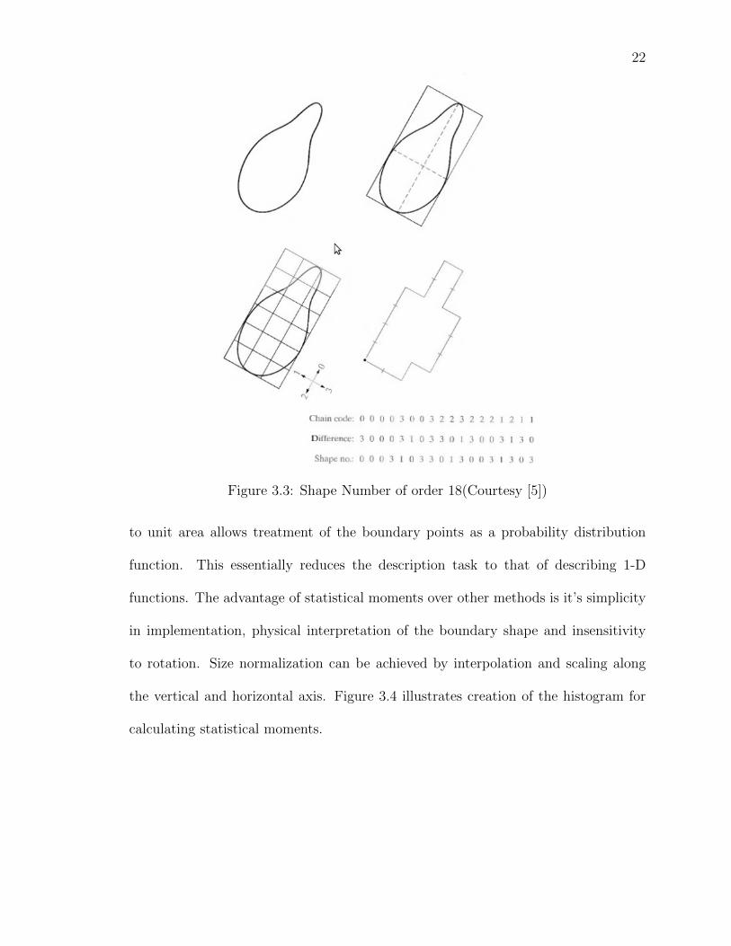
3.1.5 Shape Numbers
Shape number of a chain coded boundary based on a 4-connectivity directional
code is defined as the first difference of the smallest magnitude. The order n of a
shape number is defined as the number of digits required for representation. The first
difference is computed by treating the chain code as a circular sequence. An example
of a order 18 shape number is illustrated in Figure 3.3
3.1.6 Statistical Moments
Statistical moments for representing region boundaries is one of the more popular
methods for shape analysis and description. Boundary segments can be described
quantitatively by using simple statistical moments, such as mean, variance and higher
order statistical moments. A statistical moment is acquired for a boundary segment by
finding the end points of a boundary and rotating all boundary points in the segment
to align horizontally. This can be imagined as a histogram. Normalizing the histogram
22
Figure 3.3: Shape Number of order 18(Courtesy [5])
to unit area allows treatment of the boundary points as a probability distribution
function. This essentially reduces the description task to that of describing 1-D
functions. The advantage of statistical moments over other methods is it’s simplicity
in implementation, physical interpretation of the boundary shape and insensitivity
to rotation. Size normalization can be achieved by interpolation and scaling along
the vertical and horizontal axis. Figure 3.4 illustrates creation of the histogram for
calculating statistical moments.
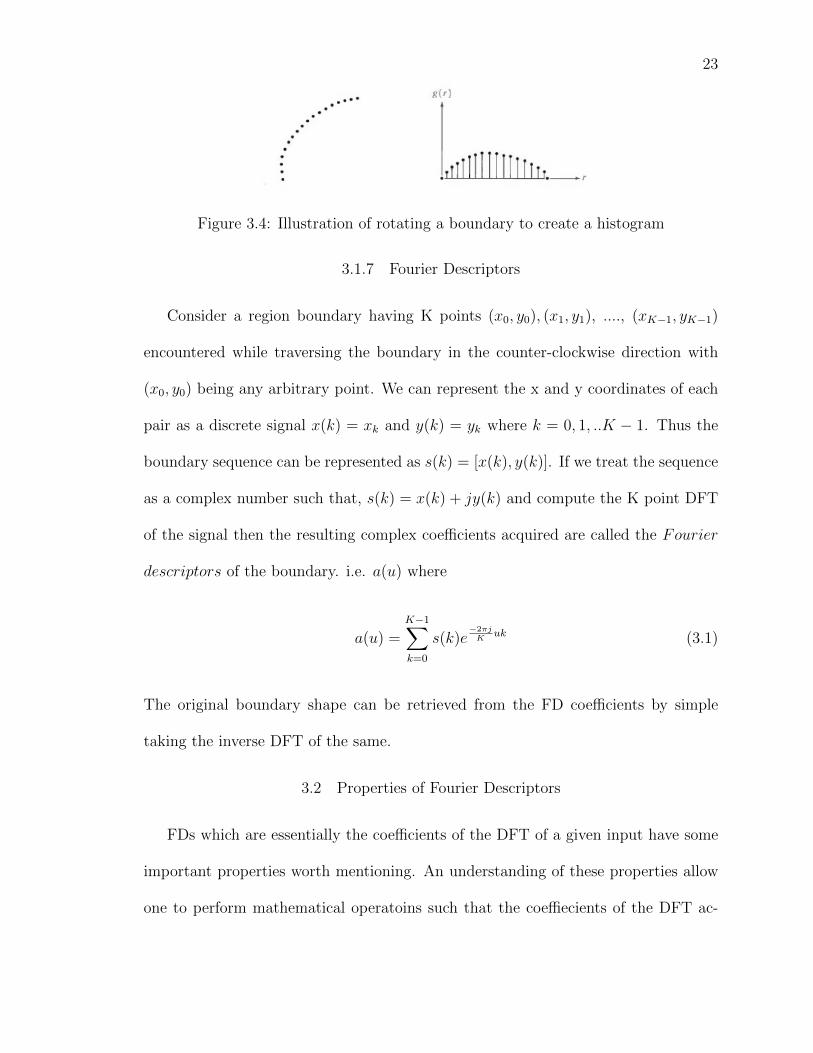
23
Figure 3.4: Illustration of rotating a boundary to create a histogram
3.1.7 Fourier Descriptors
Consider a region boundary having K points (x0, y0), (x1, y1), ...., (xK−1, yK−1)
encountered while traversing the boundary in the counter-clockwise direction with
(x0, y0) being any arbitrary point. We can represent the x and y coordinates of each
pair as a discrete signal x(k) = xk and y(k) = yk where k = 0, 1, ..K − 1. Thus the
boundary sequence can be represented as s(k) = [x(k), y(k)]. If we treat the sequence
as a complex number such that, s(k) = x(k) + jy(k) and compute the K point DFT
of the signal then the resulting complex coefficients acquired are called the Fourier
descriptors of the boundary. i.e. a(u) where
a(u) =K−1∑k=0
s(k)e−2πjK
uk (3.1)
The original boundary shape can be retrieved from the FD coefficients by simple
taking the inverse DFT of the same.
3.2 Properties of Fourier Descriptors
FDs which are essentially the coefficients of the DFT of a given input have some
important properties worth mentioning. An understanding of these properties allow
one to perform mathematical operatoins such that the coeffiecients of the DFT ac-

24
quired are invariant to changes in translation, orientation and scale. Some of the
important properties of FDs are discussed below. These properties and more are
detailed and readily proved in work by Oppenheim, A. V. and Schafer, R. W. [13]. If
x(n) is a input signal of finite length N and X(k) is the corresponding DFT obtained
using Equation 2.1, then,
1. Translation (circular shift) of the input signal by m units results in output being
multiplied by a linear phase as shown below
F{x(n−m)} = e−2πiN
kmX(k) (3.2)
2. Multiplying input x(n) by a linear phase e−2πiN
km would result in a circular shift
of the output frequencies
F{e2πiN
kmx(n)} = X(k −m) (3.3)
3. If the input x(n) is a real valued function, then the Fourier transform coefficients
of the outputX(k) are complex conjugates of the previous points mirrored about
the point X(N/2 + 1) (except X(0))
4. If the the input signal is contracted in the time domain then it results in an
expansion in the frequency output.
F{x(an)} =1
|a|X(k) (3.4)
5. Even if the real valued input signal x(n) is translated, the magnitude of the

25
coefficients of the Fourier Transform are left unchanged.
3.3 Techniques for generating Fourier Descriptors
The method described in Section 3.1.7 is not the only method for generating
the FDs of a given boundary signal. The work by Zhang, D. and Lu, G. in [22]
described three other techniques namely Centroid distance, Curvature Signature and
the Cumulative Angular Function to investigate results of classification using all four
selected techniques. In order to eliminate the effect of translation of the object within
the image, the Complex Co-ordinate technique is modified to remove the bias. This is
done by subtracting the centroid co-ordinate value from each of the boundary points
of the L point long boundary as illustrated in Equation 3.5
s(t) = [x(t)− xc] + j[y(t)− yc] (3.5)
where,
xc =1
L
L−1∑k=0
x(t) (3.6)
and
yc =1
L
L−1∑k=0
y(t) (3.7)
The centroid distance function, z(t), is in itself free of the bias of location (trans-
lation) of the object under observation. The centroid distance function is described
in Equation Zhang, D. and Lu, G.3.8
z(t) = ((x(t)− xc)2 + (y(t)− yc)2)1/2 (3.8)

26
The curvature function K(t), in which curvature represents the second derivative
of the boundary and first derivative of the boundary tangent function, is defined as
the differentiation of successive boundary angles calculated in a window w:
K(t) = θ(t)− θ(t− 1); (3.9)
where
θ(t) = arctan(y(t)− y(t− w)
x(t)− x(t− w)) (3.10)
The curvature function is inherently invariant to translation and rotation.
The curvature function defined previously contains discontinuities of size 2π since
the tangent angle function θ(t) can assume values between the interval [−ππ] or
[0, 2π]. Therefore, the cumulative angular function, ϕ(t), is defined as the net amount
of angular bend between the starting point z(0) and current position z(t) on the shape
boundary.
ϕ(t) = [θ(t)− θ(0)]mod(2π) (3.11)
A normalized/periodic cumulative angular function in a fixed direction can also be
defined as
ψ(t) = ϕ(L
2πt− t) (3.12)
After acquiring the FDs by using Equation 3.1 and any of the above mentioned
aligning techniques for the input signal, the FDs are conditioned inorder to obtain
translation, rotation and scaling invariance in the frequency domain. For FDs ob-
tained using complex co-ordinate alignment, all the N descriptors except the first one
(DC component), since it depends on the position of the object of interest, are needed

27
to index the shape. Therefore, it may be discarded. However, if the magnitude of
the remaining FDs is divided by the second component, scale invariance is obtained.
Thus, the invariant feature vector used to index the shape is then given by,
f = [|FD2||FD1|
,|FD3||FD1|
, ...,|FDN−1||FD1|
] (3.13)
For FDs generated using Equation 3.8 and 3.9, due to the alignment of the input and
the function being a real valued signal, only half of the frequencies are required to
represent the object. Scale invariance is obtained by dividing the magnitude values
of the first half of FDs by the DC component.
f = [|FD1||FD0|
,|FD2||FD0|
, ...,|FDN/2||FD0|
] (3.14)
FDs generated using the periodic cumulative function, which is also a real valued
function, are invariant to translation, rotation and scaling and can be used directly
for indexing the shape and only half the FDs are required to represent/index the
object of interest.
Shape normalization is done for all of the above mentioned techniques by sampling
the shape (boundary point co-ordinates, angle, etc.) at fixed intervals of θ.
3.4 Previous work on Fourier Descriptors
It should be noted that FDs have been used in research towards recognition of
objects in the past. In fact, literature has been published on FDs in 1967 by Blum
H.[3]. One of the old literatures found on the use of FDs for classifying different shapes
is by E. Persoon and K. Fu[15]. The work in this material was built upon the previous
28
work of Zahn, C. T. and Roskies, R. Z.[21] and Granlund, G. H.[6] and illustrated
the design, properties, advantages and disadvantages of each technique for generating
FDs. Experiments performed included, skeleton finding, character recognition and
machine part recognition using FDs, chain encoding and polygon approximation.
Results showed that FDs were the better method to use when identifying objects
whose boundaries are non-overlapping. Identification was carried out with translation,
rotation, scaling and addition of small quantities of random noise to the images of
the object classes.
The work done by Kuhl F. P. and Giardina C. R. [10] presented a direct method
for obtaining the Fourier coefficients of a chain coded contour and described a classi-
fication and recognition procedure applicable to classes of objects that cannot change
shape and whose images are subject to sensory equipment distortion. Advantages
of using this approach is that integration or the use of fast Fourier transform is not
required. Also, the bounds on accuracy, when using this procedure were proved to
be easy to specify. The elliptical properties of the FDs were discussed and used
for a convenient and intuitively pleasing procedure of normalizing a Fourier contour
representation.
The aim of the work by Harding, P. R. G. and Ellis, T. J. in[7] was to show
that using the FD on a set of trajectory data of hand gestures, it is possible to
recognize a range of pointing gestures that is invariant to natural variations due to
the single individual or a normal population. Fourier techniques were applied to the
data, appearence based co-ordinates of hand centroids and time steps normalized to a
fixed length by multirate techniques, to produce frequency domain data that is scale
and translation invariant. The results of inputting the complex harmonic data to
29
a Probabilistic Neural Network (PNN) for gesture classification were also discussed.
The PNN gave encouraging results at discriminating between pointing gestures with
90% accuracy.
In works performed by Zhang, D. and Lu, G. in [22], the objective was to build a
Java retrieval framework to compare shape retrieval using FDs derived from different
signatures. Common issues and techniques for shape representation and normaliza-
tion are also analyzed in the paper. All four shape signatures (boundary models)
were addressed namely (1) boundary point representation as a complex number, (2)
distance of boundary points from centroid, (3) curvature signature and (4) cumula-
tive angular function. Techniques for shape normalization and indexing of FDs for
each of the previously mentioned models were detailed. Experiments were conducted
in which a Java client-server framework is built to conduct a retrieval test. The re-
sults showed that shape retrieval using FDs derived from centroid distance signature
is significantly better than that using FDs derived from the other three signatures.
The property that centroid distance captures both local and global features of shape
makes it desirable as shape representation. It is robust and information preserving.
Although cumulative angular function has been used successfully for character recog-
nition, it was shown that it is not as robust as centroid distance in discriminating
general shapes. The curvature function was disqualified as a technique for retrieval
as it is extremely sensitive to noise and distortion. The use of curvature as shape
representation requires intensive boundary approximation to make it reliable.
A method for identifying human face profiles using FDs was proposed by Aibara,
T. and Ohue, K. and Oshita, Y. in their work [1]. This method was not subject to
conventional methods for face recognition. It was shown that the P-Fourier coefficients
30
in the low-frequency range are useful for human face profile recognition, that is, by
using 31 P-Fourier coefficients, a correct recognition rate of 93.1% for 130 subjects was
obtained. The procedure for extracting the open curve face profile included smoothing
using a gaussian filter, edge detection using a Sobel operator [13], binary valuation
of the profile image, thinning and finally 55 pixels upward and 90 pixels downward
from tip of the nose were used for pattern matching using the P-FDs obtained.
An informative paper that provided for an objective evaluation of the relative
performance of autoregressive and Fourier based methods was written by Kauppinen,
H. and Seppanen, T. and Pietikainen, M.[9]. The paper compared the performance
of the two techniques by performing non-occluded 2D boundary shape recognition on
two independent sets of data: images of airplanes and letters. For the purpose of per-
formance evaluation using Fourier based methods, four techniques were implemented
namely, curvature Fourier method, radius Fourier method, contour Fourier method
and A-Invariant method. For the purpose of performance evaluation using autore-
gressive methods, curvature autoregressive method, radius autoregressive method,
contour autoregressive method and CPARCOR method were implemented. Classifi-
cation tests were performed with 16, 32 and 64 samples from the boundary function
using a kNNs classifier with k set to 3. Results acquired from experiments performed
demonstrated that Fourier based methods outperformed autoregressive methods in
leave one out tests, while in the holdout tests autoregressive methods outperformed
Fourier based methods. This is justified since it is believed that autoregressive mod-
els are appropriate for modelling signals that have distinct modes in their frequency
spectrum. Whereas, Fourier based methods describe global geometric properties of
the object contours while autoregressive ones describe local properties.

31
An investigation of the problem in detecting and classifying moving objects in
image sequences from traffic scenes recorded with a static camera was performed in
the work by Kunttu, I. and Lepisto, L. and Rauhamaa, J. and Visa, A [11] . This
was done using a statistical, illumination invariant motion detection algorithm to
produce binary masks of changes in the scene. FDs of the shapes from the refined
masks are computed and used as feature vectors describing the different objects in
the scene. These FDs were then passed through a feedforward neural network to
distinguish between humans, vehicles, and background clutters. Images acquired
were passed through a homomorphic pre-filter and contextadaptive motion detection
system described in the paper which results in a binary motion mask. Using the
binary motion mask, the object candidates were labelled using a connected component
analysis. Boundary tracing was performed using a method introduced by Suzuki
and Ade in their work in [18] and the Freeman chain code was used to represent
it. Classification was tested using neural networks where complex FDs as well as
centroid FDs were used as feature vectors. From the results it was observed that
the traditional method worked equally well for both human and vehicle recognition,
which was not the case for the centroid based method.
Lastly, an introduction to the Fourier Series, the DFT, complex geometry and
FDs for shape analysis is provided in the technical report written by Skoglund K. [17]
for educational purpose. This report did not include any experiments or results. The
purpose of the literature was to describe in detail the use of Fourier analysis towards
it’s application to shape modelling and analysis.

CHAPTER 4: DESIGN AND TESTING
The design follows the standard design of a Artificial Intelligence (AI) machine.
The important blocks of the design are:
1. Sensing
2. Segmentation
3. Feature detection
4. Computational model (classifier)
5. Decision (inference)
The contribution of this work is towards step 3 of the AI machine. The first problem
statement is to create a new technique for generating FDs used for shape analysis and
representation using the error model of an ellipse fit to given data. The algorithm
dictated in Section 4.1 details the each block of the process. Two new techniques
are created which are identical, however in one technique shape normalization is not
performed which leads to non standard lengths of FDs. This is a drawback since one
cannot compare vectors which have different dimension. In order to compromise for
this drawback, a M -order polynomial is fit to the absolute value of the DFT and
the resulting coefficients of the polynomial are used as a feature vector. In the other
technique, shape normalization is performed and the FDs generated can be directly
used for classification. In Section 4.2 the process of testing the algorithm is detailed.
Testing in performed using the hardware and software mentioned in Sections 4.3 and
4.4.

33
4.1 Algorithm
Sensing: The process for generating the FD begins by acquisition of a 640x480
image using a planar imaging device. The image acquired is low pass filtered by
convolution with a 3x3 gaussian low pass filter. By doing so noise induced into the
image due to the inadequacies of the imaging device is reduced. The image is then
setup for segmentation.
Segmentation: A transformation from the RGB colorspace to grayscale may be
performed prior to segmentation. Using statistical analysis of the RGB components
of the image on may use the layer with the maximum standard deviation amongst the
pixels(contrast). During testing on the selected, color segmentation was performed
whereas the real time model of the algorithm used the only the layer with maximum
standard deviation for segmentation. In either case, we threshold and segment pixels
within the image which may have the same color value as the object of interest.
Nobuyuki Otsu’s work on histogram shape-based image thresholding [14] allows for
performing segmentation autonomously. Otsu’s algorithm is used for segmentation
as each image is analysed for the best range of gray level values to detail the object
of interest.
Feature detection(generation): Segmented pixels are grouped together to find
closed connected components. The area of each closed connected component, i.e.
total number of pixel in the closed connected component, is checked against a thresh-
old in order to eliminate components that are too small to be analysed. Boundary
extraction is then performed using dilation instead of erosion as mentioned in Equa-

34
tion 2.7. Therefore the extracted boundary is β(A), given by,
β(A) = (A⊕B)− A (4.1)
The length of the boundary is checked against a pre-determined threshold, usually
more than 360 pixels. If the length of the boundary does not meet the criteria, it
is discarded. The cartesian co-ordinates of each pixel on the selected boundary are
then extracted and the centroid of the boundary is calculated and subtracted from
each boundary point. This removes the effect of the bias of position of the object
within the image and the provides independence from translation. The boundary is
then converted to polar co-ordinates. Sampling is performed on the boundary such
that there is one pixel per degree change in the angle. The coordinate pairs are
reordered such that the boundary is sampled in either clockwise or counter-clockwise
manned. Sampling in a predetermined fashion ensures that a sequence is maintained.
The boundary co-ordinate system is then converted back to the cartesian system. An
ellipse is fit to the cartesian coordinates of the boundary. The elliptical fit reveals the
values for a and b which form the major and minor axes of the ellipse the best fits,
i.e. least square fit, the boundary co-ordinates. The equation of the ellipse is solved
for each co-ordinate pair of the boundary in order to obtain the normal distance of
the point from the fit ellipse.
e(r) =x2
a2+y2
b2− 1 (4.2)
The FDs are then obtained using Equation 3.1, the input to which is the error vector

35
e(r). Since e(r) is a real valued signal, property 5 holds true. We normalize each
of the FDs using Equation 3.14 which then forms the feature vector that is used
for classification. Rotation invariance is achieved since we use the magnitude of the
Fourier transform acquired which is independent of the starting point of the signal.
This is proved by property 1 of FDs and Equation 3.2 which shows that changing the
origin of a signal simply multiplies the signal with a linear phase there by changing
the phase of the output Fourier transform but does not cause a change in magnitude.
Hence a rotated object would still provide for the same FD as a non-rotated object.
Since we fit an ellipse to the segmented boundary, if the object is scaled, then the size
of the ellipse also changes and the error vector will remain proportional to objects
of a standard size. A flow chart illustrating the entire procedure is shown in Figures
4.1 and 4.2. Testing the proficiency of the aforementioned algorithm involved writing
programs for classifying a database of leaves. This provided a good standard to
measure performance of the newly designed technique against the earlier techniques.
[22] and [9] provided a comparison amongst the four techniques mentioned in Section
3.3 and proved that FDs obtained using curvature function and normalized/periodic
cumulative angular function are best if used for describing local features of a shape.

36
Figure 4.1: Flowchart for generating Fourier descriptors using the error model of an
elliptical fit to boundary points extracted(part 01)
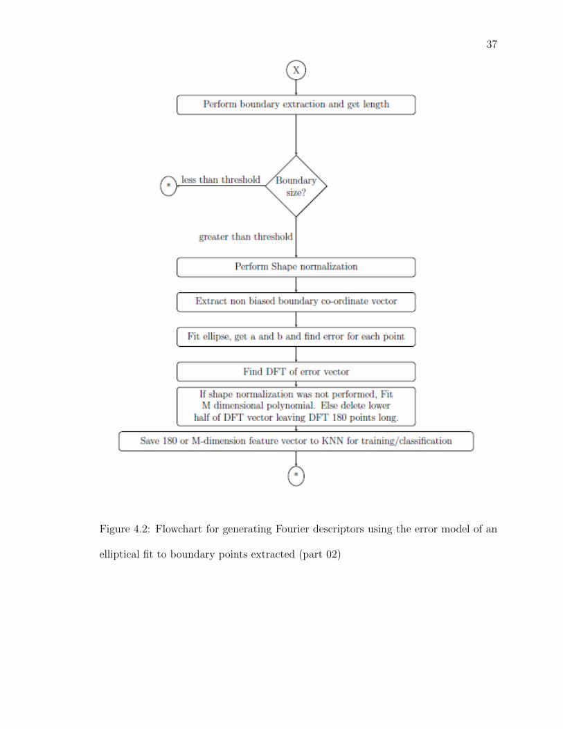
37
Figure 4.2: Flowchart for generating Fourier descriptors using the error model of an
elliptical fit to boundary points extracted (part 02)

38
4.2 Testing
As mentioned in Section 1.2 the purpose of this work is four fold. In order to
establish and investigate new methods for generating FDs, previous work on the same
was reviewed in Chapters 2 and 3. The technique described in this study is closely
related to what has been done in the past. Section 4.1 described the algorithm for
generating the FDs. The second part of the problem statement is to test the designed
algorithm on a database. Testing the technique is important as it allows to determine
variations in accuracy as compared to earlier techniques and predict behavior in real
time operation. It is to be noted that the technique like previous ones is dependent
on the segmentation and boundary extraction process through which the co-ordinates
of the boundary, which describe the shape of the boundary, are passed to the Fourier
transform for generation of FDs. Experiments conducted by Zhang, D. and Lu, G. in
[22] used a database of 95 binary images that represented synthetic polygon shapes
and bottle shapes respectively. The shapes in these images were transformed and
four similar shapes for each image were created using affine distortion, scaling and
rotation to expand the database to a total of 640 images. Only 16 shapes were used as
training images for the supervised learning algorithm to demonstrate the accuracy of
their designed retrieval system. In the case of this study, the database used by Zhang,
D. and Lu, G. [22] was not available. Therefore testing of the accuracy of the system
designed in this work was performed by classifying a database of 186 RGB colorspace
images of 3 types of leaves available at [20]. It should be noted that the problem of
classifying leaves is equally challenging as classification problem mentioned by Zhang,
D. and Lu, G. [22]. However, since the two databases are separate, experiments were
39
performed on the database of leaves using both the new technique and the older
ones. Results provided by these experiments would allow a better choice of technique,
amongst the two newly created, to be used for implementing the real time algorithm
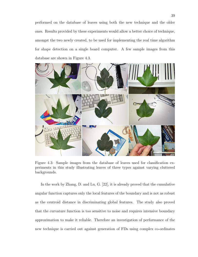
for shape detection on a single board computer. A few sample images from this
database are shown in Figure 4.3.
Figure 4.3: Sample images from the database of leaves used for classification ex-periments in this study illustrating leaves of three types against varying clutteredbackgrounds.
In the work by Zhang, D. and Lu, G. [22], it is already proved that the cumulative
angular function captures only the local features of the boundary and is not as robust
as the centroid distance in discriminating global features. The study also proved
that the curvature function is too sensitive to noise and requires intensive boundary
approximation to make it reliable. Therefore an investigation of performance of the
new technique is carried out against generation of FDs using complex co-ordinates

40
and centroid distance as we intend to discriminate using global features of an object.
To generate the FD, the boundary co-ordinates of the object of interest, in this
case the leaf, within the image must be extracted. This involves segmentation. Most
samples of leaves in the database are present in cluttered environment and conversion
from RGB to grayscale does not simplify segmentation. Hence, segmentation in color
is performed using preprocessing techniques mentioned in [19]. The leaf is extracted
using non-green background elimination in which the Red, Blue and Green component
channels of the image are first separated. An excess green index (ExG) and excess
red index (ExR) is calculated as,
ExG = 2×G−R−B (4.3)
and
ExR = 1.4×R−G−B (4.4)
Then the non-green background is eliminated by subtracting the excess red index
from the excess green index (ExG− ExR). As shown in Figure 4.5, one can clearly
see the boundary extracted after segmentation using the difference of the excess green
and excess red index. It should be noted however that the segmentation algorithm
used in this study does not always segment the correct object since the subject of
study, i.e. leaves, do not have a fixed color. An example where the segmentation
algorithm does not work is shown in Figure 4.6.
Once the leaf and the boundary are extracted as per the procedure mentioned
in the algorithm in section 4.1, an ellipse is fit to the cartesian co-ordinates of the
boundary with the bias of the centroid removed. For fitting the ellipse, an inbuilt

41
Figure 4.4: Database used by Zhang, D. and Lu, G.[22] for classification experimentsto compare success rates of different Fourier Descriptor techniques. This database wasnot available for the purpose of comparison. Therefore, experiments were performedon the leaves database shown in Figure4.3.
Figure 4.5: Segmentation using Otsu’s Algortihm and boundary extraction performedon the difference of excessive green and excessive red index.
Figure 4.6: Two example images that show failure in segmentation of the correctobject.

42
function in OpenCV called RotatedRect fitEllipse( const Mat& points ); is used.
This function uses a method similar to the one mentioned in Section 2.4. A complete
explanation on fitting ellipses to multidimensional data can be found in the works of
Gander, W., Golub, G. H. and Strebel, R. [4]. An example of an ellipse fit to the
boundary point co-ordinates is shown in Figure 4.7.
Experiments were performed with and without shape normalization. Shape nor-
malization involved sampling and saving cartesian coordinates of atleast one boundary
point per degree change in angle. The list of boundary point coordinates are then
treated as a discrete signal and are transformed using DFT to find the magnitude of
the resulting complex signal. Figures 4.8 and 4.9 show boundaries extracted with and
without shape normalization respectively. The FDs are obtained after normalizing
the acquired magnitude of DFT with the first coefficient of the magnitude of the
DFT signal as illustrated in Equation 3.14. If shape normalization is not performed,
different lengths of boundaries result in different lengths of the resultant signal after
performing DFT. These results cannot be used with a conventional classifier. Hence,
a M -order polynomial is fit to the absolute value of the DFT using least squares
fitting process and the values of the M coefficients obtained for the fit are used as the
features vector for the classifier. If shape normalization is performed, there is no need
to perform polynomial fitting and the 180 point FD feature vector can be directly
passed to the classifier for training or testing. The feature vector is 180 points long
since the fitting error signal is a real valued signal due to which property 5 of the FDs
holds true.
The computational model used in the case of this study is the kNNs classifier.
K-nearest neighbor classifier is a supervised learning algorithm where the result of

43
Figure 4.7: Example of an ellipse fit to boundary points extracted after segmentation.
Figure 4.8: Boundary of leaf extracted with no shape normalization. The Boundarycontains 1894 boundary points detailing fine variations of the boundary.
new instance query is classified based on majority of K-nearest neighbor category.
The purpose of this algorithm is to classify a new object based on attributes and
training samples. The classifiers do not use any model to fit and is purely based on
memory. Hence, it is a emperical classifier. Given a query point, it finds K number
of objects or (training points) closest to the query point. The distance of the query
point is evaluated against each training point in the memory by solving Equation
4.5.An inference is made based majority vote (consensus) among the label values of
the kNNs retrieved. K Nearest Neighbor algorithm used neighborhood classification

44
Figure 4.9: Boundary of leaf extracted with shape normalization and 360 boundarypoints. Shape normalization smooths out the boundary by sampling one boundarypoint per degree change in angle.
as the prediction value of the new query instance. This choice of classifier allows us to
use the similarity measurement system used in [22] by allowing K = 1. Finer details
regarding the kNN classifier may be found in the book by Bishop C. M.[2].
d = (M∑i=0
|fi − di|2)12 (4.5)
where f is the M dimensional query point and d is the M dimensional training point.
Additional testing was performed to check the variation in the performance of the
classifier when noise was added to the points sampled from the shape normalized
boundary. The noise was sampled from a normal distribution with zero mean and
different standard deviations and added to the radial value of the polar boundary
point. Higher values of standard deviations resulted in greater distortion of images.
Figure 4.10 shows a boundary plotted when radial gaussian noise was added to it. In
the case of testing in this study, radial gaussian noise with standard deviation 10 was
added to the boundary points extracted and classification tests were performed with

45
Figure 4.10: An example of Gaussian(normal) noise with zero mean and standarddeviation 10 added to boundary points. The upper row shows the original boundarypoints while the lower row shows the boundary points distorted due to addition ofnoise.
the noise added testing data and noise free training data.
4.3 Hardware Design
The experiments to determine the accuracy of the newly designed technique were
conducted on a Dell XPS laptop with:
• Processor: Intel Core 2 Duo T7250 / 2.0 GHz
• L2 Cache Memory: 2.0 MB
• Random Access Memory: 4GB DDR2 SDRAM - 667.0 MHz
• Graphics Processing Unit: nVidia Corporation G86 [GeForce 8400M GS]
46
• Video Memory: 128.0 MB
The real time implementation of the algorithm to identify an object of interest were
performed on a BeagleBoard-xM (BBxM) with the following technical specifications:
• Super-scalar ARM Cortex TM -A8
• 512-MB LPDDR RAM
• High-speed Universal Serial Bus (USB) 2.0 OTG port optionally powers the
board
• On-board four-port high-speed USB 2.0 hub with 10/100 Ethernet
• DVI-D (digital computer monitors and HDTVs)
• S-video (TV out)
• Stereo audio out/in
• High-capacity microSD slot and 4-GB microSD card
• JTAG
• Camera port
Image acquisition was performed using a ARK3188 single-chip PC camera having
specifications as follows:
• USB version 2.0 compliant specification for high-speed (480Mbps) and full-speed
(12Mbps) USB
• Support video data transfer in USB isochronous
• Complied with USB Video Class Version 1.1
• 8 Bit CMOS image raw data input
• Support VGA/1.3M CMOS sensor, such as Hynix 7131R, Omni Vision OV7670,
Micron MT9v011/MT9v111, PixelPlus PO3030 etc

47
• Up to 30fps@VGA or 10 [email protected] for PC mode video
• Provide individual R/G/B digital color gains control
• Provide snapshot function
• Embedded AE calculation and report
• Built-in gamma correction and auto white balance gain circuit
• Embedded high performance color processor
• JPEG baseline capability of compression encode
• No external memory needed
The object of interest in case of recognition was determined as Transcend JetFlash
300 USB Storage Device with size specifications 60mm x 18.8mm x 8.6mm
4.4 Software Design
The procedure for generating the FDs using the designed technique is independent
of any software package. However, to reproduce and verify the results mentioned in
Chapter 5 using the program code in the Appendix, it is advised to have a test system
with the following software packages installed:
1. Ubuntu 10.10 using a Linux 2.6.35-27-generic-pae kernel
2. Open Source Computer Vision Library version 2.2+ [8] and it’s dependencies.
3. Blob library for Computer Vision [12].
4. Database of images of leaves for testing the algorithm [20].
5. MATLAB for verifying computational results.
The real time system for testing the designed technique was built using the BeaglebBoard-
xM. This required bringing the development board to working standards i.e. install

48
a kernel and required packages for OpenCV. In order to install the kernel instruc-
tions detailed on “http://elinux.org/BeagleBoardUbuntu” were followed to install the
Maverick 10.10 distribution of Ubuntu. However, this is a extremely stripped down
version of Ubuntu without the presence of any compilers or packages to generate
executable binaries which are required to run to real time system. The following
commands were executed in sequence on the BBxM in order to install the required
packages for running OpenCV.
• apt-get upgrade -y
• apt-get -y install btrfs-tools i2c-tools nano pastebinit uboot-envtools uboot-
mkimage usbutils wget wireless-tools wpasupplicant linux-firmware devmem2
• apt-get install streamer –fix-missing
• apt-get install gcc
• apt-get install g++
• apt-get install gcj
• apt-get install build-essential
• apt-get install cmake
• apt-get install unrar python
• apt-get install build-essential python-yaml cmake subversion wget python-setuptools
mercurial
• apt-get install python-paramiko libgtest-dev python-numpy libboost1.42-all-dev
python-imaging libapr1-dev libbz2-dev pkg-config libaprutil1-dev python-dev
liblog4cxx10-dev

49
• apt-get install git
• apt-get install libncurses5-dev –fix-missing
• apt-get install ssh
• apt-get install vim
• apt-get install libxext-dev libavcodec-dev libavutil-dev libglut3-dev graphviz
libswscale-dev libavformat-dev libjasper-dev libgtk2.0-dev libgraphicsmagick++1-
dev
• apt-get install python-wxgtk2.8
• apt-get install libdc1394-22-dev –fix-missing
• apt-get install libv4l-dev
• apt-get install gstreamer0.10-plugins-base-apps
• apt-get install gstreamer0.10-ffmpeg
• apt-get install gfortran
• apt-get install doxygen
• apt-get install libgstreamer0.10-dev libgstreamer-plugins-base0.10-dev
Next, the OpenCV library was downloaded from [8], configured, made and installed
to the default directories within the Linux filesystem. Libraries installed included:
• libopencv calib3d.so
• libopencv contrib.so
• libopencv core.so
• libopencv features2d.so
• libopencv flann.so
• libopencv gpu.so

50
• libopencv highgui.so
• libopencv imgproc.so
• libopencv legacy.so
• libopencv ml.so
• libopencv objdetect.so
• libopencv video.so
After installing the packages and necessary libraries, the training modules and
classifier module programs were copied from the test system to the BBxM. The pro-
grams were compiled using the on-board gcc compiler.

CHAPTER 5: EVALUATION
A classifier can only be as good as the features that are used to train the model.
Therefore, for generating good features, one need to have a good feature detection
system. As mentioned before, the contribution of this work is towards creating an im-
proved version of the feature detection technique which uses FDs as features. Earlier
works used FDs which were generated using the four techniques mentioned in Section
3.3. Since cumulative angular function and the curvature function are not effective
in describing global features of objects as deduced by Zhang, D. and Lu, G. in [22],
they were not considered for the purpose of testing.
To compare the performance of classification using FDs generated from the error
model of an elliptical fit with and without shape normalization to the given plane
closed curve data against older techniques i.e. FDs generated by using the boundary
points as Complex Co-ordinates and Centroid distance, a classification experiment
was devised in which a database of 186 leaves were classified using a kNN classifier.
Performance was based on the number of correctly classified images for each class
of leaves. Four images from each class were chosen being a total twelve images being
used for training. While making the choice of training images it was assured that only
the leaf was segmented from the background. This was done inorder to ensure that
the classifier was not being trained with incorrect data due to incorrectly segmented
objects.
Results acquired from the process of classification are for each class(type) of leaf
52
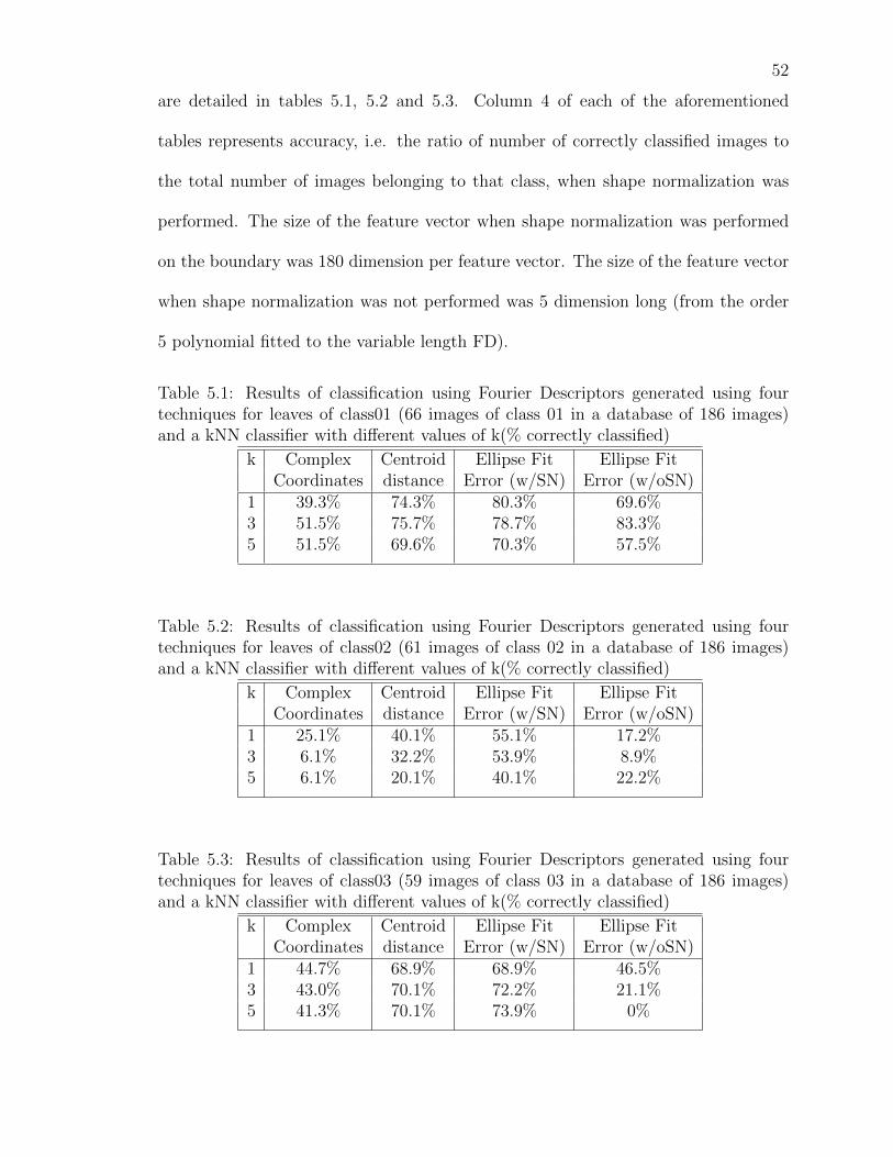
are detailed in tables 5.1, 5.2 and 5.3. Column 4 of each of the aforementioned
tables represents accuracy, i.e. the ratio of number of correctly classified images to
the total number of images belonging to that class, when shape normalization was
performed. The size of the feature vector when shape normalization was performed
on the boundary was 180 dimension per feature vector. The size of the feature vector
when shape normalization was not performed was 5 dimension long (from the order
5 polynomial fitted to the variable length FD).
Table 5.1: Results of classification using Fourier Descriptors generated using fourtechniques for leaves of class01 (66 images of class 01 in a database of 186 images)and a kNN classifier with different values of k(% correctly classified)
k Complex Centroid Ellipse Fit Ellipse FitCoordinates distance Error (w/SN) Error (w/oSN)
1 39.3% 74.3% 80.3% 69.6%3 51.5% 75.7% 78.7% 83.3%5 51.5% 69.6% 70.3% 57.5%
Table 5.2: Results of classification using Fourier Descriptors generated using fourtechniques for leaves of class02 (61 images of class 02 in a database of 186 images)and a kNN classifier with different values of k(% correctly classified)
k Complex Centroid Ellipse Fit Ellipse FitCoordinates distance Error (w/SN) Error (w/oSN)
1 25.1% 40.1% 55.1% 17.2%3 6.1% 32.2% 53.9% 8.9%5 6.1% 20.1% 40.1% 22.2%
Table 5.3: Results of classification using Fourier Descriptors generated using fourtechniques for leaves of class03 (59 images of class 03 in a database of 186 images)and a kNN classifier with different values of k(% correctly classified)
k Complex Centroid Ellipse Fit Ellipse FitCoordinates distance Error (w/SN) Error (w/oSN)
1 44.7% 68.9% 68.9% 46.5%3 43.0% 70.1% 72.2% 21.1%5 41.3% 70.1% 73.9% 0%

53
These results indicate that FDs generated using the error model of an ellipse fit
to the data with shape normalization have a higher accuracy in correctly classifying
the object of interest. It consistently works better, since we do not see a single case of
reduction in accuracy as compared to earlier techniques. When the value of k, i.e. the
number of nearest neighbours which participate in voting the output, is changed, a
reduction in accuracy is observed in some cases. This is however due to the emperical
nature of the data input to the classifier. In the case when FDs are generated without
using shape normalization, the accuracy of the classification process is not guaranteed
as compared to older techniques which is a major drawback.
Table 5.4: Average time required for calculation of the Fourier Descriptors on apersonal computing machine as described in section 4.3
Technique Average Time (milliseconds)
Complex co-ordinates 35Centroid distace 35Ellipse Fit error w/ SN 37Ellipse Fit error w/o SN 37
In order to prove the robustness against noise, classification tests were performed
by adding noise to the testing data of each class. Tables 5.5, 5.6 and 5.7 illustrate the
results acquired from the testing. These results readily show that there is a massive
drop in accuracy. This is expected since the testing data itself is being corrupted.
However, as compared to FDs generated using complex co-ordinates and centroid
distance, the classification accuracy of FDs generated using fit error of an ellipse is
found to be relatively higher in two out of the three classes available. The accuracy is
reduced by half whereas for the other two techniques it is reduced to much less than
half the original accuracy when noise was not present in the testing data.
These results illustrate the improvement of the new technique over conventional

54
Table 5.5: Results of classification using Fourier Descriptors generated using threetechniques for leaves of class01 (66 images of class 01 in a database of 186 images)when noise is added to the testing data(% correctly classified)
k Complex Centroid Ellipse FitCoordinates distance Error (w/SN)
1 37.8% 1.5% 40.9%3 53.0% 3.0% 37.8%5 53.0% 4.5% 42.4%
Table 5.6: Results of classification using Fourier Descriptors generated using complexco-ordinates system for leaves of class02 (61 images of class 02 in a database of 186images) when noise is added to the testing data(% correctly classified)
k Complex Centroid Ellipse FitCoordinates distance Error (w/SN)
1 20.6% 58.9% 22.2%3 0.6% 52.2% 27.2%5 0.6% 52.2% 27.2%
techniques in terms of accuracy and reliability. This encouraged the development of
a real time recognition system using a simple web camera and an embedded devel-
opment board, the BBxM. Codes mentioned in APPENDIX A.2 were modified to
create a module for generating FDs using the error model of an elliptical fit to the
boundary data of plane closed objects and saving these features extracted from the
training image. The features were saved into a “yml” file format used by OpenCV
using a FileStorage object. Another module was developed which trained a kNN
classifier object available in OpenCV Machine Learning (libopencv ml.so) library us-
ing the previously saved file “feature data.yml”. After training the classifier, the
module opened a stream from the attached web camera. The program was looped to
query frames from the imaging device, segment the image, find the segmented object
having the largest boundary and generate it’s FD using the designed technique. The
FD of the acquired image is then directly input to the classifier for evaluation of the
55
Table 5.7: Results of classification using Fourier Descriptors generated using complexco-ordinates system for leaves of class03 (59 images of class 03 in a database of 186images) when noise is added to the testing data(% correctly classified)
k Complex Centroid Ellipse FitCoordinates distance Error (w/SN)
1 24.4% 41.3% 61.7%3 43.1% 34.6% 46.4%5 38.1% 38.1% 32.9%
label to be assigned. For the purpose of training only one image per class of object
was used. The three images used for training are shown in Figures 5.1, 5.2 and 5.3.
Some of the images captured during realtime operation of the system are shown in
Figures 5.4, 5.5 and 5.6.
Figure 5.1: Offline training images, object class 01.
Figure 5.2: Offline training images, object class 02.

56
Figure 5.3: Offline training images, object class 03.
Figure 5.4: Real time capture and recognition, object class 01.
Figure 5.5: Real time capture and recognition, object class 02.
Figure 5.6: Real time capture and recognition, object class 03.
It should be noted that the system is susceptible to failure when the segmentation
algorithm fails. As shown in Figure A.2, when Otsu’s segmentation fails to capture
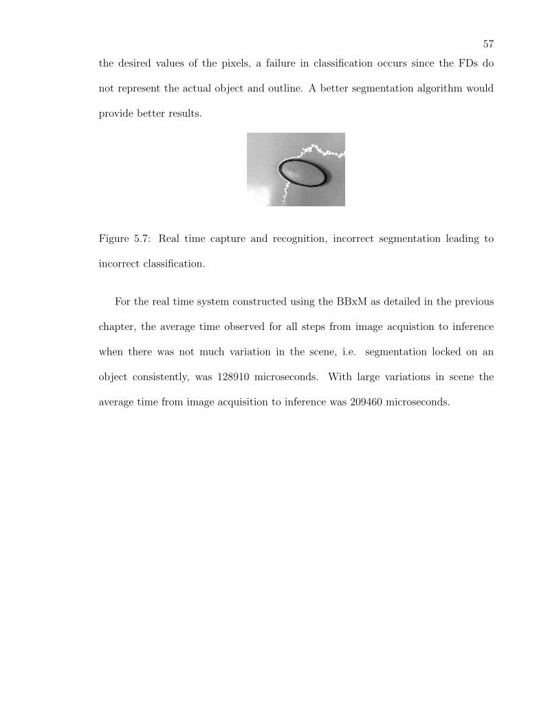
57
the desired values of the pixels, a failure in classification occurs since the FDs do
not represent the actual object and outline. A better segmentation algorithm would
provide better results.
Figure 5.7: Real time capture and recognition, incorrect segmentation leading to
incorrect classification.
For the real time system constructed using the BBxM as detailed in the previous
chapter, the average time observed for all steps from image acquistion to inference
when there was not much variation in the scene, i.e. segmentation locked on an
object consistently, was 128910 microseconds. With large variations in scene the
average time from image acquisition to inference was 209460 microseconds.

CHAPTER 6: CONCLUSION
The goals of this thesis were achieved which included the designing and inves-
tigation of a new technique for generating feature vectors which can be input to a
classifier for purpose of recognition. This technique used the error model of an ellipse
fit to the co-ordinates of the shape normalized data points. Experiments were per-
formed to investigate the accuracy of recognition using FDs generated using the error
model of an elliptical fit to the given data against old techniques i.e. FDs generated
using the data as complex co-ordinates and centroid distance. A real time system
was developed to perform recognition of objects using the designed algorithm using
BBxM and the performance of the real time system was evaluated.
From the experiments performed on a database of leaves consisting of three classes
of leaves, it was found that this new technique provided for consistently higher ac-
curacy rates when used for classification as compared to older techniques that used
complex co-ordinate and centroid distance systems to generate the FDs. It was de-
duced that shape normalization was an essential part of the technique since the second
technique investigated, which did not use shape normalization failed to provide con-
sistent recognition rates. The results also proved that the technique is invariant to
translation, rotation and scaling of the objects of interest. Tests for robustness against
noise also proved that FDs generated using the error model of the fit ellipse are much
more accurate than FDs generated using centroid distance or complex co-ordinate
systems.

59
These results encouraged the development of a real time system for detecting
objects of interest using FDs generated using an error model of an ellipse fit to plane
closed curves within images and using them for recognition on robotic vehicles. This
work can be directly incorporated into robotic applications which involve detecting
objects using an overhead camera. The work can also be used as it is in robotic arm
systems which need a form of visual recognition that is invariant to the pose of the
object of interest. The work can also be modified for other works such as aircraft
and vehicle recognition from an aerial camera. The real time program module can be
directly incorporated as a node into the Robot Operating System (ROS) framework
which has gained popularity in recent years. This is essential a virtue of having
the programs written using the OpenCV library which is also a part of the ROS
framework.
Future work using this new technique for should look forward to fusion of texture
based recognition alongside this technique which is based on global shape features.
Another area of investigation would be to use the technique developed in this work
for detection of partially occluded objects and extension towards three dimensional
recognition. Another interesting application could look into the possibility of map-
ping using this technique, for e.g. train the classifier with multiple planar images of
different locations(rooms) within a map(building) and perform real time testing to
find the current location of the camera within the map.

60
BIBLIOGRAPHY
[1] T. Aibara, K. Ohue, and Y. Oshita. Human face profile recognition by a P-Fourier descriptor. Optical Engineering, 32:861–863, April 1993.
[2] C. M. Bishop. Pattern Recognition and Machine Learning (Information Scienceand Statistics). Springer-Verlag New York, Inc., Secaucus, NJ, USA, 2006.
[3] H. Blum. A Transformation for Extracting New Descriptors of Shape. In WeiantWathen-Dunn, editor, Models for the Perception of Speech and Visual Form,pages 362–380. MIT Press, Cambridge, 1967.
[4] W. Gander, G. H. Golub, and R. Strebel. Least-squares fitting of circles andellipses. BIT Numerical Mathematics, 34:558–578, 1994. 10.1007/BF01934268.
[5] R. C. Gonzalez and R. E. Woods. Digital Image Processing. Addison-WesleyLongman Publishing Co., Inc., Boston, MA, USA, 2nd edition, 2001.
[6] G. H. Granlund. Fourier preprocessing for hand print character recognition.IEEE Trans. Comput., 21:195–201, February 1972.
[7] P. R. G. Harding and T. J. Ellis. Recognizing hand gesture using fourier descrip-tors. In Proceedings of the Pattern Recognition, 17th International Conferenceon (ICPR’04) Volume 3 - Volume 03, ICPR ’04, pages 286–289, Washington,DC, USA, 2004. IEEE Computer Society.
[8] Intel. Open source computer vision library v2.2.http://opencv.willowgarage.com/wiki/, December 2010.
[9] H. Kauppinen, T. Seppanen, and M. Pietikainen. An experimental comparisonof autoregressive and fourier-based descriptors in 2d shape classification. IEEETrans. Pattern Anal. Mach. Intell., 17:201–207, February 1995.
[10] F. P. Kuhl and C. R. Giardina. Elliptic fourier features of a closed contour.Computer Graphics and Image Processing, 18(3):236 – 258, 1982.
[11] I. Kunttu, L. Lepisto, J. Rauhamaa, and A. Visa. Multiscale fourier descriptorfor shape classification. In Proceedings of the 12th International Conference onImage Analysis and Processing, pages 536–, Washington, DC, USA, 2003. IEEEComputer Society.
[12] C. C. Linan. Blob library for opencv. http://code.google.com/p/cvblob/, June2011.
[13] A. V. Oppenheim and R. W. Schafer. Discrete-time signal processing. Prentice-Hall, Inc., Upper Saddle River, NJ, USA, 1989.
[14] N. Otsu. A threshold selection method from gray-level histograms. Systems,Man and Cybernetics, IEEE Transactions on, 9(1):62 –66, January 1979.

61
[15] E. Persoon and K. Fu. Shape discrimination using fourier descriptors. IEEETransactions on Systems, Man, and Cybernetics, 7:170–179, 1977.
[16] O. Raut. Polyfit function for open source computer vision library.https://code.ros.org/trac/opencv/ticket/1124, Dec 2010.
[17] K. Skoglund. Fourier series, the DFT and shape modelling. Technical report, In-formatics and Mathematical Modelling, Technical University of Denmark, DTU,Richard Petersens Plads, Building 321, DK-2800 Kgs. Lyngby, October 2004.
[18] S. Suzuki and K. Be. Topological structural analysis of digitized binary imagesby border following. Computer Vision, Graphics, and Image Processing, 30(1):32– 46, 1985.
[19] X. Tang, M. Liu, H. Zhao, and W. Tao. Leaf extraction from complicatedbackground. In Image and Signal Processing, 2009. CISP ’09. 2nd InternationalCongress on, pages 1 –5, October 2009.
[20] M. Weber. 186 images of leaves against different backgrounds.http://www.vision.caltech.edu/html-files/archive.html, April 2003.
[21] C. T. Zahn and R. Z. Roskies. Fourier Descriptors for Plane Closed Curves.Transactions on Computers, IEEE, c-21(3):269–281, March 1972.
[22] D. Zhang and G. Lu. A comparative study on shape retrieval using fourierdescriptors with different shape signatures. Victoria, 14(1):19, 2001.

62
APPENDIX A: SOURCE CODE
The following list the code and project structures for image acquisition, training
the classifier and testing the classifier. All code was written in C++.
A.1 Project Structures
The following two Figures illustrate the structure of the training module and
classification module for testing the algorithm.
Figure A.1: Training Module Project Structure.

63
Figure A.2: Classification Module Project Structure.

64
A.2 Program codes
Source/cvPolyfit.hpp
/∗
∗ c vPo l y f i t . hpp
∗
∗ Created on : Jun 6 , 2011
∗ Author : Onkar Raut
∗/
#ifndef CVPOLYFIT HPP
#define CVPOLYFIT HPP
void c vPo l y f i t ( cv : : Mat &src x , cv : : Mat &src y , cv : : Mat &dst , int order ) ;
#endif /∗ CVPOLYFIT HPP ∗/
Source/cvPolyfit.cpp
/∗
∗ c vPo l y f i t . hpp
∗
∗ Created on : Jun 6 , 2011
∗ Author : Onkar Raut
∗/
#include <opencv/cv . h>
#include <opencv/ h ighgu i . h>
#include ” cvPo l y f i t . hpp”
using namespace cv ;
void c vPo l y f i t ( cv : : Mat &src x , cv : : Mat &src y , cv : : Mat &dst , int order )
{
CVFUNCNAME(” cvPo l y f i t ” ) ;
CV BEGIN ;
{
CV ASSERT(( s r c x . rows>0)
&&(( int ) s r c y . rows>0)
&&(( int ) s r c x . c o l s==1)
&&(s r c y . c o l s==1)

65
&&(dst . c o l s==1)
&&(dst . rows==(order +1))
&&(( int ) order >=1));
Mat X;
X = Mat : : z e r o s ( s r c x . rows , order+1,CV 32FC1 ) ;
Mat copy ;
for ( int i = 0 ; i <=order ; i++)
{
copy = s r c x . c l one ( ) ;
pow( copy , i , copy ) ;
Mat M1 = X. co l ( i ) ;
copy . c o l ( 0 ) . copyTo (M1) ;
}
Mat X t , X inv ;
t ranspose (X, X t ) ;
Mat temp = X t∗X;
Mat temp2 ;
i nv e r t ( temp , temp2 ) ;
Mat temp3 = temp2∗X t ;
Mat W = temp3∗ s r c y ;
#ifdef DEBUG
cout<<”PRINTING INPUT AND OUTPUT FOR VALIDATION AGAINST MATLAB RESULTS\n” ;
cout<<”SRC X: ”<<s r c x<<endl ;
cout<<”SRC Y: ”<<s r c y<<endl ;
cout<<”X: ”<<X<<endl ;
cout<<”X T : ”<<X t<<endl ;
cout<<”W: ”<<W<<endl ;
#endif
dst = W. c lone ( ) ;
}
CV END ;
}

66
Source/main equal interval.cpp
/∗
∗ main . cpp
∗
∗ Created on : Jun 23 , 2011
∗ Author : Onkar Raut
∗ Purpose : Performs segmentat ion on l e a v e s f o r g iven images and c r ea t e s
∗ a f ea tu r e vec tor c on s i s t i n g o f Fourier Descr ip tor s us ing one o f
∗ the t echn iques COMPLEX COORDINATES, CENTROID DISTANCE or FIT ERROR
∗ o f an e l l i p s e .
∗ Usage : <name of this program> <path to image database> <number of images>
∗ <image sequence heading>
∗/
#define RENDER
#define VERIFY ANGLE
//#de f ine USE COMPLEX COORDINATES
//#de f ine USE CENTROID DISTANCE
#define USE FIT ERROR
#ifdef USE COMPLEX COORDINATES
#undef USE CENTROID DISTANCE
#undef USE FIT ERROR
#endif
#i fde f USE CENTROID DISTANCE
#undef USE COMPLEX COORDINATES
#undef USE FIT ERROR
#endif
#i fde f USE FIT ERROR
#undef USE COMPLEX COORDINATES
#undef USE CENTROID DISTANCE
#endif

67
#ifndef USECOMMANDLINE
#define NUM TRAINING IMAGES (66)
#endif
#define PI (M PI)
#define DFT LENGTH (360)
#include <opencv/cv . h>
#include <opencv/ h ighgu i . h>
#include ” cvPo l y f i t . hpp”
#include <iostream>
#include <math . h>
using namespace cv ;
using namespace std ;
F i l eS to rag e f s ( ” t e s t d a t a . yml” , F i l eS to rag e : :WRITE) ;
#ifdef USE COMPLEX COORDINATES
Mat f e a t u r e v e c t o r (DFT LENGTH−1,NUM TRAINING IMAGES,CV 32FC1 ) ;
Mat f i n a l f e a t u r e v e c t o r (NUM TRAINING IMAGES,DFT LENGTH−1,CV 32FC1 ) ;
#endif
#i fde f USE CENTROID DISTANCE
Mat f e a t u r e v e c t o r (DFT LENGTH−1,NUM TRAINING IMAGES,CV 32FC1 ) ;
Mat f i n a l f e a t u r e v e c t o r (NUM TRAINING IMAGES,DFT LENGTH−1,CV 32FC1 ) ;
#endif
#i fde f USE FIT ERROR
Mat f e a t u r e v e c t o r (DFT LENGTH−1,NUM TRAINING IMAGES,CV 32FC1 ) ;
Mat f i n a l f e a t u r e v e c t o r (NUM TRAINING IMAGES,DFT LENGTH−1,CV 32FC1 ) ;
#endif
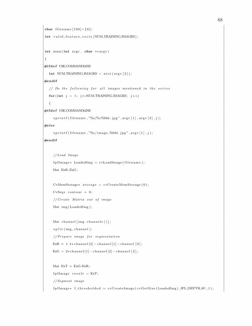
68
char f i l ename [100 ]={0} ;
int v a l i d f e a t u r e v e c t s [NUM TRAINING IMAGES ] ;
int main ( int argc , char ∗∗ argv )
{
#ifdef USECOMMANDLINE
int NUM TRAINING IMAGES = ato i ( argv [ 2 ] ) ;
#endif
// Do the f o l l ow i n g f o r a l l images mentioned in the s e r i e s
for ( int j = 1 ; j<=NUM TRAINING IMAGES; j++)
{
#ifdef USECOMMANDLINE
s p r i n t f ( f i l ename , ”%s/%s%04d . jpg ” , argv [ 1 ] , argv [ 3 ] , j ) ;
#else
s p r i n t f ( f i l ename , ”%s/ image %04d . jpg ” , argv [ 1 ] , j ) ;
#endif
//Load Image
IplImage ∗ LoadedImg = cvLoadImage ( f i l ename ) ;
Mat ExR,ExG;
CvMemStorage∗ s t o rage = cvCreateMemStorage ( 0 ) ;
CvSeq∗ contour = 0 ;
//Create Matrix out o f image
Mat img (LoadedImg ) ;
Mat channel [ img . channe l s ( ) ] ;
s p l i t ( img , channel ) ;
//Prepare image fo r segmentat ion
ExR = 1.4∗ channel [2]− channel [1]− channel [ 0 ] ;
ExG = 2∗ channel [1]− channel [2]− channel [ 2 ] ;
Mat ExT = ExG−ExR;
IplImage r e s u l t = ExT;
//Segment image
IplImage ∗ I t h r e sho l d ed = cvCreateImage ( cvGetSize ( LoadedImg ) , IPL DEPTH 8U , 1 ) ;
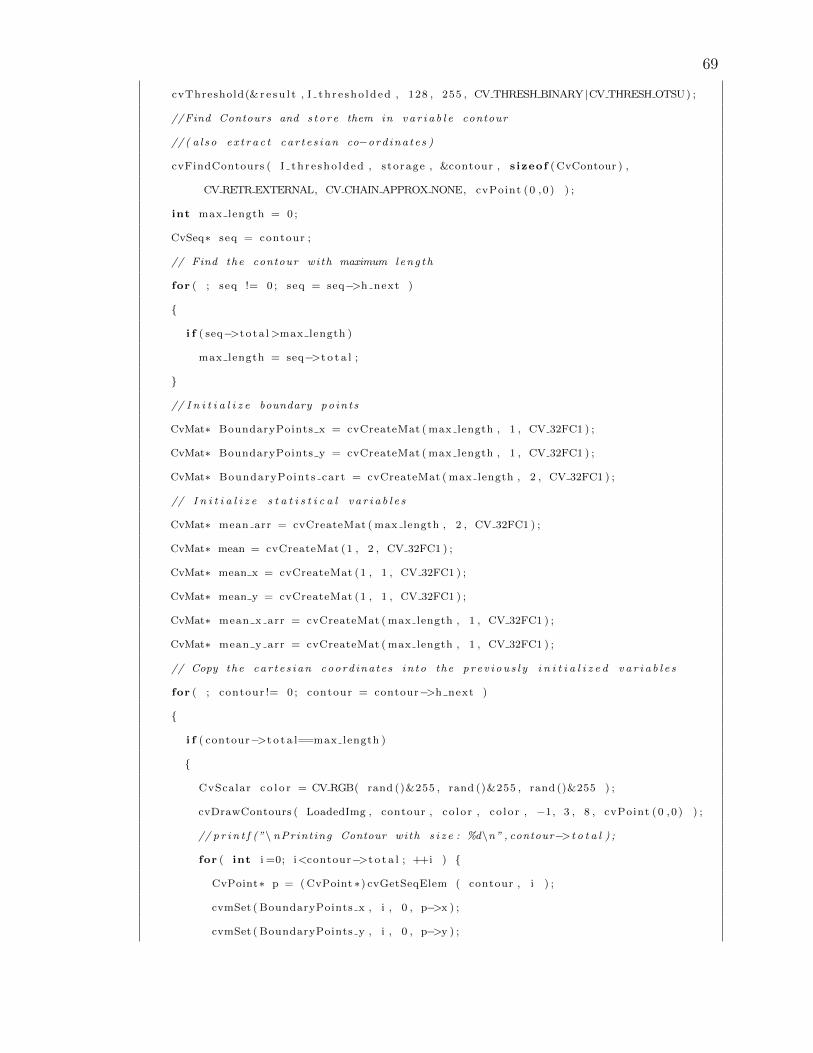
69
cvThreshold(& r e su l t , I th r e sho lded , 128 , 255 , CV THRESH BINARY |CV THRESH OTSU) ;
//Find Contours and s t o r e them in v a r i a b l e contour
// ( a l s o e x t r a c t ca r t e s i an co−ord ina t e s )
cvFindContours ( I th r e sho lded , s torage , &contour , s izeof (CvContour ) ,
CV RETR EXTERNAL, CV CHAIN APPROX NONE, cvPoint (0 , 0 ) ) ;
int max length = 0 ;
CvSeq∗ seq = contour ;
// Find the contour with maximum leng t h
for ( ; seq != 0 ; seq = seq−>h next )
{
i f ( seq−>t o ta l>max length )
max length = seq−>t o t a l ;
}
// I n i t i a l i z e boundary po in t s
CvMat∗ BoundaryPoints x = cvCreateMat ( max length , 1 , CV 32FC1 ) ;
CvMat∗ BoundaryPoints y = cvCreateMat ( max length , 1 , CV 32FC1 ) ;
CvMat∗ BoundaryPoints cart = cvCreateMat ( max length , 2 , CV 32FC1 ) ;
// I n i t i a l i z e s t a t i s t i c a l v a r i a b l e s
CvMat∗ mean arr = cvCreateMat ( max length , 2 , CV 32FC1 ) ;
CvMat∗ mean = cvCreateMat (1 , 2 , CV 32FC1 ) ;
CvMat∗ mean x = cvCreateMat (1 , 1 , CV 32FC1 ) ;
CvMat∗ mean y = cvCreateMat (1 , 1 , CV 32FC1 ) ;
CvMat∗ mean x arr = cvCreateMat ( max length , 1 , CV 32FC1 ) ;
CvMat∗ mean y arr = cvCreateMat ( max length , 1 , CV 32FC1 ) ;
// Copy the ca r t e s i an coord ina te s in to the p r e v i ou s l y i n i t i a l i z e d v a r i a b l e s
for ( ; contour != 0 ; contour = contour−>h next )
{
i f ( contour−>t o t a l==max length )
{
CvScalar c o l o r = CV RGB( rand ()&255 , rand ()&255 , rand ()&255 ) ;
cvDrawContours ( LoadedImg , contour , co lo r , co lo r , −1, 3 , 8 , cvPoint (0 , 0 ) ) ;
// p r i n t f (”\ nPrint ing Contour with s i z e : %d\n” , contour−>t o t a l ) ;
for ( int i =0; i<contour−>t o t a l ; ++i ) {
CvPoint∗ p = (CvPoint ∗) cvGetSeqElem ( contour , i ) ;
cvmSet ( BoundaryPoints x , i , 0 , p−>x ) ;
cvmSet ( BoundaryPoints y , i , 0 , p−>y ) ;

70
cvmSet ( BoundaryPoints cart , i , 0 , p−>x ) ;
cvmSet ( BoundaryPoints cart , i , 1 , p−>y ) ;
}
}
}
// Ca l cu la t e mean( cen t ro id ) f o r the contour
cvReduce ( BoundaryPoints cart ,mean , 0 , CV REDUCEAVG) ;
cvReduce ( BoundaryPoints x , mean x , 0 , CV REDUCEAVG) ;
cvReduce ( BoundaryPoints y , mean y , 0 , CV REDUCEAVG) ;
cvRepeat (mean , mean arr ) ;
cvRepeat (mean x , mean x arr ) ;
cvRepeat (mean y , mean y arr ) ;
// Remove e f f e c t o f cen t ro id from the contour
cvSub ( BoundaryPoints cart , mean arr , BoundaryPoints cart ) ;
cvSub ( BoundaryPoints x , mean x arr , BoundaryPoints x ) ;
cvSub ( BoundaryPoints y , mean x arr , BoundaryPoints y ) ;
// Prepare to send the co−ord ina t e s f o r f i t t i n g an e l l i p s e
Mat po in t s = BoundaryPoints cart ;
#ifdef VERIFY ANGLE
//Convert to Polar f o r sampling
Mat po la r ( max length , 2 ,CV 32FC1 ) ;
Mat M1 = po la r . c o l ( 0 ) ;
Mat M2 = po la r . c o l ( 1 ) ;
cartToPolar ( po in t s . c o l ( 0 ) , po in t s . c o l ( 1 ) ,M1,M2) ;
#endif
Mat sampled po ints (DFT LENGTH,2 ,CV 32FC1 ) ;
int counter = 0 ;
for ( f loat ang le = 0 ; angle<=2∗PI ; ang le = angle+PI /180)
{
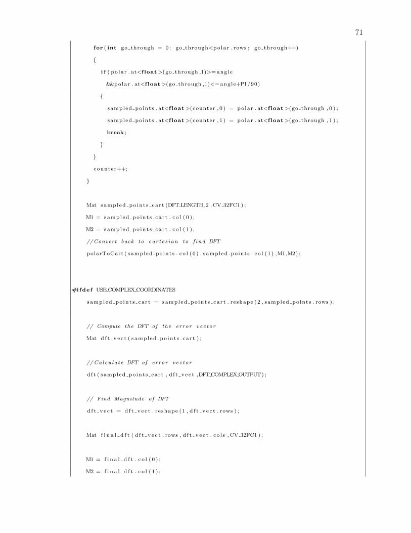
71
for ( int go through = 0 ; go through<po la r . rows ; go through++)
{
i f ( po la r . at<f loat>(go through ,1)>=angle
&&po la r . at<f loat>(go through ,1)<=angle+PI /90)
{
sampled po ints . at<f loat>(counter , 0 ) = po la r . at<f loat>(go through , 0 ) ;
sampled po ints . at<f loat>(counter , 1 ) = po la r . at<f loat>(go through , 1 ) ;
break ;
}
}
counter++;
}
Mat samp l ed po in t s ca r t (DFT LENGTH,2 ,CV 32FC1 ) ;
M1 = samp l ed po in t s ca r t . c o l ( 0 ) ;
M2 = samp l ed po in t s ca r t . c o l ( 1 ) ;
//Convert back to ca r t e s i an to f i nd DFT
polarToCart ( sampled po ints . c o l ( 0 ) , sampled po ints . c o l ( 1 ) ,M1,M2) ;
#ifdef USE COMPLEX COORDINATES
samp l ed po in t s ca r t = samp l ed po in t s ca r t . reshape (2 , sampled po ints . rows ) ;
// Compute the DFT of the error vec to r
Mat d f t v e c t ( s amp l ed po in t s ca r t ) ;
// Ca l cu la t e DFT of error vec tor
d f t ( sampled po in t s ca r t , d f t v e c t ,DFTCOMPLEXOUTPUT) ;
// Find Magnitude o f DFT
d f t v e c t = d f t v e c t . reshape (1 , d f t v e c t . rows ) ;
Mat f i n a l d f t ( d f t v e c t . rows , d f t v e c t . co l s , CV 32FC1 ) ;
M1 = f i n a l d f t . c o l ( 0 ) ;
M2 = f i n a l d f t . c o l ( 1 ) ;

72
// Get Fourier Descr ip tor
cartToPolar ( d f t v e c t . c o l ( 0 ) , d f t v e c t . c o l ( 1 ) ,M1,M2) ;
M1 = M1 / M1. at<f loat > (0 ,0) ;
//Save Fourier Descr ip tor as f e a t u r e
Mat temp = f e a t u r e v e c t o r . c o l ( j −1);
M1. rowRange (1 ,M1. rows ) . copyTo ( temp ) ;
#endif
#i fde f USE CENTROID DISTANCE
Mat c en t r o i d d i s t a n c e = sampled po ints . c o l ( 0 ) ;
// Compute the DFT of the error vec to r
Mat d f t v e c t ( c e n t r o i d d i s t a n c e ) ;
// Ca l cu la t e DFT of error vec tor
d f t ( c en t r o i d d i s t an c e , d f t v e c t ,DFTCOMPLEXOUTPUT) ;
// Find Magnitude o f DFT
d f t v e c t = d f t v e c t . reshape (1 , d f t v e c t . rows ) ;
Mat f i n a l d f t ( d f t v e c t . rows , d f t v e c t . co l s , CV 32FC1 ) ;
M1 = f i n a l d f t . c o l ( 0 ) ;
M2 = f i n a l d f t . c o l ( 1 ) ;
// Get Fourier Descr ip tor
cartToPolar ( d f t v e c t . c o l ( 0 ) , d f t v e c t . c o l ( 1 ) ,M1,M2) ;
M1 = M1 / M1. at<f loat > (0 ,0) ;
//Save Fourier Descr ip tor as f e a t u r e
Mat temp = f e a t u r e v e c t o r . c o l ( j −1);
M1. rowRange (1 ,M1. rows ) . copyTo ( temp ) ;
#endif
#i fde f USE FIT ERROR
samp l ed po in t s ca r t = samp l ed po in t s ca r t . reshape (2 , s amp l ed po in t s ca r t . rows ) ;
CvBox2D e l l i p s e = f i t E l l i p s e ( s amp l ed po in t s ca r t ) ;
s amp l ed po in t s ca r t = samp l ed po in t s ca r t . reshape (1 , s amp l ed po in t s ca r t . rows ) ;
M1 = samp l ed po in t s ca r t . c o l ( 0 ) ;

73
M2 = samp l ed po in t s ca r t . c o l ( 1 ) ;
Mat f i t e r r o r ;
f i t e r r o r = (M1. mul (M1)/ ( (double ) e l l i p s e . s i z e . he ight ∗ e l l i p s e . s i z e . he ight ) )
+(M2. mul (M2)/ ( (double ) e l l i p s e . s i z e . he ight ∗ e l l i p s e . s i z e . he ight ))−1;
Mat d f t v e c t ( f i t e r r o r ) ;
d f t ( f i t e r r o r , d f t v e c t ,DFTCOMPLEXOUTPUT) ;
// Find Magnitude o f DFT
d f t v e c t = d f t v e c t . reshape (1 , d f t v e c t . rows ) ;
Mat f i n a l d f t ( d f t v e c t . rows , d f t v e c t . co l s , CV 32FC1 ) ;
M1 = f i n a l d f t . c o l ( 0 ) ;
M2 = f i n a l d f t . c o l ( 1 ) ;
// Get Fourier Descr ip tor
cartToPolar ( d f t v e c t . c o l ( 0 ) , d f t v e c t . c o l ( 1 ) ,M1,M2) ;
M1 = M1 / M1. at<f loat > (0 ,0) ;
//Save Fourier Descr ip tor as f e a t u r e
Mat temp = f e a t u r e v e c t o r . c o l ( j −1);
M1. rowRange (1 ,M1. rows ) . copyTo ( temp ) ;
#endif
#i fde f RENDER
Mat I t h r e s h o l d = I th r e sho l d ed ;
imshow ( ”Thresholded Image” , I t h r e s h o l d ) ;
imshow ( ”Contours” , LoadedImg ) ;
waitKey ( ) ;
#endif
}
// Prepare and save f e a t u r e vec to r
t ranspose ( f e a tu r e v e c t o r , f i n a l f e a t u r e v e c t o r ) ;
#ifdef USE CENTROID DISTANCE
//Use only h a l f o f the f e a t u r e vec to r to de s c r i b e the o b j e c t
f i n a l f e a t u r e v e c t o r = f i n a l f e a t u r e v e c t o r . colRange (0 ,DFT LENGTH/2 ) ;
#endif

74
#ifdef USE FIT ERROR
//Use only h a l f o f the f e a t u r e vec to r to de s c r i b e the o b j e c t
f i n a l f e a t u r e v e c t o r = f i n a l f e a t u r e v e c t o r . colRange (0 ,DFT LENGTH/2 ) ;
#endif
f s<<”FIT ERROR FD”<< f i n a l f e a t u r e v e c t o r ;
#ifdef DEBUG
cout<<f i n a l f e a t u r e v e c t o r <<endl ;
#endif
return 0 ;
}

75
Source/classifier.cpp
/∗
∗ c l a s s i f i e r . cpp
∗
∗ Created on : Jun 22 , 2011
∗ Author : Onkar Raut
∗ Purpose : This program reads in the f i l e ” f e a t u r e da t a . yml” and ” t e s t d a t a . yml”
∗ which conta ins the f e a t u r e v e c t o r s f o r t r a i n in g the c l a s s i f i e r and
∗ t e s t i n g the performance o f the chosen c l a s s i f i e r r e s p e c t i v e l y .
∗ Usage : <name of program> <name o f t r a i n i n g f i l e . yml>
∗ <n ame o f t e s t i n g f i l e . yml>
∗/
//#de f ine DEBUG
#define USE SVM
#define USE KNN
#define USE COMPLEXCOOR
//#de f ine USE POLYFIT
#include <opencv/cv . h>
#include <opencv/ml . h>
#include <opencv/ h ighgu i . h>
#include <iostream>
using namespace cv ;
F i l eS to rag e f s ( ” f e a tu r e da t a . yml” , F i l eS to r ag e : :READ) ;
F i l eS to rag e t s ( ” t e s t d a t a . yml” , F i l eS to rag e : :READ) ;
int main ( int argc , char∗∗ argv )
{
int s u c c e s s f u l l y c l a s s i f i e d = 0 ;
Mat f i n a l f e a t u r e s ; f s [ ”FIT ERROR FD”]>> f i n a l f e a t u r e s ;
Mat t e s t f e a t u r e s ; t s [ ”FIT ERROR FD”]>> t e s t f e a t u r e s ;
#ifdef DEBUG

76
cout<< f i n a l f e a t u r e s . rows<<” ”<< f i n a l f e a t u r e s . co l s<<endl ;
cout<< t e s t f e a t u r e s . rows<<” ”<<t e s t f e a t u r e s . co l s<<endl ;
#endif
CvMat∗ t r a i nC l a s s e s =cvCreateMat ( f i n a l f e a t u r e s . rows , 1 ,CV 32FC1 ) ;
#ifdef USE COMPLEXCOOR
f i n a l f e a t u r e s = f i n a l f e a t u r e s . colRange (Range : : a l l ( ) ) ;
t e s t f e a t u r e s = t e s t f e a t u r e s . colRange (Range : : a l l ( ) ) ;
#endif
#i fde f USE POLYFIT
f i n a l f e a t u r e s = f i n a l f e a t u r e s . colRange ( 0 , 3 ) ;
t e s t f e a t u r e s = t e s t f e a t u r e s . colRange ( 0 , 3 ) ;
#endif
CvMat tra inData = f i n a l f e a t u r e s ;
CvMat t ra inC la s s e s 1 , t r a i nC la s s e s 2 , t r a i nC l a s s e s 3 ;
cvGetRows ( t r a i nC l a s s e s ,& t ra inC la s s e s 1 , 0 , f i n a l f e a t u r e s . rows /3 ) ;
cvGetRows ( t r a i nC l a s s e s ,& t ra inC la s s e s 2 , f i n a l f e a t u r e s . rows /3 ,2∗ f i n a l f e a t u r e s . rows /3 ) ;
cvGetRows ( t r a i nC l a s s e s ,& t ra inC la s s e s 3 , 2∗ f i n a l f e a t u r e s . rows /3 , f i n a l f e a t u r e s . rows ) ;
cvSet(& t ra inC la s s e s 1 , cvSca la r ( 1 ) ) ;
cvSet(& t ra inC la s s e s 2 , cvSca la r ( 2 ) ) ;
cvSet(& t ra inC la s s e s 3 , cvSca la r ( 3 ) ) ;
#ifdef USE KNN
int K = 1 ;
CvKNearest knn(&trainData , t r a i nC l a s s e s ,NULL, false ,K) ;
CvMat∗ nea r e s t s = cvCreateMat (1 , K, CV 32FC1 ) ;
f loat re sponse ;
Mat r e s u l t ;
for ( int i = 0 ; i<t e s t f e a t u r e s . rows ; i++){
CvMat testData = t e s t f e a t u r e s . row ( i ) ;
r e sponse = knn . f i n d n e a r e s t (&testData ,K, NULL, NULL, neare s t s , 0 ) ;

77
r e s u l t = nea r e s t s ;
cout<<”RESPONSE: ”<<response<<endl ;
i f ( re sponse == 1){
s u c c e s s f u l l y c l a s s i f i e d++;
}
}
#endif
#i fde f USE SVM
#endif
cout<<(f loat ) s u c c e s s f u l l y c l a s s i f i e d / t e s t f e a t u r e s . rows ∗100 − 6.0606061<< endl ;
#ifdef DEBUG
cout<<”FINAL FEATURES: ”<< f i n a l f e a t u r e s <<endl ;
cout<<”TEST FEATURES: ”<<t e s t f e a t u r e s<<endl ;
cout<<”RESPONSE: ”<<response<<endl ;
cout<<”NEARESTS: ”<<r e su l t<<endl ;
#endif
}