shape distributions for planar triangles by dual construction

Shape Distributions for Planar Triangles by Dual ConstructionAuthor(s): John GatesSource: Advances in Applied Probability, Vol. 26, No. 2 (Jun., 1994), pp. 324-333Published by: Applied Probability TrustStable URL: http://www.jstor.org/stable/1427438 .

Accessed: 16/06/2014 17:05

Your use of the JSTOR archive indicates your acceptance of the Terms & Conditions of Use, available at .http://www.jstor.org/page/info/about/policies/terms.jsp

.JSTOR is a not-for-profit service that helps scholars, researchers, and students discover, use, and build upon a wide range ofcontent in a trusted digital archive. We use information technology and tools to increase productivity and facilitate new formsof scholarship. For more information about JSTOR, please contact [email protected].

.

Applied Probability Trust is collaborating with JSTOR to digitize, preserve and extend access to Advances inApplied Probability.

http://www.jstor.org

This content downloaded from 185.44.79.22 on Mon, 16 Jun 2014 17:05:05 PMAll use subject to JSTOR Terms and Conditions

http://www.jstor.org/action/showPublisher?publisherCode=apt

http://www.jstor.org/stable/1427438?origin=JSTOR-pdf

http://www.jstor.org/page/info/about/policies/terms.jsp


Adv. Appl. Prob. 26, 324-333 (1994) Printed in N. Ireland

? Applied Probability Trust 1994

SHAPE DISTRIBUTIONS FOR PLANAR TRIANGLES BY DUAL CONSTRUCTION

JOHN GATES,* University of Greenwich

Abstract

A random triangle in the plane is constructed using three independent elements from a convex set of lines. Expressions are given to calculate the shape distribution from the internal width function of the line set. Two examples are given together with their maximum angle distributions; a simple inequality implies a zero col-

linearity constant in general. A relationship between the shape distribution and inter-line angle distribution is given.

DUAL CONVEXITY; SHAPE DISTRIBUTION; INTER-LINE ANGLE DISTRIBUTION

AMS 1991 SUBJECT CLASSIFICATION: PRIMARY 60D05

1. Introduction

In recent years there have been a number of papers calculating and discussing the distribution of the shape of random triangles generated by a variety of probability models. In a foundational paper, Kendall (1984) discussed triangles generated with i.i.d. Gaussian vertices; this was generalised by Dryden and Mardia (1991) to general Gaussian vertices. This paper is closer to the case of i.i.d. uniform vertices in a convex set analysed in Kendall (1985) and Kendall and Le (1986).

In those models the 'random triangle' is generated as the convex hull of its vertices. This paper looks at calculating shape distributions for triangles generated by uniform random lines and follows on from the work in Gates (1993) where a definition of convexity for sets of lines is given: this is not the same as taking random chords to a convex set. A triangle shape distribution has also been constructed by Ambartzumian (1990), pp. 62-63, from triads of lines by factoring out position and shape in the unbounded space R2; the distribution depends upon the choice of size covariable (Ambartzumian uses perimeter). In this paper we shall be concerned with bounded sets of lines-the boundary will determine the details of the distribution.

2. Basic definitions

Following Gates (1993) a compact convex set of directed lines in R2 is defined by a pair (L, R) of non-empty subsets; the set of lines thus defined is:

E(L, R)= {G E : Le G?

and R cG_} Received 13 July 1993; revision received 10 December 1993. *Postal address: School of Mathematics, Statistics and Computing, The University of Greenwich,

Woolwich Campus, Wellington Street, London SE18 6PF, UK.

324



Shape distributions for planar triangles by dual construction 325

where G is the set of all directed lines in R2 and G, and G_ denote the left and right closed half-spaces determined by G. Denote the invariant measure (see Ambartzu- mian (1990)) of G(L, R) by h(L, R) or just h. If L and R are finite sets of points, then G(L, R) is an atomic Radon set whose measure is found by a Crofton-type calculation (see Ambartzumian (1990), Chapter 5). Any Ge T is defined by its direction 4 and a signed distance p to an origin to the left of G; we have:

(1) h(L, R)== dp do.

In the following, suppose that we have chosen an x-axis which passes through L and then R then the orientations 0 of G in C(L, R) are in a subrange of [0, 4]. For each 0 let H(4) denote the internal width function between L and R at angle 4, that is

(2) H() = dp, CS(L,R) n{G: the direction of G is

4} so that

(3) h(L, R) = H(O) do.

H is the analogue of the breadth function of a convex set and it can be related to the usual support functions of L and R. The breadth function of a convex set does not characterise a convex set up to congruence (e.g. a circle and Reuleaux triangle both have constant breadth functions). Neither does the H function characterise (L, R). Figure 1 starts by constructing two perpendicular lines crossing at the origin and at 450 to the x-axis. The curved boundary of R is a quarter circle of radius p, and of centre (V2jp, 0), the remaining boundary of R consists of the tangent lines off to the right.

L R

P2 Pi

Figure 1.



326 JOHN GATES

The set L is of the same type but the quarter circle centre is at (- 2\/p, 0). The internal width function for this bi-set is

H(4) = (Vcos - 1)(p?I + P2) for-: 45 --

4 4

and H(0) =0 outside this range. Thus we can get the same H function from different component radii pl and p2. If (L, R) are symmetric (i.e. L is the reflection of R in a point) and are bi-convex (that is if for any P L U R there is a line G with P E G, L c G+ and R E G_) then H will characterise (L, R). The shape distribution for dual random triangles is later directly expressed in terms of H.

If (L', R') c (L, R) c (L", R"), in the sense of componentwise inclusion, then

L(L", R")= C (L, R)= C (L', R') and

Useful simple convex line sets are defined by wedge sets for L and R. Let W,(a) denote the bi-set whose right set is {(x, y): x > a and lyl <5 (x - a) tan e} and whose left set is the reflection of this in the y-axis. Usually we just take a = 1 and denote the bi-set by W,. For those familiar with the cylinder representation of L, W,(a) would be a rectangular patch with two vertical sides. In a crude fashion any bi-set (L, R) can be sandwiched between two bi-wedges (assuming the x-axis has been chosen suitably).

For example, Wo(a) c (L, R) c W(b)

for some a, b and E. Thus studying shape distributions for bi-wedge sets will imply some inequalities for all shape distributions.

For a wedge set W, the internal width function is

(4) H(0) = 2 sin ~ if E - :- zr - E,

and the line measure is h = 4 cos E.

3. Dual random triangles

A random triangle will be constructed by taking three random lines G1, G2, G3,

uniformly from G(L, R) and (almost certainly) forming a triangle. We ignore degenerate cases, that is we assume the orientations are distinct. The vertices are defined by

P1 = G2 n G3, P2 = G1 n G3, P3 = G1 n G2.

Denote the orientations of G1, G2, G3 by ca, /3, y, respectively. The angles of the resulting triangle are basically simple but require a little care. It is useful to list the following cases explicitly.




>A V/ - Sy - E2

Figure 2.

Case 1: a < P < y (-ve); Case 2: p <a < y (+ve) Case 3: a < y < p (+ve); Case 4: p < 3 < a (-ve) Case 5: y < a < P (-ve); Case 6: y < 8 < a (+ve).

The '+ve' or '-ve' for each case indicates whether P, P2 P3 is a positive or negative cycle. For the relative angles introduce intermediate variables A = y - P and B = y - a. Suppose the internal width function H for (L, R) has support consisting of the range [El, r - E2], then we need only consider (a, 3, y) in the cube [El, 9 - E2]3 and this projects onto a hexagon W in (A, B) space, shown in Figure 2.

The angles of the triangle P, P2 P3 are defined as follows:

A is the angle from P1P2 to P1P3 B is the angle from P2P3 to P2P1 C is the angle from P3P1 to P3P2.

IGC The specific expression depends on the case as given in the Table 1. In the '+ve' cases (2, 3, 6) the angles A, B, C are all positive and sum to z; in the

'-ve' cases (1,4,5) the angles are all negative and sum to -rz. If a triangle is represented as a point in (A, B) space, we use that part of the first quadrant where A + B 5 x and that part of the third quadrant where A + B ? - r; however there is some folding over of cases and not all triangle shapes can be achieved if El + E2 > *9/3.

TABLE 1

A B C

Case 1 P - y = -A? y - a - 9 = B - a - p Case 2 - y + = r - y - a = a - Case 3 - y = -A y- a =B r + a - Case 4 - = - y - a = a - - Case 5 p - - r=-A - r y - a =B a - Case 6 - y = -A r+ y- a = r+B a -



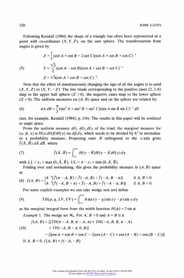
328 JOHN GATES

Following Kendall (1984) the shape of a triangle has often been represented as a point with co-ordinates (X, Y, Z), on the unit sphere. The transformation from angles is given by

1 Z = - (cot A + cot B - 2 cot C)(cot A + cot B + cot C)-' 2

(5) Y= -N (cot A - cot B)(cot A + cot B + cot C)- 2

Z = 3(cot A + cot B + cot C)-' Note that the effect of simultaneously changing the sign of all the angles is to send

(X, Y, Z) to (X, Y, -Z). The line triads corresponding to the positive cases (2, 3, 6) map to the upper half sphere (Z > 0), the negative cases map to the lower sphere (Z < 0). The uniform measures on (A, B) space and on the sphere are related by:

(6) dA dB = - (sin2 A + sin2 B + sin2 C)(sin A sin B sin C)-' dS 3

(see, for example, Kendall (1984), p. 116). The results in this paper will be confined to angle space.

From the uniform measure dG1 dG2 dG3 of the triad, the marginal measure for (a, 3, y) is H(a)H(P)H(y) da df dy, which needs to be divided by h3 to normalise to a probability measure. Projecting onto W orthogonal to the y-axis gives j(A, B) dA dB, where

UL

(7) (AB)= H(y - B)H(y - A)H(y) dy

with LL = e1 + max (0, A, B), UL = 7 - E2 + min (0, A, B). Folding over and normalising, this gives the probability measure in (A, B) space

as

(8) f(A,B)=

=h-3{f(r - A, B) +f(-A, B) +f(-A,

B - )}

if A, B >0 h-3{f(-A, B + z) +f(-A, B) +f(-A - ir, B)} if A, B <0.

For some explicit examples we can take wedge sets and define UV

(9) TH(p, q, LV, UV)=f 8sin(y - q)sin (y -p)sin ydy LV

as the marginal integral form from the width function H(0) = 2 sin ?.

Example 1. The wedge set Wo. For A, B > 0 and A + B - z,

f(A, B)= l{TH( - A, Br-A, ) + TH(-A, B, B, r - A)

(10) + TH(-A, B - r, O, B)}

= {cos A + cos B + cos C - ((cos (A - C) + cos (A - B) + cos (B - C))}.

If A, B <0, f(A, B) = f(-A, -B).




B

S- 2E 6

3,6 2,6

2 2,__\3,6 3 2,3 2

2E - 2E A

Figure 3. E < r/6

We consider further some of the wedge set cases. When E = 0 each shape can be achieved from three cases but when e > 0 some shapes can be achieved by some cases. For the positive cases, Case 2 requires A

_ 2E, Case 6 requires B ? 2E and

Case 3 requires C = 7- A - B 2E. Figure 3 shows which shapes can be obtained

by which cases. If E! r/6, all shapes can be achieved, but if E > 7r/6, the near-equilateral cases cannot; Figure 4 shows the situation for E = r/4, where only obtuse triangles can be realised.

Example 2. The wedge set W,/4. Suppose A is positive and the largest angle, then such triangles arise from Case 2 only.

f(A, B) = (2V2)-3TH(r - A, B, 5zr/4 - A, 3z/4)

(11) = 1 {3 cos B + 3 cos C - 2 cos (A - B) - 2 cos (A - C)

- sin (A - C) - sin (A - B)}.

If B is the largest angle (Case 6) or C is largest (Case 3), the obvious interchange is made in expression (11).

B Ir

6

r/2

3 2

A ir/2

ir

Figure 4. E = ir/4



330 JOHN GATES

4. Maximum angle and inter-line angle distributions

We shall now look at the magnitudes of the angles and so take A, B >0, A + B ? 7r. Angle A will be the maximum angle of the triangle if A B and 2A z r - B. Thus the distribution of the maximum angle M is given by the p.d.f.

g(m) = 6f f(m, B) dB if 7r/3 -5 m 5 7/2

(12) -2m

= 6 ff(m, B) dB if 7/2 - m _ r.

For Example 1, the wedge Wo, we find:

g(m) 3/4[(3m - r) cos m + 2 sin m - 2 sin 2m + sin 3m] ff/3 5 m

_ /2

gl(m) = 13/4[(7 - m) cos m + sin m - 2/3 sin 2m] z/2 m

For Example 2, the wedge W,/4, we find

g2(m) = [-2 sin 2m + cos 2m + sin m + cos m] z/2 5 m 5 z.

The maximum angle distributions for Example 1 and Example 2 are shown in Figure 5 and Figure 6.

For Example 1 we note that the terminal density g(7r) = 0, that is

Pr (max angle 7 -- 8) = o(8).

If g* denotes the maximum angle density for an arbitrary biset (L, R), then:

g*(m) 5 4ah(L, R)-'g,(m),

where a is chosen so that Wo(a) c (L, R). This inequality implies that g*(r) = 0 in

0.7 g(m)

0.6

0.5

0.4

0.3

0.2

0.1

1.5 2 2.5 3

Maximum angle, m

Figure 5. Example 1: E = 0




0.8 g(m)

0.4

0.2

1.75 2.25 2.5 2.75 3 Maximum angle, m

Figure 6. Example 2: E = 7r/4

general. Thus, for dual random triangles, the collinearity (or 'Broadbent') constant is zero unlike the case when a random triangle is defined by vertices (see Kendall and Kendall (1980) and Small (1982)).

We now consider the connection between the triangle shape distribution and the inter-line angle (ILA) distribution. If G' and G" are uniformly selected from (S(L, R) we can record the unsigned angle Q between them; Q has p.d.f. given by the covariance integral

(13) k(w) = 2h-2 H(O)H(o + w) dd.

In (13) the limits are somewhat nominal. For Example 1 the ILA p.d.f. is

(14) klI(w) = ?{sin w + (r - w) cos w} 0 r .

The ILA distribution can be thought of as the dual of the distribution of the distance IP1, - P21 between two points P1, P2 uniformly chosen in a convex set K.

Now the ILA distribution concerns the angle between two lines in (S(L, R) and the shape distribution concerns the angles between three such lines. It is almost immediate that the ILA distribution is marginal to the shape distribution, but this is not quite the case because whether w or n - w appears as the triangle angle depends upon the position of the third line. By either considering the distribution of min (Q, 7 - Q) or tracing vertical sections at w and 7r - w in the (A, B) domain back to vertical sections in the hexagon domain of Figure 2, we find:

(15) k(w) + k(7 - w) = 2{m, f(w) + m, f(l " -)},



332 JOHN GATES

where m, f is the marginal p.d.f. for one triangle angle,

1r-A

m lf

(A) ff(A, B) dB (for A > 0).

Suppose (L, R) has internal width function with support [E,, r - E2]; then if

o < El + E2, k(r - w) = 0 and (13) gives the ILA density in terms of mIf, which is derived from the shape distribution alone. In general we need the two terms on either side of (15). As an illustration we can check (15) for Example 1; we have, by integrating (10),

mf(A)= {sinA +( - A)cosA - 2/3 sin 2A} for 0-< A -

and k(w) given by (14). This confirms relationship (15) for Wo. The connection between the dual shape distribution and the ILA distribution has

no obvious analogue for connecting point-generated triangles and interpoint distances.

As another comment on features which have differing 'directness' in the dual versions, consider the ILA distribution as the dual of the interpoint distribution (or equivalently the chord length distribution) for a convex set K. The correlation theorem for the Fourier transform of (13) means that if R is the reflection of L both in the origin and the y-axis, then L and R can be determined from K by a direct process. On the other hand, the interpoint distribution for a convex set K contains a lot of information about K (but not always up to complete characterisation) but not in an explicit form. Similarly for three uniform points in K the triangle shape distribution contains much information about K (see Kendall and Le (1986)) but such in a way that reconstruction of K is not easy.

5. Further comment

The analysis in this paper has been for triangles constructed using three i.i.d. uniform lines. If we wished to generate triangles which were small perturbations of a parent triangle, we could take G,, G2, G3, uniform in separate convex line neighbourhoods, that is Gi a (~ (Li, Ri) for i = 1, 2, 3, where the ith parent triangle side passes between L, and Ri. If (Li, R,) has internal width function Hi, then the probability model starts with the marginal measure element f(A, B) dA dB, where

f (A, B) = f H(y - B)H2(y - A)H3(y) dy

and much of the preceding remains unchanged except for the details of Hi. On the other hand, if independence of lines is to be dropped we have a more




general interchange between triangles defined by points and triangles defined by lines. The appropriate connection was given by Blaschke as:

dP, dP2 dP3 = D03 dG1 dG2 dG3

(see Santal6 (1976), p. 59), D being the diameter of the circumcircle.

References

AMBARTZUMIAN, R. V. (1990) Factorization Calculus and Geometric Probability. Cambridge Univers-

ity Press. DRYDEN, I. L. AND MARDIA, K. V. (1991) General shape distributions in a plane. Adv. Appl. Prob.

23, 259-276. GATES, J. (1993) Some dual problems of geometric probability in the plane. Combinatorics,

Probability and Computing, 2, 11-23. KENDALL, D. G. (1984) Shape manifolds, procrustean metrics and complex projective space. Bull.

London Math. Soc. 16, 81-121. KENDALL, D. G. (1985) Exact distributions for shapes of random triangles in convex sets. Adv. Appl.

Prob. 17, 308-329.

KENDALL, D. G. AND KENDALL, W. S. (1980) Alignment in two-dimensional random sets of points. Adv. Appl. Prob. 12, 380-424.

KENDALL, D. G. AND LE, H.-L. (1986) Exact shape-densities for random triangles in convex polygons. In Analytic and Geometric Stochastics, Suppl. Adv. Prob., 59-72.

SANTAL6, L. A. (1976) Integral Geometry and Geometric Probability. Addison-Wesley, Reading, MA. SMALL, C. G. (1982) Random uniform triangles and the alignment problem. Math. Proc. Camb. Phil.

Soc. 91, 315-322.



shape distributions for planar triangles by dual construction

Documents