KTH ROYAL INSTITUTE OF TECHNOLOGY

SCHOOL OF ENGINEERING SCIENCES

DEPARTMENT OF LIGHTWEIGHT STRUCTURES

DEGREE PROJECT IN ENGINEERING PHYSICS,

SECOND CYCLE, 30 CREDITS

STOCKHOLM, SWEDEN 2016

Shape Distortion Analysis of

Self-Reinforced Poly(ethylene

terephthalate) Composites

The PETrifying reality!

CALLE ELIASSON

I

Acknowledgement The work presented in this thesis was performed as part of collaboration between Scania in

Södertälje and the Department of Lightweight Structures at KTH Royal Institute of

Technology in Stockholm. I would like to start off by thanking my four supervisors Lars

Jerpdal, Stefan Bruder, Malin Åkermo and Daniel Ståhlberg for all their support and guidance

throughout the whole project. I would also want to express my gratitude to everybody at the

UTMR department at Scania for turning this project into an enjoyable experience.

Last but not least a special thanks needs to be awarded to some honourable mentions: Bertil

Tamm and Claes Carlsson for their help with CATIA, Monica Norrby and Anders Beckman

for their painstaking work of trying to keeping the laboratory at the Department of

Lightweight Structures up and running and Roger Björk for his backbreaking work of

performing the entire 3D laser scanning of all the components.

II

Abstract Composite components with a V-shaped geometry have been manufactured through

compression moulding of fabrics based on self-reinforced poly(ethylene terephthalate). The

fabrics were subjected to a set of predetermined degrees of stretching during manufacturing

with the intent to investigate its effects on shape distortions in terms of spring-in and warping.

The shape distortions were also monitored as the components were subjected to sawing, a

secondary heat treatment and a secondary chemical treatment. Moreover, to a limited extent

the effects of weave architecture and pattern orientation were also studied as both twill and

plain weaves used and the fabrics were rotated a relative angle of 45°. The shape distortions in

these were then compared with shape distortions in both un-stretched self-reinforced

poly(ethylene terephthalate) and traditional composite components based on

glass/poly(ethylene terephthalate) and carbon/poly(ethylene terephthalate). Laser scanning

measurements of the surfaces showed that fibre stretching counteracted spring-in while

causing warping in the components during manufacturing. Sawing had limited effects on the

components while heating increased spring-in but reduced warping. The chemical treatment

increased both the spring-in and warping to a smaller and larger extent than the heat treatment,

respectively. Overall the carbon fibre components performed best but the self-reinforced

poly(ethylene terephthalate) performed better than the glass fibre ones. Lastly, both the

secondary processing steps had a negative effect on the surface quality.

III

Sammanfattning V-formade kompositartiklar har tillverkats genom formpressning av vävar bestående av

självförstärkt polyetentereftalat. Under tillverkningsfasen utsattes materialet för

förutbestämda sträcknings grader samt tilläts förblev osträckt med för avsikt att kartlägga

fibersträckningen påverkan på formförändringar så som spring-in och skevning. Effekterna av

sågning, värme- och kemikalieytbehandling på uppkomsten av formförändringar

inspekterades. Utöver detta undersöktes även effekten av vävstruktur (tuskaft och twill

testades) samt orientering av dessa, då de utsattes för en relativ rotation på 45 ° , i viss

omfattning. Dessutom utfördes en jämförelse mellan de inducerade formförändringarna i de

självförstärkta polyetentereftalat komponenterna och mer traditionella kompositkomponenter

baserade på glasfiber/polyetentereftalat samt kolfiber/polyetentereftalat för fallet med osträckt

material. De erhållna resultaten påvisar att fibersträckning minskade spring-in-vinkeln i

komponenteran efter tillverkning medan skevning istället uppstod. Sågning hade en begränsad

effekt på formförändringarna. Värmebehandlingen hade större påverkan på komponenterna

och resulterade i en ökande spring-in-vinkel men dock en minskad skevning. Kemikaliernas

påverkan på spring-in-vinkeln var relativt liten i relation till värmebehandlingen medan

påverkan på skevningen var mer påtaglig. Överlag presterade kolfiberkomponenterna bäst

emellertid klarade sig de självförstärkta komponenterna i regel bättre än

glasfiberkomponenterna. Båda efterbehandlingsprocesserna påverkade texturen på

komponentera som blev märkbart grövre och strävare.

IV

Abbreviations and nomenclature

Abbreviations Nomenclature

C Chemical Treated 𝑇𝑔 Glass Transition Temperature

CFRC Carbon Fibre Reinforced Carbon 𝑇𝑐 Crystallisation Temperature

CMC Ceramic-Matrix Composite 𝑇𝑚 Melting Temperature

CTE Coefficient of Thermal Expansion 𝑥𝑓𝑙𝑜𝑤 Flow Distance of Matrix

EP Epoxy 𝑡𝑓𝑙𝑜𝑤 Duration of Matrix Flow

FRC Fibre Reinforced Composite 𝑝𝑎𝑝𝑝𝑙𝑖𝑒𝑑 Applied Pressure During Flow

FRP Fibre Reinforced Plastic 𝑛𝑜𝑣𝑒𝑟 Number of Passed Over Tows

H Heat Treated 𝑛𝑢𝑛𝑑𝑒𝑟 Number of Passed Under Tows

HTPET High Tenacity PET 𝑑 Length of Baseline

LPET Low melting point PET

𝑥1 Distance Between Laser and

Target

M Manufactured

𝑥2 Distance Between Camera and

Target

MMC Metal-Matrix Composite 𝜃 Angle

P Plain Weave Architecture 𝜙 Spring-in Angle

PC Polymer Composite 𝑖 Index

PE Polyethylene 𝒗 Vector

PEEK Poly(Ether Ether Ketone) 𝒖 Vector

PET Poly(Ethylene Terephthalate) 𝑃1 Set of process parameters

PP Polypropylene 𝑃2 Set of process parameters

PUR Polyurethane

RTM Resin Transfer Moulding

S Sawed and Untreated

SrC Self-reinforced Composite

SrPC Self-reinforced Polymer

Composite

SrPET Self-reinforced PET

STF Stress Free Temperature

T Twill Weave Architecture

UD Unidirectional

UP Unsaturated Polyester

VE Vinyl Ester

V

Table of contents

Acknowledgement ....................................................................................................................... I

Abstract ..................................................................................................................................... II

Sammanfattning ....................................................................................................................... III

Abbreviations and nomenclature .............................................................................................. IV

Table of contents ....................................................................................................................... V

1 Introduction ......................................................................................................................... 1

2 Theory ................................................................................................................................. 3

2.1 Composites .................................................................................................................. 3

2.1.1 Fibres .................................................................................................................... 4

2.1.2 Matrices ................................................................................................................ 4

2.2 Polymers ...................................................................................................................... 5

2.2.1 Thermoplastics ..................................................................................................... 5

2.2.2 Thermosets ........................................................................................................... 9

2.3 Self-reinforced composites .......................................................................................... 9

2.4 Manufacturing ........................................................................................................... 10

2.4.1 Commingling ...................................................................................................... 11

2.4.2 Woven fabrics .................................................................................................... 12

2.4.3 Compression moulding ...................................................................................... 13

2.4.4 Manufacturing of self-reinforced polymer composites ...................................... 14

2.5 Shape distortion ......................................................................................................... 16

2.5.1 Thermal properties of the constituents ............................................................... 17

2.5.2 Shrinkage ............................................................................................................ 18

2.5.3 Stress free temperature ....................................................................................... 19

2.5.4 Through-thickness variations ............................................................................. 19

2.5.5 Stretching of fibres ............................................................................................. 20

2.6 Measurement techniques ........................................................................................... 20

2.6.1 Triangulation ...................................................................................................... 20

2.6.2 3D laser scanning ............................................................................................... 21

3 Materials ........................................................................................................................... 21

4 Method .............................................................................................................................. 22

4.1 Manufacturing of test specimens ............................................................................... 22

4.2 Secondary processing ................................................................................................ 26

4.2.1 Heat treatment .................................................................................................... 27

VI

4.2.2 Chemical treatment ............................................................................................ 27

4.3 Measurements of shape distortions ............................................................................ 27

5 Results ............................................................................................................................... 31

5.1.1 Quality of the manufactured components .......................................................... 31

5.1.2 Measured shape distortions ................................................................................ 33

6 Discussion ......................................................................................................................... 37

6.1 Discussion of results .................................................................................................. 37

6.1.1 M components .................................................................................................... 37

6.1.2 S components ..................................................................................................... 38

6.1.3 H components ..................................................................................................... 38

6.1.4 C components ..................................................................................................... 39

6.1.5 Surface quality .................................................................................................... 39

6.2 Sources of error ......................................................................................................... 39

6.2.1 Overheating of the material ................................................................................ 40

6.2.2 Misalignment of the tool halves during closure ................................................. 40

6.2.3 Thickness difference between the two symmetry halves of the cross section ... 41

6.2.4 Slippage in the clamping devices ....................................................................... 42

6.2.5 Indentations in the component surfaces ............................................................. 42

6.2.6 2D stretching of the twill material ...................................................................... 43

6.2.7 Lack of reference points on the components ...................................................... 44

6.2.8 Resolution of the laser scanner ........................................................................... 44

6.2.9 Transparency of the LPET matrix ...................................................................... 44

7 Conclusions ....................................................................................................................... 44

References ................................................................................................................................ 46

1

1 Introduction At the dawn of man, mankind quickly realised the importance of tools and equipment to

facilitate everyday tasks of survival. A common belief is that these very instruments have

been one of the major driving forces in the evolution of us humans. Materials have thus

implicitly played a key role throughout history and have left a considerable mark as a new

material has been discovered or tamed. The Stone Age, Bronze Age and Iron Age are three

famous eras which were governed by immense technological advancements defined by new

knowledge about a material. It is therefore not unnatural to assume that the hunt for new and

improved materials have incused today’s science. Composite materials have been around for a

long time, even as far back as around 3400 B.C. as the Mesopotamian people created plywood

by adhesively joining strips of wood at different angles. [1] However, it was not until the

twentieth century that the term “composite materials” became synonym with the engineering

plastics that they associated with today.

In the year of 1931 the company Owens Illinois Glass Company introduced to the world the

first commercially feasible production method of glass fibres. At the time the main usage of

glass fibres was as thermal insulation used during construction of houses. Still, the availability

of glass fibres acted as a starting point for the modern field of composites. Four years later

Owens Illinois Glass Company formed a partnership with Corning Glass Works, and later

merged into Owens Corning in 1938, during which they launched the world’s first fibre

reinforced polymer composite. The following years several new plastics were invented, for

example, the unsaturated polyester (1936) and epoxies (1938) allowing the already growing

composite industry to further gain momentum. Development continued and several new

manufacturing methods for composites emerged together with new types of fibres, for

example, the strong carbon fibres which opened up a new world of high performance

composites. [1] [2]

One of the classical problems of composite manufacturing is to ensure that the bonds between

the constituents are of high quality. N. Capiati and R. Porter studied this problem during the

70’s and realised that the bond quality could be enhanced by minimising the chemical

difference between the constituents. They therefore introduced the idea to use only one

constituent for all the different components in the composite which they reported in one of

their articles published in 1975. [3] In their work they manufactured polymer composites

based entirely on polyethylene, consisting of polyethylene filaments embedded in a similar

type of polyethylene chosen as to maximise the molecular weight difference between the two

types. This together with the thermodynamically more stable crystals in the filaments resulted

in a large enough difference in melting point to allow for the composite to be manufactured.

They then tested the bond quality by performing shear pull-out tests in which the stresses

needed to break the bonds were recorded from the outer surface of the filaments. The values

they acquired fell in-between the characteristic values of glass fibre reinforced polyester and

glass fibre reinforced epoxy. However, they concluded that the bonds in the polyethylene

composite consisted of epitaxy bonds to a higher degree rather than the compressive type

caused by the shrinkage in the polyester and epoxy, respectively, in the reference materials.

This means that the crystal structures in the two polyethylene constituents have grown into

each other forming a merged structure.

Their pioneering work paved the way for a new branch of the composite industry dealing with

the new so called “self-reinforced” materials, especially the polymeric types due to the

2

recyclability aspect. Several studies have been conducted to improve and further develop the

original idea of N. Capiati and R. Porter.

One of these is a study published in 1978 by W. Mead and R. Porter. [4] They investigated the

possibility of creating self-reinforced polyethylene composites by stacking layers of highly

oriented strips and films on top of each other. The stack is then heated and the films melt and

flow around the strips. This method is to day referred to as bi-component film stacking.

Among other things they also varied the in-plane orientation of the reinforcing strips and the

volume fraction of these in the material while measuring its elastic modulus. W. Mead and R.

Porter reported that the method was successful and that the measured elastic moduli were in

good agreement with predictions based on the rule of mixtures.

T. Peijs published an article in 2003 in which he presented another way of manufacturing self-

reinforced polymer composites termed PURE. The method is based on a tape laying

technology in which layers of additional plastic, with a low melting point, is applied to the

reinforcing tapes. When heat and pressure is applied this extra layer melts and embeds the

reinforcement, creating a composite structure. Tapes were chosen rather than fibres, with their

round cross sections, due to the possibility of increased degree of packing. [5]

L. Jerpdal and M. Åkermo have studied the influence of fibre stretching and shrinkage, which

occur during manufacturing, on both tensile and compressive properties as well as crimp in an

article published in 2014. [6] This was performed using laminates of self-reinforced

poly(ethylene terephthalate) manufacturing using compression moulding of plain weaves

which were allowed to shrink or be subjected to different degrees of stretching. They reported

in terms of crimp the introduced shrinkage had a much larger impact than the stretching.

However, the opposite behaviour was observed regarding the mechanical properties as the

shrinkage had a minute impact in relation to the additional fibre stretching. It was for example

shown that a fibre stretching of 10% resulted in an increase in tensile modulus of 50%. L.

Jerpdal and M. Åkermo therefore concluded that for the laminates in question the mechanical

properties were dominated by the microstructure of the material rather than the

macrostructure.

C. Schneider et al. studied the possibility of creating a sandwich structure made entirely from

self-reinforced poly(ethylene terephthalate) in an article published in 2015. [7] They came up

with a concept of a corrugated sandwich panel consisting of two face sheets resting on a core

made up of a set of closely packed hollow isosceles trapezoidal beams. The wall thickness to

height of the cross section ratio of the trapezoids were varied and while the dynamic

compressive response of the panels were evaluated for different stain rates. C. Schneider et al.

reported that rate had a minor effect on the strength and stiffness of regular laminates similar

to the face sheets. However, an increasing strain rate resulted in a substantially enhancement

of the yield strength. In terms of the sandwich panels the structures with cores consisting of

beams with a slender cross section also showed a large strength enhancement with a more

rapid loading. The opposite was observed for structures with a stubby cross section.

The aim of the present study is to investigate the formation of shape distortions, in terms of

angular changes, in self-reinforced polymer composites related to both manufacturing and to

some extent also secondary processing For this V-shaped components will be manufactured

thought compression moulding of commingled weaves based on poly(ethylene terephthalate).

The main focus will be to determine the impact of fibre stretching but several other aspects

will be studied as well. Two types of weave architectures will be tested (plain and twill) and

the orientation of the main fibres will be varied. A comparison between the performance of

3

the self-reinforced composites and traditional carbon- and glass reinforced versions of the

used matrix will also be included.

2 Theory In the following sections below the theory that will be needed will thought out the present

paper is outlined. To begin with the concepts of composite materials, fibres and matrices are

presented along with a section on polymers, which play a key role in today’s composite

industry. Thereafter, the special case of self-reinforced composites is introduced followed by

two sections focusing on some of the aspects of manufacturing and measurement techniques,

respectively. Lastly, the mechanics of shape distortion with an emphasis on fibre reinforce

thermoplastics are discussed in a section that concludes the theory section as a whole.

2.1 Composites The term “composite” refers to a material system which is comprised out of a minimum of

two different materials that have been mixed together on a macroscopic scale. The idea is to

try and create a combination in which the negative properties of the constituents have been

suppressed and new positive properties have been gained. There are several different types of

composite materials both naturally occurring materials, such as wood, and manmade, such as

reinforced glass.

Figure 2.1: Four common ways of distributing the fibrous reinforcements in a laminate or ply.

Composite materials are becoming increasingly more popular in engineering, especially the

class called fibre reinforced composites (FRC) due to their high stiffness to mass and strength

to mass ratios. The FRCs may have either long (continuous) or short (discontinuous) fibres

which can be oriented or randomly arranged, see Figure 2.1. In applications demanding high

performance, composites with oriented continuous fibres are predominant. These FRCs

consist of thin sheets, called plies, which are considered orthotropic. The plies are typically

unidirectional (UD) fibres imbedded in a matrix characterised by a local coordinate system

with its principal axis (called the 1-direction) pointing along the fibres. These plies are then

rotated some angle relative to a global axis and stacked together to form a laminate, also

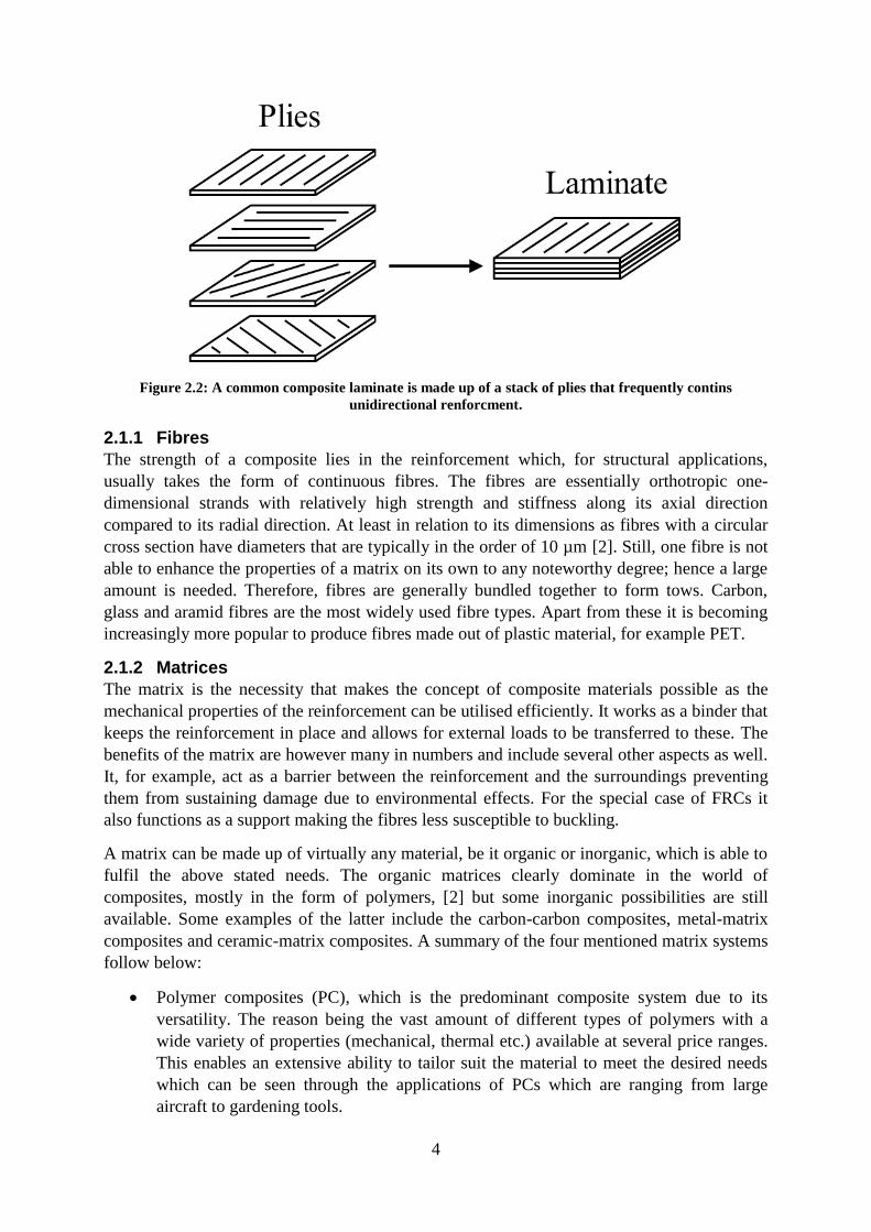
considered orthotropic, see Figure 2.2.

4

Figure 2.2: A common composite laminate is made up of a stack of plies that frequently contins

unidirectional renforcment.

2.1.1 Fibres

The strength of a composite lies in the reinforcement which, for structural applications,

usually takes the form of continuous fibres. The fibres are essentially orthotropic one-

dimensional strands with relatively high strength and stiffness along its axial direction

compared to its radial direction. At least in relation to its dimensions as fibres with a circular

cross section have diameters that are typically in the order of 10 µm [2]. Still, one fibre is not

able to enhance the properties of a matrix on its own to any noteworthy degree; hence a large

amount is needed. Therefore, fibres are generally bundled together to form tows. Carbon,

glass and aramid fibres are the most widely used fibre types. Apart from these it is becoming

increasingly more popular to produce fibres made out of plastic material, for example PET.

2.1.2 Matrices

The matrix is the necessity that makes the concept of composite materials possible as the

mechanical properties of the reinforcement can be utilised efficiently. It works as a binder that

keeps the reinforcement in place and allows for external loads to be transferred to these. The

benefits of the matrix are however many in numbers and include several other aspects as well.

It, for example, act as a barrier between the reinforcement and the surroundings preventing

them from sustaining damage due to environmental effects. For the special case of FRCs it

also functions as a support making the fibres less susceptible to buckling.

A matrix can be made up of virtually any material, be it organic or inorganic, which is able to

fulfil the above stated needs. The organic matrices clearly dominate in the world of

composites, mostly in the form of polymers, [2] but some inorganic possibilities are still

available. Some examples of the latter include the carbon-carbon composites, metal-matrix

composites and ceramic-matrix composites. A summary of the four mentioned matrix systems

follow below:

Polymer composites (PC), which is the predominant composite system due to its

versatility. The reason being the vast amount of different types of polymers with a

wide variety of properties (mechanical, thermal etc.) available at several price ranges.

This enables an extensive ability to tailor suit the material to meet the desired needs

which can be seen through the applications of PCs which are ranging from large

aircraft to gardening tools.

5

Carbon-carbon composites or carbon fibre reinforced carbon (CFRC), which is an

extremely costly class of materials with low density and high end mechanical

properties that remain unaltered for service temperatures reaching above 2000 °C .

These materials are usually found in heat shield applications (e.g. for space shuttles)

but also in brake disks for race cars. [2]

Metal-matrix composites (MMC), having high densities, good properties, and better

thermal resistance than polymeric matrices. Applications where MMCs are usually

found are satellites and engines for both rockets and jet aircraft. [2]

Ceramic-matrix composites (CMC), with both high mechanical as well as thermal

properties. The reinforcements are added with the hopes of making the ceramics less

brittle and follow a more predictable behaviour during failure. The common

applications of CMCs are similar to those of both CFRCs and MMCs, namely heat

shields and propulsion systems. [2]

2.2 Polymers Polymers are long molecules consisting of a large number of smaller units called monomers.

The monomers are bonded together in a chain-like configuration by means of strong primary

bonds and can form different types of architectures such as linear, branched and networked.

These bonds in-between monomers are known as intramolecular bonds. Apart from these

possible architectures, which are related to the structure of the molecular chains themselves,

the arrangement of the molecules relative to each other is of importance as well. This involves

how the bonds in-between molecules (intermolecular bonds) act and the global formation of

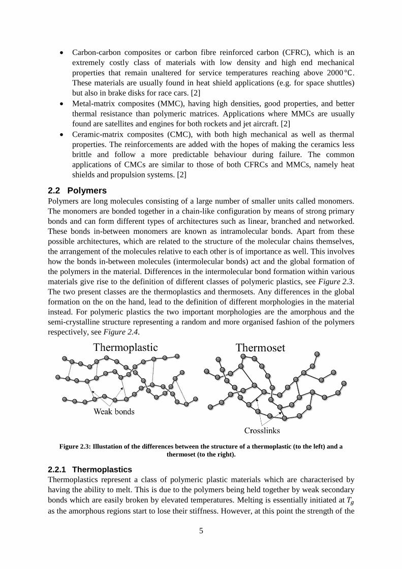
the polymers in the material. Differences in the intermolecular bond formation within various

materials give rise to the definition of different classes of polymeric plastics, see Figure 2.3.

The two present classes are the thermoplastics and thermosets. Any differences in the global

formation on the on the hand, lead to the definition of different morphologies in the material

instead. For polymeric plastics the two important morphologies are the amorphous and the

semi-crystalline structure representing a random and more organised fashion of the polymers

respectively, see Figure 2.4.

Figure 2.3: Illustation of the differences between the structure of a thermoplastic (to the left) and a

thermoset (to the right).

2.2.1 Thermoplastics

Thermoplastics represent a class of polymeric plastic materials which are characterised by

having the ability to melt. This is due to the polymers being held together by weak secondary

bonds which are easily broken by elevated temperatures. Melting is essentially initiated at 𝑇𝑔

as the amorphous regions start to lose their stiffness. However, at this point the strength of the

6

crystallites is still preserved meaning that semi-crystalline thermoplastics are still structurally

stable at 𝑇𝑔. It is not until the melting temperature 𝑇𝑚 is reached before the crystallites start to

dissolve and the material melts completely. [8] The melting aspect opens up the possibility of

recyclability which is considered to be one of the main befits of thermoplastic matrices.

The weakness of the intermolecular bonds also affects the mechanical properties of the

thermoplastics which are generally considered rather poor. However, as they are mostly

ductile they are tough and durable.

Figure 2.4: Visualisations of an amorphously oriented polymer molecule (to the left) and a more

structured semi-crystalline (to the right).

As the molecules are relatively loosely bound to each other they can arrange in different

ways, making it possible to form both amorphous and crystalline structures. Thermoplastics

can thus be either amorphous or semi-crystalline, see Figure 2.4 and 2.2.1.1 Crystallisation.

The crystalline regions make the material stronger, more temperature tolerant and less

susceptible to sustaining damage from solvents than the amorphous. However, the

thermoplastic becomes more brittle the higher the crystalline content which need to be taken

into account depending on the application.

Some examples of thermoplastics are polyethylene (PE), polypropylene (PP), poly(ethylene

terephthalate) (PET) and poly(ether ether ketone) (PEEK).

2.2.1.1 Crystallisation

In the world of polymer science, crystallisation is a process in which a polymer arranges parts

of its molecular chains in regularly distributed lumps called crystals. These crystals are made

up of molecules folded in a “zigzag” like pattern where one molecule can be part of several

crystallites. These formations are plane in structure and can be stacked on top of each other in

an out-of-plane fashion creating lamellar crystals, see Figure 2.5. The crystallite structure is

very beneficial as is corresponds a state of minimum energy implying that the creation of

crystals, the crystallisation process, is exothermal. A way of characterising the amount and

extent of the crystallite regions is done through the concept of degree of crystallinity which is

always below 100%. This is due to the polymer molecules having non-uniform molar mass

and that the crystallisation time would be tremendously long in order to reach the ideal state

of 100% crystallinity. [9] Polymers having the intrinsic property of forming crystallites are

7

thus referred to as semi-crystalline as there will be amorphous regions present to some extent

as well. Crystallisation is highly dependent on the cooling rate of the material since the

process is fairly slow. A too rapid cooldown below 𝑇𝑔 will lock the current structure in place.

There also exists an optimal span of temperatures for which crystals are formed. [2] The most

ideal temperature in this range is called the crystallisation temperature, 𝑇𝑐.

Figure 2.5: Depiction of lamellar crystal structures and the amorphous regions connecting them. Redrawn

from reference. [2]

Apart from this natural crystallisation there can also exist what is referred to as deformation-

induced crystallisation. Deformation-induced crystallisation is the establishment of crystals, in

the form of parallel molecules, which arise due to deformations such as stretching or shearing.

As a result of the deformation the long polymer chains are forced to run parallel to the applied

shear forces or the direction of elongation. This principle is the basis for creation of polymeric

fibres, see 2.2.1.3 PET fibres. This imposed orientation increases the free energy in the

material [10] which may be released at a later instance, for example during unloading or

heating. The order of the molecules is then beginning to revert back towards the original

structure. Therefore the fibres need to be quenched in order to allow for the new orientation to

be kept and to render the fibres structurally stable.

2.2.1.2 PET

For a structural engineer the name “polyester” usually steer ones thoughts towards

thermosetting plastics, especially the predominant unsaturated polyester (UP) which is

widespread within the composite industry. However, polyesters also have thermoplastic

counterparts, simply referred to as “thermoplastic polyesters”. One example of these is

poly(ethylene terephthalate) (PET) which is a semi-crystalline plastic capable of forming a

degree of crystallinity up to 30-40% [11] but also as low as 0%, i.e. being completely

amorphous. However, the maximum possible degree of crystallinity is dependent on a wide

range of parameters; hence this limit may vary between different types of PET.

The glass transition temperature of PET is roughly 𝑇𝑔 = 80°C while the melting temperature is

in the neighbourhood of 260°C < 𝑇𝑚 < 265°C.

8

It is rather common to stumble upon not only standard PET but also modified versions of PET,

be it of chemical or post-processing nature. [12] The aim is, of course, to generate a final

product having some specific features in relation to the starting material. One example that is

not so widely used in industry to date is the low melting point poly(ethylene terephthalate)

(LPET) while the high tenacity poly(ethylene terephthalate) (HTPET) is used more

extensively.

LPET is a chemically modified version of standard PET where the main focus has

been to substantially lower the melting point. The material becomes a liquid at

approximately 160-180°C.

HTPET is based on standard PET but has an increased Young’s modulus. It comes in

the form of fibres and the increase in the elastic modulus has been induced by drawing

in the fibre manufacturing process, see 2.2.1.3 PET fibres. It should thus not be

regarded as a new distinct material but rather as an alternative form of the standard

PET itself.

Even though the industrial applications are few in numbers for LPET, the combination of

LPET and HTPET enables the creation and processing of composite materials based on only

one constituent, see 2.3 Self-reinforced composites. This type of material system is very

interesting from a research point of view.

When it comes to manufacturing and processing of PET it should be noted that it is very

sensitive to hydrolysis. Due to the microstructure of PET, water diffuses into the amorphous

regions of the polymer when it is heated above 𝑇𝑔 in wet or humid conditions or if there is

already moisture present in the material. The water then starts to degrade the material by

means of chain scission in which the length of the polymers is reduced. Therefore, PET

should be dried for some time prior to processing to avoid any unnecessary lowering of the

quality of the material. [13] [14]

2.2.1.3 PET fibres

Among the most widespread synthetic fibres in use today are those based on PET and can be

found in a wide range of different applications. The success of PET fibres lies in their good

mechanical properties in relation to the low-cost raw material and production methods

available. [12]

The most predominant manufacturing method for the production of PET fibres is the melt

spinning process. A liquid of molten polymer is fed to a chamber containing holes through

which the melt is extruded to form fibrous structures. This step orients the polymer molecules

so that the strong primary bonds are directed along the axial direction. [2] The material

becomes strengthened along the longitudinal direction of the extruded structure as a state of

higher crystallinity is achieved. However, at this stage the mechanical properties of the

polymer strands are still rather poor as the degree of crystallinity is relatively low. In an

attempt to improve upon these, the fibres are stretched in a drawing process which further

increases the degree of orientation of the molecules. Before the drawing procedure can

commence though, the fibres have to become more structurally stable so that the newly

extruded shape is kept. The fibres are thus let to solidify and cool down below 𝑇𝑚 by the use

of a stream of cold air. Furthermore, by keeping the fibres above 𝑇𝑔 the deformation due to

the stretching is uniformly distributed along the total length. For temperatures below 𝑇𝑔 the

9

fibres have a tendency to experience the phenomena of necking which may lead to localised

failure. [15]

The extrusion speed is very important in determining the properties of the fibres as the

magnitude of the shear forces, acting on the fibre walls from the extrusion holes, is influenced

by this. This in turn determine the degree of deformation-induced crystallisation and hence

the mechanical properties. For a low extrusion speed the shear forces are also low, and will

thus result in low degree of orientation. The opposite can be said for high extrusion speeds. A

too high pulling speed is not desirable however, as it may cause the fibres to rapture. [12]

Regarding the raw material it is unwanted to have a plastic which already have a significant

amount of crystalline formations. These contribute to the overall strength and stiffness of the

material and a too stiff material may break during manufacturing. [12]

2.2.2 Thermosets

The thermoset class of polymeric plastics is to some extent the opposite of that of

thermoplastics. The intermolecular bonds are comprised out of primary bond which are

formed in a process called crosslinking, involving exothermal chemical reactions. Thus, the

bonds in-between molecules are of the same type as those holding adjacent monomers in

place, rendering it ambiguous to talk about different individual polymers chains in a

crosslinked thermoset. To a certain extent a thermoset is comprised of only one, although,

colossal three-dimensional molecule! This implies that the thermosets lack the ability to melt

as the intermolecular bonds are broken at the same time as the intramolecular bonds (i.e. the

same instance as the polymer structures are broken down). Instead the thermoset reduces to a

lump of charred material making it harder to recycle. Moreover, the crosslinking process is

irreversible further reducing the ability to recycle the material.

As the primary bonds are an order of magnitude stronger than the secondary bonds [2] the

thermosets generally may achieve better mechanical as well as thermal properties than

thermoplastics. However, the brittleness is also increased making them less durable and

resistant to continuous wear and tear.

Due to the nature of crosslinking (the intermolecular bonds are formed in-between molecule

in a random manner forming one large molecule), the morphology of a thermoset always ends

up amorphous. The thermosets thus generally have less resistance towards solvents compared

to thermoplastics. [2]

Some examples of thermosets are unsaturated polyester (UP), vinyl ester (VE), polyurethane

(PUR) and epoxy (EP).

2.3 Self-reinforced composites Self-reinforced composite (SrC) is one of the many names referring to a special class of

composite materials in which both the reinforcement and matrix are of the same material.

Polymers are usually the foundation for these and are then instead referred to as self-

reinforced polymer composites (SrPC). Even though SrPCs share the same conceptual idea of

having a reinforced matrix, just as a traditional composite, the very definition of a composite

is challenged. Strictly speaking, as only one material is used for both the reinforcement and

matrix the minimum requirement of at least two materials is not fulfilled. Nevertheless, SrPC

are still of great interest in today’s research of composite materials.

10

The reinforcement and matrix are generally of different chemical nature, thus implying that

the quality of the bond between these is compromised. The concept of SrPC was therefore

introduced in 1975 by N. Capiati and R. Porter. [3] They realised that having the same

material throughout the composite would ensure better conditions for the formation of bonds.

Apart from the benefit of having strong bonds, SrPCs are easily and fully recyclable since the

whole material can be melted without the need to extract any fibres. This is one of the main

reasons why the SrPC concept is of high interest. Another perspective of the recyclability

aspect is instead that the self-reinforced polymer composites have rather low thermal

resistance. At elevate temperatures the fibres lose their deformation-induced crystallinity and

become indistinguishable from the surrounding matrix. [16]

Even though the mechanical properties of the polymer fibres are enhanced several times

during manufacturing compared to the matrix, the mechanical properties of these are still

relatively poor. However, for a SrPC it is possible to achieve a much higher fibre volume

fraction, as much as 90% [16] [17], compared to a traditional composite, for which 70% is a

more reasonable maximum level [2]. If these contributions to the mechanical properties are

considered together with the possibility of stronger bonds, the resultant material may have

decent properties. In some cases SrPC materials may even compete with certain types of glass

reinforces polymer composites. [17]

A high fibre volume fraction usually implies an increase in the overall mass of the material,

but not for a SrPC as the reinforcement and matrix have comparable densities. They are thus

very weight effective.

Lastly, SrPCs might be less cost effective to manufacture in contrast to conventional

composites. The reason being the more precise processing parameters needed, due to the more

narrow range of these, together with the exclusive manufacturing techniques. Moreover,

thermoplastics are generally rather sensitive to being exposed to elevated temperatures,

rendering the polymeric fibres even more susceptible to degradation than traditional ones. [16]

2.4 Manufacturing Manufacturing of composite structures requires new ways of thinking as new aspects are

introduced in the design process utilised in today’s industry. Apart from the unusual

anisotropic behaviour of the material systems themselves the choice of manufacturing process

as well as process related parameters play a much greater role than usual. One of the notable

changes is that composite materials are seldom created in a sub step of the manufacturing, and

in other words rarely used as raw material in itself. Instead, the raw material and the finished

product are made simultaneously in the same process, but there are of course some exceptions.

Pre-impregnated material (prepregs) can be used during manufacturing which would then

represent the use of a raw material. Needless to say, the production of composites components

is generally of a complex nature and the need for more specialised method is evident.

There is a vast array of available manufacturing methods to choose from when composite

components are produced; all of which are suited for a set of specific situations. The

complexity of the component geometry, the type of reinforcement and matrix, cost

effectiveness and time efficiency are all examples of parameters having a substantial impact

on which of these are appropriate. Commonly there are also two different versions of each

manufacturing process: one suited for thermoplastics and one for thermosets. The reason

being that they are of such different chemical nature. A thermoset generally have rather low

viscosity and cures through exothermal chemical reaction producing a great deal of excess

11

heat. The fluid-like behaviour of the uncured resin makes it beneficial to rely on techniques

involving a lot of flow such as spraying or suction. Due to the slow nature of the crosslinking

the manufacturing times tend to be long. On the contrary, thermoplastics are normally very

viscous, even in their molten form, which calls for a slightly different processing approach. A

substantial amount of flow is not achievable. Instead, prepregs and moulding compounds, see

2.4.3 Compression moulding, are formed to the desired shape using heat and mechanical

pressure. Since thermoplastic “setting” does not involve any chemical reactions the

manufacturing times tend to be much lower than for thermosetting components.

Some examples of frequently occurring methods in today’s industry are, RTM (Resin

Transfer Moulding), vacuum injection moulding, compression moulding and pultrusion.

2.4.1 Commingling

The wetting phase of the manufacturing, in which the fibres are impregnated, is of large

significance. In order to utilise the superior mechanical properties of the fibres, high quality

bonds between these and the matrix need to be ensured. If the fibres are not impregnated, and

thus lack contact with the matrix, load transfer simply cannot occur. A great deal of effort is

therefore put into trying to improve this stage. A common approach is to pre-impregnate the

reinforcement prior to the manufacturing of the component in question, which can be realised

with different procedures. Among the available methods are: solvent impregnation, melt

impregnation, powder impregnation and commingling. [2]

Commingled reinforcement is a mixture of thermoplastic matrix fibres and reinforcing fibres

that are brought together (commingled) to form UD tows which in turn may be used to form

fabrics. The idea is to bring the matrix closer to the reinforcement reducing the flow distance,

see Figure 2.6. Since, according to Darcy’s law:

𝑡𝑓𝑙𝑜𝑤 ∝𝑥𝑓𝑙𝑜𝑤

2

𝑝𝑎𝑝𝑝𝑙𝑖𝑒𝑑 (1)

where 𝑡𝑓𝑙𝑜𝑤 is the flow time, 𝑥𝑓𝑙𝑜𝑤 the flow distance and 𝑝𝑎𝑝𝑝𝑙𝑖𝑒𝑑 the applied pressure. In

other words, the time it takes for the matrix to flow a certain distance is proportional to the

square of the flow distance and inversely proportional to the applied pressure. [18]

Furthermore, as the matrix is already distributed in-between the fibres in the tows the

resulting wetting is more uniform and a greater share of the fibres are embedded.

Figure 2.6: The concept of commingling. The reinforcing fibres are brought together with the matrix

fibres to form a hybrid yarn. Redrawn from reference. [18]

12

The matrix material is mostly a modified version of the reinforcement polymer as to make the

melting temperature 𝑇𝑚 lower. By reducing this, a lower processing temperature is of course

required during manufacturing, hence the risk of thermal degradation and loss of orientation

in the fibres is reduced.

2.4.2 Woven fabrics

As mentioned above in 2.1.1 Fibres, it is a common practise to bundle individual fibres

together to form tows to facilitate the handling of the reinforcement. These tows can then be

further assembled into fabrics by grouping several tows together by, for example, means of

braiding, weaving and knitting.

Weaving is a way to merge 0° tows (termed warps) and 90° (termed wefts) into a sort of

chessboard like structure. The structure is created by the interlacing of the warps and wefts

such that they pass over and under each other in an ordered fashion. The fibres are thus not

completely straight but rather sinusoidal as they run along the fabric. To characterise the

textiles the degree of waviness of the fibres is measured in terms of crimp. Crimp indicates

how long the fibres are in relation to the length of the fabric. Depending on the situation

crimp can be both good and bad, for example, a high level of crimp allows for tight weaves at

the cost of lowered mechanical properties. [2] Nevertheless, crimp is what gives rise to the

interlocking forces between the tows, keeping them in place and resulting in rigidity of the

textile.

Weaves can be made with various alternating warp/weft structures, i.e. different architectures,

which yields fabrics with specific sets of properties, for example crimp. The most

predominant is the plain weave, to the left in Figure 2.7, where each warp alternates between

passing over and under each weft in a criss-cross pattern. In this way a traditional chessboard

pattern is created allowing for the highest possible level of packing to be achieved out of all

the various architectures. [2]

Figure 2.7: The two illustrations to the left depict a standard plain weave and the corresponding

chessboard pattern created, while the two to the right correspond to a 𝟏/𝟑 twill weave with the “staircase”

pattern.

13

A less packed weave style is the twill weave in which each warp passes under one weft for

every two or more wefts that it passes over. The opposite holds for the weft bundles. Twill

weaves are often characterised in terms of a fraction of the form 𝑛𝑜𝑣𝑒𝑟/𝑛𝑢𝑛𝑑𝑒𝑟. Here 𝑛𝑜𝑣𝑒𝑟

indicate the number of bundles a tow passes over before passing under an amount of 𝑛𝑢𝑛𝑑𝑒𝑟

fibre bundles. To the right in Figure 2.7 an illustration of a 1/3 twill weave is shown. Note

the “staircase” pattern created along the diagonal.

2.4.3 Compression moulding

Even though most methods for composite manufacturing are tailor suited solely to cope with

the problems introduced by these, some examples bearing similarities with processing of

metals are still possible to be found. Compression moulding is a prime example of such a

method due to the resemblance with sheet metal stamping, at least the standard version of

compression moulding. Usually, the set up consists of a hydraulic press and two matching

mould halves, a female- and a male mould. During manufacturing the material is placed in the

lower mould half, the female mould, before pressure is applied. Depending on the type of

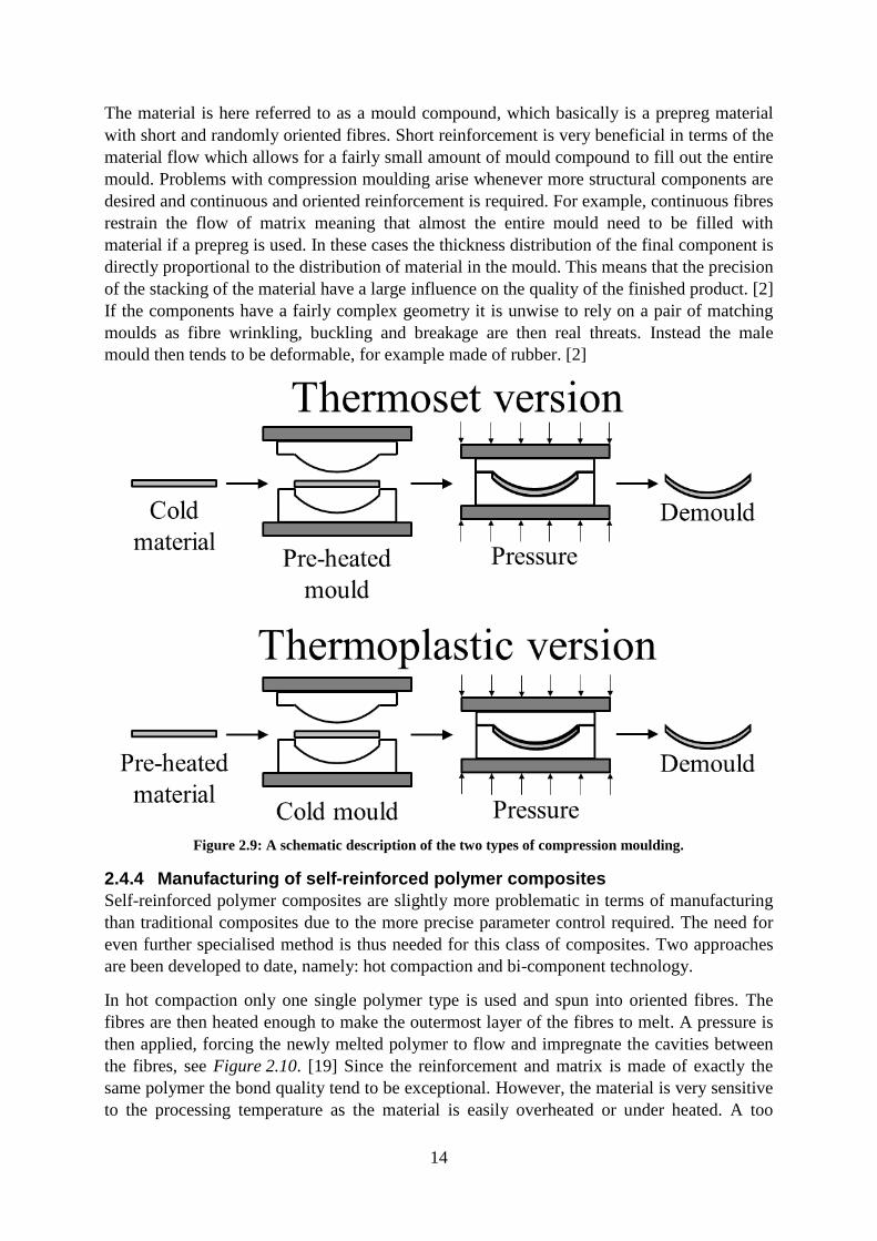
plastic that is used as a basis for the raw material, the heating is carried out differently. A

thermoplastic is commonly pre-heated before it is place in the mould, while the mould itself is

kept cooled to enable short in-mould times, see Figure 2.9. For a thermoset the completely

opposite procedure is common as no curing is desirable prior to the forming, hence the mould

is heated and no pre-heating is performed, see Figure 2.9. The in-mould times thus tend to be

longer for thermoset components. However, the three quantities: time, temperature and

pressure are strongly related throughout the process. If one of these is changed at least one of

the others have to change as well in order to preserve the quality of the product. In this way

one could for example lower the processing time by increasing the pressure and/or

temperature, see Figure 2.8. For example, consider the two points 𝑃1 and 𝑃2 correspond to

two sets of processing parameters. As can be seen 𝑃1 resembles a process with a low pressure

and temperature acting for a long time. However, by increasing the pressure and temperature,

as in 𝑃2, the in-mould time can be reduced.

Figure 2.8: Graphical interpretation of the relationship between the three parameters: time, pressure and

temperature. The arrows indicate the direction of positively increasing parameters.

14

The material is here referred to as a mould compound, which basically is a prepreg material

with short and randomly oriented fibres. Short reinforcement is very beneficial in terms of the

material flow which allows for a fairly small amount of mould compound to fill out the entire

mould. Problems with compression moulding arise whenever more structural components are

desired and continuous and oriented reinforcement is required. For example, continuous fibres

restrain the flow of matrix meaning that almost the entire mould need to be filled with

material if a prepreg is used. In these cases the thickness distribution of the final component is

directly proportional to the distribution of material in the mould. This means that the precision

of the stacking of the material have a large influence on the quality of the finished product. [2]

If the components have a fairly complex geometry it is unwise to rely on a pair of matching

moulds as fibre wrinkling, buckling and breakage are then real threats. Instead the male

mould then tends to be deformable, for example made of rubber. [2]

Figure 2.9: A schematic description of the two types of compression moulding.

2.4.4 Manufacturing of self-reinforced polymer composites

Self-reinforced polymer composites are slightly more problematic in terms of manufacturing

than traditional composites due to the more precise parameter control required. The need for

even further specialised method is thus needed for this class of composites. Two approaches

are been developed to date, namely: hot compaction and bi-component technology.

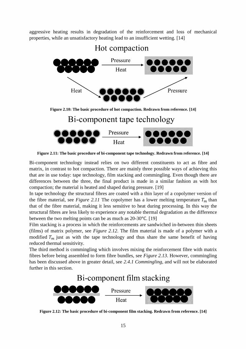
In hot compaction only one single polymer type is used and spun into oriented fibres. The

fibres are then heated enough to make the outermost layer of the fibres to melt. A pressure is

then applied, forcing the newly melted polymer to flow and impregnate the cavities between

the fibres, see Figure 2.10. [19] Since the reinforcement and matrix is made of exactly the

same polymer the bond quality tend to be exceptional. However, the material is very sensitive

to the processing temperature as the material is easily overheated or under heated. A too

15

aggressive heating results in degradation of the reinforcement and loss of mechanical

properties, while an unsatisfactory heating lead to an insufficient wetting. [14]

Figure 2.10: The basic procedure of hot compaction. Redrawn from reference. [14]

Figure 2.11: The basic procedure of bi-component tape technology. Redrawn from reference. [14]

Bi-component technology instead relies on two different constituents to act as fibre and

matrix, in contrast to hot compaction. There are mainly three possible ways of achieving this

that are in use today: tape technology, film stacking and commingling. Even though there are

differences between the three, the final product is made in a similar fashion as with hot

compaction; the material is heated and shaped during pressure. [19]

In tape technology the structural fibres are coated with a thin layer of a copolymer version of

the fibre material, see Figure 2.11 The copolymer has a lower melting temperature 𝑇𝑚 than

that of the fibre material, making it less sensitive to heat during processing. In this way the

structural fibres are less likely to experience any notable thermal degradation as the difference

between the two melting points can be as much as 20-30°C. [19]

Film stacking is a process in which the reinforcements are sandwiched in-between thin sheets

(films) of matrix polymer, see Figure 2.12. The film material is made of a polymer with a

modified 𝑇𝑚 just as with the tape technology and thus share the same benefit of having

reduced thermal sensitivity.

The third method is commingling which involves mixing the reinforcement fibre with matrix

fibres before being assembled to form fibre bundles, see Figure 2.13. However, commingling

has been discussed above in greater detail, see 2.4.1 Commingling, and will not be elaborated

further in this section.

Figure 2.12: The basic procedure of bi-component film stacking. Redrawn from reference. [14]

16

Figure 2.13: The basic procedure of bi-component commingling. Redrawn from reference. [14]

2.5 Shape distortion When dealing with composite materials rather than traditional engineering materials like

metals, several phenomena become increasingly more important and need to be accounted for.

One of these is the concept of shape distortion which arises during the stages of

manufacturing and secondary processing. It describes the tendencies of the material to alter its

geometry as a result of the processing. Generally it is said that shape distortions are comprised

out of three major contributions, namely linear shrinkage, warping and spring-in. [20] Out of

these three, the two latter are of greater importance as they involve changes in the actual

shape and not only the geometrical dimensions alone, see Figure 2.14. The two represent

different phenomena as warping refers to alterations of the shape of flat plates and sections

while spring-in involves changes of angled sections. However, mutual to them both are that

their effects can be derived back to relaxation of residual stresses due to non-constrained

deformation.

Figure 2.14: The three types of shape distortion, linear shrinkage, warping and spring-in.

If the discussion of residual stresses is restricted to composite materials with aligned

continuous reinforcements the stresses can be characterised in three general classes. [21] [22]

Firstly, stresses that act within individual plies are referred to as microstresses which are

formed due to differences in thermal propertied between the constituent. Secondly, stresses

in-between plies are called macrosstresses and are the consequences of anisotropies in the

material as the properties in different directions may vary from ply-to-ply. Lastly, “global” or

“through-the-thickness” stresses are possibly present in the laminate. These are the cause of

gradients of, for example, moisture content and temperature resulting in a non-homogeneous

distribution of these parameters along the thickness direction. Typically a parabolic shaped

distribution can be observed as the resulting global stress response. [21] [22]

The formation of residual stresses in a composite is a process of complex nature and is

dependent on a large number of different factors. These are ranging from various processing

and manufacturing related parameters, like temperatures and pressures, to the properties of the

used matrix and reinforcements. To limit the discussion of residual stresses and shape

17

distortions even further, composite materials with thermoplastic matrices will be the main

focus from now on. Thermosets composites will only be considered to some extent.

2.5.1 Thermal properties of the constituents

A composite material system is a mix of several different materials on a macroscopic scale

with the intent to suppress undesired properties as mention above. It is however rather

uncommon for the different components to have the same thermal properties, with the

coefficient of thermal expansion (CTE) being one example. For a fibre reinforced plastic

(FRP) the CTE can be substantially different between the reinforcements and matrix. This

means that most composite materials experience an uneven expansion between the

constituents resulting in the formation of residual stresses. Apart from this most fibres also

suffer from having dissimilar CTE in the axial direction as in the radial direction, and thus

leading to even further stresses [2].

It should be noted that the CTE is governed by the polymer molecule’s freedom to move and

is thus dependent on crystallinity and temperature. The possibility of expansion is enhanced

by greater possibility of movement and thus the CTE increases with increasing molecular

mobility. In a similar manner the CTE increases more rapidly with temperature as 𝑇𝑔 is

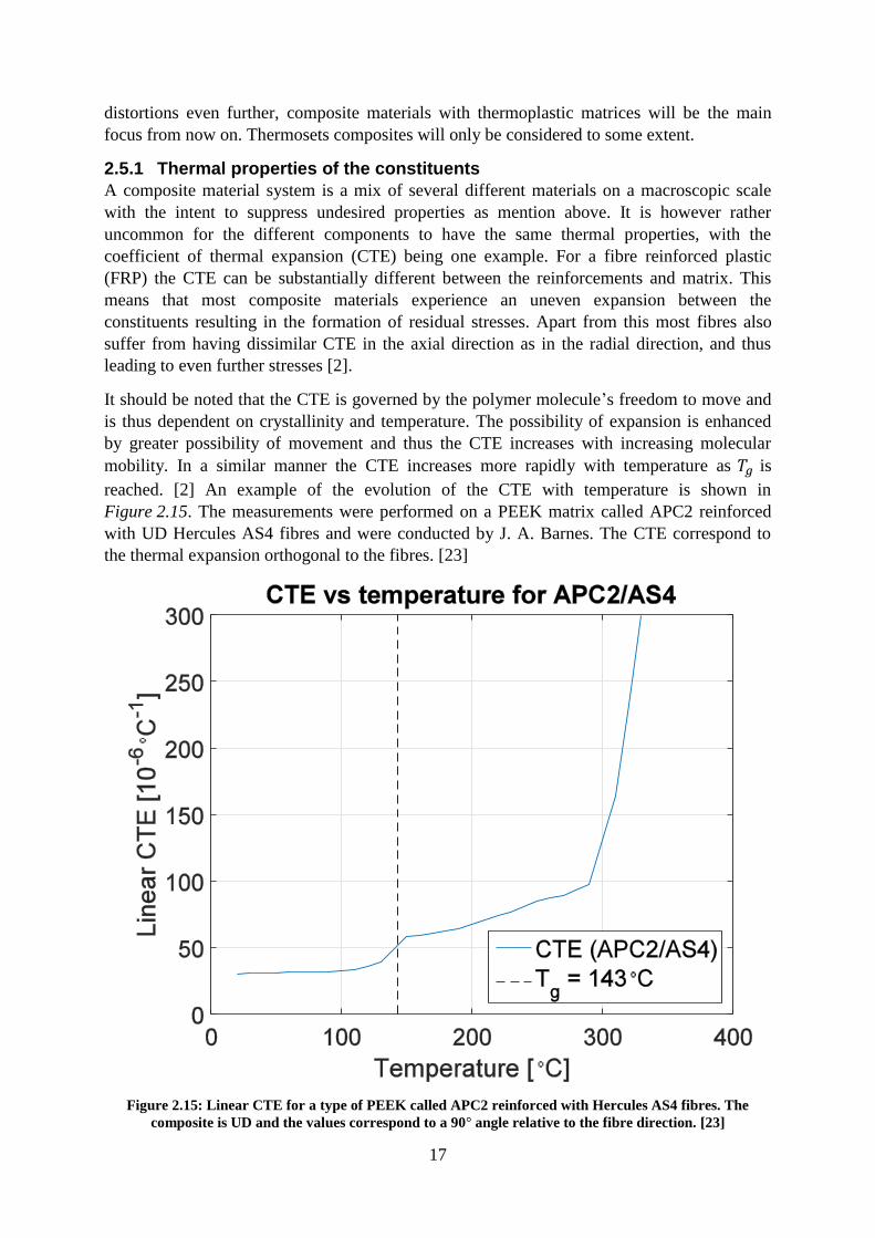
reached. [2] An example of the evolution of the CTE with temperature is shown in

Figure 2.15. The measurements were performed on a PEEK matrix called APC2 reinforced

with UD Hercules AS4 fibres and were conducted by J. A. Barnes. The CTE correspond to

the thermal expansion orthogonal to the fibres. [23]

Figure 2.15: Linear CTE for a type of PEEK called APC2 reinforced with Hercules AS4 fibres. The

composite is UD and the values correspond to a 90° angle relative to the fibre direction. [23]

18

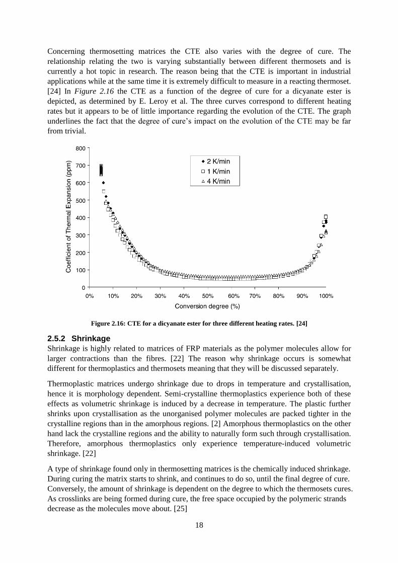
Concerning thermosetting matrices the CTE also varies with the degree of cure. The

relationship relating the two is varying substantially between different thermosets and is

currently a hot topic in research. The reason being that the CTE is important in industrial

applications while at the same time it is extremely difficult to measure in a reacting thermoset.

[24] In Figure 2.16 the CTE as a function of the degree of cure for a dicyanate ester is

depicted, as determined by E. Leroy et al. The three curves correspond to different heating

rates but it appears to be of little importance regarding the evolution of the CTE. The graph

underlines the fact that the degree of cure’s impact on the evolution of the CTE may be far

from trivial.

Figure 2.16: CTE for a dicyanate ester for three different heating rates. [24]

2.5.2 Shrinkage

Shrinkage is highly related to matrices of FRP materials as the polymer molecules allow for

larger contractions than the fibres. [22] The reason why shrinkage occurs is somewhat

different for thermoplastics and thermosets meaning that they will be discussed separately.

Thermoplastic matrices undergo shrinkage due to drops in temperature and crystallisation,

hence it is morphology dependent. Semi-crystalline thermoplastics experience both of these

effects as volumetric shrinkage is induced by a decrease in temperature. The plastic further

shrinks upon crystallisation as the unorganised polymer molecules are packed tighter in the

crystalline regions than in the amorphous regions. [2] Amorphous thermoplastics on the other

hand lack the crystalline regions and the ability to naturally form such through crystallisation.

Therefore, amorphous thermoplastics only experience temperature-induced volumetric

shrinkage. [22]

A type of shrinkage found only in thermosetting matrices is the chemically induced shrinkage.

During curing the matrix starts to shrink, and continues to do so, until the final degree of cure.

Conversely, the amount of shrinkage is dependent on the degree to which the thermosets cures.

As crosslinks are being formed during cure, the free space occupied by the polymeric strands

decrease as the molecules move about. [25]

19

2.5.3 Stress free temperature

Solid amorphous thermoplastics are said to be in either a glassy state or rubbery state

depending on the current temperature of the material. [2] For temperatures below 𝑇𝑔 the

polymer is in its glassy state and the materials are governed by a thermoelastic nature, i.e.

experience an elastic behaviour when subjected to thermal loads. If the temperature is further

increased above 𝑇𝑔 the polymer instead enters the rubbery, representing a state of

viscoelasticity. In this region, relaxation of thermally induced residual stresses is possible due

to the viscoelastic behaviour. However, for this to happen effectively the cooling rate need to

be sufficiently low to allow for such. Any stresses present in the material as it is cooled down

below 𝑇𝑔 are stored or “frozen-in” in the material assuming a completely amorphous

thermoplastic. When dealing with this the concept of “stress free temperature” (SFT) can be

used which represents the temperature below which no relaxation of thermal stress can occur.

Below this temperature, additional temperature drops lead to the formation of stresses that are

not possible to be decreased by relaxation. The lower the operating temperature, relative to

the SFT, the larger the magnitude of these stresses in the thermoelastic region. For amorphous

thermoplastics the SFT is thus in the proximity of 𝑇𝑔. If the thermoplastic is instead semi-

crystalline the SFT is rather in the vicinity of 𝑇𝑐. Crystals are starting to form at around this

temperature and due to the load-bearing capacity of these, so are the residual stresses. Once

again the cooling rate is of importance as the formation of crystals is governed by this. To

reduce the residual stresses formed by the crystallites a higher cooling rate is beneficial since

the degree of crystallinity is kept low. However, this increases the amorphous regions in the

material in which the residual stresses can be relaxed more efficiently for lower cooldown

rates. In this case it is thus beneficial to have both a rapid and slow cooldown at the same time.

The two contributions from the crystals and amorphous regions counteract each other and the

net effect cannot be determined on a general basis but varies between the different

thermoplastics. Relations connecting the crystallinity kinetics and the viscoelastic behaviour

of the material are here needed for further analyses. [21] [22]

2.5.4 Through-thickness variations

Residual stresses, and thus shape distortions, can be formed by non-homogeneous through-

thickness distributions of temperature, cooling rate and fibre content, for example. A

component situated in an environment where the operating temperature is changing, can

experience a gradient in temperature through the thickness. Due to this, a non-homogeneous

deformation field is introduced in the material resulting in residual stresses. However, if the

surrounding temperature is changing slowly or being constant there will be time for the heat

to be distributed evenly. Hence, the stresses are allowed to be relaxed or not even being

generated in the first place. [21]

Cooling rate is of much more importance, at least for materials containing semi-crystalline

thermoplastics. As mentioned above a high cooling rate leads to a lower degree of

crystallinity and thus less crystallisation induced shrinkage and residual stresses. These are

then stored in the material as the temperature drops below the SFT. [21]

Lastly, the distribution of reinforcements in the material will affect the residual stress field. In

this case the distribution of CTE of the material, from a global perspective, will change with

the thickness and thus create uneven formations of stresses. [26]

For a thermoset there is one other parameter to keep track of, as mentioned above, whose

gradient is of importance, namely the degree of cure. As both the CTE and the chemical

20

shrinkage is dependent on this uneven expansions/contractions may arise throughout the

thickness resulting in residual stresses. [26]

2.5.5 Stretching of fibres

It is known that manufacturing of polymeric fibres rely on the fact that the used methods alter

the microstructure of the material as the molecules become oriented. A study involving the

identical type of SrPET weaves as used in the present study has been conducted by L. Jerpdal

and M. Åkermo. [6] Their focus was to investigate the correlation between the mechanical

properties of the material and stretching as well as shrinkage of the PET fibres. The results

showed that stretching of the fibres above 𝑇𝑔 during pre-heating resulted in enhanced

mechanical properties while shrinkage was of less significance regarding these. This indicated

that the degree of orientation of the polymers could be increased for the used materials in a

similar fashion as during the post-drawing processing.

The extra stretching possibly yields more potential shrinkage at elevated temperatures as the

molecular chains can relax to a larger extent. For a manufacturing method such as

compression moulding, where stretching of the reinforcement could be possible, this may be a

real threat. This is especially true if the stretching is non-uniform.

2.6 Measurement techniques Measurements are a fundamental part of every branch of science as it is a way of quantifying

certain aspects of a made observations. Great care should therefore be taken to perfect the

measurement techniques as they inherently govern the quality of the final outcome of a study,

for example. To be able to utilise the full potential of a particular method it is good praxis to

understand the underlying physics and principles.

2.6.1 Triangulation

Triangulation is a procedure based on trigonometry in which the position of a point is

determined by solely relying on measurements of angles. In order for the method to work in a

2D situation a total of three points are needed, out of which two are fixed and one is the target

to be measured, see Figure 2.17. These three points together form a triangle, hence the name

triangulation. A line is then formed between the two fixed points, referred to as the baseline,

which are situated a known distance 𝑑 apart. The angle 𝜃 between the baseline and a line

stretched between one of the fixed points and the target is then recorded. This allows for the

distances 𝑥1 or 𝑥2 to be calculated, and thus the position of the target has been determined.

Figure 2.17: Illustration of triangulation together with schematic set up of a 3D laser scanner.

21

2.6.2 3D laser scanning

3D laser scanning is a measurement technique that can be used to create a digitalised

representation of an object. This is achieved by scanning the objects surfaces with the help of

laser beams that are projected onto the faces as either lines or points. A set of cameras then

register the angles between the cameras and the projections relative to the corresponding set

of baselines for the cameras and the laser emitters, see Figure 2.17. Through triangulation a

set of points are then created relative a to reference point, which may be situated inside of the

scanner itself. This generates a point cloud representation of the surfaces which can be used to

form a CAD model by means of interpolated triangular mesh in-between the points.

Laser scanners can be static, fixed to a rig, or dynamic, for example a handheld version.

Depending on the type, a slightly extended procedure than that described above may need to

be implemented. As handheld scanners are dynamic and constantly in motion during the

scanning, so is the reference point which needs to be tracked throughout the whole procedure.

This is typically done by adding reflective stickers on surfaces in the vicinity of the object or

directly on the object to be scanned itself. It is also possible to determine the position and

orientation of the scanner by means of external devices, based on lasers or cameras.

3 Materials In the present study four different materials were used during testing, all of which were

commingled weaves with matrix fibres based on amorphous LPET (low melting

poly(ethylene terephthalate)) with a density of 1.38 g/cm3. Out of these four, one was a 4/

1 warp/weft directed plain weave reinforced with HTPET (high tenacity poly(ethylene

terephthalate)) fibres. As 80% of the fibres are aligned along the longitudinal direction, the

supplier refers to it as UD. The density of the HTPET is the same as for the LPET, namely

1.38 g/cm3. Furthermore, the fibre weight content is 50%, and thus the fibre volume content

alike, as the densities of the constituents are equal. This leads to total surface density of 555

g/m2 for the weave with the present level of packing [18].

The remaining three were 2/2 warp/weft directed twill weaves reinforced with HTPET, glass

and carbon fibres respectively. The density of the HTPET is, again, 1.38 g/cm3

while

characteristic values for glass and carbon are 2.6 g/cm3

and 1.8 g/cm3

as specified by the

supplier. Moreover, the fibre weight content for the three materials are 50%, 57% and 54%,

respectively, while the corresponding volume content are 50%, 42% and 47%. The fibre

volume content for the carbon/LPET material was not specified by Comfil ApS, but rather

estimated with the rule of mixture. In relation to the plain weave, the twill weaves are more

densely packed resulting in surface densities of 710, 750 and 500 g/m2

for the HTPET, glass

and carbon textiles. [18]

The material data for the four weaves are summaries in Table 3.1 below.

22

Table 3.1: Material data corresponding to the four weaves used in the study [18]. Note that the volumetric

densities for the glass and carbon fibre are only approximate values. Furthermore, the fibre volume

fraction for the carbon/LPET twill weave has been determined through the rule of mixture.

Fibre Matrix Weave

architecture

Fibre

density

[g/cm3]

Matrix

density

[g/cm3]

Areal

density

[g/m2]

Fibre

weight

fraction

Fibre

volume

fraction

Product

number

HTPET LPET Plain (4/1) 1.38 1.38 555 0.50 0.50 30113-4

HTPET LPET Twill (2/2) 1.38 1.38 710 0.50 0.50 30112-4

Glass LPET Twill (2/2) 2.60 1.38 750 0.57 0.42 30001-3

Carbon LPET Twill (2/2) 1.80 1.38 500 0.54 0.47 30013-8

4 Method In the following sections the methodologies used during the experimental parts of the study

are presented. To begin with the manufacturing of the SrPET panels is described, both in

terms of process parameters and used equipment. Thereafter, the secondary processing steps

are presented in a similar fashion, followed by a description of the employed measuring- and

data evaluation techniques.

4.1 Manufacturing of test specimens Before the test specimens could be manufactured, the material needed to be dried for some

time as PET is sensitive to hydrolysis, see 2.2.1.2 PET. Therefore, a Weiss DU11 160 climate

chamber was used to create an atmosphere with a temperature of 50°C and a relative humidity

of 15% in which the samples were kept. The PET was left to dry in the climate chamber for a

minimum of 24 hours to ensure a low enough moisture content in the material. All of this was

carried out in accordance with the specifications provided by the supplier. [18]

Figure 4.1: The ideal shape of the test specimens along with the reference line from which the main fibre

angle is defined.

Once the PET material had been dried the manufacturing of the test specimens could

commence. The ideal geometry of the components is presented Figure 4.1. It corresponds to a

“V” with an opening angle of 90°, a rounded tip and two horizontal flanges on either ends.

There is a constant thickness of 2 mm throughout the component and the inner and outer radii

23

of the tip are 2 mm and 4 mm respectively. A set of components was created with different

degrees of fibre stretching, weave architectures and main fibre angles to test the impact of

these parameters. The specifications of the manufactured specimens, and the corresponding

amount of each, are presented in Table 4.1. In addition to HTPET fibres, components

reinforced with glass- and carbon fibres were also studied to allow for comparisons between

the three. The glass- and carbon fibre components were however kept un-stretched as these do

not allow for any notable elongation in contrast to the HTPET fibres.

Table 4.1: Information regarding the manufactured specimens.

Material Fibrous form Main fibre angle

[°]

Stretching

[%]

Amount of

layers

Amount of

specimens

HTPET/LPET

Plain 4/1

(warp/weft)

0 0 4 5

0 10 4 5

0 13 4 5

Twill 2/2

(warp/weft)

0 0 4 5

0 10 4 5

0 13 4 5

45 10 4 5

45 13 4 5

Carbon/PET Twill 2/2

(warp/weft) 0 0 7 5

Glass/PET Twill 2/2

(warp/weft) 0 0 6 5

The main fibre angle is defined as the angle between the warp threads of the fabrics and a

reference line, shown in Figure 4.1. This line runs along a cross section of the panels that is

parallel to the two shorter sides.

Figure 4.2: The two halves of the mould used during the manufacturing of the V-shaped panels.

Compression moulding was the choice of manufacturing method due to the very beneficial

shape of the specimens and thus a two-part mould in aluminium was used, see Figure 4.2. The

two halves are roughly 160 mm x 270 mm x 70 mm and 160 mm x 325 mm x 70 mm

respectively in terms of their extreme ends. The stretching of the structural HTPET fibres was

introduced during the mould closure as the material was forced down into the V-shaped cavity

with a pressing depth of approximately 45 mm, see Figure 4.2. To accomplish the desired

level of stretching a custom made rig, as shown in Figure 4.3, was utilised. It consisted of two

24

threaded rods, two struts and two clamping devices, see Figure 4.3 and 4.4. Long strips of the

material were then cut to size and wound around the rods, which were kept at a predetermined

distance from each other with the help of the struts. By altering the distance between the two

rods the needed length of the initial material was altered, hence the degree of stretching in the

material could be controlled. The rods were then enclosed by the clamps which were shut and

tightened with bolts, keeping the material in place and preventing slack. To reduce the

necessary force needed to stretch the fibres, the material, together with the whole stretching

assembly, was pre-heated in a Heraeus UT 5050 E oven to 110°C with an average heating rate

of 26.7°C/min. The pre-heating also served to render the results comparable with those in an

earlier study. Namely a study conducted by L. Jerpdal and M. Åkermo [6], dealing with the

influence of fibre stretching on the mechanical properties of the same material systems.

Simultaneously, the two tool halves were also pre-heated in the same oven to the same

temperature, 110°C. Thereafter a layer of Teflon release film with a thickness of 0.25 mm was

placed on either side of the material before the whole stretch rig was placed in-between the

two mould halves. The entire stack was then moved to a Fontijne Presses LabEcon 600 heated

hydraulic press with two metal pressure plates. These were pre-heated to 250°C to yield a

quick final heating of the material, and mould stack, to the target temperature of 215°C. The

hydraulic press was then closed with a permissible maximum force of 100 kN to allow for a

rapid mould closure. However, just as the mould halves were about to start exerting a pressure

on the material, the allowable upper limit on the applied force was decreased to 65 kN. This

limit had been calculated to yield a consolidation pressure of 1.5 MPa which were maintained

until demoulding. It took roughly 4 minutes and 30 seconds for the material to reach 215°C at

which point the temperature of the pressure plates also had been decreased to 215°C. The

average heating rate was approximately 23.3°C/min during this stage. At this temperature the

material was left to consolidate for 9 minutes before the cooling phase was started. Water

cooling was then applied to the two pressure plates for 10 minutes resulting in an average

cooling rate of 17°C/min. This was followed by a 1 minute and 30 seconds long stage of air

cooling in which the temperature was not notably changed. It merely served to flush out the

remaining water in the piping. In total the whole process lasted for about 25 minutes. A

graphical illustration of the process is shown in Figure 4.7.

Figure 4.3: Picture showing the stretch rig. The shown parts are the clamping devices (1), the two threded

rods (2) and the struts (3).

25

Figure 4.4: Top view of the assembled stretch rig in use. The restrained material in the rig is the SrPET

twill fabric which has been preheated to 110°𝐂. Note that the material has shrunk along the vertical

direction in the picture.

When the SrPET material is heated above 80°C a fairly substantial shrinkage is experienced in

the LPET matrix fibres, see Figure 4.6. Therefore, when the components with un-stretched

fibres were manufactured the pre-heating phase of the material, and the tool, had to be

excluded due to the absence of the stretch rig. The material was then instead heated to 215°C

directly in the heated press, in which the material shrinkage could be kept at bay with the

applied pressure. The average heating rate of the material was here approximately 28.5°C/min.

The manufacturing process thus needed to be altered, as the initial heating phase up to 215°C

required an additional 2 minutes. However, the consolidation time was still kept the same, i.e.

9 minutes. Furthermore, the increased force applied during the initial phase was no longer

necessary. The two different set point programmes, as provided to the heated press during the

manufacturing, are presented as graphs in Figure 4.5. For this slightly modified process the

components spent a total time of 27 minutes in the mould.

Figure 4.5: Process parameter set point values during manufacturing.

26

Figure 4.6: Four equally sized pieces (20 cm x 20 cm) of SrPET, two pieces of the twill fabric (to the left)

and two pieces of the plain fabric (to the right). One from each set was heated to above 80°𝐂 while the

others were kept as references. The heat triggered shrinkage in the matrix fibres causing the fabrics to

curl.

Figure 4.7: Schematic description of how the components were manufactured through compression

moulding.

4.2 Secondary processing When all of the panels had been manufactured they were sent off to have their bottom exterior

surface, see Figure 4.8, scanned with a 3D laser scanner for further analysis, see 4.3

Measurements of shape distortions. After the scanning was completed the panels were sawed

into three equally sized pieces; one to be heated, one to be treated with both heat and

chemicals, and one to act as a reference. Any excess material was sanded off with fine grained

sandpaper and the edges were slightly rounded off. The thicknesses and spring-in angles of

the components were recorded with a calliper and a 3D laser scanner, respectively, both prior

to and after the respective secondary treatment.

Figure 4.8: Definition of the bottom exterior surface which is highlighted in a dark grey colour.

27

4.2.1 Heat treatment

The heat treatment of the panels involved a 40 minutes long exposure to 90°C before being

allowed to cool back down to room temperature. The procedure was designed in accordance

to a standard surface treatment process of a thermoplastic component. During the test a

Heraeus UT 5050 E oven was utilised in which 18 specimens were placed at a time, oriented

as shown in Figure 4.9.

Figure 4.9: Orientation of the panles during the 3D laser scanning and the different secondary processing

procedures.

4.2.2 Chemical treatment

The exterior of the panels were treated with a Glasurit 352-91 thinner to represent a common

surface coating of a thermoplastic component. Firstly the chemical was sprayed onto the

surfaces to ensure an initial and evenly distributed wetting. Absorbent pads soaked with the

thinner were then left on top of the components for 10 minutes to increase the duration of the

chemical expositor. This was done to simulate the effect of the left out binder used in the real

coating process. The pads were then removed and the chemicals were allowed to evaporate

during a 10 minutes long flash off period. After this stage the panels were heated in the same

manner as described in 4.2.1 Heat treatment, i.e. in an oven at 90°C for 40 minutes. Here a

Memmert UFE 500 oven was used.

4.3 Measurements of shape distortions Measurements of the panels were conducted by scanning their bottom exterior surfaces to

investigate whether they had been afflicted by any spring-in, see Figure 4.8. The

measurements were performed using a handheld Creaform HandySCAN 3D 700 laser scanner

with a resolution of 80 μm. From the scanning a point cloud representation of the surfaces

were generated in the form of stl-files, see 2.6.2 3D laser scanning and Figure 4.10, which

where post-processed in the CAD software CATIA V5 R24. No alignment of the specimens

was performed during the scanning meaning that the position of the point clouds, in relation

to the reference coordinate system, was completely arbitrary. To be able to extract the desired

angles from a cross section parallel to the short edges of the specimens, an approximate

artificial alignment had to be performed. Therefore, a set of points, lines and planes were

created in CATIA V5 R24 on top of the measured panel surfaces, see Figure 4.11. By doing

this in an ordered and iterative fashion a plane, approximately parallel to the short edges, was

generated and the sought cross section could be acquired. The measured surface was cut along

the newly created plane and 100 equidistant points where added to either of the two tilted side

of the V-shaped panels. These points where then exported as a list of three-dimensional

coordinates and imported in MATLAB R2014b for further analysis. Vectors were introduced

in-between each pair of adjacent points to create a piecewise linear approximation of the cross

section.

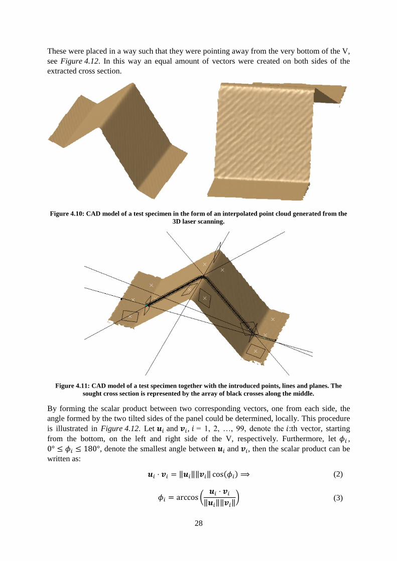
28

These were placed in a way such that they were pointing away from the very bottom of the V,

see Figure 4.12. In this way an equal amount of vectors were created on both sides of the

extracted cross section.

Figure 4.10: CAD model of a test specimen in the form of an interpolated point cloud generated from the

3D laser scanning.

Figure 4.11: CAD model of a test specimen together with the introduced points, lines and planes. The

sought cross section is represented by the array of black crosses along the middle.

By forming the scalar product between two corresponding vectors, one from each side, the

angle formed by the two tilted sides of the panel could be determined, locally. This procedure

is illustrated in Figure 4.12. Let 𝒖𝑖 and 𝒗𝑖, 𝑖 = 1, 2, …, 99, denote the 𝑖:th vector, starting

from the bottom, on the left and right side of the V, respectively. Furthermore, let 𝜙𝑖 ,

0° ≤ 𝜙𝑖 ≤ 180°, denote the smallest angle between 𝒖𝑖 and 𝒗𝑖, then the scalar product can be

written as:

𝒖𝑖 ⋅ 𝒗𝑖 = ‖𝒖𝑖‖‖𝒗𝑖‖ cos(𝜙𝑖) ⟹ (2)

𝜙𝑖 = arccos (𝒖𝑖 ⋅ 𝒗𝑖

‖𝒖𝑖‖‖𝒗𝑖‖) (3)

29

where “‖⋅‖” represents the three-dimensional Euclidian norm of the vectors. From this the

opening angle could be determined as a function of the index 𝑖, see Figure 4.13.

Figure 4.12: Demonstration of the method used to determine the angle between the two tilted sides of the

panels.

This represents how the opening angle varied along the cross section of the component from

the bottom to the end of the tilted sides slightly below the start of the flanges. The initial part

of the graph, typically the region 𝑖 = [1, 13] , was discarded as it represented the curved

bottom and thus did not contain any useful information. In other words, the graph was started

where the circular tip merges with the tilted sides of the V, see Figure 4.14. The same was

done at the other end of the tilted side, i.e. the flanges were removed. Here everything after,

and including, the typical value of index 𝑖 = 96 was neglected. The generated graphs were

very noisy so to extract the necessary data a linear function was fitted to the data set, see

Figure 4.13.

Figure 4.13: Opening angle as a function of the index 𝒊.

30

It was i.e. assumed that the opening angle varied linearly from top to bottom. The opening

angle of the component was then taken as the value at the left end of the linear fit. By

subtracting the initial angle the spring-in angle could be acquired. The initial angle was taken

as the angle in the female mould, i.e. 90°. However, it should be noted that the recorded

spring-in after any of the secondary processing steps also include the manufacturing induced

spring-in. Thus, to acquire the additional angular change caused by these the corresponding

spring-in angle after manufacturing needs to be subtracted from the values presented in the

5.1.2 Measured shape distortions section. The warping distribution was quantified as the

maximum warping, meaning the angular difference between the two extremes of the tilted

sides, see Figure 4.14. The lower angle of the two corresponds to the spring-in, which was

now known, and the upper angle could be acquired in a similar fashion. For this the value at

the right end of the linear fit was taken to represent the opening angle at the top of the

component. From these two angles the difference was calculated and then divided by two,

meaning that the warping was assumed to be symmetric on both sides. As the warping was

calculated in a similar manner as the spring-in angle it goes with the same warning regarding

the presented results below for the secondary treated components. The manufacturing induced

maximum warping needs to be subtracted to yield the angular changes due to the secondary

processing itself.

Figure 4.14: Definition of a positive spring-in and maximum warping.

Tests were also conducted in which the thicknesses of the specimens were determined

approximately with the help of the 3D laser scanner. Both the inner and outer surfaces were

then measured of a set of predetermined specimens, one made of each of the four materials

used, see Table 3.1. The surfaces were then approximated with planes and the orthogonal

distance between them measured at several locations. These measurements are summarised in

Table 5.3.

31

5 Results In the following sections the various results and measurements that were recorded during the

experiments are presented. It starts with a section dealing with the quality of the components

followed by a section listing the observed spring-in and maximum warping angles.

5.1.1 Quality of the manufactured components

5.1.1.1 Thickness after manufacturing

In Table 5.1 below, the thicknesses of the sawed reference components are stored. It is

evident that the target thickness of 2 mm was not reached; let alone the desire of having a

constant thickness throughout the components. According to the table, components

manufactured with a non-zero degree of fibre stretching ended up with a substantial variation

in thickness between the two sides. The reason for the large relative differences in thickness

between the twill and plain components, as evident in Table 5.1, is explained by the number

of layer used. During the manufacturing of the plain components a too small amount of fabric

layers were used to reach the desired limit. Therefore, any difference in the absolute values of

the measured shape distortions between the two material types should not be scrutinised to

thoroughly. Table 5.1: Determined mean values of the thicknesses of the two tilted edges of the panels. The thickest

side was defined as the right side of the components.

Material Thickness (left)

[mm]

Thickness (right)

[mm]

HTPET-P0-0 1.24 ± 0.05 1.28 ± 0.06

HTPET-P0-10 1.30 ± 0.04 1.48 ± 0.08

HTPET-P0-13 1.24 ± 0.05 1.45 ± 0.05

HTPET-T0-0 1.69 ± 0.02 1.71 ± 0.02

HTPET-T0-10 1.58 ± 0.02 1.97 ± 0.04

HTPET-T0-13 1.55 ± 0.05 1.97 ± 0.04

HTPET-T45-10 1.59 ± 0.05 1.91 ± 0.10

HTPET-T45-13 1.75 ± 0.05 2.01 ± 0.04

Carbon-T0-0 2.10 ± 0.00 2.16 ± 0.13

Glass-T0-0 1.76 ± 0.04 1.82 ± 0.03

5.1.1.2 Thickness changes after secondary processing

Almost no variations in thickness could be recorded as a result of the pure heat- and chemical

treatments with the accuracy achieved with the used calliper. Therefore, the reader is spared

with the delight of having to plough through most of the additional measurements; only the

values for the glass- and carbon fibre components are presented, see Table 5.2. As can be seen

in the table the carbon fibre reinforced panels have not been affected by either of the heat and

chemical treatments to any noteworthy degree. The same goes for the heat treated glass fibre

reinforced components. However, the chemical treatment had a larger impact on the glass

fibre composites.

32

Table 5.2: Thickness change in the carbon and glass fibre component after the heat and chemical

treatment. The changes in the SrPET components were all within the corresponding uncertainty limits

and are thus not presented. The thickest side was defined as the right side of the components.

Material

Heat treated Chemically treated

Thickness

change (left)

[mm]

Thickness

change (right)

[mm]

Thickness

change (left)

[mm]

Thickness

change (right)

[mm]

Carbon-T0-0 0.03 ± 0.03 0.03 ± 0.02 0.05 ± 0.04 0.07 ± 0.04

Glass-T0-0 0.03 ± 0.03 0.06 ± 0.02 0.11 ± 0.05 0.11 ± 0.04

5.1.1.3 Thickness estimations using 3D laser scanning

The thicknesses of the four panels that were estimated, with the 3D laser measurements and

the CAD software CATIA V5 R24, are shown in Table 5.3. By comparing these with the

physical measurements acquired with a calliper it can be seen that in most cases there is a

substantial loss of thickness. One exception is however the carbon fibre reinforced PET

component (with the measured thicknesses: 2.1 mm and 2.4 mm) which had its thicknesses

determined with a relatively high accuracy compared to the other. The error limits shown

correspond to the uncertainty introduced as the distance between the two planes were

measured at several different points. The method of determining the thicknesses digitally in

CATIA V5 R24 was a bit crude and likely introduced uncertainties which will be discussed

further in 6.2.8 Transparency of the LPET matrix.

Table 5.3: Thickness measurements of the tilted panel sides. The carbon fibre component was extra thick

as it appears that an extra layer was accidentally added to one of the sides during manufacturing. The

thickest side was defined as the right side of the components.

Material Fibrous form

Calliper measurements 3D scanning

Thickness

(left)

[mm]

Thickness

(right)

[mm]

Thickness

(left)

[mm]

Thickness

(right)

[mm]

HTPET/LPET

Plain 4/1

(warp/weft) 1.2 1.5 0.83 ± 0.10 1.09 ± 0.12

Twill 2/2

(warp/weft) 1.7 1.7 1.04 ± 0.04 1.14 ± 0.08

Carbon/PET Twill 2/2

(warp/weft) 2.1 2.4 2.13 ± 0.02 2.37 ± 0.03

Glass/PET Twill 2/2

(warp/weft) 1.8 1.8 1.25 ± 0.19 1.33 ± 0.14

5.1.1.4 Indentations in the surfaces

Lastly, during manufacturing a strange phenomenon in which long channel-like indentations

appeared on the outer surface of the components, were observed, see Figure 5.1. These arose

around the bottom tip in many of the components with a non-zero fibre stretching and caused

localised thickness reductions. As the upper mould half was pushed down into the cavity of

the bottom half the release film started to wrinkle and created the indentations.

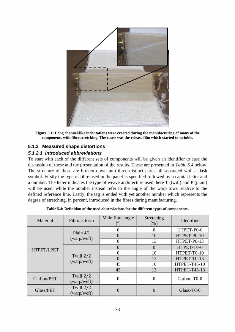
33

Figure 5.1: Long channel-like indentations were created during the manufacturing of many of the

components with fibre stretching. The cause was the release film which started to wrinkle.

5.1.2 Measured shape distortions

5.1.2.1 Introduced abbreviations

To start with each of the different sets of components will be given an identifier to ease the

discussion of these and the presentation of the results. These are presented in Table 5.4 below.

The structure of these are broken down into three distinct parts; all separated with a dash

symbol. Firstly the type of fibre used in the panel is specified followed by a capital letter and

a number. The letter indicates the type of weave architecture used, here T (twill) and P (plain)

will be used, while the number instead refer to the angle of the warp tows relative to the

defined reference line. Lastly, the tag is ended with yet another number which represents the

degree of stretching, in percent, introduced in the fibres during manufacturing.

Table 5.4: Definition of the used abbreviations for the different types of components.

Material Fibrous form Main fibre angle

[°]

Stretching

[%] Identifier

HTPET/LPET

Plain 4/1

(warp/weft)

0 0 HTPET-P0-0

0 10 HTPET-P0-10

0 13 HTPET-P0-13

Twill 2/2

(warp/weft)

0 0 HTPET-T0-0

0 10 HTPET-T0-10

0 13 HTPET-T0-13

45 10 HTPET-T45-10

45 13 HTPET-T45-13

Carbon/PET Twill 2/2

(warp/weft) 0 0 Carbon-T0-0

Glass/PET Twill 2/2

(warp/weft) 0 0 Glass-T0-0

34

Along with the above stated identifier four abbreviations will be defined to ease the references

to the four different sets of components. These are the components directly after

manufacturing (M), after sawing (S), heat treatment (H) and chemical treatment (C), see

Table 5.5.

Table 5.5: Abbreviation used in to denote sets of components based on manufacturing and secondary

processing steps.

Component

type

After

manufacturing

After

sawing

After

heat treatment

After

chemical treatment

Abbreviation M S H C

5.1.2.2 M components

The estimated spring-in and warping angles acquired from the 3D scanning of the panels are

presented in Table 5.6 and 5.7 below and graphically illustrated in Figure 5.2 and 5.3. As can

be seen in Table 5.6 and Figure 5.2a all of the spring-in angles in the components have a

positive mean value. This means that the opening angles decreased. However, the stretched

HTPET-P0 and HTPET-T0 panels experienced a fairly substantial scattering in the induced

angular changes. Their standard deviations are thus large; both increases and decreases in the

opening angle were observed in components within each set!

Table 5.6: Measured spring-in angles for all of the panels. The values corresponding to the H and C

components represents the observed spring-in angles relative the ideal 90° shape rather than the reference

S components. An angular change that strives to close the V-shape is defined as positive.

Material Spring-in [°]

(M)

Spring-in [°]

(S)

Spring-in [°]

(H)

Spring-in [°]

(C)

HTPET-P0-0 1.4 ± 0.1 1.1 ± 0.4 3.1 ± 0.3 1.3 ± 0.3

HTPET-P0-10 0.2 ± 0.9 0.9 ± 1.2 1.1 ± 1.1 0.6 ± 1.6

HTPET-P0-13 0.3 ± 0.8 0.6 ± 0.7 1.2 ± 0.8 0.7 ± 0.7

HTPET-T0-0 1.4 ± 0.2 1.1 ± 0.2 2.4 ± 0.2 0.6 ± 0.3

HTPET-T0-10 0.5 ± 0.6 0.6 ± 0.2 1.9 ± 0.3 0.4 ± 0.2

HTPET-T0-13 0.2 ± 0.6 0.4 ± 0.6 1.6 ± 0.3 0.9 ± 0.7

HTPET-T45-10 0.9 ± 0.1 0.9 ± 0.3 2.3 ± 0.2 1.2 ± 0.6

HTPET-T45-13 1.0 ± 0.3 0.8 ± 0.2 2.0 ± 0.5 0.5 ± 0.2

Carbon-T0-0 0.8 ± 0.2 0.8 ± 0.1 -0.7 ± 0.3 -1.4 ± 0.4

Glass-T0-0 0.5 ± 0.2 0.1 ± 0.5 -5.4 ± 1.1 -5.6 ± 1.3

Table 5.7 and Figure 5.3 indicate that the components tend to have a non-constant opening

angle as a function of the component height. The angular change between the two ends of the

tilted sides, the maximum warping, have negative mean values for all of the M SrPET and the

carbon fibre components. Geometrically, the tilted sides thus bent outwards at the top so that

the V-shape was further opened. The opposite reaction was observed in the glass fibre

component as it had a positive warping, i.e. the sides bent inwards.

5.1.2.3 S components

In the three remaining columns of Table 5.6 and 5.7 the measured spring-in and maximum

warping angles, after the various secondary processing steps, are presented. The same goes

with the rest of the graphs in Figure 5.2 and 5.3. The third columns of the two contain the

35

shape distortion measured in the S components. Mostly the angles measured before and after

sawing lie in the same regions, at least if the corresponding standard deviations are taken into

account. This is also illustrated in Figure 5.2b and 5.3b.

Table 5.7: Measured maximum warping for all of the panels. The values corresponding to the H and C

components represents the observed maximum warping angles relative the ideal 90° shape rather than the

reference S components. An angular change that strives to close the V-shape is defined as positive.

Material Max. warping [°]

(M)

Max. warping [°]

(S)

Max. warping [°]

(H)

Max. warping [°]

(C)

HTPET-P0-0 -1.0 ± 0.2 -0.9 ± 0.3 0.3 ± 0.5 0.7 ± 0.7

HTPET-P0-10 -1.2 ± 0.7 -1.4 ± 0.5 -0.6 ± 0.8 0.3 ± 0.7

HTPET-P0-13 -1.1 ± 0.6 -1.2 ± 0.4 0.1 ± 0.8 0.9 ± 0.7

HTPET-T0-0 -0.6 ± 0.2 -0.5 ± 0.1 -0.1 ± 0.2 0.5 ± 0.4

HTPET-T0-10 -1.6 ± 0.4 -1.5 ± 0.2 -0.8 ± 0.8 0.5 ± 0.5

HTPET-T0-13 -2.4 ± 0.4 -2.2 ± 0.3 -2.1 ± 0.5 -0.8 ± 0.7

HTPET-T45-10 -0.9 ± 0.2 -1.0 ± 0.3 -0.5 ± 0.4 0.4 ± 0.3

HTPET-T45-13 -1.0 ± 0.2 -0.8 ± 0.2 -0.4 ± 0.4 0.1 ± 0.2

Carbon-T0-0 -0.1 ± 0.2 -0.2 ± 0.1 -0.1 ± 0.1 0.4 ± 0.3

Glass-T0-0 0.5 ± 0.2 0.7 ± 0.5 0.1 ± 0.4 -0.1 ± 0.7

5.1.2.4 H components

In the fourth columns from the left in Table 5.6 and 5.7 the measured angular changes

observed in the H components are stored. These values represent the shape distortions relative

the ideal 90° shape, i.e. it is a combination of both the manufacturing induced and heat

treatment induced angular changes. It can be seen that the additional heat expositor further

increased the spring-in angle in the SrPET components, see also Figure 5.2c. The same

cannot be said regarding the glass- and carbon fibre reinforced components which instead

reacted with a decrease in the same angle; a very large change at that in the glass fibre

components. Delamination was also observed at the bottom and in the tilted sides of the

Glass-T0-0 components. The absolute value of the maximum warping decreased for all of the

components so that it was almost completely removed for the un-stretched ones, see also

Figure 5.3c. However, the stretched HTPET-T0 components still experience a fairly large

warping, though still smaller than the reference values.

It was observed that the surface texture of the components became rougher due to the heat

treatment.

5.1.2.5 C components

The results from the C panels are presented in the fifth and final column of Table 5.6 and 5.7

while being graphically illustrated in Figure 5.2d and 5.3d. In a similar fashion as with the H

data the preceding column, the values represent the shape distortions relative the ideal 90°

shape. By comparing the two secondary surface treatments it can be said that the angular

changes are rather different. The observed changes in the mean spring-in in the SrPET

components include both positive and negative values. For example, a decrease in spring-in

was recorded for the HTPET-T0-0, HTPET-T0-10 and HTPET-T45-13 components while it

instead increased in the HTPET-T0-13 and HTPET-T45-10. The Glass-T0-0 and Carbon-T0-0

components reacted in a similar way as the corresponding H components, though with a larger

absolute change. Delamination was observed in the glass fibre components after this

36

experiment as well. In terms of the warping the C components seem to again have been

affected in a random manner. The SrPET and carbon fibre measurement points have been

shifted upwards in the graph, see Figure 5.3d, while the glass fibre point was shifted

downwards. The overall relationship between the warping and the degree of stretching was

not kept for the HTPET-T0 and HTPET-T45 components, relative the reference, during the

shift. The maximum warping now decreased in the HTPET-T45 components with degree of

stretching while it was not dependent on degree of stretching in the case of the HTPET-T0-0

and HTPET-T0-10.

It was observed that the surface texture of the components became rougher due to the

chemical treatment.

Figure 5.2: Measured spring-in angles (graphical representation of Table 5.6). The spring-in angles in the

M components are shown in the upper left graph (a), the S components in the graph to the upper right,

the H components in the graph to the lower left and the C components to the graph to the lower right.

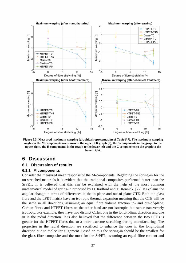
37

Figure 5.3: Measured maximum warping (graphical representation of Table 5.7). The maximum warping

angles in the M components are shown in the upper left graph (a), the S components in the graph to the

upper right, the H components in the graph to the lower left and the C components to the graph to the

lower right.

6 Discussion

6.1 Discussion of results

6.1.1 M components

Consider the measured mean response of the M-components. Regarding the spring-in for the

un-stretched materials it is evident that the traditional composites performed better than the

SrPET. It is believed that this can be explained with the help of the most common

mathematical model of spring-in proposed by D. Radford and T. Rennick. [27] It explains the

angular change in terms of differences in the in-plane and out-of-plane CTE. Both the glass

fibre and the LPET matrix have an isotropic thermal expansion meaning that the CTE will be

the same in all directions, assuming an equal fibre volume fraction in- and out-of-plane.

Carbon fibres and HTPET fibres on the other hand are not isotropic, but rather transversely

isotropic. For example, they have two distinct CTEs, one in the longitudinal direction and one

in in the radial direction. It is also believed that the difference between the two CTEs is

greater for the HTPET fibres due to a more extreme stretching during manufacturing. The

properties in the radial direction are sacrificed to enhance the ones in the longitudinal

direction due to molecular alignment. Based on this the spring-in should be the smallest for

the glass fibre composite and the most for the SrPET, assuming an equal fibre content and

38

alignment. However, the fibre volume fraction is not exactly the same, see Table 3.1, as the

glass fibre components have the least amount and the SrPET components the largest. This

further increase the distance between the measured points in Figure 5.2a.

The influence of fibre stretching appears to be beneficial as the recorded spring-in decreases

with stretching. This is possibly due to the fibre being able to shrink when heated to a greater

extent in relation to the un-stretched fibres. While shrinking, the fibres would then want to

straighten themselves out, see Figure 6.1, resulting in a decreasing spring-in angle. However,

it does not decrease monotonically as both the HTPET-P0-13 and HTPET-T45-13

components experienced a larger spring in than HTPET-P0-10 and HTPET-T45-10

respectively. It is unclear whether this is the “true” behaviour of the material or if it is just due

to errors made during manufacturing. In any case, it was generally difficult to handle the

material whenever any stretching was introduced, see 6.2 Sources of errors.

Figure 6.1: Straightening of the fibres in the components due to shrinkage.

The warping of the M components is mostly negative but the glass fibre components stands

out of the crowd with a mean maximum warping which is positive. It is believed that the

occurrence of warping is mainly due to the assumed fibre shrinking during heating. As they

want to get shorter the component is subjected to a compressive force which allows the long

tilted sides to buckle. This fits well with the observations that the absolute value of the

maximum warping angle increases with increasing fibre stretching as the compressive force

would increase. It is also in accordance with the warping in the carbon fibre components

which should be lower due to the superior stiffness and strength making it less susceptible to

buckling. However, the explanation fails to elucidate the sign experienced in the glass fibre

components relative the other. The cause of this difference is unknown.

6.1.2 S components

Now, let’s move on with the S components. Usually sawing tends to release residual stresses

embedded in the material and thus the spring-in and warping is expected to change. It is

however hard to tell from the data whether or not the sawing had any effect on the shape

distortions due to the margins of error. The characteristic behaviour of the spring-in and

warping is similar both before and after sawing but the mean values have changes slightly

though. It is therefore possible it had an impact on the components but it is not safe to say

with any reasonable degree of certainty.

6.1.3 H components

While studying the measured shape distortions in the H components it can be seen that the

heat have had various impacts on the specimens. Starting with the SrPET components it

seems as they have the same overall behaviour as the M components. The mean values of the

spring-in have increased while the change in warping appears to have moved the mean values

closer towards zero. The biggest change in warping was recorded in the un-stretched

components which had almost no warping left. The observed alterations might be explained

due to stress relaxation in the material, mainly the fibres, as a result of the continuous heating.

It is possible that the high stresses in the shrunken fibres relax at a higher rate than those in

the matrix. This would then mean that the beneficial effect of fibre stretching, seen in the M

39

components, is lost and the components are allowed to further spring inwards. In the same

way the warping would start to approach zero as the compressive force from the fibres would

decrease along with the assumed deflection due to buckling. Regarding the traditional

composites it is evident that the carbon fibre components have responded very well to the heat

treatment. The warping, which was approximately zero, remained more or less unaltered and

the spring-in decreased and ended up slightly negative, just below zero. In terms of warping

the glass fibre components reacted in a similar fashion as the values was greatly reduced to

the point at which it was almost completely removed. It becomes more interesting when the

spring-in is investigated as it turns out that it decreased tremendously; a decrease of almost 6°!

The delamination in the components indicate that the fibres and matrix expanded rather

differently during heating which is believed to be the cause of the large change in angle.

6.1.4 C components

The recorded response from the chemical treatment appears to be a bit different than those

from the heat treatment. If the spring-in angles are studied it is evident that the overall

behaviour of the H and C components is similar. However, the mean values are lower for the

C components. It seems that the chemical had an opposite effect on the SrPET components

than the heat itself as the spring-in was moved closer to zero in most cases. The traditional

composites appeared to be more negatively affected as the already initially had a negative

mean spring-in, which was further increased in the negative direction. The observed warping

in the un-stretched SrPET and the carbon fibre components were worse that of the H

components as the mean values ended up above the zero degree mark rather than close to it. It

was only the glass fibre component that performed equally well. The HTPET-T0-0 and

HTPET-T0-10 components ended up with the same mean spring-in while the HTPET-T0-13

had a substantially greater, negative, spring-in. At the present it is unknown how the chemical

affects the material causing the observed shape distortions. Further analysis of the effects of

the chemicals is needed to answer this question.

6.1.5 Surface quality

An unexpected consequence of both secondary surface treatments was that the surface quality

of the components had been deteriorated. Initially the components had a rather flat and

smooth surface, with the exception of a regular spaced grid of very small dents from the

texture of the release film. After the treatments the components both felt and looked rougher.

It seemed as the outer layer of matrix had been removed; exposing the outermost layer of

fibres. As it was not part of the initial plan to study changes in surface quality, no time had

been set aside for this cause. All of the “measurements” were purely based on feel rather than

being mathematically quantified. Attempts to study eventual differences between the two

surface treatments were therefore not made; the surfaces felt “equally bad”. The effects of the

treatments relative the untreated were however evident. An additional study needs to be

conducted in order for a more detailed analysis.

6.2 Sources of error First thing to be noted about all of the recorded spring-in and warping angles is the large

uncertainties in most of the measurement points. In some cases the measurements were so

scattered that the standard deviations are of the same magnitude, if not larger, as the estimated

mean values. The reason for this is a set of sources of error that is believed to have been

present during the project, especially the manufacturing phase. These will be discussed below.

40

A number of possible sources of errors have been identified as likely causes of the large

uncertainties seen in the 5 Results. These are:

1. Overheating of the material

2. Misalignment of the tool halves during closure

3. Thickness difference between the two symmetry halves of the cross section

4. Slippage in the clamping devices

5. Indentations in the component surfaces

6. 2D stretching of the twill material

7. Lack of reference points on the components

8. Resolution of the laser scanner

9. Transparency of the LPET matrix

Among the ones assumed to be most severe are number 3, 5 and 9.

6.2.1 Overheating of the material

The stretch rig constrains the material in a way which prevents slack, thus the material needed

to be heated to the desired 110°C in a separate oven. The material could not simply be heated

in the tool in the hot press without introducing stretching at the same time. As the oven relied

on heat transfer by air (convection) rather than physical contact (conduction) the heating rate

was slower. To speed up the process to a tolerable rate the oven temperature needed to be set

way above the target of 110 °C . Due to the vast amount of component needed to be

manufactured in a relatively short time span an acceptable heating rate was acquired with an

oven temperature of 180°C. The outer most layers of material would hence be heated past

110°C and possibly experience thermal degradation.

6.2.2 Misalignment of the tool halves during closure

The hot press did not allow for the tool halves to be fastened to the pressure plates. This, in

conjunction with the lack of guiding pins in the tool itself, made it outright impossible to

assure that the halves were perfectly aligned during closure. As the material was kept straight

in the stretch rig the upper half had to be placed on the sheets in a tilted manner, see

Figure 6.2. When the mould was about to close the press had to be stopped at times so that the

upper half could be rotated manually whenever it could not straighten itself out, see

Figure 6.2. The real problem with this misalignment is the case shown in Figure 6.3.

Figure 6.2: Side view of how the upper mould half needed to be placed on top of the stretched material in

the hot press. As pressure is applied the moulf half needed to be rotated correctly, which, at times had to

be done manually.

It illustrates the material and manufacturing tool stack viewed from above as it has been

placed in the hot press. If the initial state of the upper half is slightly rotated it needs to

41

straighten itself out, as pressure is applied, in order to be pushed down into the female mould

cavity. If the initial rotation is not to severe this process will happen automatically but as the

rotation starts the material may rotate along with the mould half. This then alters the main

fibre angle in the manufactured components. It is believed that some of the components

experienced this to some extent (not as severe as the exaggerated figure!). It should not be

neglected that uncertainties in the main fibre angle surely is introduced during the placement

of the material itself, the process is after all manual.

In an attempt to minimise the effects of the misalignment, the bottom part of the mould was

fixated with the help of two small metallic spacers. The spacers were placed on either side of

the shorter sides of the mould; see the dashed areas in the Figure 6.3, wedging it in place in-

between the inner walls of the hot press. With the bottom in a fixed position it was used as a

reference for when the material and the upper mould half were placed on top of it. This made

it easier to acquire a higher degree of accuracy in the alignment of the fibre.

Figure 6.3: Top view of the upper mould half rotation itself in to place, while shifting the position of the

material, as pressure is being applied during mould closure. The area enclosed ny the dashed lines

indicate the placment of the used spacers.

6.2.3 Thickness difference between the two symmetry halves of the cross

section

As mentioned in 5.1.1.1 Thickness after manufacturing the two symmetry halves of the V-

geometry had rather different thicknesses. The cause of this is an uneven pressure distribution

on the component during consolidation. It is believed that this is a consequence of the lack of

guiding pins or a way of fastening the two mould halves to the pressure plates in the hot press.

The upper mould half had enough freedom of movement as to allow it to still be kept slightly

tilted, as in Figure 6.2, even in the bottom position. Possibly as a result of the way the

material fills out the female mould. The side, which the mould half is tilted towards, will then

be subjected to a larger pressure than the other and thus uneven thickness distribution arises in

the component. The transition between the two thicknesses occurs in the curved tip which

allows it too potentially has a large impact on the observed shape distortions. However, one

must not forget that the phenomenon of thickness reductions of curved sections is a common

problem experience within many fields of manufacturing.

42

6.2.4 Slippage in the clamping devices

If the clamping devices are not capable of exerting a large enough force on the material, it

may start to move during mould closure. During manufacturing, if the material is allowed to

move the precision of the introduced degree of stretching will be worsened. In other words,

the fibre stretching will be lower than expected. It is however believed that this did not occur

to any significant extent. In Figure 6.5, the drawn curved line to the far left indicates the part

of the material that was initially aligned with the opening of the left clamp before mould

closure. Slippage should be represented by a uniform translational movement of the whole

line during manufacturing as pressure is applied. As shown in the figure, the line is not

completely straight by rather slightly curved at the ends, indicating fibre stretching. This is

caused by the width of the mould being smaller than the width of the material, resulting in the

stretching force decaying at the ends of the material. Here the use of the word “width” is

refereeing to the objects extension in the vertical direction in the figure. By examining the two

ends of the line it still appears that some slippage could have occurred. However, the

magnitude of the slippage movement is small compared to the movement caused by the

stretching.

6.2.5 Indentations in the component surfaces

The long grooves discussed in 5.1.1.4 Indentation in the surfaces resulted in randomly

distributed thickness reductions, mostly situated at the bottom of the V, on the exterior surface.

It is well known that the thickness of a component has a large impact on the induced spring-in;

especially the thickness of a curved section. Therefore, a randomly reduced thickness at the

bottom will render the spring-in angle even more random. The wrinkles themselves are

assumed to be a product of the introduced fibre stretching, see Figure 6.4. The area

highlighted with the circle will be kept under pressure, by the material, as the upper half starts

to push down the material in the lower half. The pressure will increase the friction between

the release film, marked in red, and the material and as the material starts to move due to

stretching the release film follows along with it. Release film is thus fed into the female

mould by the material rather than the tip of the upper mould itself. This, of course, assumes a

large enough slack of the release film in its initial position, see Figure 6.4. Otherwise the tip

of the upper mould half would act as the driving force in pulling the release film into the

lower mould half. If there is too much excess release film in the lower mould during closure it

will be forced to wrinkle and fold over itself to reduce the length. Hence, ridges will be

formed which causes the indentations in the components.

Figure 6.4: Process showing how it is believed that the release film is fed in to the female mould which

then later causes it to wrinkle.

43

6.2.6 2D stretching of the twill material

The stretch rig was mainly designed with the plain material, with a low amount of fibres (only

20%) in the weft direction, in mind. As the twill fabric had an equal amount of fibres in both

the warp and weft direction (i.e 50%) it gave rise to an unexpected phenomena, see Figure 4.4.

The material shown has been pre-heated to 110°C during which the material shrunk. A

consequence of this is that the stretching becomes 2-dimentional in the component rather than

1-dimentional during manufacturing. It was however argued that the shrinkage, thus also the

stretching, is approximately 1-dimensional in a region around the vertical line in the middle of

the figure. The effects would hence be limited in a component if the mould would be placed

around the centre of the material. A test was conducted to examine the validity of this claim.

The test involved the same “grid-drawing”-technique as shown in Figure 4.4, which was used

to highlight the behaviour of the introduced stretching field, see Figure 6.5. In the figure it

can be seen that the stretching in the component is approximately 1-dimensional, with the

exception being the regions close to the shorter sides. In other words, by staying far away

from these the effects from the 2-dimensional shrinkage of the twill fabric could be kept at

bay.

Figure 6.5: Component manufactured from twill fabric with a grid drawn on it. It here appears that the

introduced stretching is approximately 1-dimensional in nature in the regions far from the shorter

boundaries.

One effect that is believed to be derived back to this 2-dimensional stretching phenomenon is

the more common occurrence of dry fibres in the twill components relative the plain

components. It might be explained by the fact that the warp fibres become more closely

packed as the material shrinks in the weft direction. The channels in-between the fibres

become narrower and matrix is restricted to a higher degree.

44

6.2.7 Lack of reference points on the components

Let’s turn the attention to the measurement and measurement techniques themselves. Firstly,

as mentioned in 4.3 Measurements of shape distortions no alignment of the components were

made prior to scanning. It was not part of the initial plan to use the laser scanning method that

was eventually used and thus no strategy for alignment had been made. The recommendations

were to drill a number of holes in the flanges of the components which would act as reference

points, allowing for a correct orientation of the generated CAD models. But since the effects

of drilling had not been investigated it was decided to not do any component alignment before

the scanning. Instead the procedure described in 4.3 Measurements of shape distortions was

conducted in order to acquire a cut in the component in an appropriate way. Due to the

approximate nature of the method errors would likely have been introduced in the rotation of

the cut, hence also in the calculated shape distortions.

6.2.8 Resolution of the laser scanner

One needs to bear in mind that the laser scanner had a limited resolution that puts a restriction

on the accuracy of the measured shape distortions. Also, the method is only capable of

measuring distinct points on the surfaces creating a point cloud of points through which a

surface is interpolated. This of course further increases the errors in the final calculations.

6.2.9 Transparency of the LPET matrix

Lastly, the transparency of the LPET matrix seemed to have been somewhat troublesome for

the laser beams from the scanner. As can be seen in Figure 4.10 the fibre structure in the

CAD models is clearly visible. It is therefore likely that the scanner did not detect the surface

of the matrix but rather the fibres underneath. The interpolated surface would then become

unnecessarily rough which may have an impact on the accuracy of the planes generated in the

procedure described in 4.3 Measurements of shape distortions. This is viewed as the main

sources of error originating from the measurements. Another notable effect of the measured

fibre structure can be seen in Figure 4.13. It is believed that the oscillating behaviour of the

opening angle is due to the weaves structure being measured rather than the outermost layer

of matrix. As seen in Table 5.3, a test was conducted with the hops of showing that the laser

beams in fact do penetrate the LPET matrix. However, only one set of planes were created

during the measurements to approximate the surfaces. At a later stage if was realised that

several sets of planes instead should have been made so that impact of the surface

approximations could be investigated as well; not only at several points between the same two

planes. Any uncertainties originating from the placement of the plane, for example if they

approximate the bottom or top of the rough surfaces or even if they ended up tilted relative the

surfaces, are still unknown. It is therefore likely that the error limits should be larger. It is

however believed that the additional uncertainties would not be large enough as to falsify the

indication that the laser beams did in fact penetrated the LPET matrix.

7 Conclusions Self-reinforced PET is susceptible to manufacturing induced shape distortions. In the

un-stretched form the SrPET preformed worse than the glass- and carbon fibre

reinforced version of the same used matrix.

Spring-in decreased with increasing fibre stretching while it gave rise to warping

during manufacturing.

45

No notable effects due to sawing could be recorded with any high level of certainty

with the present setup.

Post manufacturing heating relived warping in un-stretched components. SrPET

components reacted with an increase in spring-in will both the traditional glass- and

carbon fibre components instead experienced a decrease in spring-in. The changes in

the glass fibre components were severe and delamination was observed.

The post manufacturing chemical treatment increased both the spring-in and warping

to a smaller and larger extent than the heat treatment, respectively. The changes in the

glass fibre components were still severe and delamination was observed.

Both the secondary heat- and chemical treatments worsened the surface quality of the

materials. The surfaces textures became rougher.

46

References

[1] Mar-Bal, Inc, [Online]. Available: http://www.mar-

bal.com/language/en/applications/history-of-composites/. [Accessed 19 06 2016].

[2] B. T. Åström, Manufacturing of Polymer Composites, London: Chapman & Hall, 1997.

[3] N. J. Capiati and R. S. Porter, “The Concept of One Polymer Composites Modelled with

High Density Polyethylene,” Journal of Materials Science, vol. 10, no. 10, pp. 1671-

1677, 1975.

[4] W. T. Mead and R. S. Porter, “The preparation and tensile properties of polyethylene

composites,” Journal of Applied Polymer Science, vol. 22, no. 11, p. 3249–3265, 1978.

[5] T. Peijs, “Composites for recyclability,” Materials Today, vol. 6, no. 4, pp. 30-35, 2003.

[6] L. Jerpdal and M. Åkermo, “Influence of Fibre Shrinkage and Stretching on the

Mechanical Properties of Self-reinforced Poly(ethyle terephthalate) Composite,” Journal

of Reinforced Plastics and Composites, vol. 33, no. 17, pp. 1644-1655, 2014.

[7] C. Schneider, S. Kazemahvazi, D. Zenkert and V. S. Deshpande, “Dynamic compression

response of self-reinforced poly(ethylene terephthalate) composites and corrugated

sandwich cores,” Composites Part A: Applied Science and Manufacturing, vol. 77, pp.

96-105, 2015.

[8] M. Chanda, Introduction to Polymer Science and Chemistry: A Problem-Solving

Approach, 2:nd ed., Boca Raton, Florida: CRC Press, 2013.

[9] G. Strobl, “The Semicrystalline State,” in The Physics of Polymers - Concepts for

Understanding Their Structures and Behavior, Berlin, Springer, 2007, pp. 165-222.

[10] U. W. Gedde, Polymer Physics, London: Chapman & Hall, 1995.

[11] G. W. Ehrenstein, Polymeric Materials: Structure, Properties and Applications,

München: Hanser Publishers, 2001.

[12] J. Militky, “The chemistry, manufacture and tensile behaviour of polyester fibers,” in

Handbook of tensile properties of textile and technical fibers, Burlington, Elsevier

Science, 2009, pp. 223-314.

[13] S. S. Hosseini, S. Taheri, A. Zadhoush and A. Mehrabani-Zeinabad, “Hydrolytic

degradation of poly(ethylene terephthalate),” Journal of Applied Polymer Science, vol.

103, no. 4, p. 2304–2309, 2007.

[14] C. Schneider, “Recyclable self-reinforced ductile fiber composite materials for structural

applications,” KTH School of Engineering Sciences, Stockholm, 2015.

[15] A. K. Sengupta, “Drawing of melt-spun fibres,” in Manufactures Fibre Technology,

47

London, Chapman & Hall, 1997, pp. 170-187.

[16] B. Alcock and T. Peijs, “Technology and Development of Self-Reinforced Polymer

Composites,” in Advances in Polymer Science, vol. 251, Berlin, Springer Berlin

Heidelberg, 2013, pp. 1-76.

[17] B. Alcock, T. Peijs, N. O. Cabrera and N. M. Barkoula, “Direct Forming of All-

Polypropylene Composites Products from Fabrics Made of Co-Extruded Tapes,” Applied

Composite Materials, vol. 16, no. 2, pp. 117-134, 2009.

[18] Comfil ApS, Thermoplastic Composites, [Online]. Available: www.comfil.biz.

[Accessed 26 02 2016].

[19] Á. Kmetty, T. Bárány and J. Karger-Kocsis, “Self-reinforced polymeric materials: A

review,” Progress in Polymer Science, vol. 35, no. 10, p. 1288–1310, 2010.

[20] S. Wijskamp, “Shape Distortions in Composites Forming,” University of Twente,

Enschede, 2005.

[21] P. P. Parlevliet, H. E. N. Bersee and A. Beukers, “Residual Stresses in Thermoplastic

Composites - A Study of the Literature - Part I: Formation of Residual Stresses,”

Composites Part A: Applied Science and Manufacturing, vol. 37, no. 11, pp. 1847-1857,

2066.

[22] J. A. Barnes and G. E. Byerly, “The Formation of Residual Stresses in Laminated

Thermoplastic Composites,” Composites Science and Technology, vol. 51, no. 4, pp.

479-494, 1994.

[23] J. A. Barnes, “Thermal expansion behaviour of thermoplastic composites,” Journal of

Materials Science, vol. 28, no. 18, pp. 4974-4982, 1993.

[24] E. Leroy, J. Dupuy, A. Maazouz and G. Seytre, “Evolution of the coefficient of thermal

expansion of a thermosetting polymer during cure reaction,” Polymer, vol. 46, no. 23, p.

9919–9927, 2005.

[25] N. Ersoy and M. Tugutlu, “Cure kinetics modeling and cure shrinkage behavior of a

thermosetting composite,” Polymer Engineering & Science, vol. 50, no. 1, pp. 84-92,

2010.

[26] J. M. Svanberg, “Predictions of Manufacturing Induced Shape Distortions - high

performance thermoset composites,” Luleå University of Technology, Luleå, 2002.

[27] D. W. Radford and T. S. Rennick, “Separating Sources of Manufacturing Distortion in

Laminated Composites,” Journal of Reinforced Plastics and Composites, vol. 19, no. 8,

pp. 621-641, 2000.

TRITA-AVE 2016: 59 ISSN 1651-7660

www.kth.se