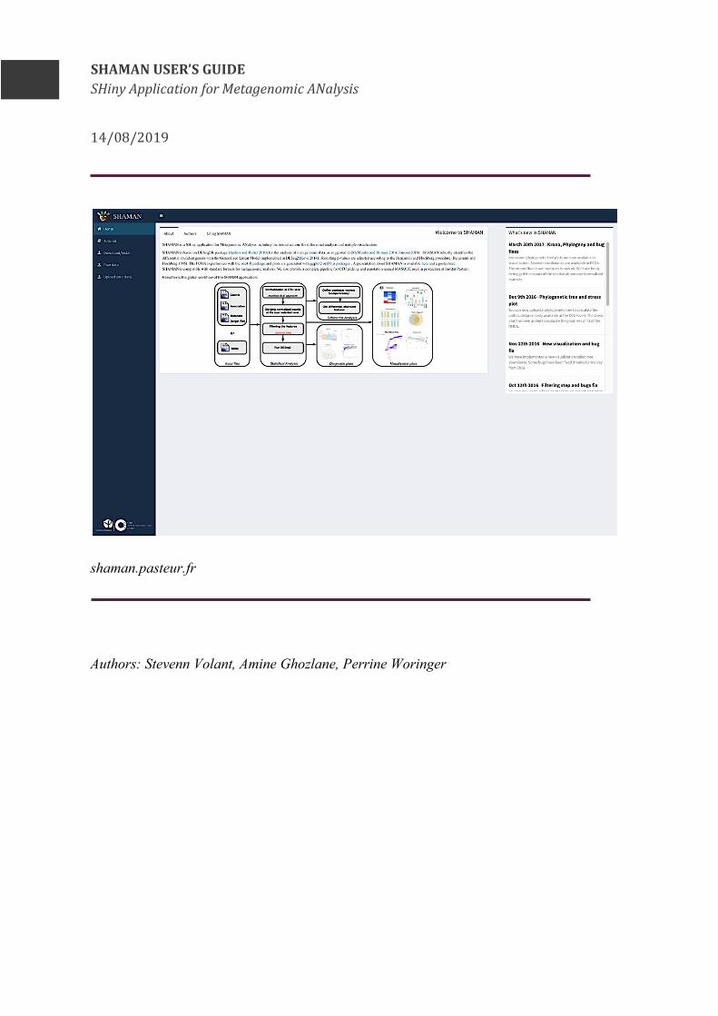
SHAMANUSER’SGUIDESHinyApplicationforMetagenomicANalysis

14/08/2019

shaman.pasteur.fr Authors: Stevenn Volant, Amine Ghozlane, Perrine Woringer

2

SUMMARY

Introduction...................................................................................................................3

Installation.....................................................................................................................4Quickinstallationinstructions.........................................................................................................................4

Tutorial............................................................................................................................7Homepage...................................................................................................................................................................7TutorialandDownload........................................................................................................................................8Rawdata......................................................................................................................................................................9Readpreparation...............................................................................................................................................9OTUprocessing.................................................................................................................................................10

Loadcountandannotationdata...................................................................................................................18

StatisticalAnalysis....................................................................................................22Buildthestatisticalmodel...............................................................................................................................22Loadingtheexperimentaldesign............................................................................................................23Definethemodel..............................................................................................................................................24

Modeloptionsandnormalization................................................................................................................26Data filtering (optional).......................................................................................................................................29Defineacontrastvector....................................................................................................................................30Assessingthestatisticalmodel......................................................................................................................31Differentialanalysis............................................................................................................................................36

Visualizations.............................................................................................................38Visualizationsoftheresults............................................................................................................................40

Overall composition........................................................................................................................................40Fold-change........................................................................................................................................................42Linksbetweenvariables...............................................................................................................................42Abundanceandtaxonomy...........................................................................................................................44

Resultcomparisons.............................................................................................................................................45Comparisonofthedifferentiallyabundantelements.....................................................................46Comparisonoffoldchange.........................................................................................................................49Comparisonofpvalue...................................................................................................................................50

Bibliography...............................................................................................................51

AppendixA..................................................................................................................52

3

INTRODUCTION

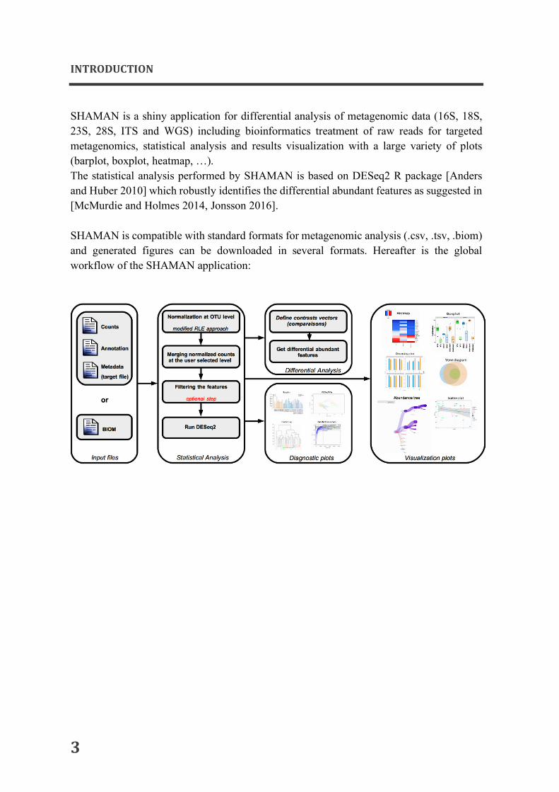
SHAMAN is a shiny application for differential analysis of metagenomic data (16S, 18S, 23S, 28S, ITS and WGS) including bioinformatics treatment of raw reads for targeted metagenomics, statistical analysis and results visualization with a large variety of plots (barplot, boxplot, heatmap, …). The statistical analysis performed by SHAMAN is based on DESeq2 R package [Anders and Huber 2010] which robustly identifies the differential abundant features as suggested in [McMurdie and Holmes 2014, Jonsson 2016]. SHAMAN is compatible with standard formats for metagenomic analysis (.csv, .tsv, .biom) and generated figures can be downloaded in several formats. Hereafter is the global workflow of the SHAMAN application:

4

INSTALLATION

Quickinstallationinstructions SHAMAN is available for local installation using Docker and R. This installation covers only the statistical analysis. The bioinformatics treatment is deported to the Institut Pasteur galaxy instance for performance reason. - Dockerinstall

Docker is the easiest way to use SHAMAN locally. It is a controlled virtual environment where every package required for SHAMAN are already installed and which have no impact on your local R installation. First, download and install Docker from https://www.docker.com/. Docker is available for Windows, Mac and Linux. Run:

Then, connect with your web browser to: http://0.0.0.0/ or http://localhost/ If port 80 is already allocated, run:

Then connect to http://0.0.0.0:3838/ or http://localhost:3838/ . You can update your local version of SHAMAN with:

- RinstallwithPackrat

SHAMAN is available for R=3.1.2. Packrat framework installation allow an easy installation of all the dependencies. Of note, raw data submission is not possible with this version. First, install R 3.1.2 as local install as follow:

#Downloadshamandockerpullaghozlane/shaman#Executeshaman,port80and5438needtobeavailabledockerrun--rm-p80:80-p5438:5438aghozlane/shaman

dockerrun--rm-p3838:80-p5438:5438aghozlane/shaman

dockerpullaghozlane/shaman

5

This installation will not interact with other R installation. Then, you can install shaman with packrat:

Now you can run SHAMAN:

- Rinstall(deprecated)

SHAMAN is available for R=3.1.2. The installation, download and execution can all be performed with a small R script:

#InstallR3.1.2wget https://pbil.univ-lyon1.fr/CRAN/src/base/R-3/R-3.1.2.tar.gz && tar -zxfR-3.1.2.tar.gzmkdir/some/location/r_bincdR-3.1.2/&&./configure--prefix=/some/location/r_bin/&&make&&makeinstall&&/some/location/r_bin/bin/R#DownloadSHAMANpackagewgetftp://shiny01.hosting.pasteur.fr/pub/shaman_package.tar.gz

#InstallSHAMANdependenciesmkdir/some/location/shaman/some/location/r_bin/bin/Rinstall.packages(c('devtools','codetools','lattice','MASS','survival','packrat'))library(devtools)devtools::install_github(c('aghozlane/nlme'))packrat::unbundle("shaman_package.tar.gz","/packrat/location/shaman")

library(packrat)packrat::init("/packrat/location/shaman")library(shiny)system("Rscript -e'library(\"shiny\");runGitHub(\"pierreLec/KronaRShy\",port=5438)'",wait=FALSE)runGitHub('aghozlane/shaman')

6

Of note, the R version has an impact on the contrast definition. For R>3.2, DESeq2 used non-expanded modeling, hence the creation of contrast vectors slightly differs and some SHAMAN features might be deactivated.

#Loadshinypackagesif(!require('shiny')){

install.packages('shiny')library(shiny)

}system("Rscript–elibrary("shiny");runGitHub("pierreLec/KronaRShy",port=5438)",wait=FALSE)#Installdependencies,downloadlastversionfromgithub,#andrunSHAMANinonecommand:runGitHub('aghozlane/shaman')

7

TUTORIAL

Homepage

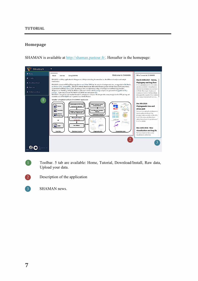
SHAMAN is available at http://shaman.pasteur.fr/. Hereafter is the homepage:

1

2 3

1 Toolbar. 5 tab are available: Home, Tutorial, Download/Install, Raw data, Upload your data. Description of the application

2

SHAMAN news.

3

8

TutorialandDownload

« Tutorial » and « Download/Install » panels are:

1 Online tutorial: it provides a description of SHAMAN usage for a set of 16S data. The dataset used is provided for download.

1

2

Installation guide. It is possible to install shaman with docker and R.

2

9

Rawdata

SHAMAN provide access to a bioinformatics workflow for analyzing targeted metagenomics data. This workflow is based on de novo clustering. Operational Taxonomic Unit (OTU) are built from reads in a given experiment and annotated by alignment against reference databases. The aim is to identify among high quality amplicon, OTU sequences that will be representative of one species and considered for annotation and quantification. The workflow can be summaries as follow:

Readpreparation

Cleaning

Cleaning step consists in the alignment of reads against the host and PhiX174 reference genome. Reads that did not align are considered for further analysis. This step is facultative but recommended. Very few amount of host DNA or Phi phage (used for calibration in every Illumina sequencing) can be identified in samples. A bowtie2 alignment with parameters (--sensitive) allows to eliminate these reads. Trimming

The trimming step consists to remove nucleotides sequences (adaptors, primers and non-confident nucleotides) in both 5’ and 3’ read ends. A list of every adaptators and primer used in Illumina, Solid, Ion torrent, Truseq, and Nextera adaptators is already

GATTACA … TTA

3031 … 161514 READ

Quality

Sequence

GATTACA … T

3031 … 16 READ trimmed Quality

Sequence

10

included in SHAMAN. But user can specify his own adaptaters. This step is performed by Alientrimmer [Criscuolo 2013]. Merging

When reads are paired, a merging step is performed using Pear [Zhang 2013]. Reads are expected to overlap a given area of the ribosomal RNA. Sequence obtained are called amplicons. OTUprocessing

The OTU clustering step is performed with Vsearch [Rognes 2016]. Dereplication

The dereplication consists in selecting one representative sequence among identical amplicon sequence. Two approaches are available: the full length and the prefix dereplication. Full length approach will group sequence that are identical for their entire length. Prefix will also group sequence of different length. Only the longest sequence will be kept. The number of identical sequences in a given sample is critical. Sequences are re-ordered by this “dereplicated abundance” which will drive the OTU clustering (see clustering section). Sequences with no identical respective are considered as singleton and are excluded of the OTU clustering process. Chimerafiltering

GATTACA … TTA Sequence

TTA … GATTACA

GATTACA … TTA

GATTACA … TTA Full length

GATTACA … TTA

GATTACA … Prefix

Biological sequence X

Biological sequence Y

Chimera formed from X and Y

11

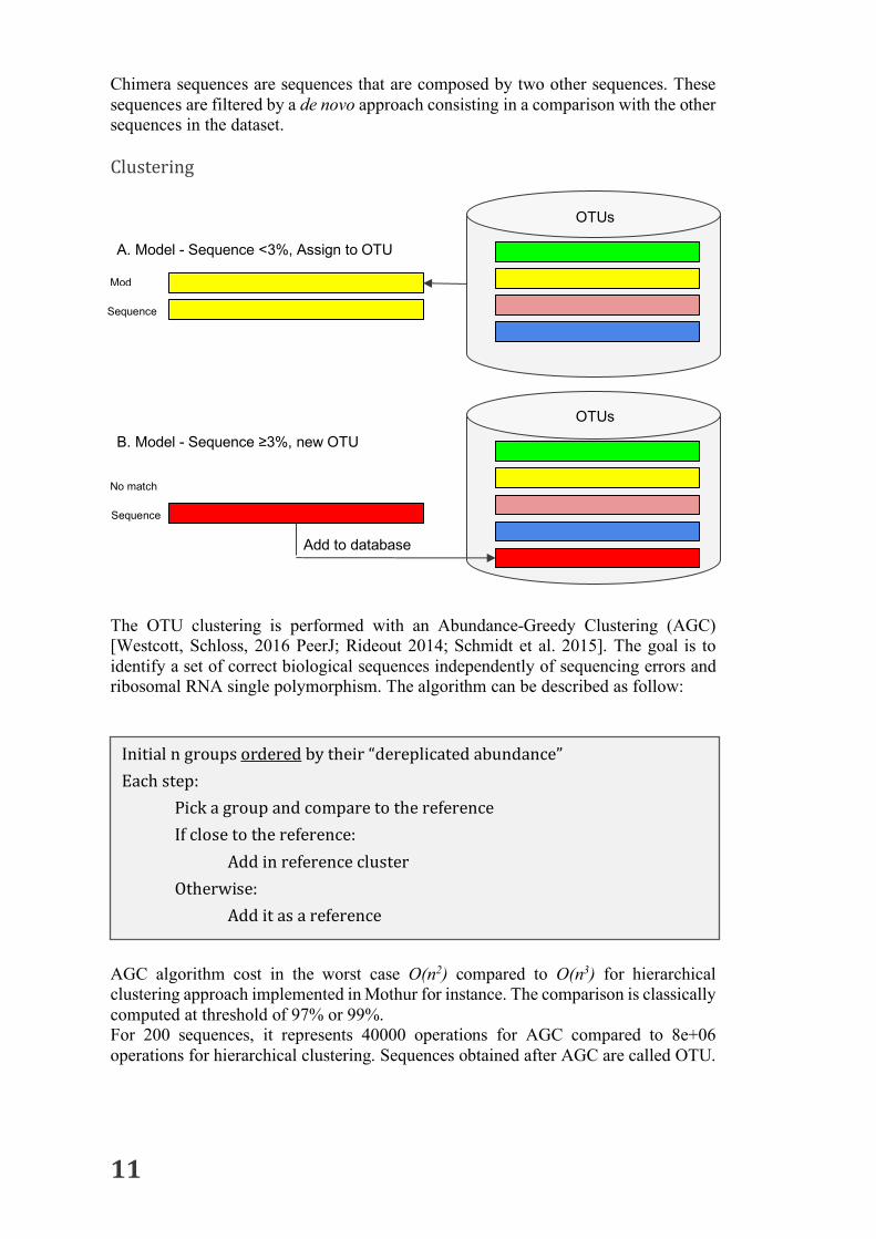
Chimera sequences are sequences that are composed by two other sequences. These sequences are filtered by a de novo approach consisting in a comparison with the other sequences in the dataset. Clustering

The OTU clustering is performed with an Abundance-Greedy Clustering (AGC) [Westcott, Schloss, 2016 PeerJ; Rideout 2014; Schmidt et al. 2015]. The goal is to identify a set of correct biological sequences independently of sequencing errors and ribosomal RNA single polymorphism. The algorithm can be described as follow:

AGC algorithm cost in the worst case O(n2) compared to O(n3) for hierarchical clustering approach implemented in Mothur for instance. The comparison is classically computed at threshold of 97% or 99%. For 200 sequences, it represents 40000 operations for AGC compared to 8e+06 operations for hierarchical clustering. Sequences obtained after AGC are called OTU.

Initialngroupsorderedbytheir“dereplicatedabundance”Eachstep:

PickagroupandcomparetothereferenceIfclosetothereference:

AddinreferenceclusterOtherwise:

Additasareference

OTUs

Mod

Sequence

A. Model - Sequence <3%, Assign to OTU

B. Model - Sequence ≥3%, new OTU OTUs

No match

Sequence

Add to database

12

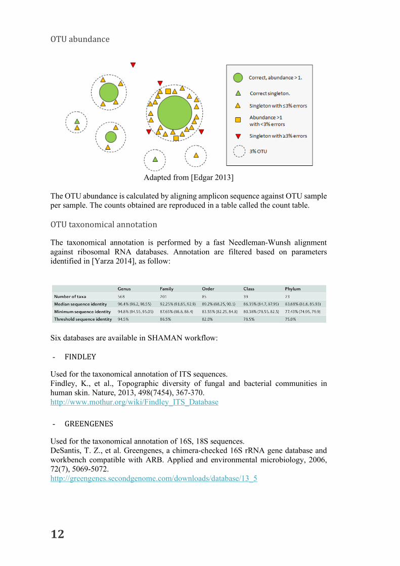
OTUabundance

Adapted from [Edgar 2013]

The OTU abundance is calculated by aligning amplicon sequence against OTU sample per sample. The counts obtained are reproduced in a table called the count table. OTUtaxonomicalannotation

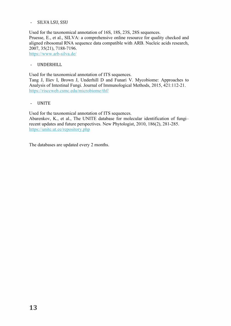
The taxonomical annotation is performed by a fast Needleman-Wunsh alignment against ribosomal RNA databases. Annotation are filtered based on parameters identified in [Yarza 2014], as follow:

Six databases are available in SHAMAN workflow: - FINDLEY

Used for the taxonomical annotation of ITS sequences. Findley, K., et al., Topographic diversity of fungal and bacterial communities in human skin. Nature, 2013, 498(7454), 367-370. http://www.mothur.org/wiki/Findley_ITS_Database

- GREENGENES

Used for the taxonomical annotation of 16S, 18S sequences. DeSantis, T. Z., et al. Greengenes, a chimera-checked 16S rRNA gene database and workbench compatible with ARB. Applied and environmental microbiology, 2006, 72(7), 5069-5072. http://greengenes.secondgenome.com/downloads/database/13_5

13

- SILVALSU,SSU

Used for the taxonomical annotation of 16S, 18S, 23S, 28S sequences. Pruesse, E., et al., SILVA: a comprehensive online resource for quality checked and aligned ribosomal RNA sequence data compatible with ARB. Nucleic acids research, 2007, 35(21), 7188-7196. https://www.arb-silva.de/ - UNDERHILL

Used for the taxonomical annotation of ITS sequences. Tang J, Iliev I, Brown J, Underhill D and Funari V. Mycobiome: Approaches to Analysis of Intestinal Fungi. Journal of Immunological Methods, 2015, 421:112-21. https://risccweb.csmc.edu/microbiome/thf/

- UNITE

Used for the taxonomical annotation of ITS sequences. Abarenkov, K., et al., The UNITE database for molecular identification of fungi–recent updates and future perspectives. New Phytologist, 2010, 186(2), 281-285. https://unite.ut.ee/repository.php

The databases are updated every 2 months.

14

This workflow is available in “Raw data” section, is installed on galaxy.pasteur.fr and makes profit on the Institut Pasteur cluster to run calculation. The usage of this workflow was simplified in this section.

4 2

1

3

Main panel allows to describe data characteristics: - type of sequencing (16S, 18S, 23S, 28S, ITS) - Paired/single end sequencing - Host of the microbiome - Specify primers - And workflow parameters

The user need to specify a mail and click on “get a key”. This key is the project identifier. It allows to follow calculation progress, view and download results.

1

Loading area for .fq, .fq.gz, .fastq and fastq.gz files 2

For paired end sequencing, files corresponding to R1 and R2 of a given sample need be paired. A pattern is required to identify R1 and R2 files. The exclusion of this pattern must allow to get the same sample name. Matched sample will be located next to its pair

3

4 Summary of the analysis.

15

For the example, we will load the mock sequencing performed with an Illumina MiSeq sequencer at Institut Pasteur using microbial community DNA from Zymobiomics (https://www.zymoresearch.com/media/amasty/amfile/attach/_D4300T_D4300_D4304_ZymoBIOMICS_DNA_Miniprep_Kit_1_1_2_LKN-SW_.pdf).

More options are available to specify primer used for sequencing and change workflow parameters when checking correspond boxes.

Primer sequences indicated in the following panels will be considered for read trimming.

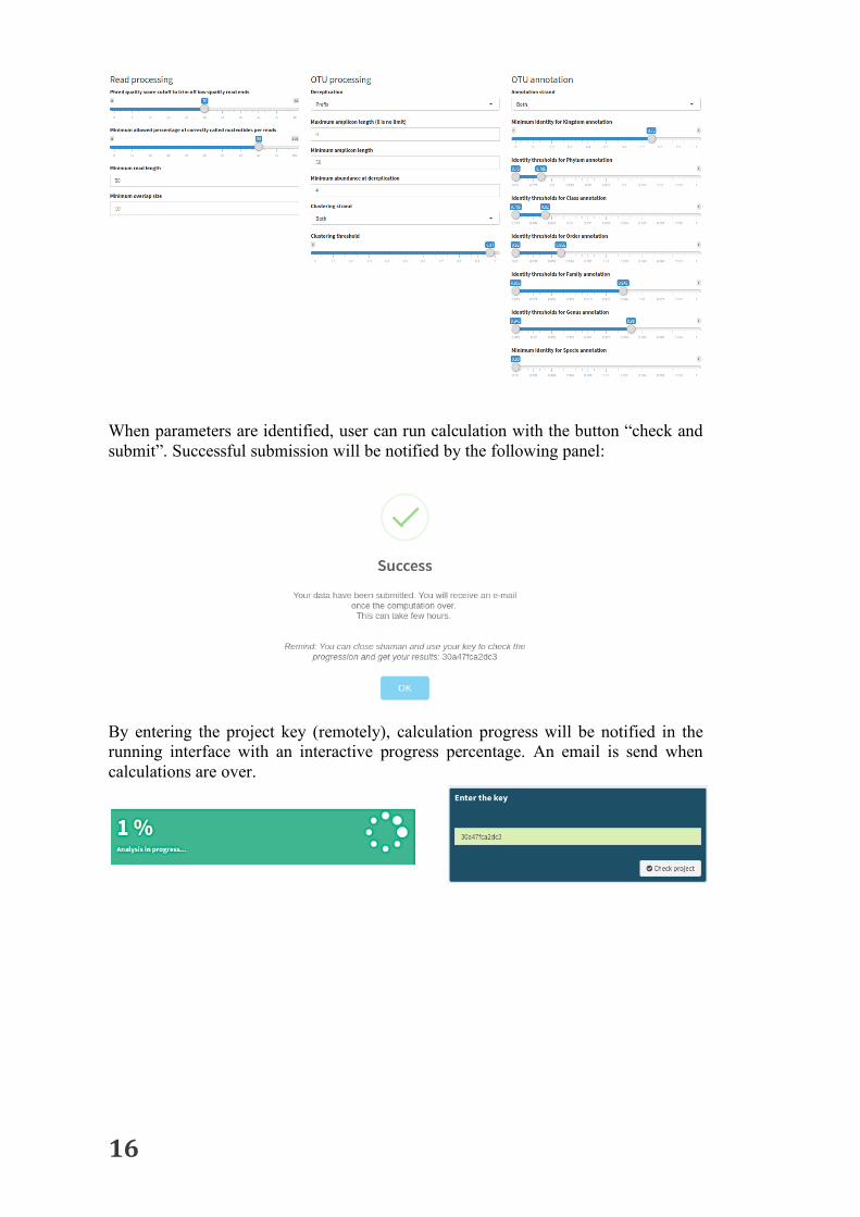
Users can also change workflow parameters for read processing, OTU processing and OTU annotation with the following panel:

1

2

2

1 When fastq files were successfully loaded, all panel turn green. The key 30a47fca2dc3 is now specific to my project.

Matched paired-end reads appears in the same order.

16

When parameters are identified, user can run calculation with the button “check and submit”. Successful submission will be notified by the following panel:

By entering the project key (remotely), calculation progress will be notified in the running interface with an interactive progress percentage. An email is send when calculations are over.

17

When calculations are terminated, an interface is available to check

A command line version of the workflow is available at https://github.com/aghozlane/masque.

1 Information about the number of sequences obtained at each clustering step and annotated against ribosomal RNA databases. Information about the read and OTU processing sample by sample 2

Panel allowing to load resulting data for corresponding databases. 3

4 Download all results.

1 2

3

4

18

Loadcountandannotationdata

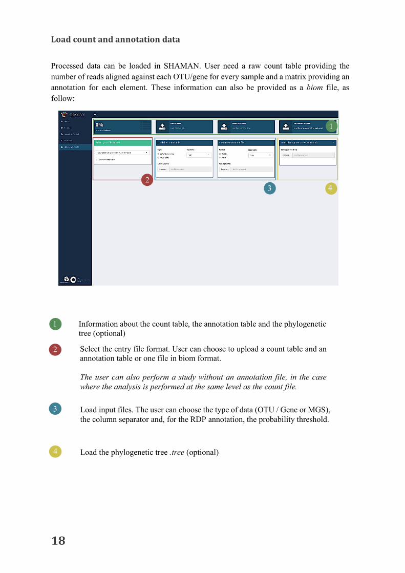
Processed data can be loaded in SHAMAN. User need a raw count table providing the number of reads aligned against each OTU/gene for every sample and a matrix providing an annotation for each element. These information can also be provided as a biom file, as follow:

1

3 4 2

1 Information about the count table, the annotation table and the phylogenetic tree (optional) Select the entry file format. User can choose to upload a count table and an annotation table or one file in biom format. The user can also perform a study without an annotation file, in the case where the analysis is performed at the same level as the count file.

2

Load input files. The user can choose the type of data (OTU / Gene or MGS), the column separator and, for the RDP annotation, the probability threshold.

3

4 Load the phylogenetic tree .tree (optional)

4

19

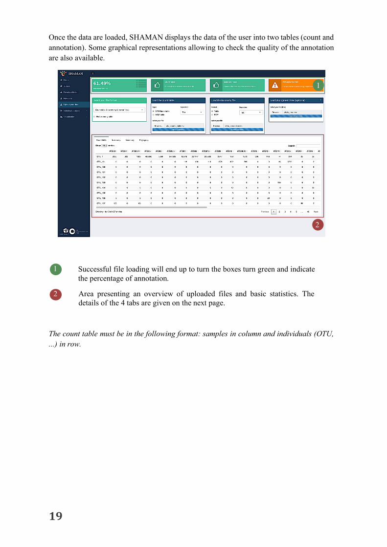
Once the data are loaded, SHAMAN displays the data of the user into two tables (count and annotation). Some graphical representations allowing to check the quality of the annotation are also available.

The count table must be in the following format: samples in column and individuals (OTU, ...) in row.

1

2

1 Successful file loading will end up to turn the boxes turn green and indicate the percentage of annotation.

Area presenting an overview of uploaded files and basic statistics. The details of the 4 tabs are given on the next page.

2

20

The 4 tabs of the previous box are the following

1 Count table with sample in column and OTU/genes in row.

Annotation table with different annotation levels in column and the OTU/genes in row.

2

Figure presenting the percentage of OTU/genes annotated at each annotation level and the number of samples at each level.

3

4 Figure of the phylogenetic tree (only if a phylogenetic .tree is loaded, optional)

21

Once the data has been loaded, two new tabs appear "Statistical analysis" and "Visualization". Statistical analysis - This tab is divided into 3 sub-tabs:

• Run differential analysis: allows to define the statistical model as well as some options, the taxonomic level and to create the vectors of contrasts for defining comparisons

• Diagnostic plots: many different visualizations (barplots, boxplots, clustering, PCA, PCoA, NMDS, ...) are available to control the design of the experiment, check the normalization and identify possible sequencing problems.

• Tables: get the results of the differential analysis for each defined contrast vector.

Visualization - This tab is divided into 2 sub-tabs: • Global views: provides many interactive representations (barplots, heatmap,

boxplots, krona, tree of abundance, network plot, curves of rarefaction, diversities) to visualize sample composition as well as the results of the differential analysis according to the experimental design.

• Plots comparison: several plots (venn diagram, heatmap of the log2-foldchange, p-value density, UpSet plot) are provided to compare the results of the analysis for each contrast (at least 2 contrast vectors have to be defined)

22

STATISTICALANALYSIS

SHAMAN statistics are based on DESeq2 package. This package requires the definition of a statistical model and to set up several parameters (not presented here). The different steps can be summarized as follow:

1. Data normalization (calculation of size factors) 2. Estimation of the dispersion based on a modeling of the average normalized counts

and the empirical dispersion. 3. Adjustment of the generalized linear model based on the negative binomial

distribution and a log link function. 4. Statistical test (Wald test) performed on model parameters 5. Outlier filtering 6. Correction of the multiple tests

DESeq2 has been shown as one of the best methods to identify differentially abundant features. Buildthestatisticalmodel

In order to build the statistical model, the user must first provide the experimental design (target file) and select the taxonomic level. It is then necessary to select the variables of interest describing the biological phenomenon studied as well as the possible interactions between these variables. Before starting the analysis, the user can set the various options related to DESeq2 such as the independent filtering, the shape of the dispersion modeling, the method of correction of the multiple tests ... (for more information see [ Love et al., 2014]). All these steps must be carried out in the "Run differential analysis" sub-tab.

23

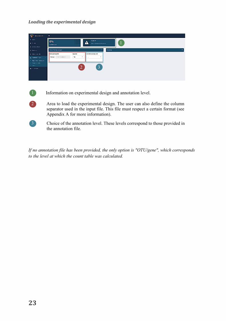
Loadingtheexperimentaldesign

If no annotation file has been provided, the only option is "OTU/gene", which corresponds to the level at which the count table was calculated.

2 3

1

1 Information on experimental design and annotation level. Area to load the experimental design. The user can also define the column separator used in the input file. This file must respect a certain format (see Appendix A for more information).

2

Choice of the annotation level. These levels correspond to those provided in the annotation file.

3

24

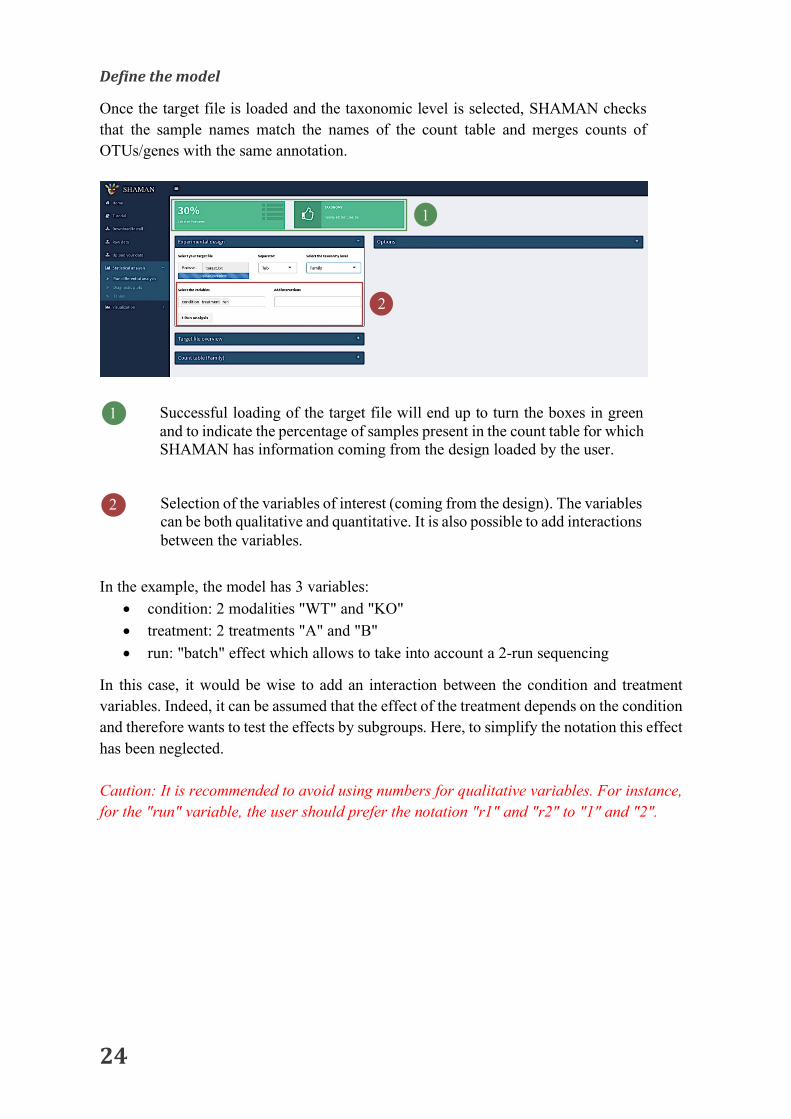
Definethemodel

Once the target file is loaded and the taxonomic level is selected, SHAMAN checks that the sample names match the names of the count table and merges counts of OTUs/genes with the same annotation.

In the example, the model has 3 variables:

• condition: 2 modalities "WT" and "KO"• treatment: 2 treatments "A" and "B"• run: "batch" effect which allows to take into account a 2-run sequencing

In this case, it would be wise to add an interaction between the condition and treatment variables. Indeed, it can be assumed that the effect of the treatment depends on the condition and therefore wants to test the effects by subgroups. Here, to simplify the notation this effect has been neglected. Caution: It is recommended to avoid using numbers for qualitative variables. For instance, for the "run" variable, the user should prefer the notation "r1" and "r2" to "1" and "2".

2

1

1 Successful loading of the target file will end up to turn the boxes in green and to indicate the percentage of samples present in the count table for which SHAMAN has information coming from the design loaded by the user.

Selection of the variables of interest (coming from the design). The variables can be both qualitative and quantitative. It is also possible to add interactions between the variables.

2

25

1 Overview of the target file loaded by the user. This file describes each sample by one or more variables (qualitative and/or quantitative). The user can remove some samples of poor quality and export the new target file. Overview of the "aggregated" normalized count table at the taxonomic level selected by the user. The user can export the table of normalized counts and/or relative abundances

2

2 1

26

Modeloptionsandnormalization

• Type of transformation

Two transformations are available in DESeq2, VST (Variance Stabilizing Transformation) and rlog (regularized log transformation). The data being heteroscedastic, this transformation makes it possible to eliminate the dependence of the variance on the mean. It is only used to visualize and/or classify the data (modeling is done on the counts). When the number of samples is large, it is recommended to use VST transformation which is faster than the rlog.

• Independent filtering This filter based on the average counts over all the samples. It aims at filtering the individuals (species, genera, ...) which are very unlikely to be differentially abundant. The threshold used for the filter is determined such that the number of significant individuals reach its maximum for a given FDR.

• p-value adjustment Two usual methods for multiple correction by FDR are proposed: Benjamini-Hochberg et Benjamini-Yekuteli.

• Level of significance Level of significance for the statistical test. By default, this value is 5%.

• Cooks cut-off The log-fold change value is strongly influenced by outliers. To detect outliers, the Cooks distance which measure the impact of removing a sample on the estimation of the parameters can be used. The 99th percentile of the Fisher distribution (F (p, m-p), with p the number of parameters and m the number of samples) is used as a threshold for the Cooks distance.

27

• Local function

To calculate the size factors (used to normalize the data), there are two options "median" or "shorth". The first one, "median" is the default method which aims at calculating the median of the ratio between counts and the geometric mean (see normalization section for more details). The second one, "shorth", calculates the average of the smallest interval that covers half of the values. This option is especially recommended for low counts.

• Relationship For each feature, the dispersion is estimated by modeling the relationship between empirical dispersion and mean counts. To model this relation, three methods are proposed:

ü a parametric regression of the form

ü a local regression which makes it possible to obtain a better modeling when the form in "1/x" is not well adapted.

ü the mean. This approach can be used when the number of individuals is small.

↵tr(µ̄) = ↵0 +a1µ̄

28

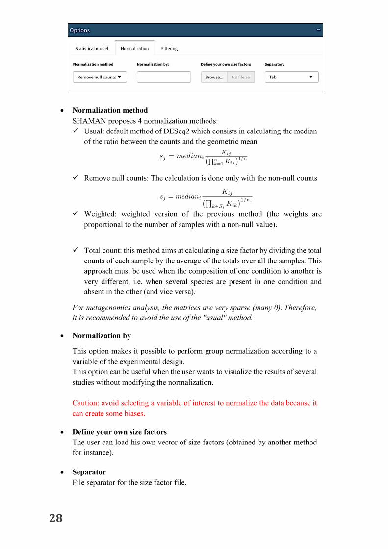
• Normalization method SHAMAN proposes 4 normalization methods: ü Usual: default method of DESeq2 which consists in calculating the median

of the ratio between the counts and the geometric mean

ü Remove null counts: The calculation is done only with the non-null counts

ü Weighted: weighted version of the previous method (the weights are

proportional to the number of samples with a non-null value).

ü Total count: this method aims at calculating a size factor by dividing the total

counts of each sample by the average of the totals over all the samples. This approach must be used when the composition of one condition to another is very different, i.e. when several species are present in one condition and absent in the other (and vice versa).

For metagenomics analysis, the matrices are very sparse (many 0). Therefore, it is recommended to avoid the use of the "usual" method.

• Normalization by

This option makes it possible to perform group normalization according to a variable of the experimental design. This option can be useful when the user wants to visualize the results of several studies without modifying the normalization. Caution: avoid selecting a variable of interest to normalize the data because it can create some biases.

• Define your own size factors The user can load his own vector of size factors (obtained by another method for instance).

• Separator

File separator for the size factor file.

sj = medianiKij

(Qn

k=1 Kik)1/n

sj = medianiKij

�Qk2Si

Kik

�1/ni

29

Data filtering (optional)

In some cases, when many elements have low counts and/or are only detected for a small number of samples, it may be useful to filter them before starting the analysis. This will not have a strong influence on the results of the differential analysis. Indeed, the independent filtering already filter these elements. For studies with many features, it allows to reduce the computation time.

1 2

3

1 Threshold on the occurrence in all samples. By default, the threshold set by SHAMAN corresponds to 20% of the samples.

Threshold on average abundance. To calculate a threshold automatically, SHAMAN performs a linear regression between the number of sample with an average abundance of at least x and the average abundance.

2

Figure representing the number of occurrences in all samples compared to the average abundance. The red dots correspond to the elements that will be filtered out once the two filters are applied.

3

30

Defineacontrastvector

Once the statistical analysis is done, SHAMAN provides the list of parameters corresponding to the variables included in the model. From the estimation of these parameters, the user can test different effects. Denote by 𝛽" the vector of parameters. Let c be a vector of contrasts, define as a linear combination of parameters. We then use a Wald test whose test statistic is distributed according to a standard normal distribution: The matrix 𝛴" corresponds to the variance-covariance matrix of the model parameters. Example 1 If the user wants to test whether there is a treatment effect (A vs B), it corresponds to test whether the difference A-B is zero. To do so, a contrast vector composed of 1 and -1 for the parameters associated with the treatments A and B has to be created. The hypotheses of the test will be as follows:

$H0: 𝛽( − 𝛽* = 0H1: 𝛽( − 𝛽* ≠ 0

In a complex experimental design, many comparisons can be done by defining a set of contrast vectors. Example 2 Assume that we have an experimental design with measurements for 3 treatments A, B and C. The user wants to know if the effect of treatment C corresponds to the average of treatments A and B. In this case, 3 parameters will be estimated (one for each treatment). To get the desired comparison, the user must define the following contrast vector:

�cip

ct⌃ic⇠ N(0, 1)

�ci = ct�i

31

2

3

1 4

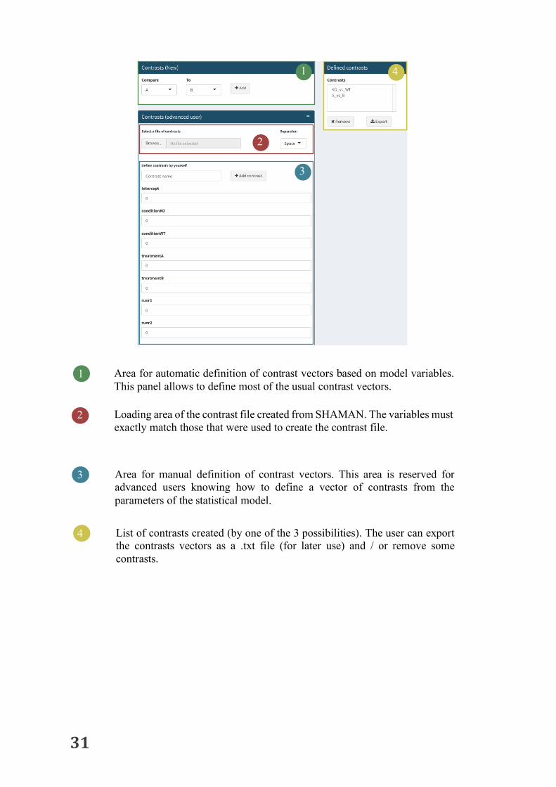
1 Area for automatic definition of contrast vectors based on model variables. This panel allows to define most of the usual contrast vectors.

Loading area of the contrast file created from SHAMAN. The variables must exactly match those that were used to create the contrast file.

2

Area for manual definition of contrast vectors. This area is reserved for advanced users knowing how to define a vector of contrasts from the parameters of the statistical model.

3

4 List of contrasts created (by one of the 3 possibilities). The user can export the contrasts vectors as a .txt file (for later use) and / or remove some contrasts.

32

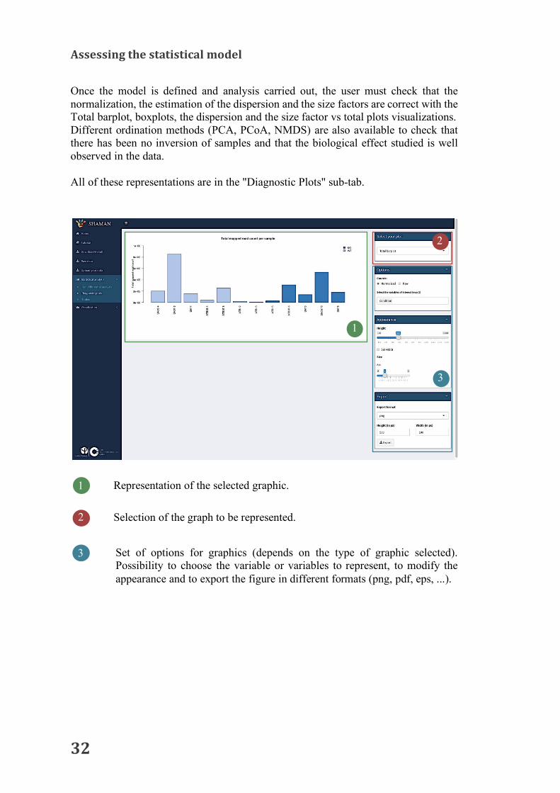
Assessingthestatisticalmodel

Once the model is defined and analysis carried out, the user must check that the normalization, the estimation of the dispersion and the size factors are correct with the Total barplot, boxplots, the dispersion and the size factor vs total plots visualizations. Different ordination methods (PCA, PCoA, NMDS) are also available to check that there has been no inversion of samples and that the biological effect studied is well observed in the data. All of these representations are in the "Diagnostic Plots" sub-tab.

2

3

1

1 Representation of the selected graphic.

Selection of the graph to be represented. 2

Set of options for graphics (depends on the type of graphic selected). Possibility to choose the variable or variables to represent, to modify the appearance and to export the figure in different formats (png, pdf, eps, ...).

3

33

Interpretation: These diagrams allow to identify possible issues linked to the sequencing depth. In the example presented, one of the "SN07-8" samples (in dashed lines) seems to have a large number of reads aligned with the others. This sample can also be detected as an outlier when looking at the representation of densities. In this context, the user must give attention to this sample and check if the whole bioinformatics process went well. It might be necessary to delete this sample from the analysis. Note: The rarefaction curves presented in the "Visualization" section can also be used to determine if one sample must be deleted from the study.

1 Barplot of the counts for each sample Barplot of the null counts for each sample 2

Barplot of the most abundant features

3

4 Density plot of the counts in log2

2

3

1

4

34

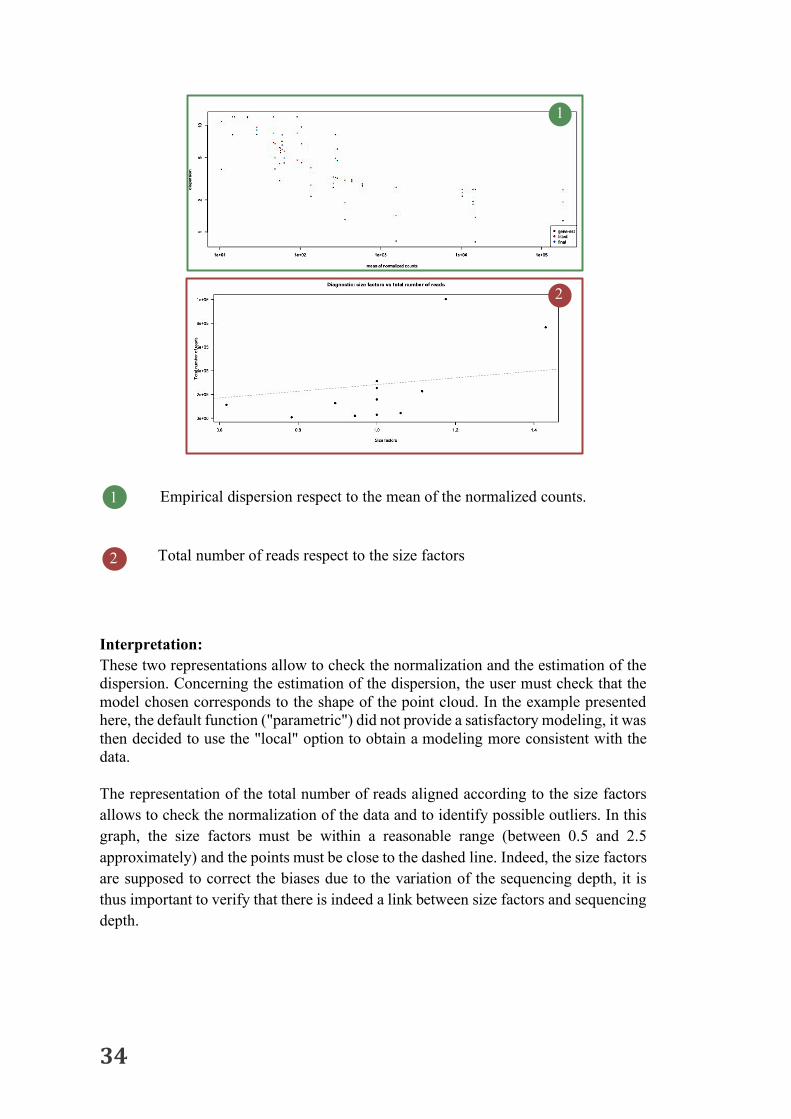
Interpretation: These two representations allow to check the normalization and the estimation of the dispersion. Concerning the estimation of the dispersion, the user must check that the model chosen corresponds to the shape of the point cloud. In the example presented here, the default function ("parametric") did not provide a satisfactory modeling, it was then decided to use the "local" option to obtain a modeling more consistent with the data. The representation of the total number of reads aligned according to the size factors allows to check the normalization of the data and to identify possible outliers. In this graph, the size factors must be within a reasonable range (between 0.5 and 2.5 approximately) and the points must be close to the dashed line. Indeed, the size factors are supposed to correct the biases due to the variation of the sequencing depth, it is thus important to verify that there is indeed a link between size factors and sequencing depth.

1 Empirical dispersion respect to the mean of the normalized counts.

Total number of reads respect to the size factors

2

2

1

35

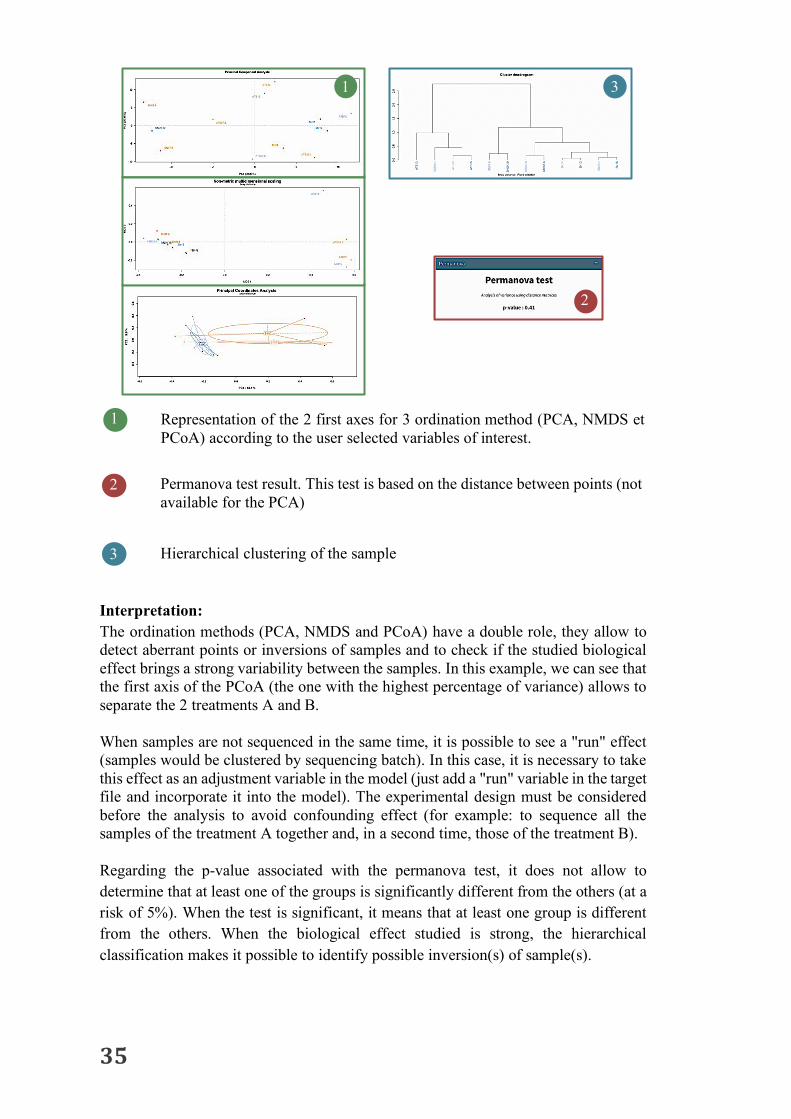
Interpretation: The ordination methods (PCA, NMDS and PCoA) have a double role, they allow to detect aberrant points or inversions of samples and to check if the studied biological effect brings a strong variability between the samples. In this example, we can see that the first axis of the PCoA (the one with the highest percentage of variance) allows to separate the 2 treatments A and B. When samples are not sequenced in the same time, it is possible to see a "run" effect (samples would be clustered by sequencing batch). In this case, it is necessary to take this effect as an adjustment variable in the model (just add a "run" variable in the target file and incorporate it into the model). The experimental design must be considered before the analysis to avoid confounding effect (for example: to sequence all the samples of the treatment A together and, in a second time, those of the treatment B). Regarding the p-value associated with the permanova test, it does not allow to determine that at least one of the groups is significantly different from the others (at a risk of 5%). When the test is significant, it means that at least one group is different from the others. When the biological effect studied is strong, the hierarchical classification makes it possible to identify possible inversion(s) of sample(s).

2

3 1

1 Representation of the 2 first axes for 3 ordination method (PCA, NMDS et PCoA) according to the user selected variables of interest.

Permanova test result. This test is based on the distance between points (not available for the PCA)

2

Hierarchical clustering of the sample

3

36

Differentialanalysis

Once the analysis is done, the results are available in tabular form in the "Table" tab.

1

3 2

4

5

6 7

8

1 4 tables are available: ü Significant: list of elements detected as differentially abundant ü Complete: list with all elements ü Up, down: lists of the elements detected as differentially abundant

according to the sign of the log2 fold-change

Result table: ü baseMean: Average of normalized counts on all the samples ü FoldChange: Estimated fold change for selected contrast ü Log2FoldChange: Fold change transformed in log2 ü Pvalue_adjusted: adjusted p-value (by default p-values are adjusted by

BH procedure, other methods are available)

2

2 plots are available: ü Bar chart: log2 Fold Change for each element ü Volcano plot: p value versus fold change (scatterplot)

3

Area to display the plot 4

Selection of the desired comparison based on the user defined contrast vectors. 5

Reorder data: this will affect both the result tables and the bar chart. 6

List of the options to modify the appearance of the plot (depends on the selected plot)

7

Export results: ü For tables, the user can choose the table to export as well as the

column separator. ü For plots, the user can select the format (png, svg, eps, pdf) as well

as the size of the figure to be exported.

8

37

Interpretation: The tables presented above allows to quickly identify the elements that have a significant change in term of abundance between the conditions studied. The presented p-values correspond to the p-values of the Wald test (after correction for multiple comparisons) at the threshold of significance chosen (e.g. 5%). BaseMean informs about the mean abundance element (species, gender, ...). Note: the log2FoldChange are obtained from the parameter estimates and then the values are shrunk toward 0 for features with a high variance (strongly impacts the low counts). The bar chart and the volcano plot enable to view at a glance the data contained in the last two columns of the table (log2FoldChange and p value).

Bar chart

Volcano plot

Their appearance can be customized by the user in the “Plot options” box. Those settings (except the dimensions) will be kept if the plot is exported. The color settings are shared by the plots, and the colors can be chosen either by selecting one in the color picker, or by typing a valid color name or hexadecimal color code. For volcano plot, the threshold used for Y-axis is deduced from the significance threshold chosen for the differential analysis. The user can also define a threshold for X-axis, this will however affect only the volcano plot.

38

VISUALIZATIONS

SHAMAN offers both a robust statistical analysis of data and a wide range of representations (barplots, heatmap, boxplots, abundance tree, scatterplot, diversity, rarefaction curves, krona and Venn diagrams) allowing a complete analysis of the results. They are divided into two categories:

ü Globalviews:plotsallowing tovisualize featureabundance according to thevariablesdefinedinthetargetfile.

ü Comparisonplots:specificvisualizationtocompareresultsobtainedfor2ormorecontrast.

Regardless of the type of visualization used, SHAMAN offers many options to the user (which will remain active from one representation to another). These options are in a column to the right of the visualizations and consists of 4 elements.

39

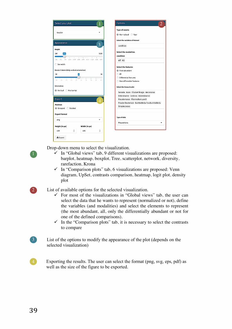
1 Drop-down menu to select the visualization.

ü In “Global views” tab, 9 different visualizations are proposed: barplot, heatmap, boxplot, Tree, scatterplot, network, diversity, rarefaction, Krona

ü In “Comparison plots” tab, 6 visualizations are proposed: Venn diagram, UpSet, contrasts comparison, heatmap, logit plot, density plot

List of available options for the selected visualization. ü For most of the visualizations in “Global views” tab, the user can

select the data that he wants to represent (normalized or not), define the variables (and modalities) and select the elements to represent (the most abundant, all, only the differentially abundant or not for one of the defined comparisons).

ü In the “Comparison plots” tab, it is necessary to select the contrasts to compare

2

List of the options to modify the appearance of the plot (depends on the selected visualization)

3

4 Exporting the results. The user can select the format (png, svg, eps, pdf) as well as the size of the figure to be exported.

2

3

1

4

40

Visualizationsoftheresults In the "Global views" tab, nine interactive visualizations are available to view the results. Note: The interpretation of targeted metagenomics data must be done carefully. rRNA are present in several copy number in bacterial genomes [Vetrovsky and Baldrian 2013, Klappenbach 2001] from 1 to 15. In consequence, it is possible to analyze the abundance of one given genus between conditions but not to compare the abundance of two genera. Overall composition

Barplot or heatmap are ideal visualizations for the analysis of the whole study. These representations make it possible to quickly visualize the differences between the conditions studied.

Interpretation: The two previous figures show that the overall composition varies between the treatments (A and B) but not for the conditions (KO and WT) on the 12 most abundant. This observation is reinforced by the hierarchical clustering in the heatmap that groups the treatments between them. The rarefaction curves and the diversity measures also provide an overview of the global composition according to the metadata.

1 Barplot of the 12 most abundant elements. Each color represents the proportion of each element. Heatmap for the 12 most abundant items per variable. The color depends on the average level of abundance. Dark red = very abundant; Dark blue = low abundance.

2

2 1

41

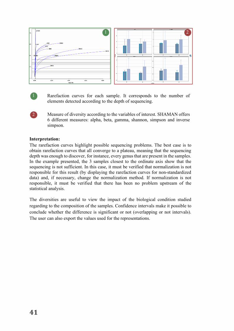
Interpretation: The rarefaction curves highlight possible sequencing problems. The best case is to obtain rarefaction curves that all converge to a plateau, meaning that the sequencing depth was enough to discover, for instance, every genus that are present in the samples. In the example presented, the 3 samples closest to the ordinate axis show that the sequencing is not sufficient. In this case, it must be verified that normalization is not responsible for this result (by displaying the rarefaction curves for non-standardized data) and, if necessary, change the normalization method. If normalization is not responsible, it must be verified that there has been no problem upstream of the statistical analysis. The diversities are useful to view the impact of the biological condition studied regarding to the composition of the samples. Confidence intervals make it possible to conclude whether the difference is significant or not (overlapping or not intervals). The user can also export the values used for the representations.

2 1

1 Rarefaction curves for each sample. It corresponds to the number of elements detected according to the depth of sequencing. Measure of diversity according to the variables of interest. SHAMAN offers 6 different measures: alpha, beta, gamma, shannon, simpson and inverse simpson.

2

42

Fold-change

Boxplots are the usual representation to visualize the results of the differential analysis and log2 fold-change estimated. For each selected element, SHAMAN represents a boxplot for all the modalities of the variables of interest (with a different color). This representation highlights the differences identified during the differential analysis. For example, for the family Enterobacteriaceae (top right), it is clear that treatment B reduces the abundance of this family (whatever the condition). This effect was detected as significant in the result tables (3rd row of the table). Linksbetweenvariables

SHAMAN enables to cross abundance levels between two elements and to measure their correlation. It is also possible to model the abundance of a specie with respect to diversity or to an auxiliary variable like age, bmi, ... which can be informative especially for clinical dataset. To realize these different crossings, SHAMAN proposes a scatterplot allowing to represent all the couples of elements, to change the points (form and color) according to the variables of interest and to add a third variable on which depends the size of the points.

43

Theusercanalsoaddalinearregression(blueline)withconfidencearea(grayarea).Theequationoftheline,thecoefficientofdeterminationR2andthetestsfor slope and intercept are then available. The user can also access to thecorrelationtable(PearsonorSpearman).Furthermore, it ispossible tovisualize the correlationbetween the respectiveabundanceofallelementatoncethanksto thenetworkplot.Eachelement isrepresentedbyanodelinkedtoeveryotherelementtowhichheissignificantlycorrelated(thecoloroftheedgedependingonthesignofthecorrelation).

44

Forthisplot,correlationsarecomputedusingPearson’smethod,andthepvaluesareadjustedformultiplecomparisonsusingHolm’smethod.Theusercanselectanauxiliaryvariableandthenodeswillbecoloredaccordingtocorrelationbetweenabundanceineachsampleandtheselectedvariable.Ifthechosenvariableisnotquantitative,itisnecessarytoselectthevaluestoconsideras“1”,amongallthepossiblevaluesofthequalitativevariable.Othervalueswillbesetto“0”.Thisplotcanbeexportedas.html.Thiswillpreserveinteractivity(movingnodes,showinglabelswhenhovering).Abundanceandtaxonomy

Allpreviousrepresentationsallowtovisualizetheresultsoftheanalysisattheleveldefinedbytheuserduringthedefinitionofthestatisticalmodel.Thetwofollowingfiguresgiveadifferentperspective.

2 1

1 Abundance tree according to the taxonomic level. The user can choose the samples they wish to represent. Representation in the form of a krona plot1. This interactive visualization allows to navigate through different taxonomic levels.

2

1https://github.com/marbl/Krona/wiki

45

Resultcomparisons

The main objective of SHAMAN is to perform a quantitative study of the differences between experimental conditions. A more qualitative approach is proposed in SHAMAN to compare the results of different studies. This is available through 6 representations in the “Comparison plots” tab:

ü Venn diagram ü UpSet ü Contrasts comparison ü Heatmap ü Logit plot ü Density plot

This type of representation allows to compare the results of several studies from a qualitative point of view. In many cases, a quantitative analysis can also be performed (with 2 comparisons) by defining a suitable contrast ("advanced user" mode).

46

Comparisonofthedifferentiallyabundantelements

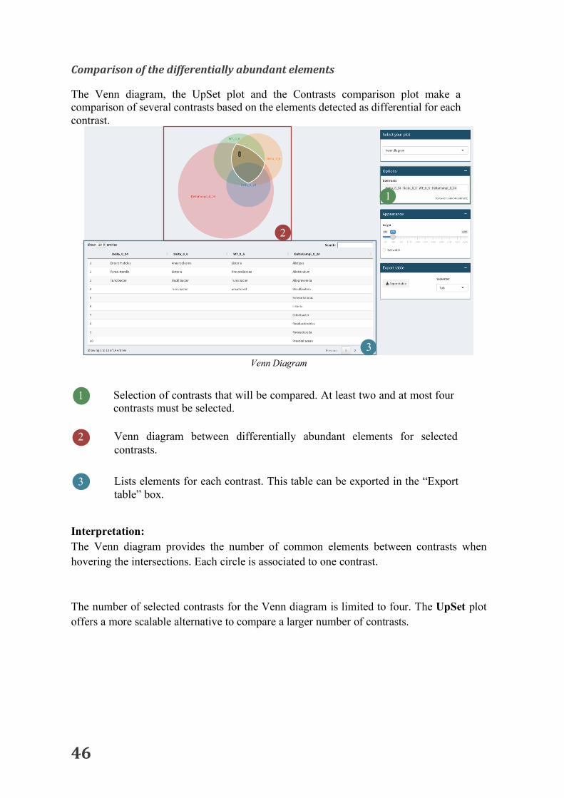
The Venn diagram, the UpSet plot and the Contrasts comparison plot make a comparison of several contrasts based on the elements detected as differential for each contrast.

Venn Diagram

Interpretation: The Venn diagram provides the number of common elements between contrasts when hovering the intersections. Each circle is associated to one contrast. The number of selected contrasts for the Venn diagram is limited to four. The UpSet plot offers a more scalable alternative to compare a larger number of contrasts.

1 Selection of contrasts that will be compared. At least two and at most four contrasts must be selected. Venn diagram between differentially abundant elements for selected contrasts.

2

Lists elements for each contrast. This table can be exported in the “Export table” box.

3

2

3

1

47

UpSet

1 Selection of contrasts that will be compared. At least two and at most four contrasts must be selected. UpSet plot: Each bar represents the number of elements that are differential for all the contrasts marked with a dot below, and are not differential for any other contrasts.

2

Table: lists the elements in each intersection. 3

To export the plot or the table

4

2

4

1

3

48

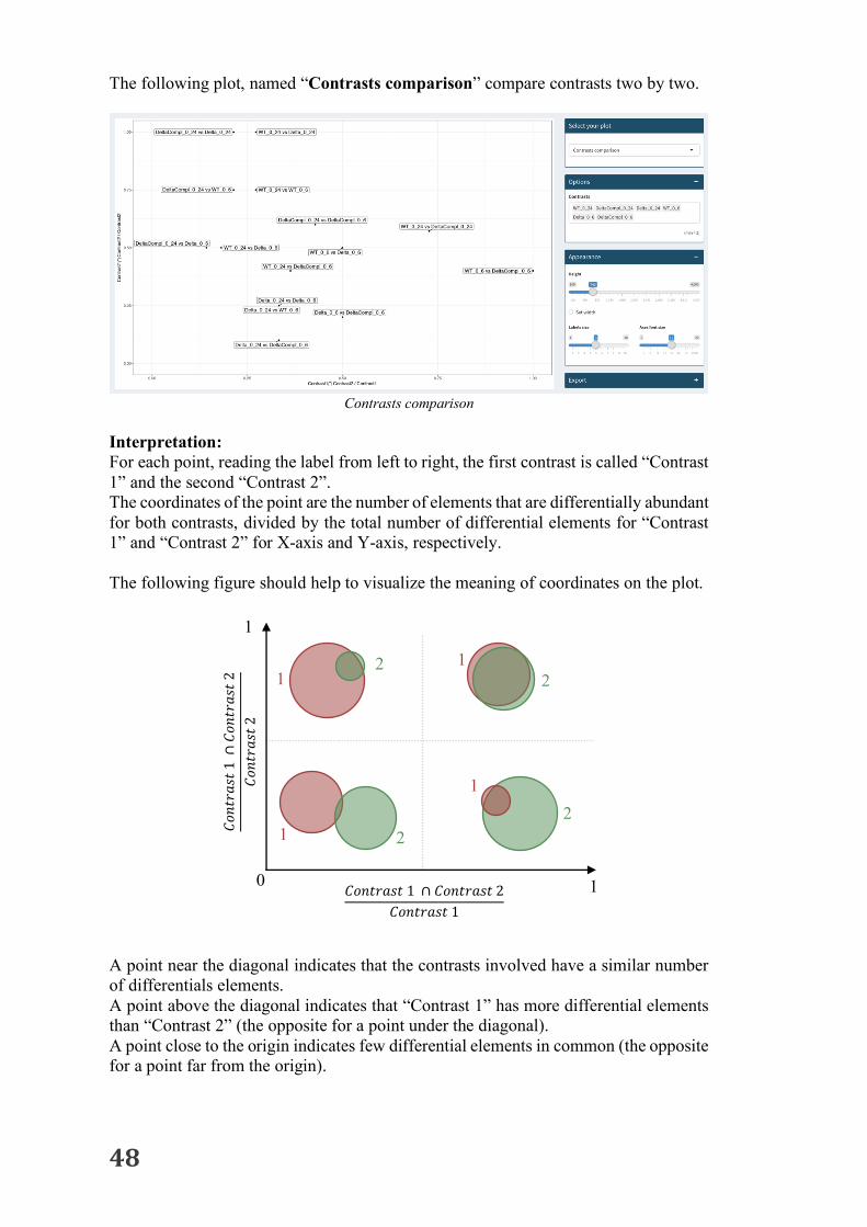
The following plot, named “Contrasts comparison” compare contrasts two by two.

Contrasts comparison

Interpretation: For each point, reading the label from left to right, the first contrast is called “Contrast 1” and the second “Contrast 2”. The coordinates of the point are the number of elements that are differentially abundant for both contrasts, divided by the total number of differential elements for “Contrast 1” and “Contrast 2” for X-axis and Y-axis, respectively. The following figure should help to visualize the meaning of coordinates on the plot. A point near the diagonal indicates that the contrasts involved have a similar number of differentials elements. A point above the diagonal indicates that “Contrast 1” has more differential elements than “Contrast 2” (the opposite for a point under the diagonal). A point close to the origin indicates few differential elements in common (the opposite for a point far from the origin).

𝐶𝑜𝑛𝑡𝑟𝑎𝑠𝑡1∩

𝐶𝑜𝑛𝑡𝑟𝑎𝑠𝑡2

𝐶𝑜𝑛𝑡𝑟𝑎𝑠𝑡2

𝐶𝑜𝑛𝑡𝑟𝑎𝑠𝑡1 ∩ 𝐶𝑜𝑛𝑡𝑟𝑎𝑠𝑡2𝐶𝑜𝑛𝑡𝑟𝑎𝑠𝑡1

2 2

2 2

1

1

1

1

0

1

1

49

Comparisonoffoldchange

The heatmap of the log2 fold change illustrates the strength of the difference between several contrasts.

Interpretation: This representation allows to identify common elements between 2 or more contrasts. The shade of color gives the direction and the strength of the difference.

1 List of the different options proposed to draw the heatmap.

Representation of log2 fold changes as a heatmap. The color depends on the value of the log2 fold change. Dark red: high positive value; Dark blue: high negative value; White: null value.

2

2

1

50

Comparisonofpvalue

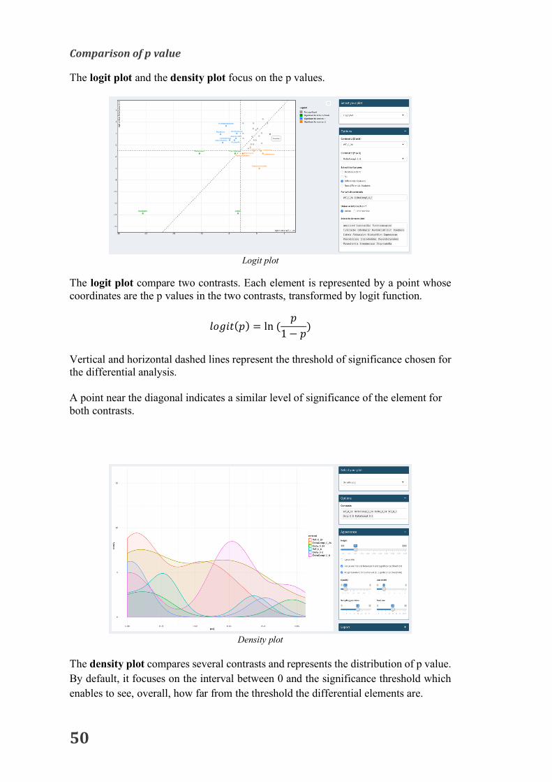
The logit plot and the density plot focus on the p values.

Logit plot

The logit plot compare two contrasts. Each element is represented by a point whose coordinates are the p values in the two contrasts, transformed by logit function.

𝑙𝑜𝑔𝑖𝑡(𝑝) = ln(𝑝

1 − 𝑝)

Vertical and horizontal dashed lines represent the threshold of significance chosen for the differential analysis. A point near the diagonal indicates a similar level of significance of the element for both contrasts.

Density plot

The density plot compares several contrasts and represents the distribution of p value. By default, it focuses on the interval between 0 and the significance threshold which enables to see, overall, how far from the threshold the differential elements are.

51

BIBLIOGRAPHY

AndersandHuber,Differentialexpressionanalysisforsequencecountdata,GenomeBiology,2010Jonsson V, Österlund T, Nerman O et al. Statistical evaluation of methods foridentification of differentially abundant genes in comparative metagenomics. BMCGenomics2016;17:78Love,HuberandAnders,ModeratedestimationoffoldchangeanddispersionforRNA-SeqdatawithDESeq2,GenomeBiology,2014McMurdie,P.J.&Holmes,S.Wastenot,wantnot:whyrarefyingmicrobiomedataisinadmissible.PLOSComput.Biol.10,e1003531(2014)

52

APPENDIXA

How to create a target file for Shaman

format, contents and constraints

The target file is required for each analysis done with Shaman. It must contain all the available information on the samples (corresponding to the metadata) that will be used to build the statistical model and/or to visualize the data. To be loaded in Shaman the target file must respect some properties

1. The first column is dedicated to the sample name which mustcorrespondexactlytothecolumnnamesofthecountmatrix.Atleast2samplesarerequired.Oncethecountmatrixisloaded,checkcarefullythesamplenamesinthe“counttable”tab.Sometimessomecharactersaremodifiedwiththeloading.

2. Atleastonevariablemustbeprovided.InExample1,twovariablesareprovided(conditionandtreatment).

3. NAormissingvaluesarenotallowed.4. Avariablewiththesamevalueforeachsampleisnotallowed.This

kindofvariableshouldberemovedfromthetargetfilebeforeloading.5. Theselectedvariablesforthestatisticalmodelmustnotbecollinear.

Itmeansthat ifonevariablecanbedeterminedbyanothervariableoracombinationofvariablestheanalysiscannotbedonewithallthevariables.However,theusercanuserwillbeabletousethisvariableforvisualization.(Seeexample3).

6. Be careful, numeric variables will be considered as quantitativevariable. For instance, do not use 1 and 2 to describe two differentconditionsbutC1andC2orAandB.(seeexample3)

7. Avoidusingspecialcharacterssuchas/\?*:<>|+,[]-+()’%@"&

53

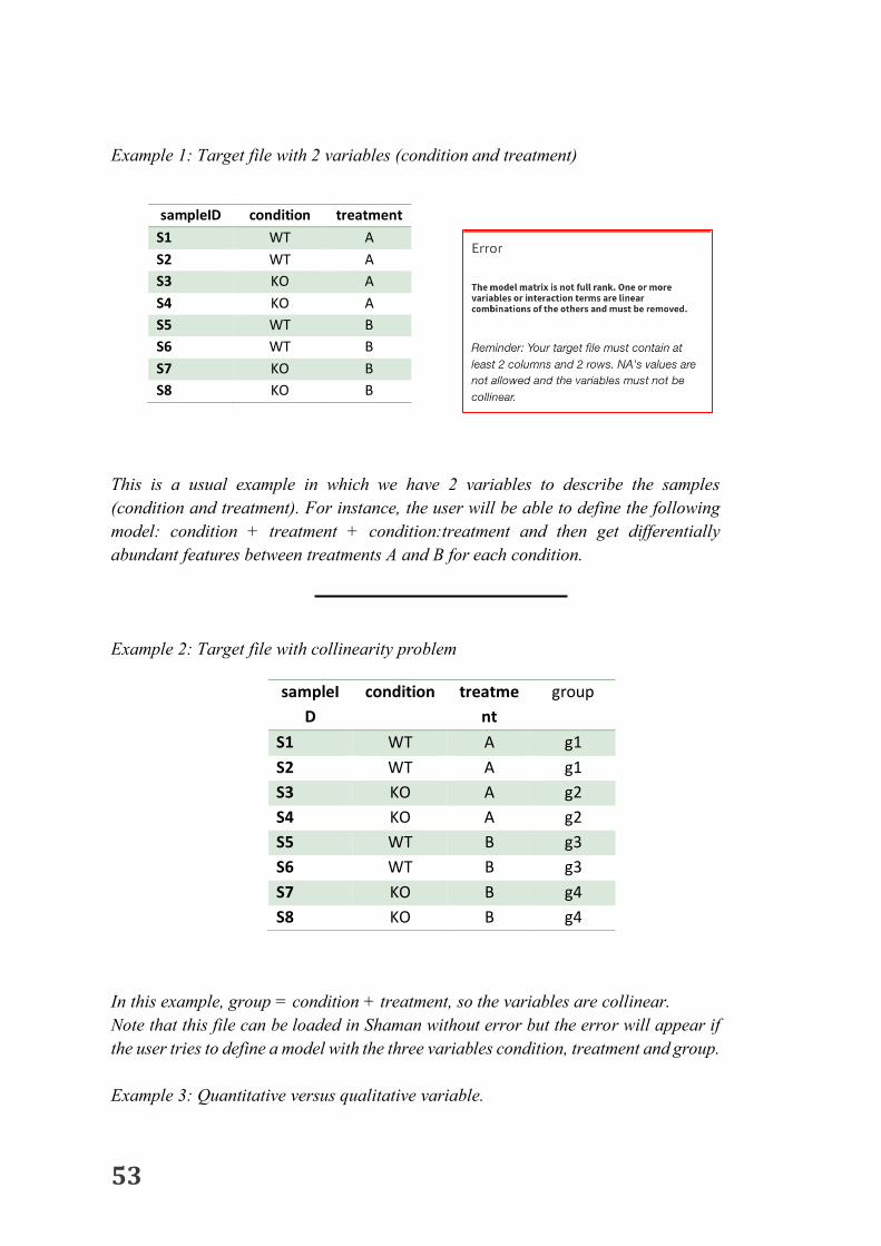
Example 1: Target file with 2 variables (condition and treatment) This is a usual example in which we have 2 variables to describe the samples (condition and treatment). For instance, the user will be able to define the following model: condition + treatment + condition:treatment and then get differentially abundant features between treatments A and B for each condition. Example 2: Target file with collinearity problem In this example, group = condition + treatment, so the variables are collinear. Note that this file can be loaded in Shaman without error but the error will appear if the user tries to define a model with the three variables condition, treatment and group. Example 3: Quantitative versus qualitative variable.

sampleID condition treatment S1 WT A S2 WT A S3 KO A S4 KO A S5 WT B S6 WT B S7 KO B S8 KO B

sampleID

condition treatment

group

S1 WT A g1 S2 WT A g1 S3 KO A g2 S4 KO A g2 S5 WT B g3 S6 WT B g3 S7 KO B g4 S8 KO B g4

54

In case 1, condition is considered as a numeric variable which leads to only one parameter in the statistical model. It assumes that the difference between 1 and 3 is two times the difference between 1 and 2 and so on. In case 2, there is no order between the conditions.

sampleID condition S1 1 S2 1 S3 2 S4 2 S5 3 S6 3 S7 4 S8 4

sampleID condition S1 C1 S2 C1 S3 C2 S4 C2 S5 C3 S6 C3 S7 C4 S8 C4

Model parameters Target file