shallow water tomography in a highly variable …

SHALLOW WATER TOMOGRAPHY

IN A HIGHLY VARIABLE SCENARIO

SiPLAB-FCT, Universidade do Algarve

Campus de Gambelas, PT-8005-139 Faro, Portugal

E-mail: {csoares,sjesus}@ualg.pt

NATO Undersea Research Centre

Viale San Bartolomeo 400, IT-19138 La Spezia, Italy

E-mail: [email protected]

In October 2000, SiPLAB and the Instituto Hidrografico (IH - PN) conducted the IN-´

TIFANTE’00 sea trial in a shallow area off the Peninsula of Troia, approximately 50 km´

south from Lisbon, in Portugal. The experiment itself and results obtained in most of

the data set have been reported at various occasions in the last two years. This paper

focuses on the data acquired during Event 2, where the acoustic propagation path was

approximately range independent and the source ship was held on station at a constant

range of 5.8 km from the vertical line array. Although these conditions were, in general,

relatively benign for matched-field tomography, retrieval of water column and bottom

parameters over a 14-hour-long recording revealed to be extremely difficult. This paper

analysis in detail the characteristics of this data set and determines the causes for the

observed inversion difficulties. Is is shown that the causes for the poor performance of

the conventional methods are mainly the tide induced spatially correlated noise and the

relative source-receiver motion during time averaging. An eigenvalue-based criterion is

proposed for detecting optimal averaging time. It is shown that this data selection pro-

cedure together with hydrophone normalization and an appropriate objective function

provide a better model fit and consistent inversion results and thus a better understanding

of the environmental variability.

1 Introduction

Ocean Acoustic Tomography (OAT) was initially proposed for deep water regions where the ray ap-

proximation was valid and sound speed could be analytically linked to acoustic ray travel-time [1].Travel-time based tomography turned out to be highly dependent on the ability to separate closely

spaced arrivals and on the precise knowledge on the source-receiver relative position at all times.

Instead, matched-field tomography (MFT) is based on some sort of correlation of the full pressure

field to the signal received at an array of sensors and only requires relative travel times to which an

© 2006 Springer. Printed in the Netherlands.

A.Caiti,N.R. Chapman,J.-P. Hermand and S.M. Jesus (eds.), Acoustic Sensing Techniques for

197

the ShallowWater Environment, 197–211.

CRISTIANO SOARES AND SERGIO M. JESUS

EMANUEL COELHO

´

198 C. SOARES ET AL.

approximate knowledge of the source-receiver position is sufficient [2]. In most operational shallow

water scenarios, only MFT is applicable due to the close arrivals from bottom and surface reflections

(IH

proximately 50 km south from Lisbon, in Portugal. The experiment itself and results obtained in part

of the data set have been reported during these last two years in various occasions [3], [4], [5], [6].This paper focuses on the data acquired during Event 2, where the acoustic propagation path was

approximately range independent and the source ship was held on station at constant range of 5.8 km

from the vertical line array (VLA). Although these conditions seem ideal for MFT, retrieval of water

column and bottom parameters over an 14 hours long recording using a focalization-like procedure

turned out to be extremely difficult and resulted in several mismatched parameter estimates.

This paper analyses in detail the characteristics of that data set and the reasons for inversion

failure. Separated eigenvalue analysis of the signal plus noise and noise only data sections revealed

that signal and noise subspaces are not well separated since the noise showed to have a strong spatial

correlation and the signal energy spread over a wide range of eigenvalues. The causes are attributed

to both source-receiver motion and tidal current forcing on the VLA. After identifying the causes,

several methods to counter these effects are proposed. In particular, a cross-frequency based ob-

jective function in conjunction with a proper selection of the data window length, according to the

variable source range, and a data normalization for correct initial phase correlation at each frequency

contributed for a decrease of the water column and bottom parameter errors. It is shown that this data

selection procedure provides a better understanding of the influence of the environment and thus final

inversion results that are consistent with independent measurements.

2 The INTIFANTE’00 sea trial

The INTIFANTE’00 sea trial was carried out on a shallow water area in the vicinity of Setubal,´

situated approximately 50 km south of Lisbon, during October 2000. This is known to be an area

of intense activity in terms of internal tides, internal waves, and river plumes. This sea trial served

several purposes: one, among others, was to study the effect of environmental variability in acous-

tic tomography through long observation times of continuous acoustic transmissions. Event 2 was

designed for this purpose, and this study will therefore focus on that data set.

The experimental area was a rectangular box situated in the border of the continental platform

with depths varying from 60 to 140 m. Figure 1 shows a bathymetric map of the northern half of the

rectangular box. The black thick line represents the track of the research vessel NRP D. Carlos I, tow-

ing the sound source, during Event 2 and extending towards the NW of the 16-hydrophone-4 m spac-

ing VLA. The bathymetry over this NW leg is considered range-independent with an approximate

average depth of 118.7 m.

The research vessel NRP D. Carlos I departed from the VLA location at time 13:30 of Julian day

289 and moved at a constant speed of 1.2 knot along NW leg during 2 hours, as depicted in Figure 1.

After an interruption for battery changing, signal transmissions resumed at time 21:00, with the NRP

D. Carlos I holding a station at approximately 5.8 km from the VLA while continuously transmitting

acoustic signals until time 11:30 a.m. of Julian day 290. The acoustic aperture of the VLA was

between 30 and 90 m. The wave form emitted during Event 2 was a 2 s duration linear frequency

modulated (LFM) sweep in the band 170 to 600 Hz with a repetition rate of 10 s.

During the INTIMATE’00 sea trial a water column temperature survey using a thermistor chain

and XBTs was conducted. The X signs in figure 1 denote the locations where the XBTs were released

every 3 hours during approximately 2 days. These data were used in this study for the computation

of the channel characteristic empirical orthogonal functions.

- PN) conducted the INTIFANTE’00 sea trial in a shallow water area off the Peninsula of Troia, ap-´

and to a perpetual source/sensor motion. In October 2000, SiPLAB and the Instituto Hidrografico

SW TOMOGRAPHY IN A HIGLY VARIABLE SCENARIO 199

Figure 1. INTIFANTE’00 sea trial site bathymetry with XBT locations and track for Event 2.

3 Acoustic tomography via matched-field

3.1 The environmental model

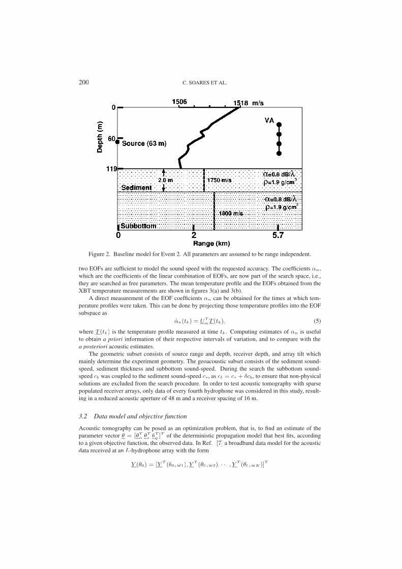
For any inversion problem in underwater acoustics, the choice of an environmental model able to

represent the properties of the propagation channel is an important step. That model, usually called

baseline model, includes the available a priori information for the problem at hand. Since there

were no in situ measurements of the seafloor properties during the experiment, a generic baseline

model was chosen. It consists of a typical three-layer model with an ocean water column overlying

a sediment layer and a bottom half-space, all assumed range independent, as shown in figure 2. For

forward model computations the parameters were divided into subsets of water column, geometric,

and geoacoustic parameters.

The water column is described by a linear combination of Empirical Orthogonal Functions

(EOFs) that are constructed from representative data sampling the depth dependence of the ocean

sound speed. The EOFs are obtained using singular value decomposition (SVD) of a matrix C with

columns

Ci = ti − t, (1)

where ti are the real profiles available, and t is the average profile. The SVD is known to be

C = UDV, (2)

where D is a diagonal matrix containing the singular values, and U is a matrix with orthogonal

columns, which are used as the EOFs. The temperature profile is obtained by

TEOF = t +

N∑

n=1

αnUn, (3)

where t is the average temperature profile, Un is the nth EOF, and N is the number of EOFs to be

combined, judged to accurately represent the temperature profile for the problem at hand. Generally,

a criteria based on the total energy contained in the first N EOFs is used. The temperature profiles

obtained from the XBT measurements (see X signs in figure 1 and profiles in figure 3(a)) served as

database for the computation of the EOFs. The criteria used to select the number of relevant EOFs

was

N = minN

{

∑N

n=1λ2

n∑M

m=1λ2

m

> 0.8}, (4)

where the λn are the singular values obtained by the SVD, M is the total number of singular values,

provided that λ1 ≥ λ2 ≥ . . . ≥ λM . For this data set the criteria (4) yielded N = 2, i.e. the first


Figure 2. Baseline model for Event 2. All parameters are assumed to be range independent.

two EOFs are sufficient to model the sound speed with the requested accuracy. The coefficients αn,

which are the coefficients of the linear combination of EOFs, are now part of the search space, i.e.,

they are searched as free parameters. The mean temperature profile and the EOFs obtained from the

XBT temperature measurements are shown in figures 3(a) and 3(b).

A direct measurement of the EOF coefficients αn can be obtained for the times at which tem-

perature profiles were taken. This can be done by projecting those temperature profiles into the EOF

subspace as

αn(tk) = UT

nT (tk), (5)

where T (tk) is the temperature profile measured at time tk. Computing estimates of αn is useful

a posteriori acoustic estimates.

The geometric subset consists of source range and depth, receiver depth, and array tilt which

mainly determine the experiment geometry. The geoacoustic subset consists of the sediment sound-

speed, sediment thickness and subbottom sound-speed. During the search the subbottom sound-

speed cb was coupled to the sediment sound-speed cs, as cb = cs + δcb, to ensure that non-physical

solutions are excluded from the search procedure. In order to test acoustic tomography with sparse

populated receiver arrays, only data of every fourth hydrophone was considered in this study, result-

ing in a reduced acoustic aperture of 48 m and a receiver spacing of 16 m.

3.2 Data model and objective function

Acoustic tomography can be posed as an optimization problem, that is, to find an estimate of the

parameter vector θ = [θTα θT

s θTg ]T of the deterministic propagation model that best fits, according

to a given objective function, the observed data. In Ref. [7] a broadband data model for the acoustic

data received at an L-hydrophone array with the form

Y (θ0) = [Y T (θ0, ω1), YT (θ0, ω2), · · · , Y

T (θ0, ωK)]T

to obtain a priori information of their respective intervals of variation, and to compare with the


Figure 3. Temperature profiles measured during the INTIMATE’00 sea trial using XBTs, and em-

pirical orthogonal functions obtained from the XBT temperature profiles (b).

= H(θ0)S + N, (6)

was proposed in order to introduce, as much as possible, a common frame for the narrow and broad-

band cases. The matrix H(θ0) is

H(θ0) =

H(ω1, θ0) 0 . . . 00 H(ω2, θ0) . . . 0...

.... . .

...

0 0 . . . H(ωK , θ0)

, (7)

where K is the number of frequencies considered and H(ωk, θ0) is the channel response for fre-

quency ωk, and the number of rows of H(θ0) is KL. θ0 is the parameter vector representing the

relevant parameters to be estimated. The vector S has entries S(ωk)α(ωk). S(ωk) is the spectrum

of the emitted waveform and α(ωk) is a generic random perturbation factor that has been discussed

in detail in Ref. [7], and was presented with the purpose of modeling small scale environmental

perturbations. This follows from the observation that repeated emissions of a deterministic signal

result in successive receptions suffering rapid changes, even at high SNR. The vector N represents

the noise assumed independent across space and frequency, and has obviously the same notation as

Y in (6).

It follows that (6) can be used directly to obtain the correlation matrix as

CY Y (θ0) = E[Y(θ0)YH(θ0)]

= H(θ0)CSSHH(θ0) + CNN , (8)

where CSS = E[S SH] is a signal matrix that measures the frequency cross-correlation of the re-

ceived signals and has entries

[CSSij= E[S(ωi)α(ωi)S

∗(ωj)α∗(ωj)]. (9)


Matrix CSS is diagonal if the frequency bins S(ωk)α(ωk) are uncorrelated across frequency. The

matrix CNN is the noise correlation matrix and is diagonal with L×L dimensional blocks σ2N (ωk)I

if the noise is uncorrelated over space and frequency. Here it is assumed that σ2N is independent of

the frequency. Equation (8) has the classical form found in horizontal array beamforming where the

signal matrix stands for the correlation of multiple emitters, while in the present case it stands for the

correlation of multiple frequencies.

The objective function used here is the cross-frequency incoherent broadband processor obtained

as

P (θ) =tr{PH(θ)CY Y PH(θ)CY Y }

tr{PH(θ)CY Y }, (10)

using the data model proposed in equation (6) and where tr{·} is the matrix trace operator. Ma-

trix PH(θ) = H(θ)[HH(θ)H(θ)]−1H

H(θ) is a projection matrix, well known from topics such

as subspace based, least mean squares, or maximum likelihood methods. Note that equation (10)

also generates auto-frequency terms. If the signal is assumed to be uncorrelated across frequencies,

and flat spectrum, i.e., CSS is assumed identity, then a processor equivalent to the conventional

incoherent Bartlett processor for K frequencies is obtained:

P (θ) =

∑K

k=1H(ωk, θ)H

CY Y (ωk)H(ωk, θ)∑K

k=1||H(ωk, θ)||2

. (11)

In practice, CY Y , given by equation (8), is replaced by a sample correlation matrix considering

N snapshots, given as

CY Y =1

N

N∑

n=1

Y n(θ0)YH

n (θ0), (12)

with Y n(θ0) containing the K data vectors Y n(θ0, ωk).

Michalopoulou [8] suggested the normalization of the received acoustic field by dividing the

received signals by the signals corresponding to the hydrophone with highest SNR, in order to over-

come the requirement of knowing the emitted waveform when a coherent processor is used. Observ-

ing the phases of the complex field received across the array, it can be found that a sensor coherent

and frequency dependent continuous drift occurs over time. Consequently, the coherence of cross-

frequency terms computed over the observation time is destroyed, causing diagonalization of the

signal matrix CSS . Normalization using a reference hydrophone can also be useful to increase the

coherence of the signals received along time, and reduce the diagonalization of the signal matrix

CSS , and therefore the spreading of energy into different eigenvectors. This data normalization is

applied during this study. However, no details on the choice of the reference hydrophone will be

given here.

3.3 Parameter focalization applied to OAT

The present estimation problem represents a case where multiple parameters are assumed to be either

unknown or known only to a certain degree. Several parameters are therefore to be optimized simul-

taneously in order to fit the model to the data via environmental focalization [9]. The water column

temperature, parameterized by the EOF coefficients, is time variant as well as source position (both

range and depth), array tilt and receiver depth. In order to reduce ambiguities, water depth is not

included as search parameter but tidal variation is accounted for using a tide prediction model and

a reference mean water depth of 118.7 m. Then, adopting the spirit of the focalization procedure, it

was decided to account for uncertainty in the seafloor properties, in order to improve the model fit.

Table 1 shows the parameters searched, with respective search bounds and quantization steps. The

search bounds reflect the use of the available a priori knowledge. For example, it was found that

by projecting the XBT temperature profiles into the EOF subspace, the measured αn are confined


Model parameter min. max. Quantization steps

Temperature

α1 (oC) -5 5 32

α2 (oC) -5 5 32

Geometric

source range (km) 5.4 6.1 32

source depth (m) 70 85 32

receiver depth (m) 85 95 32

tilt (rad) -0.045 0.045 32

Sediment

comp. speed (m/s) 1520 1680 32

thickness (m) 1 7 16

Bottom

comp. speed (m/s) 1 200 32

Table 1. GA forward model parameters with respective search interval. The compressional speed in

the bottom is coupled to the compressional speed in the sediment.

to the interval -3 and 3. However, during the data inversions a larger variation is allowed in order

to avoid obtaining estimates on the boundaries of the search intervals. A priori knowledge from the

experiment was used to restrict the search limits for the geometrical parameters source range and

source depth.

The correlation matrices were computed considering only the time series received at 4 hy-

drophones, 4, 8, 12 and 16, taking 20 frequencies from 288 to 592 Hz with a step of 16 Hz obtained

from 18 Fourier-transformed LFM sweeps, giving an acoustic observation time of ca. 3 minutes.

This procedure was repeated with intervals not shorter than 15 minutes.

-s

tricted, it is still of the order 1013. Such a huge search space can be covered using a genetic algo-

rithm (GA), which enables a significant reduction of the number of forward models to be computed.

The forward computation model used was the normal mode code C-SNAP [10] and the GA is an

implementation proposed by Fassbender [11]. The population size was set to 160 and the number

of iterations to 50. Three independent populations were run for each time point. The crossover prob-

ability was set to 0.7, initial mutation probability was 0.0096 and the final mutation probability was

0.0026, where its value was linear with the iteration number. In order to allow a more efficient search

the solution at a given time point is used in the initialization of the solving procedure of the next time

point. For more details see [4].The inversion results shown in figure 4 were obtained using the conventional Bartlett processor

(11). The left column contains the estimates of the αi (black curves) together with an interpolation

of the projections based on the measurements obtained with (5) - colored curves. It can be seen that

the αi are reasonably well estimated at the beginning of the run, taking one or two outliers apart,

but then progressively the estimates diverge from the measurements, reaching the largest error at

time 290.25. Then the αi estimates progressively start to converge again to the measured values,

where in particular α2 has some estimates coinciding with the measurements between time 290.35

at the end of the run. In the center column of figure 4, source range estimates (black curve) are of

reasonable quality, with few severe errors and most estimation errors within the GPS accuracy and

uncertainty caused by cable scopes in the moorings of the receiving system [12], while for the other

geometric parameters some difficulties are present, specially at the beginning of the run, and around

time 290.3. The geoacoustic parameters (right column) show a chaotic behavior, indicating that the

seafloor properties cannot be properly retrieved from this data set.

Although a great deal of a priori information is used to keep the size of the search space re


Figure 4. Focalization results obtained for Event 2.

The most important fact is that initially the inversion procedure reasonably yields the expected

values for the estimative of the αi, until a progressive departure between the estimates and the mea-

sured values takes place. The main question at this point is to find one or more explanations for that

occurrence. From the propagation channel point of view the question is: what has changed to cause

such degradation in the quality of the estimation results? The next section attempts to find the causes

for the fluctuation of the estimation performance observed above.

4 Datamodels and eigenvalues

Severe parameter estimation difficulties were found in part of the data analysed in the previous sec-

tion. Such difficulties are potentially generated by two types of model mismatch - physical and

statistical. The physical model mismatch can be originated by missing a priori environmental infor-

mation about the channel and geometry, causing an erroneous or too simplistic choice of the physical

model. On this side of the problem there is not much to be done since the amount of information is

fixed to that available a priori. The statistical model mismatch results from wrong assumptions on

the statistical properties of signals received on the vertical array, and thus erroneous choice of signal


or noise models. The problem at hand is to recall the statistical model in detail and to investigate

whether any of the assumptions has been violated such that the estimation process failed to yield

proper model parameter estimates.

The signal model described in (6) assumes that the field measured at the array corresponds to the

channel Green’s function as the solution of the wave equation at the sensor locations depending on

source position and environmental parameters incorporated into a channel response vector H(ω, θ0).

Noise perturbations are conveniently expressed in terms of covariance matrices CUU , which describe

the ocean noise spatial and frequential structure. For the derivation of the matched-field processor

in equation (10), it was assumed that the signals were random frequency cross-correlated and that

the noise is uncorrelated across space and frequency, falling in the category of sensor noise with a

diagonal structured covariance matrix.

The eigendecomposition of the covariance matrix in equation (8) can be of central importance,

since the eigenvalues are a mirror of its structure and its positivity allows for the factorization in

eigenvalues and eigenvectors

CY Y (θ0) = VEVH

, (13)

with V unitary and E = diag{e1, e2, . . . , eKL} a diagonal matrix of real eigenvalues ordered such

that e1 ≥ e2 ≥ . . . ≥ eKL > 0. In the case of uncorrelated noise, it can be observed that if the

signal matrix CSS has full rank then there will be L(K−1) eigenvalues equal to σ2U . If, on the other

hand, CSS has rank equal 1, then the signal component is deterministic and LK − 1 eigenvalues are

equal σ2U . In terms of matched-field processing this is the most convenient case, since it corresponds

to matching the replica to the eigenvector associated with the largest eigenvalue of matrix CY Y .

The ratio between the first and second eigenvalues ( e1

e2

) is often an indicator of the adequateness

of the statistical model relative to the data being processed.

In terms of eigenvalue analysis it is suitable to observe the eigenspectrum of the sample corre-

lation matrix, in particular the behavior of the ratio between e1 and e2. This gives a measure of the

degree of dominance of the first eigenvalue over time in order to detect changes in the structure of

the data, and evaluate its disagreement relative the assumed model. The advantage of the eigenvalue

analysis is that it is data-consistent, since it only depends on the received signals.

Figure 5(a) shows the eigenspectra of the sample correlation matrix versus time, with a data gap

due to an interruption for changing the batteries of the VLA. Before and shortly after the data gap,

the ship is moving away from the VLA location where it can be seen that the eigenspectra energy

is spread out reaching significant values up to order 10/12. This is clearly due to a violation of the

channel stationarity assumption for cross-covariance matrix estimation where several different chan-

nel acoustic responses were averaged together within the data window. After time 289.9 the source

ship is free drifting so movements are limited to those necessary to keep the station. Surprisingly a

significant energy spreading can also be noticed in the time interval 290 to 290.35 (approximately

9 hours), after which it abrupbtly falls off. Along the whole interval some spikes are also visible,

which can be attributed to ship movements to maintain the station. In order to obtain a quantitative

measure of the energy spreadout figure 5(b) shows the evolution of the e1

e2

ratio (top) and its inversee2

e1

(bottom). It is clearly visible that the movement of the source ship in the first part of the run

strongly reduces the e1

e2

ratio, that immediately increases when the ship stalls. As expected from the

eigenspectra data an abrupt reduction of the e1

e2

ratio can also be noticed in the time interval 290 to

290.35. While it is easily understandable that the e1

e2

ratio remains low while the ship is moving fast,

it is not so clear why this ratio remains low in the interval 290 to 290.35 during which the ship was

on station and the acoustic channel responses should be relatively stable or do not suffer significant

changes during the 3 min averaging window for each covariance matrix estimation. Clearly, the

cause for the abrupt decrease of the e1

e2

ratio in that time interval is not the same as it is before the

gap, neither the is the effect the same.

Thus there might be several effects causing these high variations in the spreading of the eigen-

spectrum. To some extent such spreading might be caused by a disagreement between the received


(a) (b)

Figure 5. Eigenspectra computed from the cross-frequency correlation matrix (a); ratio between the

two greatest eigenvalues e1

e2

(b - top) and e2

e1

(b-bottom).

data and the statistical model assumed for the present problem. The rate of change in the degree of

spreading at some time points configures this data set as being acquired in a highly variable scenario.

The next step is to search for possible causes that can explain this model - data disagreement.

4.1 Acoustic source motion

The parameters concerning the source position are leading parameters in terms of acoustic field sen-

sitivity. Thus one must account for variations in the source position during the signal emissions. In

the present case the repetition rate of the emitted signal is 10 s. The number of snapshots used to

compute the sample correlation matrix is a compromise between its variance and the time coherence

of the propagation channel. A number of snapshots equal to 18 represents about 3 minutes of ob-

servation time. This means that the hypothesis of a time-invariant propagation channel can possibly

be violated for a given acoustic source motion. From the statistic point of view and in terms of

eigenvalues, the variability of the acoustic response will induce a loss of dominance of the largest

eigenvalue, due to energy partitioning in different eigenvectors. The gray line of the range vs. time

plot of figure 4 reveals that the source ship was moving quite often struggling to keep the station,

while being pushed towards the VLA by wind and currents. Ship motion not only implies a change

on source range, but also in source depth, since, for a fixed cable scope, the source depth is a function

of ship speed according to its characteristics. Thus, during accelerations, changes in the source depth

occur. Figure 6(a) shows the ship speed at discrete times when acoustic data was received, and figure

6(b) shows the correlations of ship speed and ship acceleration with the e2

e1

ratio vs. time (figure

5(b-bottom)). The time axis of the correlation plot is actually in time bins (for a total number of 232)

since there is a gap in the data the time bins are not uniformly spaced. It can be seen that the level

of e2

e1

is strongly correlated with the ship speed yielding a correlation above 0.9 and with the peak

perfectly placed in the center of the plot, i.e., for a time lag equal to zero. The influence caused by the

ship acceleration is more difficult to detect since the change in speed occurs for very short periods of

time and involves a second order derivative of the position record, prone to instabilities. However,

the maximum correlation still appears at the center of the function. In the present case, the source

motion problem can be seen as a short time scale phenomenon. In figure 5(b) it can be clearly seen

that some spikes in the e2

e1

ratio are standing out at several times, and those can be atributed to source

motion. However, the overall energy spreading can not be accounted for by acoustic source motion

only, which lead us to search for other environmental related causes.


(a) (b)

Figure 6. Correlation of ship speed and acceleration functions with the e2

e1

function shown in figure

5(b).

4.2 Noise level and tidal forcing

Recalling the discussion on eigenvalue analysis in the first half of section 4, it appears that the overall

energy spread of the eigenspectrum in the interval 290 to 290.35 could be due to a structured noise

background superimposed by short time scale variations due to source ship motion as described in

the previous section.

Figure 7(a) shows a noise power estimate for hydrophone #1 as a function of time and frequency.

Here the abrupt change in noise level in the time interval 290 to 290.35 is quite clear with several

strong lines across the whole frequency band, however, with some predominance below 350 Hz.

Observing the colorbar it is also found that the fluctuation of the noise level is up to 30 dB. Finally,

in figure 7(b), that shows the noise eigenspectra along time, it can be seen that the noise power

abrupt changes are accompained by statistical changes denoting a correlated signal-like structure in

the target interval 290 - 290.35. The noise covariance matrices show strong spatial noise correlation

in that period of time, which by itself is a potential reason for the breakdown of the inversion process.

It remains to find out what originated such high noise amplitude and correlation. There are

several possible noise origins in the ocean. The most common is ambient noise caused by waves

or wind at the ocean surface that translate in a correlated noise field at the vertical array. Other

common source of correlated noise is that due to distant shipping but generally manifest itself as a

variable spectrum strongly attenuated at frequencies above, say, 200 Hz - which obviously is not the

case here. Flow noise and mechanical vibration are also common sources of noise when addressing

horizontal towed arrays or vertical arrays in strong currents. Although there are no recordings of the

current field during the experiment, historical records show that tidal driven currents up to 2.5 m/s

were measured in the area. Figure 7(c) shows a plot of the estimated noise level and the absolute

value of the tidal forcing superimposed. The tide was predicted using a tide prediction model. It is

not quite obvious that the noise level increases with the tidal forcing, but a correlation between these

two quantities reveals that they are in fact strongly correlated, reaching a maximum correlation over

0.8 for zero time lag (figure 7(d)). If the current is sufficiently strong it can cause the VLA line to

vibrate between the mooring and the surface buoy. In that case the vibrations can origin mechanical

noise propagating along the VLA sensed by the hydrophones and resulting in spatially structured

noise over a large frequency band.


(a) (b)

(c) (d)

Figure 7. Estimated noise level as a function of time and frequency (a); eigenspectrum of a full rank

noise covariance matrix as a function of time (b); average noise level estimated using all hydrophone

with absolute tide force value over time (c); correlation of estimate noise level with absolute tide

force (d).

5 Data quality improvement for inversion

In the sections above it was shown that various factors have a significant impact on the data structure

and therefore on the inversion process. It could be seen, e.g., that if during the observation time

the environment or the geometry suffers strong changes, it is likely that the energy received along

time at the array tends to be spread into different eigenvectors. This is equivalent to observing a

decorrelation of consecutively received signals. The duration of the observation window establishes

a trade-off between the coherence of the propagation channel and the variance of the covariance

matrix estimate. To handle fast varying environments one can implement an eigen-based processing

technique simply based on the maximization of the e1

e2

ratio with the goal of adaptively determining

the observation time. Ideally, this would measure the relative decorrelation rate between signals and

noise.

On the other hand, high level and spatially correlated noise have shown to be an important diffi-

culty during part of the experiment. An additional factor of difficulty is the change of the noise struc-

ture along time, where the estimated degree of cross-correlations has shown a significant variation,

leading to the failure of the assumption of spatially uncorrelated noise. In that case the straight step

is to gain knowledge on the noise structure and use it in the derivation of a matched-field processor

assuming structured noise. Cross-frequency processors can explore the advantage of the stochastic

independence of frequency bins in the frequency domain, as the result of a discrete Fourier transform


Cross Eig. SS Eig. Norm

Case 1 No No No

Case 2 Yes No No

Case 3 Yes Yes No

Case 4 Yes Yes Yes

Table 2. Summary of the four processing cases. Cross stands for cross-frequency processing; Eig.

SS stands for maximization of the e1

e2

ratio as a function of the number of snapshots; Eig. Norm

stands for maximization of the e1

e2

ratio as a function of normalizing the data by the best hydrophone.

property (see [7] for a complete description of the noise handling assumptions of the cross-frequency

processor).

The remaining part of this section describes an attempt to improve the quality of the estimates

by mitigating the difficulties discussed above. Three additional inversion results are being reported,

where processing features are successively added. Four cases are summarized in table 2:

• Case 1 corresponds to the inversion reported in section 3.3 where the conventional processor is

used;

• Case 2 corresponds to the application the cost function presented in equation (10), with a con-

stant number of snapshots equal 18 and performing normalization to the best hydrophone. The

idea is to take advantage of the reduced noise correlation across frequencies, since it has been

observed that in part of the run extremely strong spatial noise correlation is present;

• Case 3 where the number of snapshots used for each covariance matrix is variable according

to the maximization of the e1

e2

ratio, in order to inspect whether the variability seen during the

observation window is a source of loss in parameter estimation performance, and finally

• Case 4 where the eigenvalue ratio is tested against the decision of normalization or not. The

problem being addressed in this case is that of coping with drifts of the phases of the acoustic

field, that prevent the field being summed coherently during the computation of the cross-

correlation matrix.

As an example of Case 3, figure 8(a) shows the result of the maximization with respect to the number

of snapshots N vs time. The effect of source motion at the beginning of the run is perfectly visible,

both before and after the data gap. Then as the ship stalls a raise in the estimates of N is observed.

During the rest of the run some variability in N can be seen. Figure 8(b) shows that the estimates of

N are strongly correlated with ship speed and acceleration. One interesting remark is that the corre-

lation functions in figure 8(b) have a very similar shape of those of figure 6(b), possibly indicating

that there is a close relation between the estimates of N and the e1

e2

ratio.

The inversion results obtained along the four cases are summarized in table 3 in terms of root

mean square error (RMSE) for the parameters that can be measured and are subjected to change with

time, and in terms of standard deviation for the seafloor parameters that are unknown but assumed

to be invariant along the whole run. Although not perfectly monotonic, it can be observed that

from case 1 to case 4, an improvement can be observed for each new feature introduced in the

processing. Although the improvement seems to be small, there is clearly a tendency to ameliorate

the estimation quality, especially in cases 3 and 4. The cross-frequency processor appears to perform

better in conjunction with the eigen-based processing introduced in cases 3 and 4. The introduction

of the cross-frequencies in case 2 by itself has shown little or no improvement to the estimation,

since the length of observation time is not addressed and the noise appears to have some frequency

cross-correlation. The estimation results obtained in case 4 are not shown graphically, since, visually,

it would be difficult to take striking conclusions.


(a) (b)

Figure 8. Estimated number of snapshot over time and its inverse (a); Correlation function of the

inverse of the estimated N with ship speed and acceleration (b).

Proc. RMSE1 Std. dev2

Rs α1 α2 cs h cb

(km) (◦C) (◦C) (m/s) (m) (m/s)

case 1 0.125 2.289 1.458 36 1.65 78

case 2 0.126 2.283 1.253 38 1.48 80

case 3 0.121 2.130 1.161 35 1.45 69

case 4 0.117 2.055 1.204 28 1.40 62

Table 3. Inversion performance measured via: 1 RMSE using GPS source-receiver range and and

XBT projected EOF coefficients; 2 standard deviation of seafloor parameters (compressional velocity

in sediment and subbottom, sediment thickness).

6 Conclusion

In scenarios where a great deal of information is available, matched-field methods are highly reliable.

Thus, they are suitable to be applied to OAT, where the number of unknown parameters is potentially

high.

The INTIFANTE sea trial, conducted in the vicinity of Setubal in October 2000, served among´

others, the purpose of acquiring data for testing OAT at ranges up to 6 km in a range-independent

shallow water environment. When compared to other more complex scenarios this appeared to be

a relatively easy task for MFT inversion of water column properties. Indeed during part of the run

the inversion of the water temperature profile provided consistent results. However, in a relatively

benign portion where the source ship was maintaining a station at 5.8 km distance from the VLA,

the estimations significantly departed from the expected results. The search for the causes of this

intriguing performance was the motivation of this paper that took us through various subjects such

as the influence of rapid source motion within the limits of the stationarity assumption and the role

of highly correlated noise possibly due to tidal flow at the array site. During the study the problem

was identified but its origin was not completely understood.

Several processing schemes were implemented in an attempt to compensate these influences.

First it was supposed that the overall quality of the data entering the inversion could be ameliorated

by using cross-frequency covariance matrices. This resulted in little improvement, since the strong

spatial noise correlation extended to the cross-frequency data as well. Then, in two additional at-

tempts an eigenvalue approach was tested in order to improve the data quality. It was shown that

energy partitioning into different eigenvectors was caused by source motion during the observation


time defined a priori. This was mitigated by optimizing the e1

e2

ratio for observation time and data

normalization. It could be shown that the estimator for the best number of snapshots was highly

correlated with the ship speed and acceleration. The inversion results could be progressively im-

proved remaining, however, strongly limited by the high noise level. Further work is necessary to

treat this problem should be treated in terms of spatial filtering by making use of a prior estimated

noise structure.

References

1. Munk W., Worcester P. and Wunsch C. Ocean acoustic tomography. Monographs on mechan-

ics. University Press, Cambridge, (1995).

2. Tolstoy A. and Diachok O., Acoustic tomography via matched field processing. J. Acoust. Soc.

Am. 89(3), 1119–1127 (1991).

3. Jesus S. M., Coelho E., Onofre J., Picco P., Soares C. and Lopes C., The intifante’00 sea

trial: preliminary source localization and ocean tomography data analysis. In Proc. of

the MTS/IEEE Oceans 2001, Hawaii, USA, November (2001).

4. Jesus S. M., Soares C., Onofre J. and Picco P., Blind ocean acoustic tomography: experimental

results on the intifante’00 data set. In Proc. of the European Conference of Underwater

Acoustics, Gdansk, Poland, June (2002).

5. Jesus S. M., Soares C., Onofre J., Coelho E. and Picco P., Experimental testing of the blind

ocean acoustic tomography concept. In Impact of Littoral Environmental Variability on

Acoustic Predictions and Sonar Performance, Lerici, Italy, September (2002).

6. Jesus S. M. and Soares C., Blind ocean acoustic tomography with source spectrum estima-

tion. In Proceedings International Conference on Theoretical and Computational Acous-

tics, Hawaii, USA, August (2003).

7. Soares C. and Jesus S. M., Broadband matched field processing: Coherent and incoherent ap-

proaches. J. Acoust. Soc. Am. 113(5), 2587–2598 May (2003).

8. Michalopoulou Z.-H., Source tracking in the Hudson Canyon experiment. J. Comput. Acoust.

4, 371–383 (1996).

9. Collins M. D. and Kuperman W. A., Focalization: Environmental focusing and source localiza-

tion. J. Acoust. Soc. America 90, 1410–1422 (1991).

10. Ferla C. M., Porter M. B. and Jensen F. B., C-SNAP: Coupled SACLANTCEN normal mode

propagation loss model. Memorandum SM-274, SACLANTCEN Undersea Research Cen-

ter, La Spezia, Italy (1993).

11. Fassbender T., Erweiterte genetische algorithmen zur globalen optimierung multimodaler funk-

tionen. Diplomarbeit, Ruhr-Universitat, Bochum, (1995).¨

12. Felisberto P., Lopes C. and Jesus S. M., An autonomous system for ocean acoustic tomography.

Sea Technology, 45(4), 17–23 (2004).

shallow water tomography in a highly variable …

Documents