Shale Boom’s Remaking of Electricity, Transportation and Manufacturing

Markets

Kenneth B Medlock III James A Baker III and Susan G Baker Fellow in Energy and Resource Economics, and

Senior Director, Center for Energy Studies, James A Baker III Institute for Public Policy Adjunct Professor, Department of Economics

Rice University

September 10, 2013

James A Baker III Institute for Public Policy Rice University

Presentation at Governors’ Policy Forum on Shale Energy Development

The “50,000 Foot” view in 2000: LNG is coming to North America

The difference a decade makes: Over 6,600 tcf of technically recoverable shale*

Major North American Shale Plays (~1,930 tcf)

European, Latin American, African and Pacific Shale Plays

(~4,670 tcf)

*Over 6,600 tcf of shale according to ARI report, 2011

Will there be growth in Foreign Supply (Shale)? Maybe, but the US is Unique.

• Stable and conducive regulatory and institutional frameworks. - Resource Access – mineral rights ownership; acreage acquisition;

resource assessments; environmental opposition; etc. - Market Structure – transportation regulation (unbundled access vs.

incumbent monopolies) and bilateral take-or-pay obligations vs. marketable rights; existence of infrastructure; pricing paradigms; etc.

• Many other issues face shale development. - Water – use in production; water rights and management; flowback

options (recycle and/or treatment and disposal) and native infrastructure; concerns about watershed protection (casing failures and fracture migration); etc.

- Other issues – earthquakes related to injection of produced and treated water; long term effects of methane escape; concerns about contamination from produced water; ecological concerns over land use and reclamation; etc. 4

Broad Implications of US Shale Gas • Expansion of production from US shale plays has rendered the

utilization of LNG import capacity in the US very low. • It has had an impact on the relative price of oil and gas, and it

has raised the possibility of US LNG exports. • But, when weighing all demand responses, and thus market

impacts, the focus should not be on just exports. • Shale gas makes the supply curve more elastic. This mitigates

the potential for sustained long term increases in price and has implications for fungibility and price volatility.

• This has bearing on many margins of demand response. • Indeed, multiple sectors are important for the longer term

implications of shale. 5

Modeling Well Decline in Shale Plays: Assessing the Long Term Potential

6

Is Production Sustainable?

7

• Well-specific EURs can vary within a shale play substantially - Ultimately, profitability matters, as there is little debate about resource scale - Example shown is Barnett Shale. We see that some wells are profitable at $2.65,

others need $8.10… median is $4.85.

EUR 2.83 bcf 1.51 bcf 0.93 bcf

Margins of Long Term Demand Response

8

Larger Supply Elasticity allows a lot of Demand Response

9

Demand increase due to exports

Q

P

Price increase due to exports

Demand increase due to exports, transport,

industry, and/or power generation

Price increase associated with higher

demand

• What if many factors come together at once (LNG, industrial demand, power generation, transportation)?

• A problem of many margins. • First-mover matters!

− How much LNG will be exported?

− How much oil can gas replace in transport?

− How much coal will be displaced in power?

− Etc…

Impact of Shale on Henry Hub, 2011-2040 • The domestic supply curve is much more elastic as a result of shale gas

developments. Domestic long run elasticity*

- with shale = 1.52; without = 0.29.

10

* - Results derived from the Rice World Gas Trade Model (RWGTM). The RWGTM was developed by Ken Medlock and Peter Hartley at Rice University using the MarketBuilder software provided by Deloitte MarketPoint .

LNG Exports

11

LNG Exports… Why the Interest? • International price is high, but will this persist?

- Unexpected demand shocks have had an influence. - It is reasonable to expect that US price will rise to reflect marginal cost

and JKM premium will subside with relief of deliverability constraint

12 Price data from Platts; LNG Oil-Index author’s calculation

Price Impacts of US LNG Exports: Don’t Forget the Foreign Market Response

• Trade affects price in both markets, the degree to which depends on relative elasticities of supply and demand.

• If supply is constrained in the importing market, the reaction there is much more pronounced.

13

τ

Domestic Market Q

P

D

S

D + x

PTd

Exports, x

Foreign Market Q

P

D’

S’ S’+ m

PTf Imports, m

Feasibility of US LNG Exports • Lots of weight given to current international spot

price, but several factors are often ignored, such as - short term capacity constraints, which are important

when considering where we are today, - domestic market interactions with markets abroad, and - a weak US dollar.

• US LNG exports could put significant downward pressure on international price. - In 2012, LNG trade was about 30 bcfd. Current filings

exceed 30 bcfd. • Prices will adjust, and greater liquidity will alter the

market paradigm in a substantial way. 14

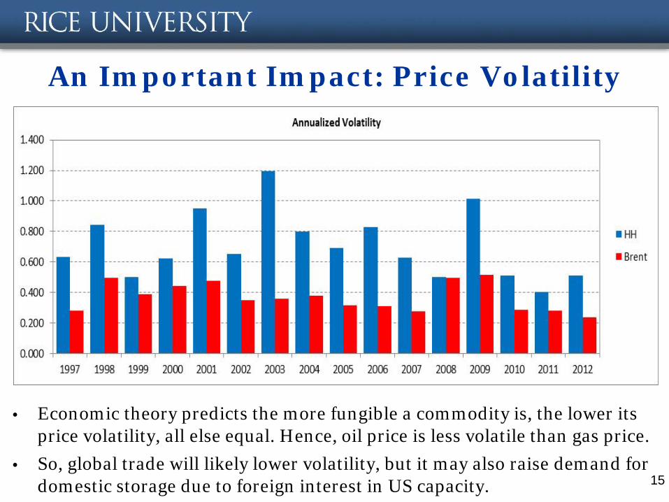
An Important Impact: Price Volatility

15

• Economic theory predicts the more fungible a commodity is, the lower its price volatility, all else equal. Hence, oil price is less volatile than gas price.

• So, global trade will likely lower volatility, but it may also raise demand for domestic storage due to foreign interest in US capacity.

Transportation

16

Transportation: The CNGV option • Consumers must see a clear benefit to changing

vehicle type/technology. So, let’s consider this… – One thousand cubic feet of natural gas yields eight gallons

of CNG. Thus, if natural gas price is $4/mcf then the cost of natural gas as a feedstock for CNG production is $0.50/gallon. Adding the processing costs for CNG of approximately $1.00/gallon, we have an estimated wholesale price of $1.50/gallon.

– The wholesale gasoline price is about $3.00/gallon. – Assuming profit margins, taxes and other costs from the

rack to retail are similar across gasoline and CNG, we have a price gap of about $1.50/gallon.

• This is a large gap!

Transportation: The CNGV option (cont.) • The fuel savings over a 7 year period is dependent

upon the basis for comparison – We will compare to a gasoline hybrid motor vehicle, since

that is the most efficient option among new vehicles. – Consider the Honda Civic model year 2013

• The gasoline hybrid engine efficiency of 44 miles per gallon in the city. • The CNGV has a city driving efficiency of 27 miles per gallon. • Thus, the cost per mile is $0.0126 lower for the Civic CNGV. • Assuming annual driving of 12,000 miles, the fuel savings is $151/year. • A 7 year life yields an undiscounted lifetime savings of just over $1,060. • The current MSRP for a Civic CNGV is $26,305, and the current MSRP for a

Civic Hybrid is $24,200, meaning the price difference is currently $2,105. Thus, the fuel cost savings does not compensate the higher upfront cost of the vehicle. If we discount future savings, the disparity grows.

Transportation Options that make Sense • Fleet Vehicles

– High mileage renders the option more sensible. But, we do need to consider the rate “behind the fence” as the LDC costs raise price. Moreover, taxing gas as a transport fuel will at some point have to be brought into the equation.

• Long Haul Trucking – High mileage again matters. Investments being made and

fuel costs may benefit from wholesale market pricing due to locations along interstates.

• Marine transportation – EPA rules will force the use of less polluting fuels near

ports. Industry is already preparing for the use of LNG to replace bunker fuel and fuel oil.

The Full Demand Response: Bringing in Power Generation and

Industrial Demand

20

The Full U.S. Demand Response... • What are the end-uses where demand could change?

- Power generation - Industrial uses as an energy source and feedstock - Automotive transportation – personal and commercial - Marine transportation – EPA forcing out heavy fuel oil and diesel - LNG and pipeline exports (foreign demand for US gas)

• Incremental demand responses (by 2020 35 bcfd) - LNG exports (12 bcfd) - Power generation (10 bcfd) - Industrial uses (7 bcfd) - Automotive transportation (2 bcfd) - Marine transportation (2 bcfd) - Pipeline exports (2 bcfd)

21

The Full U.S. Demand Response... • What are the end-uses where demand could change?

- Power generation - Industrial uses as an energy source and feedstock - Automotive transportation – personal and commercial - Marine transportation – EPA forcing out heavy fuel oil and diesel - LNG and pipeline exports (foreign demand for US gas)

• Incremental demand responses (by 2020 35 bcfd) - LNG exports (12 bcfd) < 4 bcfd – market

- Power generation (10 bcfd) < 5 bcfd – policy and market

- Industrial uses (7 bcfd) < 4 bcfd – market

- Automotive transportation (2 bcfd) < 0.15 bcfd – market

- Marine transportation (2 bcfd) < 1 bcfd – policy

- Pipeline exports (2 bcfd) < 2 bcfd – market

• Scale of demand increase < 15 bcfd – RWGTM modeled outcomes

- … or close to 25% of current demand. (Note: Res/Comm falls by >1.5 bcfd) 22

The Prospects for Light Tight Oil

23

Ongoing developments in Tight Oil • Resource potential in North America is distributed widely.

- For example, North Dakota (Bakken), Texas/New Mexico (Permian – Avalon, Bone Springs, Wolfcamp, South Texas – Eagleford), Ohio (Utica), Pennsylvania (Marcellus), Colorado/Wyoming (Niobrara), Florida (Sunniland), Louisiana (Tuscaloosa Marine), Oklahoma (Mississippi Lime), California (Monterrey). o Just as in gas, not all shales are created equal. o Bakken and Eagleford currently accounts for most US LTO production. o Internationally, shale oil resources could total over 260 billion barrels,

according to the recent ARI-EIA (2013) report.

• Technical and cost hurdles exist, as do impediments from regulatory and institutional frameworks.

• Growing US oil production has significant implications for global markets, including (1) Brent-WTI spread, (2) US import demand, and (3) US foreign policy. 24

The Shift in US Oil Production • The US entered a period of decline after the early 1970s not because it was out of

oil, but because there was a cheaper alternative: imports. • The last 5 years higher price has motivated exploration and development, leading

to a resurgence in US oil production, from unconventional and old fields. • US Oil Exports – The Next Big Washington Debate?

Source: EIA

Questions/Comments

26