shadows in games and simulations
TRANSCRIPT
Real-Time Shadows in Video Games
Amit Ofer 11-27-2016

1
Table of Contents Abstract ........................................................................................................................................... 2
1. Introduction ................................................................................................................................ 2
1.1. Hard shadows vs. soft shadows ............................................................................................ 5
2.1. Projection shadows .................................................................................................................. 6
2.1.1. Planar shadows .................................................................................................................. 6
2.1.2. Shadow Textures ............................................................................................................... 9
2.2. Shadow mapping .................................................................................................................... 11
2.2.2. Omnidirectional shadows maps ...................................................................................... 15
2.3. Shadow volumes..................................................................................................................... 16
2.3.1. Naïve implementation ..................................................................................................... 17
2.3.2. Stencil Shadow Volumes ................................................................................................. 18
2.3.3. Silhouette-Based Shadow Volumes ................................................................................. 19
2.3.4. Level of Details ................................................................................................................ 19
3. Soft shadows techniques ........................................................................................................... 20
3.1. Image based approach ....................................................................................................... 20
3.1.1. Combination of several point based shadow images ...................................................... 20
3.1.2. Fixed sized penumbra filtering techniques ..................................................................... 21
3.1.3. Variable sized penumbra filtering techniques ................................................................ 21
3.2. Geometry based approach ................................................................................................. 22
4. Conclusion and further reading ................................................................................................. 24
5. References ................................................................................................................................. 25

2
Abstract Shadows are an important part in video games and simulations, shadows contribute to realism
and help us comprehend spatial relationships between objects and where they are located
inside the scene. Furthermore, shadows can also be treated as artistic means and many movies
(and sometimes video games) exploit shadows to illustrate the presence of a person or an
object without revealing its actual appearance.
Although shadow algorithms and techniques have been researched for a few decades they still
remain a challenge for real time graphics, as new hardware is being develops games become
more realistic which demands better and quicker shadow techniques.
In this summary, I will explore and give a brief survey of the most common techniques in
shadow calculation for games and real time simulations; I will give explain the basics of 4
common shadows techniques used today: Planar shadows, Shadow Textures, Shadow maps and
shadow volumes; I will explore the differences between hard and soft shadows and discuss
some of the common approaches used to create real-time soft shadows.
1.Introduction
A shadow is defined as a dark area where light from a light source is blocked by an opaque
object.
Shadows are created when a surface blocks the light's path. The shadows caused by an ideal
point light source would be sharp but in the real world shadows have blurry edges, this is called
the penumbra. A penumbra arises because real world light sources cover some area and so
produce light rays that gaze the edges of an object at different angles.
Shadows play an important role in computer graphics. Besides dramatically improving image
realism they also provide the observer with visual cues that gives information about the viewed
scene such as the characters of the geometries, relative position of object, complexity of the
shadow occluders and receivers, shape and size of the light sources in the scene and more.
Shadows are an important component in computer graphics because they give the observer
important visual cues such as information about light sources and objects, depth perception and
light intensity.

3
Figure 1: the exact same object in all 4 images looks as if it is found in different height thanks to the shape and position of the shadow.
Figure 2:demonstrate how the shadow can give us visual cues to where the light source is located in our scene.
4
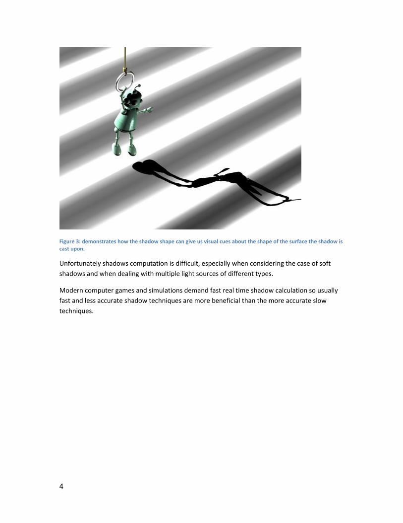
Figure 3: demonstrates how the shadow shape can give us visual cues about the shape of the surface the shadow is cast upon.
Unfortunately shadows computation is difficult, especially when considering the case of soft
shadows and when dealing with multiple light sources of different types.
Modern computer games and simulations demand fast real time shadow calculation so usually
fast and less accurate shadow techniques are more beneficial than the more accurate slow
techniques.
5
1.1.Hard shadows vs. soft shadows Shadows that are produced from point light sources (sources that has no actual size but omit
light from a 3d point in space, e.g. point light or a basic spot light) are called hard shadows.
Hard shadows have crisply defined, sharp edges as opposed to soft shadows which are created
from light sources that contains size definition such as an area light and appear less distinct and
fade out towards the edges of the shadow area.
When talking about soft shadows we divide the shadow region into two sections called umbra
and penumbra, the umbra is the innermost and darkest part of the shadow where the light
source is completely blocked by the occluding body whereas the penumbra is the region in
which only a portion of the light source is obscured by the occluding body, the width of the
penumbra is determined by the size of the light and its distance from the shadow caster and
the receiving object. In hard shadows the umbra takes the entire shadow.
Using soft shadows can make a scene appear more realistic than a scene where only hard
shadows are used but getting accurate soft shadows can be complicated to achieve, especially
when talking about games and real time simulation where computation time is usually more
important than accuracy.
Usually to get the best results, the best approach would be to use soft shadows in conjunction
with hard shadows, and prefer method for less accurate but faster soft shadows in order to
allow the scene to be rendered as fast as possible.
*note that while shadows are important to achieve realism it is only one of many effects
simulated in a computer game and thus are allowed only a limited time for computation.
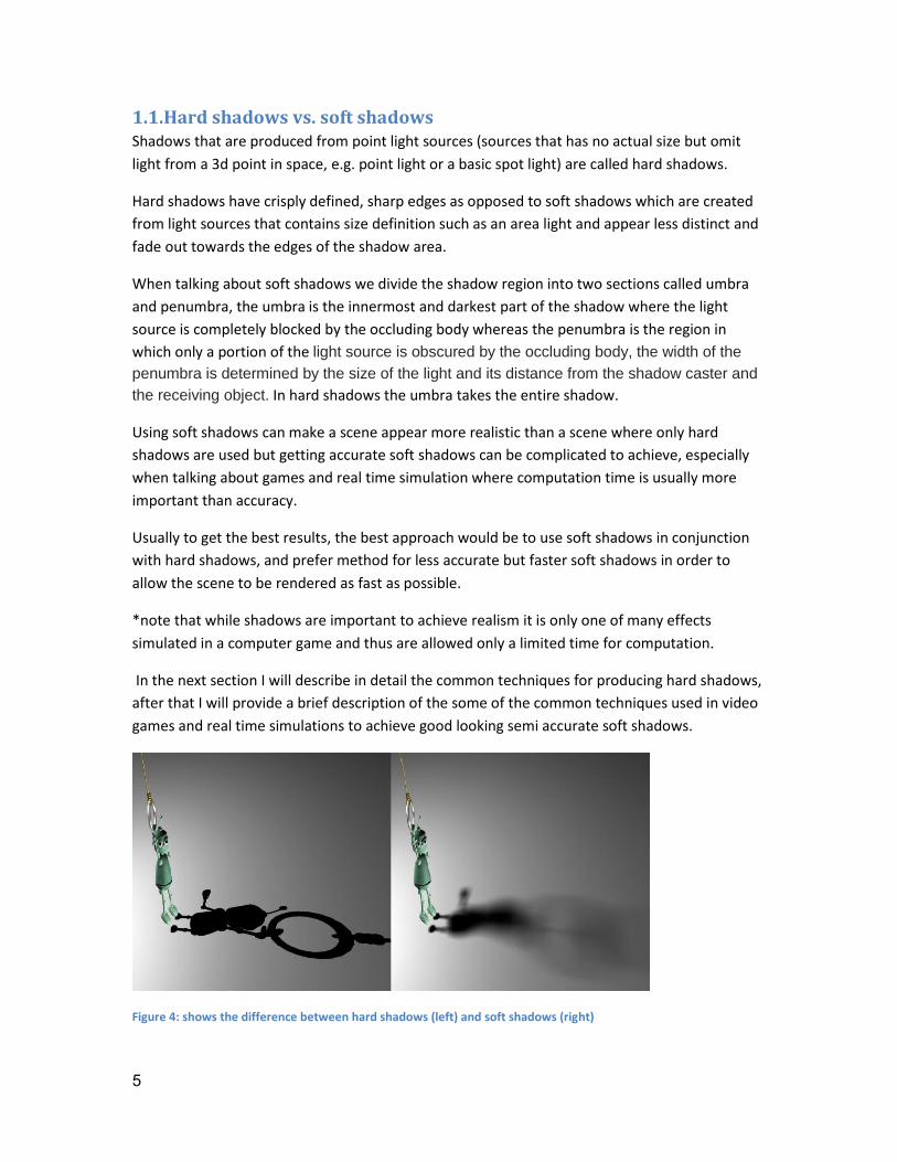
In the next section I will describe in detail the common techniques for producing hard shadows,
after that I will provide a brief description of the some of the common techniques used in video
games and real time simulations to achieve good looking semi accurate soft shadows.
Figure 4: shows the difference between hard shadows (left) and soft shadows (right)
6
2.Basic Techniques
2.1.Projection shadows Projection shadows refers to a group of relatively simple techniques that can produce good
results but suffers from several shortcomings which makes them a bit out dated in recent
rendering engines, but are still worth mentioning.
These techniques are still relevant when artistic freedom such as changing the shape, color and
texture of the shadow is more important that physical accuracy.
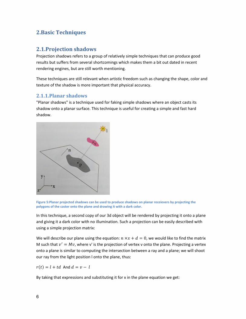
2.1.1.Planar shadows "Planar shadows" is a technique used for faking simple shadows where an object casts its
shadow onto a planar surface. This technique is useful for creating a simple and fast hard
shadow.
Figure 5:Planar projected shadows can be used to produce shadows on planar receievers by projecting the polygons of the caster onto the plane and drawing it with a dark color.
In this technique, a second copy of our 3d object will be rendered by projecting it onto a plane
and giving it a dark color with no illumination. Such a projection can be easily described with
using a simple projection matrix:
We will describe our plane using the equation: 𝑛 ×𝑥 + 𝑑 = 0, we would like to find the matrix
M such that 𝑣′ = 𝑀𝑣, where v' is the projection of vertex v onto the plane. Projecting a vertex
onto a plane is similar to computing the intersection between a ray and a plane; we will shoot
our ray from the light position l onto the plane, thus:
𝑟(𝑡) = 𝑙 + 𝑡𝑑 And 𝑑 = 𝑣 − 𝑙
By taking that expressions and substituting it for x in the plane equation we get:
7
𝑛 ×(𝑙 + 𝑡𝑑) + 𝑑 = 0 => 𝑡 = −𝑛×𝑙+𝑑
𝑛×𝑑
Thus the intersection point will be:
𝑣′ = 𝑟(𝑡) = 𝑙 − 𝑛×𝑙 + 𝑑
𝑛 ×(𝑣 − 𝑙)(𝑣 − 𝑙) =
(𝑛 ×(𝑣 − 𝑙)) − (𝑛×𝑙 + 𝑑)(𝑣 + 𝑙)
𝑛×(𝑣 − 𝑙)
= (𝑛×𝑙 + 𝑑)𝑣 − (𝑛×𝑣 + 𝑑)𝑙
𝑛×𝑙 − 𝑛×𝑣
Now in order to get the matrix for we will use the fact that we can utilize homogenous
coordinates for the division by putting the denominator in the w-component of v' so that:
𝑣′𝑥 = (𝑛×𝑙)𝑣𝑥 − (𝑛𝑥𝑣𝑥 + 𝑛𝑦𝑣𝑦 + 𝑛𝑧𝑣𝑧 + 𝑑)𝑙𝑥
𝑣′𝑦 = (𝑛×𝑙)𝑣𝑦 − (𝑛𝑥𝑣𝑥 + 𝑛𝑦𝑣𝑦 + 𝑛𝑧𝑣𝑧 + 𝑑)𝑙𝑦
𝑣′𝑧 = (𝑛×𝑙)𝑣𝑧 − (𝑛𝑥𝑣𝑥 + 𝑛𝑦𝑣𝑦 + 𝑛𝑧𝑣𝑧 + 𝑑)𝑙𝑧
𝑣′𝑦 = (𝑛×𝑙) − (𝑛𝑥𝑣𝑥 + 𝑛𝑦𝑣𝑦 + 𝑛𝑧𝑣𝑧)
And since for homogenous coordinates (x,y,z,w) = (x/w,y/w,z/w,1) we can write the matrix as:
𝑀 =
[ 𝑛𝑙 + 𝑑 − 𝑛𝑥𝑙𝑥 −𝑛𝑦𝑙𝑥 −𝑛𝑧𝑙𝑥 −𝑑𝑙𝑥
−𝑛𝑥𝑙𝑦 𝑛𝑙 + 𝑑 − 𝑛𝑦𝑙𝑦 −𝑛𝑧𝑙𝑦 −𝑑𝑙𝑦−𝑛𝑥𝑙𝑧 −𝑛𝑦𝑙𝑧 𝑛𝑙 + 𝑑 − 𝑛𝑧𝑙𝑧 −𝑑𝑙𝑧−𝑛𝑥 −𝑛𝑦 −𝑛𝑧 𝑛𝑙 ]
After we have calculated the projection matrix for the shadow, we can easily render the shadow
by applying the matrix to each of the shadow caster's vertices in the vertex shader before
applying the camera matrix (that is used for calculating the position of the actual geometry).
Although this technique is simple and straightforward it does come with a few problems, though
these problems can easily be fixed. One of the problems with planar shadows is the case where
the light source is located between the ground plane and the shadow caster, in this scenario the
shadow caster will not be able to cast its shadow onto the ground but the projection matrix
would still lead to points on the receiving plane. This issue can be solved by adding a simple test.
For a single vertex (projected onto the receiving plane) we can simply test if its w component is
negative, for a triangle we test each of its vertices. In the more complicated scenario where at
least one of the vertices have at least one positive w component and one negative we can
interpolate w and test it per fragment.
Another problem with this technique happens because the projection will deliver a point on the
ground plane which will make the shadow projection and the ground plane coincide at the same

8
depth location in space, This would lead to a problem known as z-fighting, that is since z
buffering usually keeps the pixels that are nearest to the observer, imprecisions will lead to a
random choice between the shadow projection and the ground plane.
The problem can easily be solved by one the following methods:
First drawing the ground plane then disabling culling and depth test when projecting the
shadows and finally rendering the rest of the scene with standard settings and depth
testing.
Lifting the shadow projection above the ground plane by giving him a small amount of
offset will also solve the problem but this requires choosing the right offset value which
can be tricky.
Figure 6 - left: Artifacts caused by z-fighting in planar shadows + shadow extending off the surface; Right: fixing z-fighting by extending the shadow geometry off the ground
Last, another 2 issues might arise, the first when the projected shadow includes multiple
overlapping triangles which will make standard alpha blending with the plane's color look bad
(darker when the triangles overlap) and the second issue is when the projected shadow goes
beyond the edges of the plane (see figure 5).
Fortunately, these issues can be solved by using the stencil buffer, we fill the stencil buffer with
a special value for the ground plane, then we only render the projected shadow in pixels that
has this special stencil value and then we set this value to zero. Doing so will clip the projected

9
shadow where it does not lie on the plane and will take care of the darker shadow artifact
causes by overlapping triangles.
This technique also save us the need to lift the shadow above the ground plane (to avoid z-
fighting) as we can use this value to avoid rendering the floor over the shadow region.
2.1.2.Shadow Textures The biggest disadvantage of the previous technique is that it's only relevant to rendering
shadows on planes; fortunately, it is possible to extend the projection shadows method to work
on curved surfaces by using the planar shadow image as a texture projected onto the receiving
objects.
This technique is known as shadow texture or shadow map, not to be confused with the shadow
mapping method I will present later on.
Figure 7:Shadow Textures - a shadow image is used as a projective texture to cast shadows onto the surface.
In order to explain how this technique works we'll look at a rather simple scenario where we
have a single point light, a shadow receiving object and a set of occluders between the light and
the receiving object.
We are going to place our camera at the light source pointing towards the shadow receiving
object, from that point of view we are going to render a binary image of the scene where each
pixel is initially set to white and all of the shadow casters are drawn black, this image will be
used later on to test whether a point lies in the shadow or not.
Since a point p lies in shadow if the open segment between p and the light source l intersects
the scene, we can use the observation that each segment project to a single point for the
camera at the light source that we used to create the binary texture.
Therefore we can use a single texture lookup while rendering the receiving object to test for
shadows; if the pixel containing the segment was filled when we rendered our binary texture it
must be in shadow.

10
We can divide this algorithm into two main steps:
1. We render the shadows casters into a shadow texture
2. We render the shadow receivers using the shadow texture.
For step 1 we need to calculate the camera matrix that we will use for projecting the shadow
casters onto the shadow texture.
This is pretty straight forward; we define the camera matrix as 𝑀𝑐 = 𝑀𝑝 ∗ 𝑀𝑣 where Mp is
either a parallel or perspective matrix and Mv is a matrix that transforms a vertex from world
space into camera space, which is simply a matter of placing the world origin at the camera's
position and aligning the view direction with the normal of the shadow projection plane (the
view direction is along the negative z axis for a right handed coordinate system).
For step 2 we need to calculate the matrix used for getting the shadow texture coordinates. In
the vertex shader we use to render the shadow receievers the texture coordinates into the
shadow texture should be calculated as 𝑣′ = (𝑀𝑝 ∗ 𝑀𝑣)𝑣 where Mp and Mv are the same
projection and view matrices we calculated for the previous step, this calculation will produce
texture coordinates in the range of [−1,1]2 which we will need to shift to the more
conventional texture space [0,1]2 this can easily be done by calculating 𝑣′′ =(𝑣′
𝑥𝑦+1)
2 or by
creating another matrix for the shift so that 𝑣′ = (𝑀𝑡 ∗ 𝑀𝑝 ∗ 𝑀𝑣)𝑣 where Mt is the following
matrix:
𝑀𝑡 = (
0.5 0 0 0.50 0.5 0 0.50 0 0.5 0.50 0 0 1
)
Texture coordinates that fall outside [0,1]2 represent unshadowed areas. This should be
checked in the fragment shader.
The major drawback of this technique is the fact that blockers and receivers need to be
separated which requires a shadow texture per block and makes shelf shadowing impossible to
handle. Same as the shadow projection technique the receiving object should not lie between
behind the light source otherwise the shadow texture might be erroneously applied, again this
situation can be handled by simply testing the w coordinate for its sign.
Although this technique is rather simple in inaccurate it does provide a major advantage where
the appearance of the shadow is more important than its accuracy; Since we are using a texture
it is possible to create it in advanced and then have it edited offline by artists which can add
interesting artistic effects. For example, we can apply a filtering mask to the texture in order to
produce fake soft shadows.

11
2.2.Shadow mapping The shadow texture technique that was described in the previous section is a simplified version
of one of the most famous technique for calculating shadows in real time in today's rendering
and game engines.
The main difference between shadow mapping and shadow textures is the fact that shadow
mapping doesn't need to separate occluders from receivers and is therefore capable of handling
self-shadowing. The shadow mapping technique was first introduced in [Williams78], its main
principle is that the light sees all the lit surfaces of the scene, therefore every unseen surface
must lay in shadow.
In order to determine which surfaces are visible to the light the algorithm first creates an image
of the scene from the lights position, where each pixel in this image holds the depth of the
visible surface (its distance from the light), this image is known as the shadow map.
The creation of such image uses the same mechanism used for rendering depth maps in order to
determine a surface's visibility during standard rendering; therefore it's supported by graphics
hardware.
After we have obtained the so called shadow map the second step of the algorithm would be to
render the scene from the actual viewpoint, in the fragment shader stage each fragment
position p is transformed into light clip space so that 𝑝𝐿𝐶 = (𝑝𝑥𝐿𝐶 , 𝑝𝑦
𝐿𝐶 , 𝑝𝑧𝐿𝐶) where (𝑝𝑥
𝐿𝐶 , 𝑝𝑦𝐿𝐶) are
the coordinates in the shadow map to where p would project when viewed from the light's
position and 𝑝𝑧𝐿𝐶 is the distance between the fragment and the light.
In order to determine if the fragment is seen from the light (and therefore is lit), all we need to
do is test if 𝑝𝑧𝐿𝐶 is smaller the value stored in the shadow map at (𝑝𝑥
𝐿𝐶 , 𝑝𝑦𝐿𝐶), otherwise the
fragment must be hidden from the light by some other surface that's closer to the light source
and therefore lie in shadow.
*we should note the fact that the depth map is not accessed directly with light clip-space
position 𝑝𝐿𝐶 but with its according shadow texture coordinates 𝑝𝑠 which can be derived
according to the same matrix 𝑀𝑡 we used earlier to calculate the texture coordinates in the
range of [0,1]2.

12
Figure 8:Shadow mapping technique.
The biggest advantage in using the shadow mapping technique is the fact that it works great
with almost any input as long as depth values can be produced and since both steps of the
algorithm involves standard rasterization gives the technique a huge potential for graphics
hardware acceleration.
Although this technique is very powerful and very common in modern rendering and game
engine it does have a few problems that should be addressed when used including imprecisions
due to the depth test step, aliasing artifacts caused from the pixel representation of the shadow
maps, and last the need for special treatment for omnidirectional light sources.
2.2.1.Disadvantages of shadow mapping
When implementing the shadow mapping technique there are two main issues that must be
addressed.
2.2.1.1.Depth bias
In order to test if a point is farther away than the reference in the shadow map some tolerance
threshold is required for the comparison. Otherwise due to the limited shadow map resolution
and other numerical issues the shadow will include unwanted artifacts that are commonly
referred to as z-fighting or shadow acne.
13
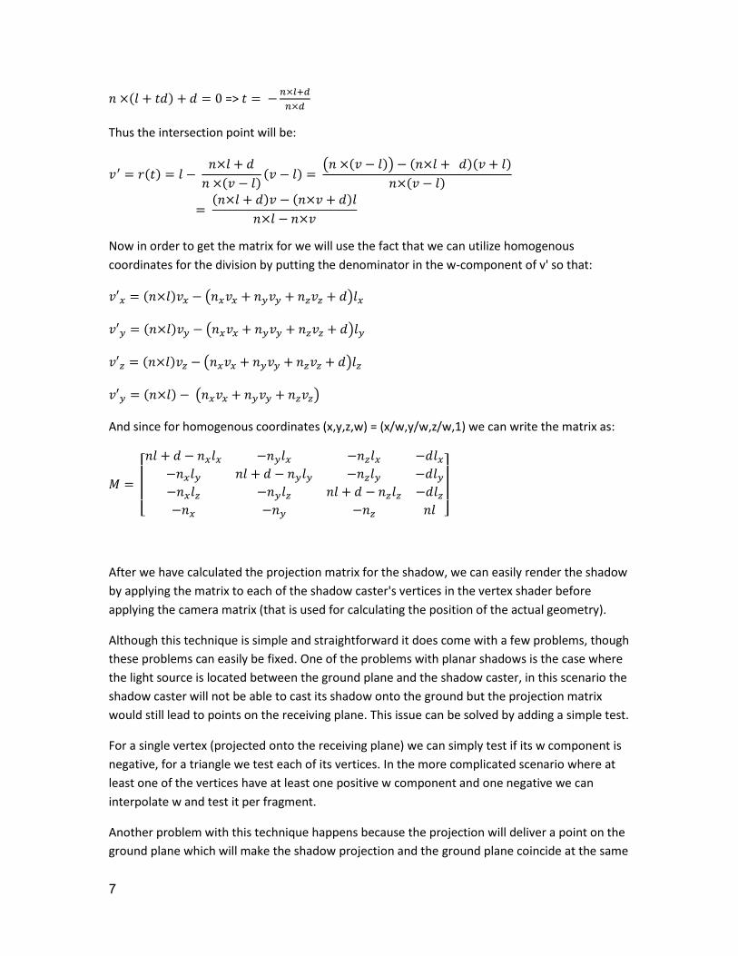
Figure 9: shadow acne.
The explanation to this issue is that if the shadow map had infinite resolution, the shadow
testing would be a matter of checking if the point is represented in the shadow map, however
with a discrete shadow map resolution, sampled points from the eye position are compared to
an image consisting of pixels, each of these pixel's value is defined by the world sample
corresponding to that pixel's center. When querying a view sample, it usually will not project
exactly to the same location as was sampled in the shadow map and therefore will be compared
to the average between nearest neighbors. This leads to problems when the view sample is
farther from the source than the corresponding value in the shadow map because unwanted
shadows can occur.
In order to deal with the shadow acne issue a threshold needs to be added in the form of a
depth bias that will offset the light samples slightly from the light source.
Although this might sound simple, it is in fact more problematic than it seems as the greater the
slope of the surface is the bigger the change in depth value between adjacent samples which
means that a larger value of depth bias is required in order to avoid the surface incorrectly
shadowing itself.
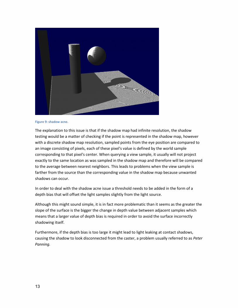
Furthermore, if the depth bias is too large it might lead to light leaking at contact shadows,
causing the shadow to look disconnected from the caster, a problem usually referred to as Peter
Panning.
14
Figure 10: Peter panning artifact.
The standard approach is to use two parameters for the bias, one constant and the other one
depends on the slope of the triangle as seen from the light source.
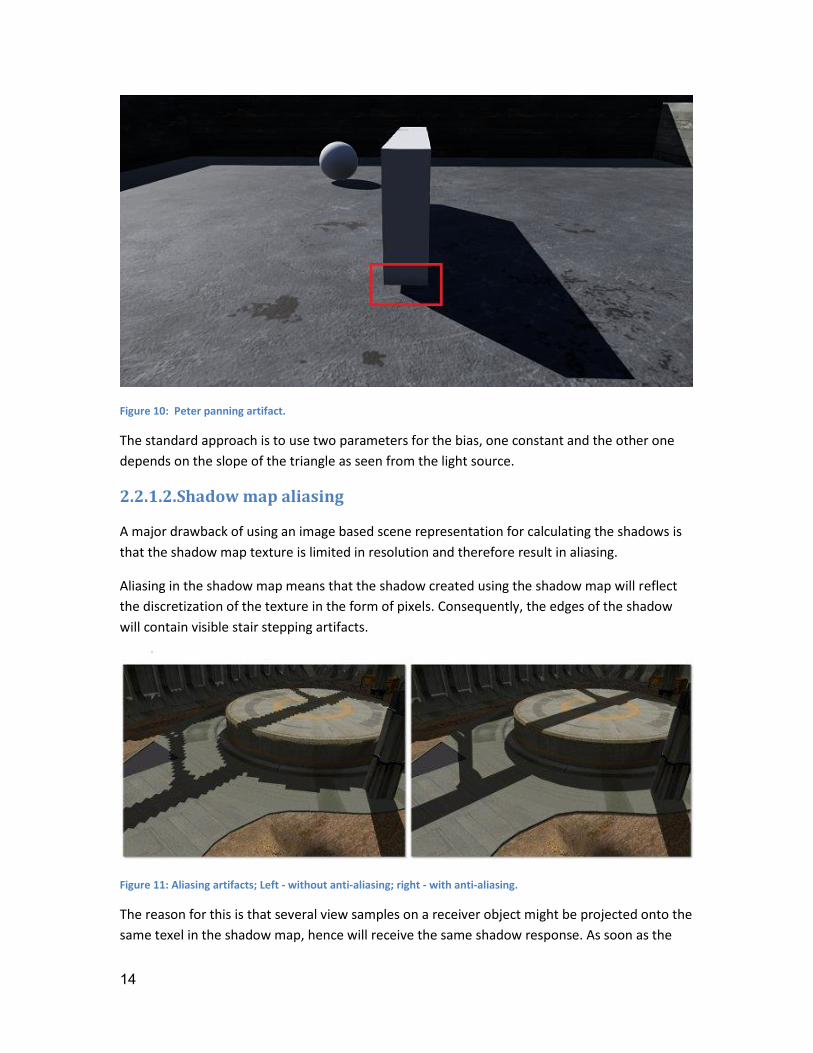
2.2.1.2.Shadow map aliasing
A major drawback of using an image based scene representation for calculating the shadows is
that the shadow map texture is limited in resolution and therefore result in aliasing.
Aliasing in the shadow map means that the shadow created using the shadow map will reflect
the discretization of the texture in the form of pixels. Consequently, the edges of the shadow
will contain visible stair stepping artifacts.
Figure 11: Aliasing artifacts; Left - without anti-aliasing; right - with anti-aliasing.
The reason for this is that several view samples on a receiver object might be projected onto the
same texel in the shadow map, hence will receive the same shadow response. As soon as the

15
object projects onto the next texel the shadow response might change drastically causing the
stair stepping artifacts mentioned above.
The best approach to dealing with these artifacts is to increase the shadow map resolution and
usually in modern games shadow map resolution exceeds the window size; 4096 and 8192 are
common choices. By using such large textures the chance of two view samples to fall into the
same texel is reduced.
Another solution is to create a shadow map per object and to adapt the shadow map resolution.
Although this solution is useful for creating high quality shadows it is considered more
complicated as it requires specialized scene structures and separated rendering passes.
Another common technique for dealing with aliasing in shadow maps is called "Percentage
Closer Filtering" or in short PCF. The basic principle of PCF is that instead of sampling one texel
in the shadow map in order to determine if a pixel is in shadow we also sample the texel's
neighbors and return a float in the range [0, 1] that reflects the weighted average of these
samples. We can use this result as the shadow factor for the pixel and by that makes the shadow
borders much smoother.
This technique is so common that a hardware implementation already exists in modern GPUs
and is also a base for a soft shadows technique I will describe later.
2.2.2.Omnidirectional shadows maps The technique that was presented in the previous section uses rendering for producing the
shadow map, therefore it is necessary to specify a light frustum which implies that the
technique is aiming at spot lights, which has a specific direction and a light radius.
What if we want to use the same technique to produce shadows from a point light?
The common way to deal with omnidirectional light sources is to create six light frustums
around the light source (each frustum represents a side in the cube that blocks that light source)
that together covers the entire sphere of directions.
According to [Wan07] a six-face spherical map can provide better utilization of resolution rather
than using a simple cube map, such a map can be thought of as a cube that is "inflated" to a
spherical shape such that each side of the map is a dome instead of flat.
Using six light frustums means that our scene's geometry has to be processed 6 times which
introduce a significant penalty in computation time.
Using Geometry shaders allows performing the required projection on a cube map in a single
pass but it doesn't prevent the geometry from being duplicated for each cube face.
It's worth mentioning that some techniques have been suggested to improve this method such
as using a parabolic map instead of a cube [Heidrich98] which enables the extraction of the

16
entire field with only two rendering passes, however cube maps remains the norm today due to
its simplicity.
2.3.Shadow volumes The shadow mapping technique we have seen in the previous section was based on an image
representation of the scene, which led to several problems caused by approximating the scene
in image space.
In this section we will introduce a different type of shadow technique that works directly in
object space thus does not suffer from the same problems as the previous technique did.
Instead of transforming our scene elements into a set of pixels our shadows will be described by
creating new geometric elements in our scene called shadow volumes (hence the name).
Since these volumes are being constructed accurately from the scene geometry it’s considered a
good method for creating accurate hard shadows, however this comes at an increased
computation cost.
The shadow volumes algorithm was first introduced by Frank Crow in 1977 [Crow77] and have
been evolving and maturing ever since, it was first named volumetric shadows, a name which
nowadays reserved for shadow algorithms that creates shadows in fog, clouds and smoke.
The basic concept in the shadow volume algorithm is that we extend our scene geometry in
order to create a new geometry that represents our shadows. For each triangle in our scene that
potentially cast a shadow on the scene we will define a shadow region, which will be define by
the triangle itself and by three quads that extends to infinity. Each of these quads is defined by
two of the triangle's vertices and by extruding these two vertices to infinity along the line from
the light source to the vertex.
Each of these quads along with the triangle itself form the triangle's shadow volume, the
triangle is usually referred to as the "near cap" as it adds a cap to the shadow volume.
We can now determine that a point lies in shadow if it is located within one or more of these
shadow volumes.

17
Figure 12: Shadow volumes technique.
Although the basic idea for this algorithm sounds rather simple, an efficient algorithm for this
technique is not so trivial to implement, thus requires a discussion about optimizing our
computation.
2.3.1.Naïve implementation The basic principle of the naïve approach is that each triangle in our occluder model will be
extended in the light's direction and will create a shadow volume, then when rendering the
shadow, all view samples will be tested against all shadow volumes (that is against each volume
that was produced earlier from each of the triangle that belongs to the occluder's model) in
order to determine if the sample is in shadow.
This method is not feasible for rendering complex scenes with where the number of polygons in
each model is high and high frame rate is critical (which is the case in video games and real time
simulations).
Although more efficient methods will be described later, I will give a brief explanation on how
the basic shadow volume can be created as this technique will also be useful in the more
advanced algorithms.
In order to extrude the shadow volumes to infinity, homogeneous coordinates can be used,
given a vertex in homogeneous coordinates, p:= ( 𝑝𝑥 , 𝑝𝑦, 𝑝𝑧, 1) we need to move it to infinity
along the line from the positional light l: = ( 𝑙𝑥 , 𝑙𝑦, 𝑙𝑧 , 1).
Using homogeneous coordinates, any point on a line between those two points can be
described by 𝛼𝑙 + 𝛽𝑝 with 𝛼, 𝛽 ∈ 𝑅. Consequently, the particular point 𝑝 − 𝑙 = (𝑝𝑥 − 𝑙𝑥, 𝑝𝑦 −
𝑙𝑦, 𝑝𝑧 − 𝑙𝑧, 0) lies on the line that corresponds to the direction into which the vertex should be
extruded. This point also lies in infinity since its w coordinate is 0. In order to create the
18
extruded shadow volume quad for an edge defined by two vertices v1, v2 we need to output the
vertices v1, v2, v1 - l, v2 – l. (the w-component will be equal to one for the first two vertices and
zero for the latter two that are extruded to infinity.
When using a directional light the process is even simpler as the two vertices at infinity are
located at the same position (and the quad becomes a triangle). The light itself describes the
direction into which the vertices should be extruded and these points simply become
( −𝑙𝑥 , −𝑙𝑦, −𝑙𝑧, 0).
The shadow volume quads should be oriented so that their plane equation have the interior of
the shadow volume on the inside and the exterior on the outside. In order to create a quad with
the right orientation we first need to figure out on which side of the triangle plane the light
source is located (which can be done using cross product).
2.3.2.Stencil Shadow Volumes It wasn't until 1991, with Heidmann's stencil shadows [Heidmann91] that shadow volumes
techniques became feasible for real-time dynamic scenes. The major benefit was that the
geometric computations (intersections and containment tests) were no longer used but instead,
we mapped to the existing z buffer and stencil buffer operations.
In order to simplify the explanation, we will assume that the eye position is located in light and
not shadow, we also make the assumption that the scene geometry is watertight (no holes) and
thus satisfies Jordan condition [Jordan87].
According to Jordan's theorem we can test whether a point lies inside or outside a shadow
volume by simply testing the number of intersections along the rays from the eye point to each
view sample, we count the number of times a ray enters versus exits a shadow volume, more
precisely we increase\decrease a counter every time the ray enters\exits a shadow volume.
Based on our previous assumption that the eye is located outside the shadow region, the final
count indicates the number of shadow volumes containing the view sample, a count different
than zero implies that the view sample lies in shadow.
Heidmann suggested to use a more GPU friendly computation than actually testing rays
explicitly against shadow volumes. Heidmann observed that a ray always enters a shadow
volume through a front facing polygon and leaves through a back facing polygon. Since each ray
is defined by a pixel in the image, one could implicitly test whether a ray enters a shadow
volume by simply drawing its front faces. All of the pixels that are covered by the drawn quad
will effectively enter the volume. Rendering all the back-facing quads will determine pixels
whose associated rays would leave the volume.
Heidmann suggested using the stencil buffer in order to implement these counters by rendering
all of the shadow volume quads and incrementing/decrementing the stencil values for front and
back facing polygons, since it represents entering/exiting shadow volumes.
19
In order to deal with shadow volumes that lie between the camera and the view sample
standard z-culling is used, where the depth buffer contains the shadow receiving scene, and any
updates to the z-buffer are disabled when rasterizing the quads. This way the stencil buffer will
contain the correct counter per pixel after having rendered all quads.
To summarize, the algorithm includes the following steps:
1. First pass – the scene is rendered from the viewport to create the z-buffer and the
ambient lighting will also be calculated in this step and saved to a second buffer.
2. Second pass – in this step the z-buffer and color buffer writing is disabled and we render
all front facing shadow volume quads to the stencil buffer. Only when a shadow volume
quad passes the depth test the counter in the stencil buffer is incremented. In the next
step, all back facing shadow volume quads are rendering, this time decrementing the
stencil buffer for quads that passes the depth test.
3. Third pass – in the final pass, the scene is rendered again, this time adding the specular
and diffuse lighting contribution into the color buffer while using the stencil buffer from
the previous stage as a mask to discard any pixel in shadow.
This type of stencil updates presented here are usually referred to as "z-pass algorithm" and it’s
a much more efficient and practical approach than the naïve implementation presented earlier.
However, there are several basic improvements that can be made and also there's a need to
address the assumptions we made earlier about the location of the eye (see z-fail algorithm
[Bilodeau99] or Carmack's reverse [Carmack00]) and the scene being watertight. But these
topics are beyond the scope of these summary and can be explored more thoroughly in the
sources and articles found in the reference section.
2.3.3.Silhouette-Based Shadow Volumes For watertight models, a good optimization technique one can use, is to omit the inner quads of
the shadow volume as these does not contribute to determine whether a point lies in shadow or
light. Instead of using all of the model's edges to create the shadow volumes, a different
approach can be taken. The shadow volume can be built using only the model's silhouette edges
as seen from the light, these edges will be extruded in the lights direction to create the shadow
volume. The silhouette edges can be found by searching for shared edges between one triangle
that is front facing and one triangle that is back facing the light source.
2.3.4.Level of Details Another possible technique that can be used in order to increase performance is to use a
simpler approximation to the model, one which contains less polygons so that the volumes can
be generated fast. This also opens up the possibility of using different LOD objects for shadow
volumes depending on the model's distance from the camera. E.g. use a simpler model when
the object is far and use a complex model when the object is near the viewer's eye.

20
3.Soft shadows techniques As mentioned earlier, soft shadows are important to achieve high realism in scenes and are the
result of using an area light (which has a clear size and shape as opposed to a point light that has
no size).
Figure 13: Hard shadows vs. soft shadows.
In this section I will give a brief introduction to how soft shadows can be created and describe
briefly some of the most common techniques used today. Soft shadows techniques are divided
into two types of algorithms, ones that are based on an image-based approach and are built
upon the shadow mapping algorithm and ones that are based on an object-based approach and
are built upon the shadow volume algorithm.
3.1.Image based approach Shadow mapping is the most used technique used today to create shadows it is also the most
active on shadow researching in the last years, unfortunately the standard shadow mapping
algorithm is unable to generate shadows with penumbra as it cannot handle area lights,
therefore shadow mapping needs to be extended in order to support the creation of soft
shadows, and as we will see in this section most of the common soft shadows techniques are an
extension of the shadow mapping algorithm.
3.1.1.Combination of several point based shadow images The simplest image based technique used to create soft shadow maps is to use several sample
points to simulate the area light. Each of these sample points will used to create a shadow map
(a binary occlusion map), additive blending will be used to accumulate the contribution of each
light and the softness of the shadow will be determined by the number of sample points used.
The biggest advantage of this method is that it simple to implement and can achieve good
results and when enough samples are used the shadow will contain more information that
shadows achieved with other image based technique thus will appear to be more physically
accurate.
21
The drawback of using this method is that this method is relatively slow as the rendering time
will increase linearly with the number of samples used to approximate the area light and when
too few samples are used unwanted artifacts will be introduced.
3.1.2.Fixed sized penumbra filtering techniques The following techniques can be used to blur the shadow in order to a soft-shadow-life
appearance, the results these techniques can achieve are pretty good but the drawback is that
the resulting penumbra is fixed sized thus does not reflect the occluding object's distance from
the shadow receiving object.
PCF (Percentage Closer Filtering) – We mentioned PCF earlier as a technique to handle
shadow map aliasing, this technique is also commonly used to create a fixed sized
penumbra soft shadows
VSM (Variance Shadow Maps) – Introduced by Donnelly and Lauritzen [Donnelly06], this
technique uses statistics to facilitate precomputation of shadow-map filtering. The basic
idea of this technique is to replace the standard shadow map query with an analysis of
the distribution of depth values and employs variance and Chebyshev’s inequality to
determine the amount of shadowing over an arbitrary filter kernel thus allowing the
shadow maps to be pre-filtered and create very fast soft shadows with large filter
kernels.
CSM (Convolution Shadow Maps) – Introduced in [Annen07] and is the first approach
that allows filter precomputation based on a linear signal theory framework by using
Fourier expansion to derive suitable basis functions for the approximations of the
shadow comparison function.
ESM (Exponential Shadow Maps) – Introduced in [Annen08b] and [Salvi08], this
technique is based on the CSM technique but instead of using Fourier expansion it uses
simple exponential which voids much of the storage requirements that the CSM method
has.
3.1.3.Variable sized penumbra filtering techniques The following techniques are different than the ones mentioned before as they take into
account the distance between the object and therefore the penumbra width is of variable size.
PCSS (Percentage Closer Soft Shadows) – one of the most common techniques for image
based soft shadows, this technique is based on the PCF technique and will be discussed
in details later.
PCSS + VSM\CSM – a combination of the PCSS technique with either VSM or CSM
techniques mentioned in the previous section.
Backprojection – refers to a group of algorithms initially introduced in [Atty06], the basic
idea in these techniques is to obtain a shadow map from the light source's center and
reconstruct potential occluders in world space from it. These occluders are then back-
projected from the currently considered receiver point p onto the light's plane to
estimate the visible fraction of the light area. These techniques mainly differ in the type
of occluder approximation that is employed, the way the computation is organized and

22
how the occluded light area is derived. These choices influence the performance of the
technique, its generality, robustness and visual quality.
3.1.3.1.PCSS explained
The basic idea of the PCSS technique is to calculate the penumbra width and use it when
filtering the shadow map to achieve soft shadows. There are 3 parts in this technique:
Blocker search – first we need to calculate the shadow region 𝑅𝑆 that contains samples of
the relevant occluders. The shadow region is defined by the intersection of the light-
receiver-point pyramid (where the light source is the base and the point p is the apex) with
the shadow-map's near plane, the region is then searched for blockers which are simply
identified by performing a standard shadow map test, meaning all shadow map entries that
are closer to the light source than p are considered as blockers.
Figure 14: Illustration of the blocker search step.
Penumbra-width estimation – in the second part of the algorithm we need to calculate the
penumbra width, we make the simplifying assumption that there is only one occluder that is
furthermore planar and parallel to the area light's plane. For this plane, we use the average
depth of all the blockers that we found in the blocker search phase, we mark it with 𝑍𝑎𝑣𝑔.
We also make the assumption that point p belongs to a planar receiver that is also parallel
to the planar occluder, the penumbra width is then calculated using the formula:
𝑊𝑝𝑒𝑛𝑢𝑚𝑏𝑟𝑎 = 𝑝𝑧 − 𝑧𝑎𝑣𝑔
𝑧𝑎𝑣𝑔𝑤𝑙𝑖𝑔ℎ𝑡
Filtering – now that we have the penumbra width we can use it to derive a suitable PCF
window by projecting the penumbra width onto the shadow-map's near plane using the
equation:
𝑤𝑓 = 𝑧𝑛𝑒𝑎𝑟
𝑝𝑧𝑤𝑝𝑒𝑛𝑢𝑚𝑏𝑟𝑎
After that the shadow map can be queried and filtered according to the window size.
3.2.Geometry based approach Although Geometry based algorithms for soft shadows are less commonly used and less
researched than the shadow mapping based algorithms when considering a shadowing

23
technique one should also consider one of the following geometry based algorithms (based on
the shadow volume technique introduced earlier:
Using several point samples to simulate an area light – same as with shadow mapping,
one can use multiple sampling points to generate shadow volumes and combine them
into a soft shadow using additive blending.
Soft shadow volumes – The idea of this methods is the concept of using "Penumbra
wedges" [Akenine-Moller02, Assarsson04]. The basic idea behind this technique is to
encapsulate the penumbra regions by geometrically creating a wedge from each
silhouette edge, where the wedge encloses the penumbra cast by the corresponding
edge. Shadow-receiving points that lie inside the penumbra wedge receive a shadow
value based on interpolation between the inner and outer wedge borders. Borders are
not allowed to overlap otherwise artifacts will appear (Although a later technique
suggested in [Assarsson03a] suggest a way to remove this limitation).
The benefit of using these types of techniques is that the resulting shadow is very
pleasing and does not suffer from discretization artifacts or undesirable discontinuities.

24
4.Conclusion and further reading Although real-time shadow computation is not an easy task we've seen several basic techniques
that are not too difficult to implement and can achieve very nice results. We've also seen a few
more advanced techniques that will allow us to solve some of the problems encountered in the
more simpler techniques such as aliasing issues and the need for soft shadows. Shadow
techniques are still actively researched around the world and new techniques and algorithms
that allows to achieve more accurate shadows in a shorter time keep emerging and will keep
improving as hardware becomes better and faster and games that strive for realism will require
better techniques.
There are many topics relating to shadow techniques that I haven't touched in this summary, for
further reading I suggest going through some of the material and articles in the references
section.
25
5.References Real time shadows 1st edition by Elmar Eisemann, Michael Schwarz, Ulf Assarsson,
Michael Wimmer, CRC Press 2011.
A survey of Real-Time Soft Shadows Algorithms, Jean-Marc Hasenfratz, Marc
Lapierre, ,Computer Graphics Forum, Volume 22, Number 4, page 753--774 - dec 2003
Variance Shadow Mapping by Kevin Myers, Nvidia January 2007
SIGGRAPH 2013 soft shadows course
Shadow Mapping and Shadow Volumes: Recent Developments in Real-Time,Shadow Rendering, University of British Columbia, CS514 Advanced Computer Graphics: Image Based Rendering, Instructor: Wolfgang Heidrich, Project Report, Andrew V. Nealen, Technische Universit¨at Darmstadt
Percentage-Closer Soft Shadows, Randima Fernando, NVIDIA Corporation
Real-time Soft Shadows in a Game Engine, Kasper Fauerby, Carsten Kjær, 14th December 2003
Real-Time Shadows, Eric Haines [email protected], Tomas M¨ oller [email protected], [Excerpted and updated from the book ”Real-Time Rendering”, by Tomas M¨ oller and Eric. Haines, A.K. Peters, ISBN 1568811012. See http://www.realtimerendering.com/]
Penumbra Maps: Approximate Soft Shadows in Real-Time, Chris Wyman and Charles Hansen, School of Computing, University of Utah, Salt Lake City, Utah, USA
Fast, Practical and Robust Shadows, Morgan McGuire, John F. Hughes, and Kevin T. Egan, Brown University, Mark J. Kilgard and Cass Everitt, NVIDIA Corporation
http://roar11.com/2015/05/dealing-with-shadow-map-artifacts/
http://www.zachlynn.com/
http://www.peachpit.com/articles/article.aspx?p=486505&seqNum=6
[Akenine-Moller02] Akenine-Moller, T. and Assarsson, U. 2002. Approximate soft
shadows on arbitrary surfaces using penumbra wedges. In proceedings of Eurographics
Workshop on Rendering 2002, pp. 161-166.
[Annen07] Annen, T., Mertens, T., Bekaert, P., Seidel, H.-P., and Kautz, J. 2007
Convolution shadow maps. In Proceedings of Eurographics Symposium on Rendering
2007, pp. 51-60.
[Annen08b] Annen, T., Mertens, T., Seidel, H.-P, Flerackers, E., and Kautz, J. 2008.
Exponential Shadow maps. In Proceedings of Graphics interface 2008, pp. 155-161.
[Atty06] Atty , L. Holzschuch, N., Lapierre, M., Hasenfratz, J.-M., Hansen, C., and Sillion,
F. X. 2006. Soft shadow maps: Efficient sampling of light source visibility. Computer
Graphics Forum, 25,4, 725-741.

26
[Assarsson03a] Assarsson, U. and Akenine-Moller, T. 2003. A geometry-based soft
shadow volume algorithm using graphics hardware. ACM Transactions on Graphics, 22,
3 (Proceedings of ACM SIGGRAPH 2003), 511-520.
[Assarsson04] Assarson, U. and Akenine-Moller, T. 2004.Occlusion culling and z-
fail for soft shadow volume algorithms. The visual compter, 20, 8-9.
[Bilodeau99] Bilodeu, W. and Songy, M. 1999. Real time shadows. Creativity 1999,
Creative Labs Inc. Sponsored game developer conferences, Los Angeles, California, and
Surrey, England.
[Carmack00] Carmack, J. 2000. Z-fail shadow volumes. Internet Forum.
[Crow77] Crow, F.C. 1977. Shadow algorithms for computer graphics. Computer
Graphics, 11, 2 (Proceeding of ACM SIGGRAPH 77), 242-248.
[Donnelly06] Donnelly, W. and Laurizen, A. 2006. Variance shadow maps. In Proceedings
of ACM SIGGRAPH symposium on Interactive 3D Graphics and Games 2006, pp. 161-165.
[Heidmann91] Heidmann, T. 1991. Real shadows real time. IRIS Universe, 18, 28-31.
[Jordan87] Jordan, C. 1887. Cours d'analyse. L'Ecole Polytechnique, pp. 587-594.
Available online at: http://maths.ed.ac.uk/~aar/jordan/jordan.pdf .
[Salvi08] Salvi, M. 2008. Rendering filtered shadows with exponential shadow
maps. In ShaderX6: Advanced Rendering Techniques (edited by W. Engel), pp.
257-274. Charles River Mdia, Hingham, MA. ISBN 978-1-58450-544-0.
[Williams78] Williams, L. 1978. Casting curved shadows on curved surfaces. Computer
Graphics, 12,3 (Proceedings of ACM SIGGRAPH 78),270-274.
[Wan07] Wan, L., Wong, T.-T., and Leung, C,-S. 2007, Isocube: Exploiting the cubemap
hardware. IEEE Transactions on Visualization and Computer Graphics, 13, 4, 720-731.