shadow - marriesadvancedgraphics.marries.nl/lectures/03_shadows.pdf · variance shadow maps use...

Advanced Graphics 2012-2013 Advanced Graphics 2012-2013

Advanced Graphics

Shadow

Shadow

Advanced Graphics 2012-2013

Shadow

Important for depth perception

Shadow 2


Overview

Recap of basic techniques Various problems

– Filtering – Varying penumbra – Light source types

• Point light source • Directional light source

– Volumetric shadow – Subsurface scattering

Shadow 3


Shadow Volumes

Shadow volumes

– Rarely used anymore

– Extrude geometry

– Use stencil buffer to mark shadowed areas

Shadow 4


Shadow Volumes

Creates extremely sharp shadows – Usually not preferred

Bad worst-case performance – Why?

• Extreme overdraw

Shadow 5


Shadow Maps

Render scene depth from light source

– Store in shadow map

– Compare distancez from light source with shadow map depth

Shadow

Unshadowed: Shadow map depth == distancez(point, light)

Shadowed: Shadow map depth < distancez(point, light)

6


Shadow Maps

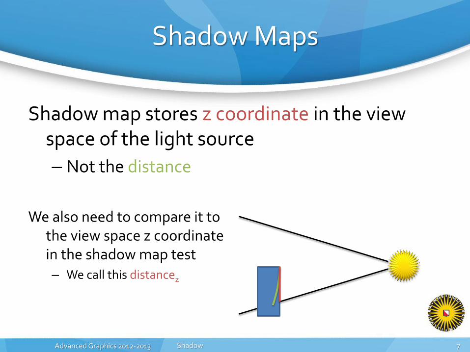
Shadow map stores z coordinate in the view space of the light source

– Not the distance

We also need to compare it to the view space z coordinate in the shadow map test – We call this distancez

Shadow 7


Shadow Maps

Shadow 8


Shadow Acne

Shadow map has a finite resolution

– Discretization artifacts

Shadow 9


Shadow Acne

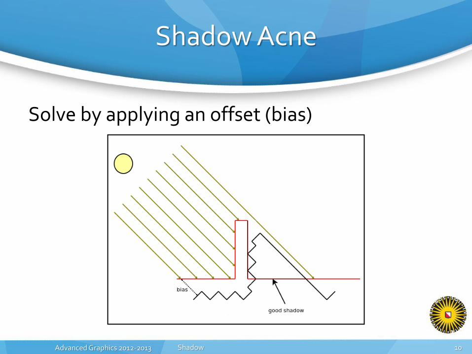
Solve by applying an offset (bias)

Shadow 10


Shadow Acne

Hard to pick a bias for every situation

Too much bias can cause “Peter Panning”

– Because everything seems to float

Shadow 11


FILTERING Shadow

Filtering

Varying penumbra

Light source types

Volumetric shadow

Subsurface scattering


Aliasing

Shadow map resolution must be high

– To prevent aliasing

– Can we interpolate the shadow map?

Shadow 13


What happens when we interpolate the shadow map? – We want the result to be half-shadowed – But it is fully shadowed

Shadow test is

– distancez > average(shadowmap)

But it should be – average(distancez > shadowmap)

Shadow Map Interpolation

Shadow 14


Percentage Closer Filtering

Percentage Closer Filtering (PCF)

– Execute the shadow test multiple times

• average(distancez > shadowmap)

Hardware supported in DX10+

– HLSL SampleCmp function (instead of Sample)

Shadow 15



Shadow boundary is still blocky – Increase filter radius

Shadow 16


Increasing the filter radius requires a lot of samples

– Need 64 samples in this case

– Bandwidth bottleneck


Shadow

2x2 samples 4x4 samples 8x8 samples

17



Randomize the sample locations

– Less samples

– Introduces noise

Shadow 18


Pre-Filtering

Sample from a downscaled shadow map – Do the filtering (averaging) in advance

• Create mipmaps

– But we (still) can’t use the interpolated values

Shadow 19

Mipmaps:

Magnified:


Variance Shadow Maps

Stores a depth description which can be filtered – Based on probability theory

A shadow map is not probabilistic – But it does have a distribution

The variance describes the width of the distribution

Shadow 20


𝜇-𝜎 𝜇 𝜇+𝜎

Distributions – Mean 𝜇 = 𝐸 𝑥 (expected value) – Variance 𝜎2 = 𝐸 𝑥2 − 𝐸 𝑥 2 – First moment 𝑀1 = 𝐸 𝑥 – Second moment 𝑀2 = 𝐸 𝑥2


Shadow 21



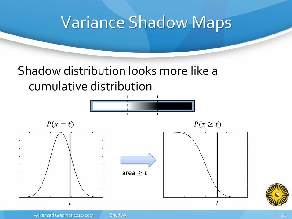
Shadow distribution looks more like a cumulative distribution

Shadow

area ≥ 𝑡

𝑃(𝑥 = 𝑡) 𝑃(𝑥 ≥ 𝑡)

22

𝑡 𝑡



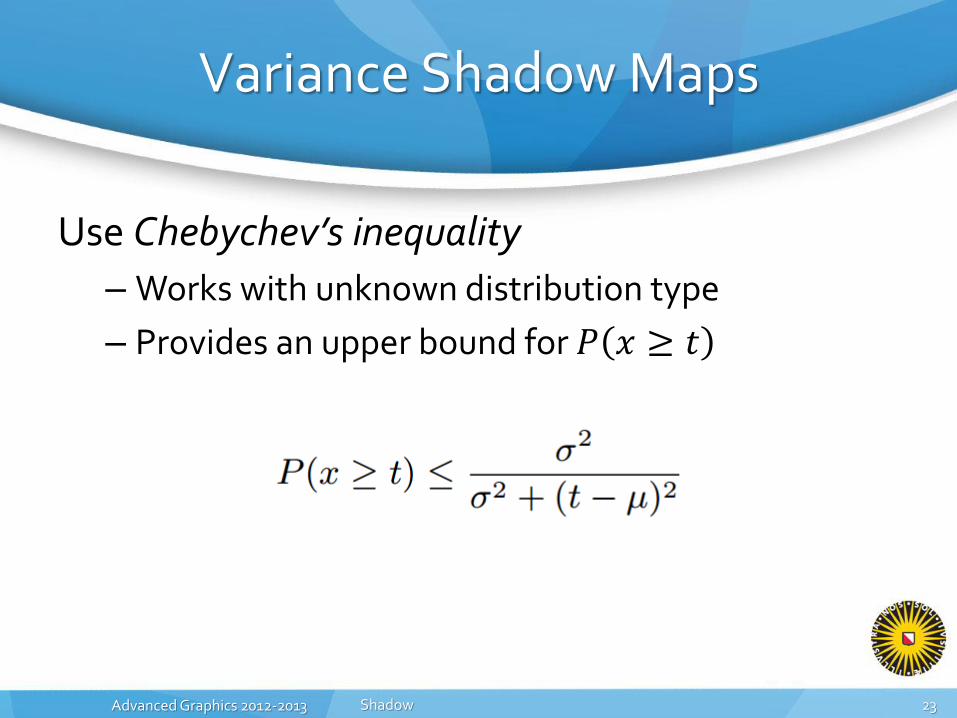
Use Chebychev’s inequality

– Works with unknown distribution type

– Provides an upper bound for 𝑃 𝑥 ≥ 𝑡

Shadow 23



In this context

– 𝑃 𝑥 ≥ 𝑡 is the fraction this position is lit

– 𝑡 is the distancez from this position to the light source

– 𝜇 and 𝜎2 describe the shadow map depth distribution

• Calculated using 𝐸 𝑥 and 𝐸 𝑥2 , where 𝑥 is the depth value

Shadow 24

We store the depth value 𝑥 and the squared depth value 𝑥2 – Interpolation averages the depth, giving 𝐸 𝑥 and 𝐸 𝑥2


Example

– Interpolate 𝑀1 and 𝑀2 – Calculate 𝜇 and 𝜎2 – Calculate 𝑃 𝑥 ≥ 𝑡

Shadow

depth = 0.5

depth = 0.6

𝑀1 = 0.5 𝑀2 = 0.25

𝑀1 = 0.6 𝑀2 = 0.36

𝜇 = 𝐸 𝑥

𝜎2 = 𝐸 𝑥2 − 𝐸 𝑥 2

𝑀1 = 𝐸 𝑥

𝑀2 = 𝐸 𝑥2

𝜇

𝜎2 𝑃 𝑥 ≥ 𝑡

25


Proof

Proof for this simple case:

Shadow

𝑝 is the interpolation parameter 𝑑1 and 𝑑2 are the depths

26



Works for all kinds of linear filtering – Linear interpolation

– Mipmaps

– Blurring

We only need to store 𝑀1 and 𝑀2 (depth and depth2)

Shadow 27



One major disadvantage

– Can cause light bleeding

Shadow 28


Light Bleeding

Back to our example

– Investigate what happens when we vary the sampling depth 𝑡

Shadow

depth = 0.5

depth = 0.6

𝑀1 = 0.5 𝑀2 = 0.25

𝑀1 = 0.6 𝑀2 = 0.36

𝜇 = 𝐸 𝑥

𝜎2 = 𝐸 𝑥2 − 𝐸 𝑥 2

𝑀1 = 𝐸 𝑥

𝑀2 = 𝐸 𝑥2

1

0.55 0.6

29


Light Bleeding

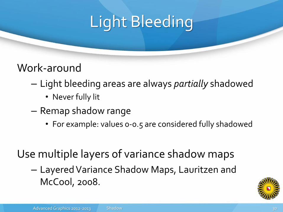
Work-around

– Light bleeding areas are always partially shadowed

• Never fully lit

– Remap shadow range

• For example: values 0-0.5 are considered fully shadowed

Use multiple layers of variance shadow maps

– Layered Variance Shadow Maps, Lauritzen and McCool, 2008.

Shadow 30


Numerical Stability

Variance calculation subtracts two large values – 𝜎2 = 𝐸 𝑥2 − 𝐸 𝑥 2 – The result (variance) is fairly small

• But important for our calculations

Catastrophic cancellation – Floats cannot retain small fractions for large values

• 1.0000000001 − 1 = 0

Floats (32 bit) are good enough in this case – But half floats (16 bit) can cause artifacts

Shadow 31



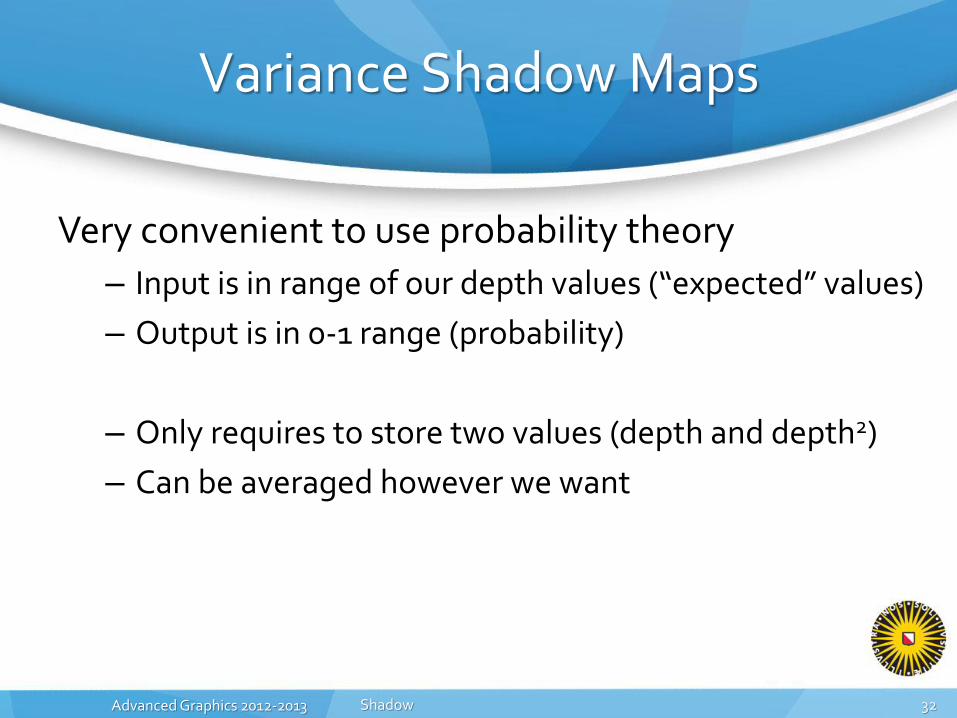
Very convenient to use probability theory

– Input is in range of our depth values (“expected” values)

– Output is in 0-1 range (probability)

– Only requires to store two values (depth and depth2)

– Can be averaged however we want

Shadow 32


VARYING PENUMBRA Shadow

Filtering

Varying penumbra

Light source types

Volumetric shadow



Umbra

Penumbra

Caused by area light sources

Shadow 34

Penumbra


Penumbra

Larger depending on the distance to occluder

Shadow

Hard Soft Correct

35


Percentage Closer Soft Shadows

Vary shadow softness depending on penumbra width Approximate penumbra width

– Assumes parallel light source, occluder and receiver

Shadow 36

𝑤𝑝𝑒𝑛𝑢𝑚𝑏𝑟𝑎 =𝑑𝑟𝑒𝑐𝑒𝑖𝑣𝑒𝑟 − 𝑑𝑜𝑐𝑐𝑙𝑢𝑑𝑒𝑟

𝑑𝑜𝑐𝑐𝑙𝑢𝑑𝑒𝑟∙ 𝑤𝑙𝑖𝑔ℎ𝑡 𝑠𝑜𝑢𝑟𝑐𝑒

𝑤𝑙𝑖𝑔ℎ𝑡 𝑠𝑜𝑢𝑟𝑐𝑒

𝑤𝑝𝑒𝑛𝑢𝑚𝑏𝑟𝑎

𝑑𝑜𝑐𝑐𝑙𝑢𝑑𝑒𝑟

𝑑𝑟𝑒𝑐𝑒𝑖𝑣𝑒𝑟 − 𝑑𝑜𝑐𝑐𝑙𝑢𝑑𝑒𝑟



Known variables

– 𝑑𝑟𝑒𝑐𝑒𝑖𝑣𝑒𝑟

– 𝑤𝑙𝑖𝑔ℎ𝑡 𝑠𝑜𝑢𝑟𝑐𝑒

Unknown variables

– 𝑑𝑜𝑐𝑐𝑙𝑢𝑑𝑒𝑟 • Read from the shadow map, but where?

Shadow 37





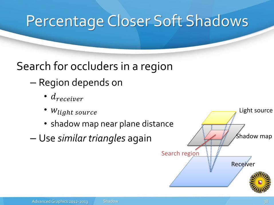
Search for occluders in a region

– Region depends on

• 𝑑𝑟𝑒𝑐𝑒𝑖𝑣𝑒𝑟

• 𝑤𝑙𝑖𝑔ℎ𝑡 𝑠𝑜𝑢𝑟𝑐𝑒

• shadow map near plane distance

– Use similar triangles again

Shadow 38

Light source

Shadow map

Receiver

Search region



Calculate 𝑑𝑜𝑐𝑐𝑙𝑢𝑑𝑒𝑟 by averaging the occluder depths

Search region can be relatively large – Semi-random sampling

• Still needs a lot of samples (at least 16)

– Can we use pre-filtering? • No, we need the average of the occluder depth (not the

average of all depths)

Shadow 39


Select Shadow Softness

Occluder depth is known

– Calculate 𝑤𝑝𝑒𝑛𝑢𝑚𝑏𝑟𝑎

– Next step: select shadow softness

Select filter width based on 𝑤𝑝𝑒𝑛𝑢𝑚𝑏𝑟𝑎

Shadow 40





For variance shadow maps – Use filter width size to select a mip-level – Interpolate between nearby values in the

mip-level

Shadow 41


Mipmapping

Lower resolution versions of the same texture

– Contains averaged values

– Easy to retrieve the average of a large surface

• With much less samples

Shadow 42

Mipmaps:

Magnified:



For variance shadow maps – Use filter width size to select a mip-level – Interpolate between nearby values in the

mip-level

However, this is just linear interpolation – Visible as boxy artifacts

We need better filtering

– The exact average of a certain region

Shadow 43


Summed-Area Table

Contains the sum of everything to the top-left

Allows us to retrieve the sum of an arbitrary rectangle

Shadow 44

2 1 3 1

4 0 1 2

2 2 1 0

0 3 4 3

2 3 6 7

6 7 11 14

8 11 16 19

8 14 23 29

Original

Summed-area table

2 1 3 1

4 0 1 2

2 2 1 0

0 3 4 3

2 3 6 7

6 7 11 14

8 11 16 19

8 14 23 29

= -

2 3 6 7

6 7 11 14

8 11 16 19

8 14 23 29


Summed-Area Table

Generating the SAT on the GPU – Similar to the sum example from lecture 1

For the 1D case (prefix sum):

More efficient methods available [Blelloch 1990]

Shadow 45

1 2 3 4 5 6 7 8



The summed-area table gives the sum

– Divide by the area for the average

Combination is called Summed-Area Variance Shadow Maps (SAVSM)

– When used with PCSS:

Shadow 46


LIGHT SOURCE TYPES Shadow

Filtering

Varying penumbra

Light source types

Volumetric shadow



Spotlight

Shadow maps can be used directly for spotlights

Shadow

Shadow map


Point Light

But what about (omnidirectional) point lights?

– Where do we place the shadow map?

Shadow 49

?


Point Light

Use 6 shadow maps

– Each with a 90o field-of-view

– Store in a cubemap

Shadow 50


Point Light

Not very efficient – Can render to all faces simultaneous using geometry

shader • Is this faster? • Usually not in practice

– Can use dual paraboloid mapping

Shadow 51


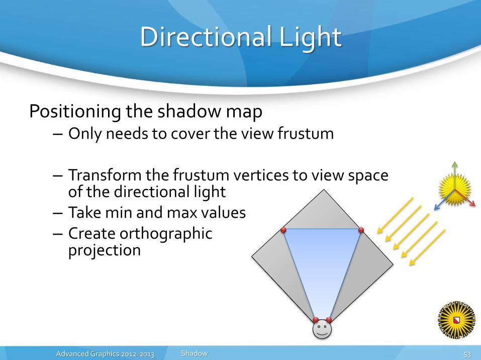
Directional Light

Lights everything from the same direction

– Orthographic projection

– How to position the shadow map?

• Needs to cover everything visible

Shadow 52


Directional Light

Positioning the shadow map – Only needs to cover the view frustum

– Transform the frustum vertices to view space

of the directional light – Take min and max values – Create orthographic

projection

Shadow 53


Directional Light

Poor shadow map usage

– Wasted space

– Accuracy independent of camera distance

Shadow 54


Perspective Shadow Maps

Can we warp the shadow map? – Re-use the wasted space for nearby accuracy

Render the shadow map in Normalized Device Coordinate space – Directional light becomes an (inverted) point light!

Shadow 55


Perspective Shadow Maps

Can give good shadow quality

– Quality is highly view-dependent

– Many bad cases

• Occluders behind near plane

• Bad precision when view direction aligns with light direction

– Hard to get right for every case

Shadow 56

warp


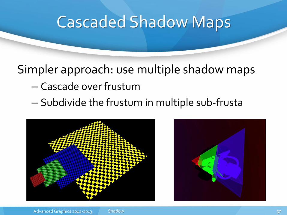
Cascaded Shadow Maps

Simpler approach: use multiple shadow maps

– Cascade over frustum

– Subdivide the frustum in multiple sub-frusta

Shadow 57



Movement causes shadow edges to shimmer

Shadow 58



Snap shadow map to grid

– Only move whole pixels

– Needs additional space

• Grid cannot rotate

– Good solution

Does not solve shimmering when moving the light source

Shadow 59


VOLUMETRIC SHADOW Shadow 60

Filtering

Varying penumbra

Light source types

Volumetric shadow



Translucent Volumes

Uniform unbounded volumes

– Fog

Non-uniform bounded volumes

– Smoke/clouds

Shadow 61


Rendering Translucent Volumes

Translucency accumulates along the view ray

Shadow 62




– Directional light source

– Lighting is equal at every point

• Simple function of depth

Shadow 63




– Point light source

– Lighting varies

• How can we solve this?

Shadow 64



Keep it simple (for this lecture)

– Discretize the function

– Volume ray marching

• Sampling along the ray

• Blend the results

Shadow 65



Non-uniform bounded volumes

– For all light source types

– Use ray marching

• Sample translucency from 3D texture (for example)

Shadow 66


Volumetric Shadow

Volume being shadowed

Self-shadow of the volume

Volume affecting the environment

– Partial shadow

Shadow 67


Volumetric Shadow

General approach

– Test shadow for each ray march point

Shadow 68


Volumetric Shadow

Volume being shadowed – Most relevant for uniform unbounded shadows

– Use regular shadow map to test for shadow

Effect called crepuscular rays or god rays

Shadow 69


Volumetric Shadow

Volume being shadowed

Self-shadow of the volume

Volume affecting the environment

– Partial shadow

Shadow 70


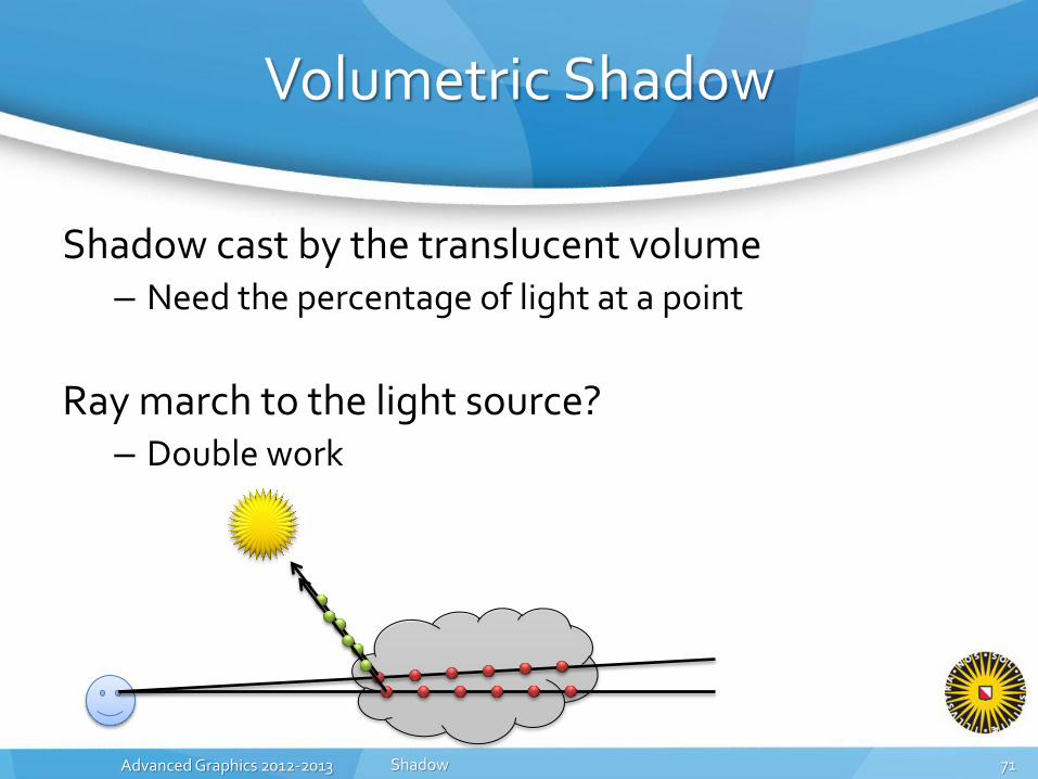
Volumetric Shadow

Shadow cast by the translucent volume – Need the percentage of light at a point

Ray march to the light source? – Double work

Shadow 71


Deep Shadow Maps

Store opacity as a piecewise linear function – Simplify to reduce storage

Can sample percentage of light at each point – Extremely slow

Shadow 72


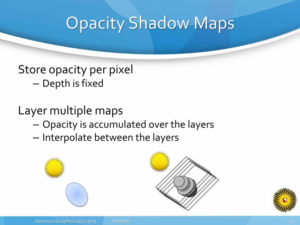
Opacity Shadow Maps

Store opacity per pixel – Depth is fixed

Layer multiple maps – Opacity is accumulated over the layers – Interpolate between the layers

Shadow 73


Hair shadows

Uses volumetric shadow

– Hairs are too small for regular shadow maps

Shadow 74


SUBSURFACE SCATTERING Shadow 75

Filtering

Varying penumbra

Light source types

Volumetric shadow



Subsurface Scattering

Volumetric rendering was single bounce

– Actually simplification

Shadow



Subsurface scattering occurs with multiple bounces

– Diffuses the light

Shadow 77



Can be observed in dense translucent materials

– For example: milk, marble, skin

Shadow 78



Problem can be very complex

– Especially for multi-layered materials (e.g. skin)

Shadow 79



Approximate effects on macro scale

– Partial translucency

– Diffusion

Shadow 80


Partial Translucency

Light decreases with distance travelled through the material – Use shadow map to calculate entrance depth

– Subtract from exit depth

Shadow 81


Diffusion

Diffuse (blur) the light over the surface – Only the light, not the color

– What to blur? • Light image rendered from the light source?

• Light image rendered from the camera?

Shadow 82


Texture-Space Diffusion

Perform the blur in texture-space – Tangent space with uv-mapping

Calculate lighting on a texture – Blur the lighting texture

Shadow 83



Rendering the lighting to a texture – Requires mindset switch

Render the model – But use the UV-coordinate as vertex position – The world position is used to calculate the lighting

Shadow 84



Blur the light texture

– Special blur kernel to simulate diffusion properties

• Depends on material

Requires a perfect UV-mapping • Impossible

• Correct for over/under stretching

• Correct for seams

Shadow 85


CONCLUSION Shadow 86

Filtering

Varying penumbra

Light source types

Volumetric shadow



Conclusion

Many different shadow techniques

– A lot can be combined

Cascaded Perspective Summed-Area Variance Shadow Maps with Percentage Closer Soft Shadows?

– No problem!

– CPSAVSM+PCSS

Shadow 87

shadow - marriesadvancedgraphics.marries.nl/lectures/03_shadows.pdf · variance shadow maps use...

Documents