sgn-2506: introduction to pattern recognitionjupeto/jht_lectnotes_eng.pdf · sgn-2506: introduction...
TRANSCRIPT

SGN-2506: Introduction to Pattern Recognition
Jussi TohkaTampere University of TechnologyDepartment of Signal Processing
2006 - 2008
March 12, 2013

ii
Preface
This is an English translation of the lecture notes written originally in Finnish forthe course SGN-2500 Johdatus hahmontunnistukseen. The basis for the originallecture notes was the course Introduction to Pattern Recognition that I lectured atthe Tampere University of Technology during 2003 and 2004. Especially, the coursein the fall semester of 2003 was based on the book Pattern Classification, 2nd Editionby Richard Duda, Peter Hart and David Stork. The course has thereafter divertedfrom the book, but still the order of topics during the course is much the same asin the book by Duda et al.
These lecture notes correspond to a four credit point course, which has typicallybeen lectured during 24 lecture-hours. The driving idea behind these lecture notesis that the basic material is presented thoroughly. Some additonal information arethen presented in a more relaxed manner, for example, if the formal treatment ofa topic would require too much mathematical background. The aim is to providea student with a basic understanding of the foundations of the statistical patternrecognition and a basis for advanced pattern recognition courses. This necessarilymeans that the weight is on the probabilistic foundations of pattern recognition,and specific pattern recognition techniques and applications get less attention. Ob-viously, introducing specific applications could be motivating for the student, butbecause of the time limitations there are few chances for this. Moreover, under-standing of the foundations of the statistical pattern recognition is necessary tograsp specific techniques used in an application of interest.
I have made no major modifications to these lecture notes since 2006 besidescorrecting some obvious errors. Discussions with Jari Niemi and Mikko Parviainenhave helped to shape some of the material easier to read.
Tampere fall 2008
Jussi Tohka

iv
Contents
1 Introduction 1
2 Pattern Recognition Systems 3
2.1 Examples . . . . . . . . . . . . . . . . . . . . . . . . . . . . . . . . . 3
2.1.1 Optical Character Recognition (OCR) . . . . . . . . . . . . . 3
2.1.2 Irises of Fisher/Anderson . . . . . . . . . . . . . . . . . . . . . 3
2.2 Basic Structure of Pattern Recognition Systems . . . . . . . . . . . . 5
2.3 Design of Pattern Recognition Systems . . . . . . . . . . . . . . . . . 7
2.4 Supervised and Unsupervised Learning and Classification . . . . . . . 7
3 Background on Probability and Statistics 9
3.1 Examples . . . . . . . . . . . . . . . . . . . . . . . . . . . . . . . . . 9
3.2 Basic Definitions and Terminology . . . . . . . . . . . . . . . . . . . . 9
3.3 Properties of Probability Spaces . . . . . . . . . . . . . . . . . . . . . 10
3.4 Random Variables and Random Vectors . . . . . . . . . . . . . . . . 11
3.5 Probability Densities and Cumulative Distributions . . . . . . . . . . 12
3.5.1 Cumulative Distribution Function (cdf) . . . . . . . . . . . . . 12
3.5.2 Probability Densities: Discrete Case . . . . . . . . . . . . . . . 13
3.5.3 Probability Densities: Continuous Case . . . . . . . . . . . . . 13
3.6 Conditional Distributions and Independence . . . . . . . . . . . . . . 15
3.6.1 Events . . . . . . . . . . . . . . . . . . . . . . . . . . . . . . . 15
3.6.2 Random Variables . . . . . . . . . . . . . . . . . . . . . . . . 16
3.7 Bayes Rule . . . . . . . . . . . . . . . . . . . . . . . . . . . . . . . . . 17
3.8 Expected Value and Variance . . . . . . . . . . . . . . . . . . . . . . 18
3.9 Multivariate Normal Distribution . . . . . . . . . . . . . . . . . . . . 19
4 Bayesian Decision Theory and Optimal Classifiers 23
4.1 Classification Problem . . . . . . . . . . . . . . . . . . . . . . . . . . 23
4.2 Classification Error . . . . . . . . . . . . . . . . . . . . . . . . . . . . 25
4.3 Bayes Minimum Error Classifier . . . . . . . . . . . . . . . . . . . . 26
4.4 Bayes Minimum Risk Classifier . . . . . . . . . . . . . . . . . . . . . 27
4.5 Discriminant Functions and Decision Surfaces . . . . . . . . . . . . . 28
4.6 Discriminant Functions for Normally Distributed Classes . . . . . . . 30
4.7 Independent Binary Features . . . . . . . . . . . . . . . . . . . . . . . 34
vi CONTENTS
5 Supervised Learning of the Bayes Classifier 39
5.1 Supervised Learning and the Bayes Classifier . . . . . . . . . . . . . . 39
5.2 Parametric Estimation of Pdfs . . . . . . . . . . . . . . . . . . . . . . 40
5.2.1 Idea of Parameter Estimation . . . . . . . . . . . . . . . . . . 40
5.2.2 Maximum Likelihood Estimation . . . . . . . . . . . . . . . . 40
5.2.3 Finding ML-estimate . . . . . . . . . . . . . . . . . . . . . . . 41
5.2.4 ML-estimates for the Normal Density . . . . . . . . . . . . . . 41
5.2.5 Properties of ML-Estimate . . . . . . . . . . . . . . . . . . . . 42
5.2.6 Classification Example . . . . . . . . . . . . . . . . . . . . . . 43
5.3 Non-Parametric Estimation of Density Functions . . . . . . . . . . . 44
5.3.1 Histogram . . . . . . . . . . . . . . . . . . . . . . . . . . . . . 44
5.3.2 General Formulation of Density Estimation . . . . . . . . . . . 45
5.4 Parzen Windows . . . . . . . . . . . . . . . . . . . . . . . . . . . . . 47
5.4.1 From Histograms to Parzen Windows . . . . . . . . . . . . . . 47
5.4.2 Parzen Estimates . . . . . . . . . . . . . . . . . . . . . . . . . 48
5.4.3 Properties of Parzen Estimates . . . . . . . . . . . . . . . . . 48
5.4.4 Window Width . . . . . . . . . . . . . . . . . . . . . . . . . . 49
5.4.5 Parzen Classifiers . . . . . . . . . . . . . . . . . . . . . . . . . 50
5.4.6 Probabilistic Neural Networks . . . . . . . . . . . . . . . . . . 50
5.5 k-Nearest Neighbors Classifier . . . . . . . . . . . . . . . . . . . . . . 51
5.5.1 kn Nearest Neighbors Density Estimation . . . . . . . . . . . . 51
5.5.2 Nearest Neighbor Rule . . . . . . . . . . . . . . . . . . . . . . 52
5.5.3 k Nearest Neighbor Classification Rule . . . . . . . . . . . . . 53
5.5.4 Metrics . . . . . . . . . . . . . . . . . . . . . . . . . . . . . . 54
5.6 On Sources of Error . . . . . . . . . . . . . . . . . . . . . . . . . . . . 54
6 Linear Discriminant Functions and Classifiers 57
6.1 Introduction . . . . . . . . . . . . . . . . . . . . . . . . . . . . . . . . 57
6.2 Properties of Linear Classifiers . . . . . . . . . . . . . . . . . . . . . . 58
6.2.1 Linear Classifiers . . . . . . . . . . . . . . . . . . . . . . . . . 58
6.2.2 The Two Class Case . . . . . . . . . . . . . . . . . . . . . . . 58
6.2.3 The c Class Case . . . . . . . . . . . . . . . . . . . . . . . . . 59
6.3 Linearly Separable Training Samples . . . . . . . . . . . . . . . . . . 60
6.4 Perceptron Criterion and Algorithm in 2-Class Case . . . . . . . . . . 62
6.4.1 Perceptron Criterion . . . . . . . . . . . . . . . . . . . . . . . 62
6.4.2 Perceptron Algorithm . . . . . . . . . . . . . . . . . . . . . . 62
6.5 Perceptron for Multi-Class Case . . . . . . . . . . . . . . . . . . . . . 64
6.6 Minimum Squared Error Criterion . . . . . . . . . . . . . . . . . . . . 65
7 Classifier Evaluation 69
7.1 Estimation of the Probability of the Classification Error . . . . . . . . 69
7.2 Confusion Matrix . . . . . . . . . . . . . . . . . . . . . . . . . . . . . 70
7.3 An Example . . . . . . . . . . . . . . . . . . . . . . . . . . . . . . . . 70
CONTENTS vii
8 Unsupervised Learning and Clustering 738.1 Introduction . . . . . . . . . . . . . . . . . . . . . . . . . . . . . . . . 738.2 The Clustering Problem . . . . . . . . . . . . . . . . . . . . . . . . . 748.3 K-means Clustering . . . . . . . . . . . . . . . . . . . . . . . . . . . . 74
8.3.1 K-means Criterion . . . . . . . . . . . . . . . . . . . . . . . . 748.3.2 K-means Algorithm . . . . . . . . . . . . . . . . . . . . . . . . 758.3.3 Properties of the K-means Clustering . . . . . . . . . . . . . . 76
8.4 Finite Mixture Models . . . . . . . . . . . . . . . . . . . . . . . . . . 768.5 EM Algorithm . . . . . . . . . . . . . . . . . . . . . . . . . . . . . . . 79

viii CONTENTS
Chapter 1
Introduction
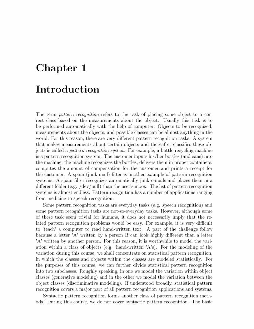
The term pattern recognition refers to the task of placing some object to a cor-rect class based on the measurements about the object. Usually this task is tobe performed automatically with the help of computer. Objects to be recognized,measurements about the objects, and possible classes can be almost anything in theworld. For this reason, there are very different pattern recognition tasks. A systemthat makes measurements about certain objects and thereafter classifies these ob-jects is called a pattern recognition system. For example, a bottle recycling machineis a pattern recognition system. The customer inputs his/her bottles (and cans) intothe machine, the machine recognizes the bottles, delivers them in proper containers,computes the amount of compensation for the customer and prints a receipt forthe customer. A spam (junk-mail) filter is another example of pattern recognitionsystems. A spam filter recognizes automatically junk e-mails and places them in adifferent folder (e.g. /dev/null) than the user’s inbox. The list of pattern recognitionsystems is almost endless. Pattern recognition has a number of applications rangingfrom medicine to speech recognition.
Some pattern recognition tasks are everyday tasks (e.g. speech recognition) andsome pattern recognition tasks are not-so-everyday tasks. However, although someof these task seem trivial for humans, it does not necessarily imply that the re-lated pattern recognition problems would be easy. For example, it is very difficultto ’teach’ a computer to read hand-written text. A part of the challenge followbecause a letter ’A’ written by a person B can look highly different than a letter’A’ written by another person. For this reason, it is worthwhile to model the vari-ation within a class of objects (e.g. hand-written ’A’s). For the modeling of thevariation during this course, we shall concentrate on statistical pattern recognition,in which the classes and objects within the classes are modeled statistically. Forthe purposes of this course, we can further divide statistical pattern recognitioninto two subclasses. Roughly speaking, in one we model the variation within objectclasses (generative modeling) and in the other we model the variation between theobject classes (discriminative modeling). If understood broadly, statistical patternrecognition covers a major part of all pattern recognition applications and systems.
Syntactic pattern recognition forms another class of pattern recognition meth-ods. During this course, we do not cover syntactic pattern recognition. The basic
2 Introduction to Pattern Recognition
idea of syntactic pattern recognition is that the patterns (observations about theobjects to be classified) can always be represented with the help of simpler andsimpler subpatterns leading eventually to atomic patterns which cannot anymorebe decomposed into subpatterns. Pattern recognition is then the study of atomicpatterns and the language between relations of these atomic patterns. The theoryof formal languages forms the basis of syntactic pattern recognition.
Some scholars distinguish yet another type of pattern recognition: The neuralpattern recognition, which utilizes artificial neural networks to solve pattern recog-nition problems. However, artificial neural networks can well be included within theframework of statistical pattern recognition. Artificial neural networks are coveredduring the courses ’Pattern recognition’ and ’Neural computation’.
Chapter 2
Pattern Recognition Systems
2.1 Examples
2.1.1 Optical Character Recognition (OCR)
Optical character recognition (OCR) means recognition of alpha-numeric lettersbased on image-input. The difficulty of the OCR problems depends on whethercharacters to be recognized are hand-written or written out by a machine (printer).The difficulty level of an OCR problem is additionally influenced by the quality ofimage input, if it can be assumed that the characters are within the boxes reservedfor them as in machine readable forms, and how many different characters the systemneeds to recognize.
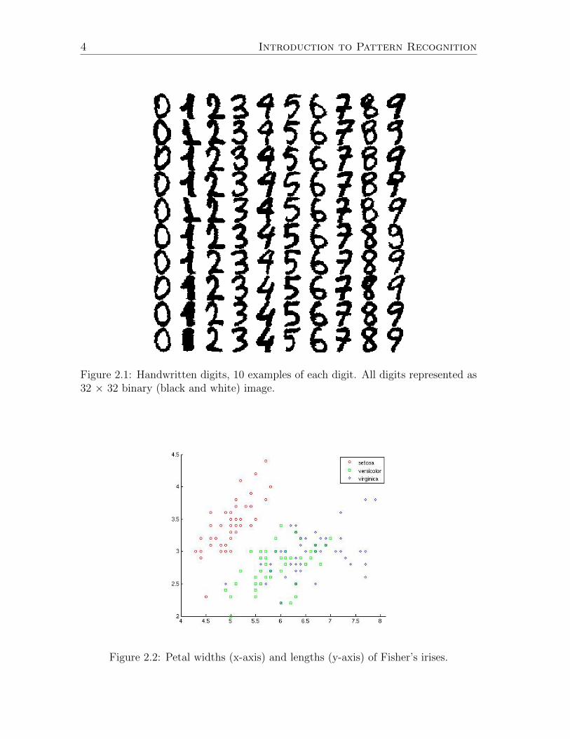
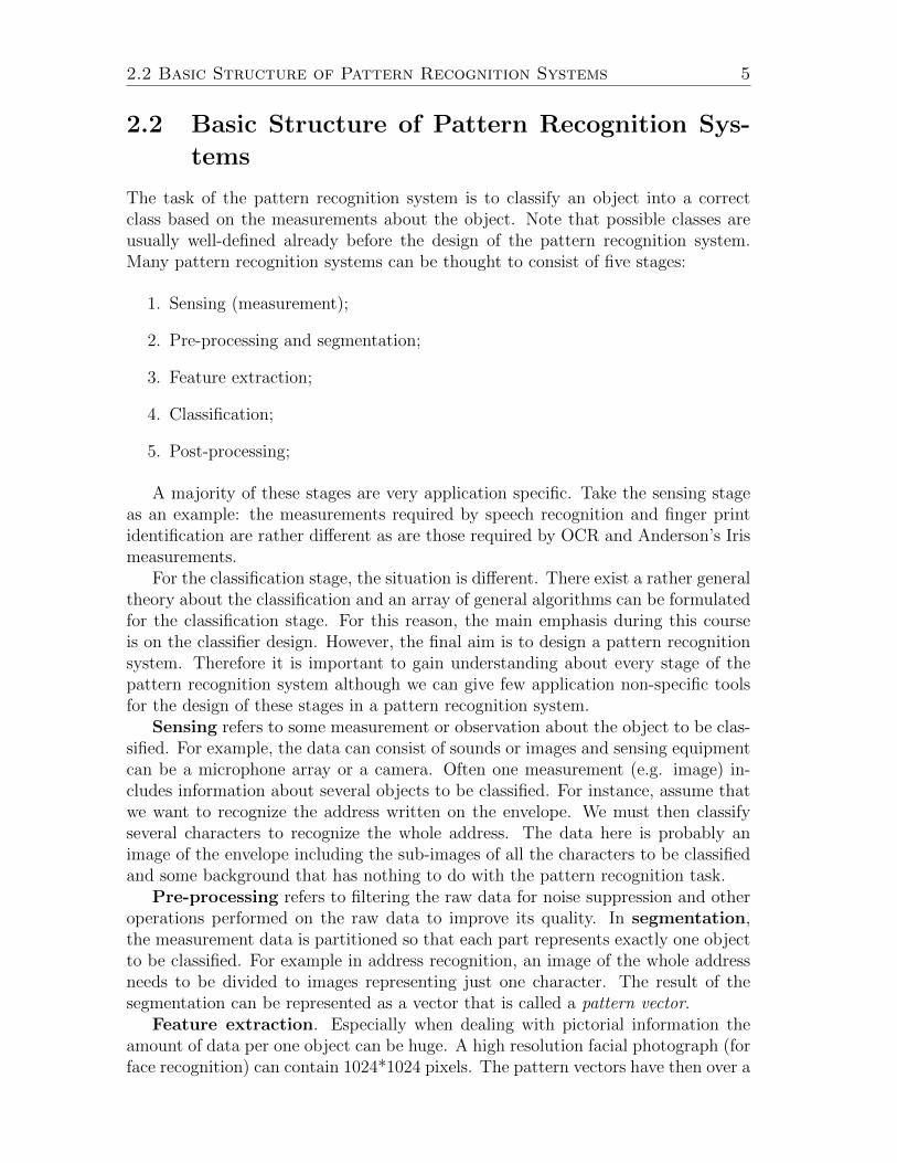
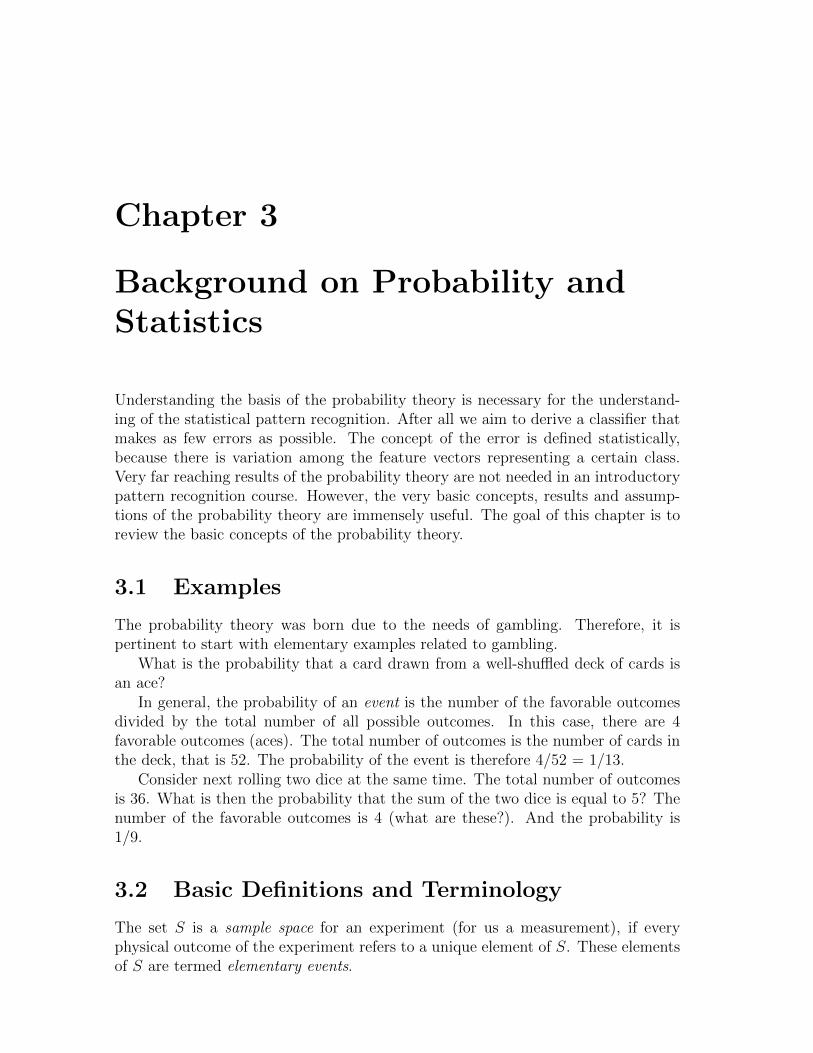
During this course, we will briefly consider the recognition of hand-written nu-merals. The data is freely available from the machine learning database of theUniversity of California, Irvine. The data has been provided by E. Alpaydin and C.Kaynak from the University of Istanbul, see examples in Figure 2.1.
2.1.2 Irises of Fisher/Anderson
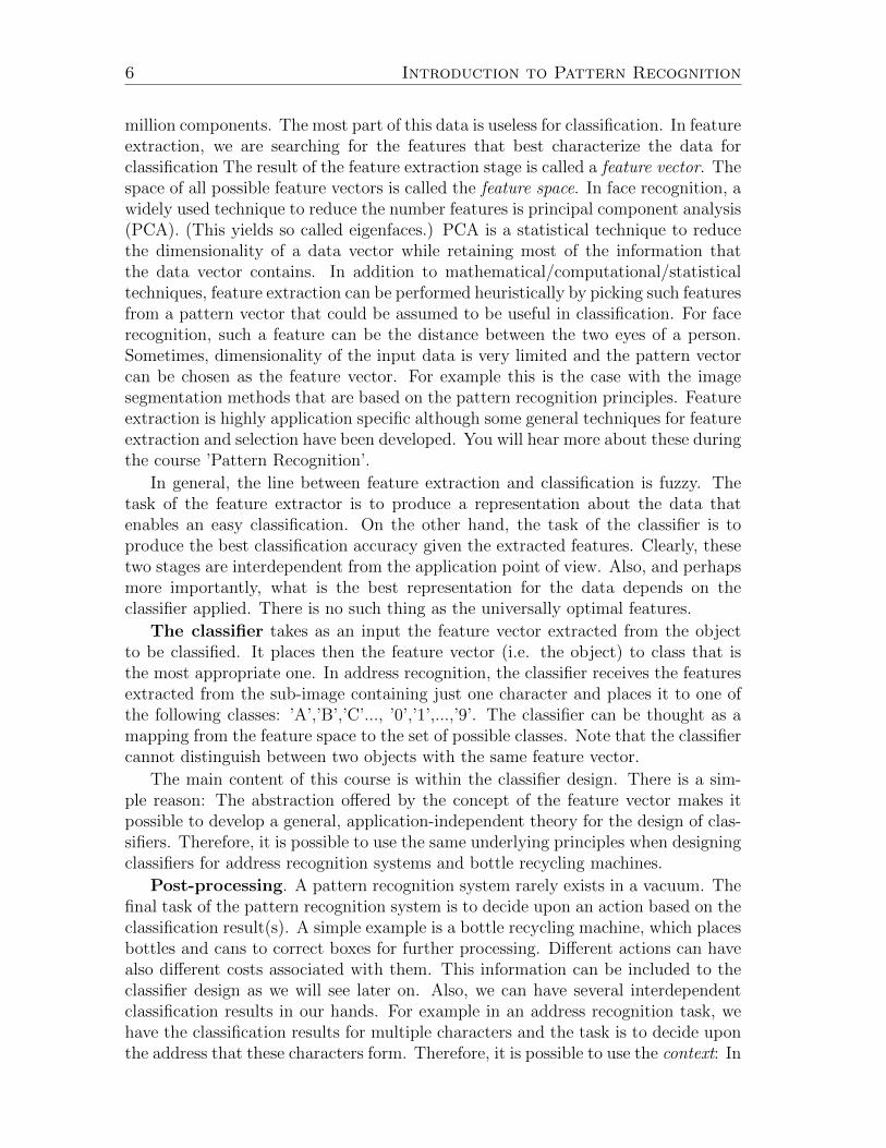
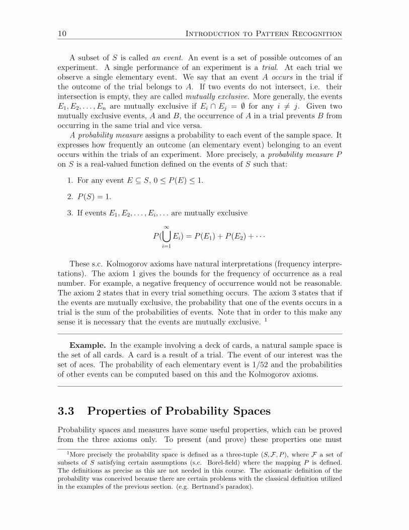
Perhaps the best known material used in the comparisons of pattern classifiers isthe so-called Iris dataset. This dataset was collected by Edgar Anderson in 1935. Itcontains sepal width, sepal length, petal width and petal length measurements from150 irises belonging to three different sub-species. R.A. Fisher made the materialfamous by using it as an example in the 1936 paper ’The use of multiple measure-ments in taxonomic problems’, which can be considered as the first article about thepattern recognition. This is why the material is usually referred as the Fisher’s IrisData instead of the Anderson’s Iris Data. The petal widths and lengths are shownin Figure 2.2.
4 Introduction to Pattern Recognition
Figure 2.1: Handwritten digits, 10 examples of each digit. All digits represented as32 × 32 binary (black and white) image.
Figure 2.2: Petal widths (x-axis) and lengths (y-axis) of Fisher’s irises.
2.2 Basic Structure of Pattern Recognition Systems 5
2.2 Basic Structure of Pattern Recognition Sys-
tems
The task of the pattern recognition system is to classify an object into a correctclass based on the measurements about the object. Note that possible classes areusually well-defined already before the design of the pattern recognition system.Many pattern recognition systems can be thought to consist of five stages:
1. Sensing (measurement);
2. Pre-processing and segmentation;
3. Feature extraction;
4. Classification;
5. Post-processing;
A majority of these stages are very application specific. Take the sensing stageas an example: the measurements required by speech recognition and finger printidentification are rather different as are those required by OCR and Anderson’s Irismeasurements.
For the classification stage, the situation is different. There exist a rather generaltheory about the classification and an array of general algorithms can be formulatedfor the classification stage. For this reason, the main emphasis during this courseis on the classifier design. However, the final aim is to design a pattern recognitionsystem. Therefore it is important to gain understanding about every stage of thepattern recognition system although we can give few application non-specific toolsfor the design of these stages in a pattern recognition system.
Sensing refers to some measurement or observation about the object to be clas-sified. For example, the data can consist of sounds or images and sensing equipmentcan be a microphone array or a camera. Often one measurement (e.g. image) in-cludes information about several objects to be classified. For instance, assume thatwe want to recognize the address written on the envelope. We must then classifyseveral characters to recognize the whole address. The data here is probably animage of the envelope including the sub-images of all the characters to be classifiedand some background that has nothing to do with the pattern recognition task.
Pre-processing refers to filtering the raw data for noise suppression and otheroperations performed on the raw data to improve its quality. In segmentation,the measurement data is partitioned so that each part represents exactly one objectto be classified. For example in address recognition, an image of the whole addressneeds to be divided to images representing just one character. The result of thesegmentation can be represented as a vector that is called a pattern vector.
Feature extraction. Especially when dealing with pictorial information theamount of data per one object can be huge. A high resolution facial photograph (forface recognition) can contain 1024*1024 pixels. The pattern vectors have then over a
6 Introduction to Pattern Recognition
million components. The most part of this data is useless for classification. In featureextraction, we are searching for the features that best characterize the data forclassification The result of the feature extraction stage is called a feature vector. Thespace of all possible feature vectors is called the feature space. In face recognition, awidely used technique to reduce the number features is principal component analysis(PCA). (This yields so called eigenfaces.) PCA is a statistical technique to reducethe dimensionality of a data vector while retaining most of the information thatthe data vector contains. In addition to mathematical/computational/statisticaltechniques, feature extraction can be performed heuristically by picking such featuresfrom a pattern vector that could be assumed to be useful in classification. For facerecognition, such a feature can be the distance between the two eyes of a person.Sometimes, dimensionality of the input data is very limited and the pattern vectorcan be chosen as the feature vector. For example this is the case with the imagesegmentation methods that are based on the pattern recognition principles. Featureextraction is highly application specific although some general techniques for featureextraction and selection have been developed. You will hear more about these duringthe course ’Pattern Recognition’.
In general, the line between feature extraction and classification is fuzzy. Thetask of the feature extractor is to produce a representation about the data thatenables an easy classification. On the other hand, the task of the classifier is toproduce the best classification accuracy given the extracted features. Clearly, thesetwo stages are interdependent from the application point of view. Also, and perhapsmore importantly, what is the best representation for the data depends on theclassifier applied. There is no such thing as the universally optimal features.
The classifier takes as an input the feature vector extracted from the objectto be classified. It places then the feature vector (i.e. the object) to class that isthe most appropriate one. In address recognition, the classifier receives the featuresextracted from the sub-image containing just one character and places it to one ofthe following classes: ’A’,’B’,’C’..., ’0’,’1’,...,’9’. The classifier can be thought as amapping from the feature space to the set of possible classes. Note that the classifiercannot distinguish between two objects with the same feature vector.
The main content of this course is within the classifier design. There is a sim-ple reason: The abstraction offered by the concept of the feature vector makes itpossible to develop a general, application-independent theory for the design of clas-sifiers. Therefore, it is possible to use the same underlying principles when designingclassifiers for address recognition systems and bottle recycling machines.
Post-processing. A pattern recognition system rarely exists in a vacuum. Thefinal task of the pattern recognition system is to decide upon an action based on theclassification result(s). A simple example is a bottle recycling machine, which placesbottles and cans to correct boxes for further processing. Different actions can havealso different costs associated with them. This information can be included to theclassifier design as we will see later on. Also, we can have several interdependentclassification results in our hands. For example in an address recognition task, wehave the classification results for multiple characters and the task is to decide uponthe address that these characters form. Therefore, it is possible to use the context: In
2.3 Design of Pattern Recognition Systems 7
this case, the information about the other classification results to correct a possiblemisclassification. If the result of the classifier is ’Hollywoud Boulevard’ then theaddress is probably ’Hollywood Boulevard’.
2.3 Design of Pattern Recognition Systems
The design of a pattern recognition system is an iterative process. If the systemis not good enough, we go back to the drawing table and try to improve some orall of the five stages of the system (see the previous section 2.2). After that thesystem is tested again and it is improved if it still does not meet the requirementsplaced for it. The process is repeated until the system meets the requirements. Thedesign process is founded on the knowledge about the particular pattern recognitionapplication, the theory of pattern recognition and simply trial and error. Clearly,the smaller the importance of ’trial and error’ the faster is the design cycle. Thismakes it important to minimize the amount of trial and error in the design of thepattern recognition system. The importance of ’trial and error’ can be minimized byhaving good knowledge about the theory of pattern recognition and integrating thatwith knowledge about the application area. When is a pattern recognition systemgood enough? This obviously depends on the requirements of the application, butthere are some general guidelines about how to evaluate the system. We will returnto these later on during this course. How can a system be improved? For example, itcan be possible to add a new feature to feature vectors to improve the classificationaccuracy. However, this is not always possible. For example with the Fisher’s Irisdataset, we are restricted to the four existing features because we cannot influencethe original measurements. Another possibility to improve a pattern recognitionsystem is to improve the classifier. For this too there exists a variety of differentmeans and it might not be a simple task to pick the best one out of these. We willreturn to this dilemma once we have the required background.
When designing a pattern recognition system, there are other factors that needto be considered besides the classification accuracy. For example, the time spent forclassifying an object might be of crucial importance. The cost of the system can bean important factor as well.
2.4 Supervised and Unsupervised Learning and
Classification
The classifier component of a pattern recognition system has to be taught to identifycertain feature vectors to belong to a certain class. The points here are that 1) itis impossible to define the correct classes for all the possible feature vectors1 and 2)
1Think about 16 times 16 binary images where each pixel is a feature, which has either value0 or 1. In this case, we have 2256 ≈ 1077 possible feature vectors. To put it more plainly, we havemore feature vectors in the feature space than there are atoms in this galaxy.
8 Introduction to Pattern Recognition
the purpose of the system is to assign an object which it has not seen previously toa correct class.
It is important to distinguish between two types of machine learning when con-sidering the pattern recognition systems. The (main) learning types are supervisedlearning and unsupervised learning. We also use terms supervised classification andunsupervised classification
In supervised classification, we present examples of the correct classification (afeature vector along with its correct class) to teach a classifier. Based on theseexamples, that are sometimes termed prototypes or training samples, the classifierthen learns how to assign an unseen feature vector to a correct class. The generationof the prototypes (i.e. the classification of feature vectors/objects they represent)has to be done manually in most cases. This can mean lot of work: After all, it wasbecause we wanted to avoid the hand-labeling of objects that we decided to design apattern recognition system in the first place. That is why the number of prototypesis usually very small compared to the number of possible inputs received by thepattern recognition system. Based on these examples we would have to deduct theclass of a never seen object. Therefore, the classifier design must be based on theassumptions made about the classification problem in addition to prototypes used toteach the classifier. These assumptions can often be described best in the languageof probability theory.
In unsupervised classification or clustering, there is no explicit teacher nor train-ing samples. The classification of the feature vectors must be based on similaritybetween them based on which they are divided into natural groupings. Whether anytwo feature vectors are similar depends on the application. Obviously, unsupervisedclassification is a more difficult problem than supervised classification and super-vised classification is the preferable option if it is possible. In some cases, however,it is necessary to resort to unsupervised learning. For example, this is the case ifthe feature vector describing an object can be expected to change with time.
There exists a third type of learning: reinforcement learning. In this learningtype, the teacher does not provide the correct classes for feature vectors but theteacher provides feedback whether the classification was correct or not. In OCR,assume that the correct class for a feature vector is ’R’. The classifier places it into theclass ’B’. In reinforcement learning, the feedback would be that ’the classification isincorrect’. However the feedback does not include any information about the correctclass.
Chapter 3
Background on Probability andStatistics
Understanding the basis of the probability theory is necessary for the understand-ing of the statistical pattern recognition. After all we aim to derive a classifier thatmakes as few errors as possible. The concept of the error is defined statistically,because there is variation among the feature vectors representing a certain class.Very far reaching results of the probability theory are not needed in an introductorypattern recognition course. However, the very basic concepts, results and assump-tions of the probability theory are immensely useful. The goal of this chapter is toreview the basic concepts of the probability theory.
3.1 Examples
The probability theory was born due to the needs of gambling. Therefore, it ispertinent to start with elementary examples related to gambling.
What is the probability that a card drawn from a well-shuffled deck of cards isan ace?
In general, the probability of an event is the number of the favorable outcomesdivided by the total number of all possible outcomes. In this case, there are 4favorable outcomes (aces). The total number of outcomes is the number of cards inthe deck, that is 52. The probability of the event is therefore 4/52 = 1/13.
Consider next rolling two dice at the same time. The total number of outcomesis 36. What is then the probability that the sum of the two dice is equal to 5? Thenumber of the favorable outcomes is 4 (what are these?). And the probability is1/9.
3.2 Basic Definitions and Terminology
The set S is a sample space for an experiment (for us a measurement), if everyphysical outcome of the experiment refers to a unique element of S. These elementsof S are termed elementary events.
10 Introduction to Pattern Recognition
A subset of S is called an event. An event is a set of possible outcomes of anexperiment. A single performance of an experiment is a trial. At each trial weobserve a single elementary event. We say that an event A occurs in the trial ifthe outcome of the trial belongs to A. If two events do not intersect, i.e. theirintersection is empty, they are called mutually exclusive. More generally, the eventsE1, E2, . . . , En are mutually exclusive if Ei ∩ Ej = ∅ for any i 6= j. Given twomutually exclusive events, A and B, the occurrence of A in a trial prevents B fromoccurring in the same trial and vice versa.
A probability measure assigns a probability to each event of the sample space. Itexpresses how frequently an outcome (an elementary event) belonging to an eventoccurs within the trials of an experiment. More precisely, a probability measure Pon S is a real-valued function defined on the events of S such that:
1. For any event E ⊆ S, 0 ≤ P (E) ≤ 1.
2. P (S) = 1.
3. If events E1, E2, . . . , Ei, . . . are mutually exclusive
P (∞⋃i=1
Ei) = P (E1) + P (E2) + · · ·
These s.c. Kolmogorov axioms have natural interpretations (frequency interpre-tations). The axiom 1 gives the bounds for the frequency of occurrence as a realnumber. For example, a negative frequency of occurrence would not be reasonable.The axiom 2 states that in every trial something occurs. The axiom 3 states that ifthe events are mutually exclusive, the probability that one of the events occurs in atrial is the sum of the probabilities of events. Note that in order to this make anysense it is necessary that the events are mutually exclusive. 1
Example. In the example involving a deck of cards, a natural sample space isthe set of all cards. A card is a result of a trial. The event of our interest was theset of aces. The probability of each elementary event is 1/52 and the probabilitiesof other events can be computed based on this and the Kolmogorov axioms.
3.3 Properties of Probability Spaces
Probability spaces and measures have some useful properties, which can be provedfrom the three axioms only. To present (and prove) these properties one must
1More precisely the probability space is defined as a three-tuple (S,F , P ), where F a set ofsubsets of S satisfying certain assumptions (s.c. Borel-field) where the mapping P is defined.The definitions as precise as this are not needed in this course. The axiomatic definition of theprobability was conceived because there are certain problems with the classical definition utilizedin the examples of the previous section. (e.g. Bertnand’s paradox).
3.4 Random Variables and Random Vectors 11
rely mathematical abstraction of the probability spaces offered by their definition.However, as we are more interested in their interpretation, a little dictionary isneeded: In the following E and F are events and Ec denotes the complement of E.
set theory probabilityEc E does not happen
E ∪ F E or F happensE ∩ F E and F both happen
Note that often P (E ∩ F ) is abbreviated as P (E,F ).And some properties:
Theorem 1 Let E and F be events of the sample space S. The probability measureP of S has the following properties:
1. P (Ec) = 1− P (E)
2. P (∅) = 0
3. If E is a sub-event of F :n (E ⊆ F ), then P (F − E) = P (F )− P (E)
4. P (E ∪ F ) = P (E) + P (F )− P (E ∩ F )
If the events F1, . . . , Fn are mutually exclusive and S = F1 ∪ · · · ∪ Fn , then
5. P (E) =∑n
i=1 P (E ∩ Fi).
A collection of events as in the point 5 is called a partition of S. Note that anevent F and its complement F c always form a partition. The proofs of the abovetheorem are simple and they are skipped in these notes. The Venn diagrams can beuseful if the logic behind the theorem seems fuzzy.
3.4 Random Variables and Random Vectors
Random variables characterize the concept of random experiment in probabilitytheory. In pattern recognition , the aim is to assign an object to a correct classbased on the observations about the object. The observations about an objectfrom a certain class can be thought as a trial. The idea behind introducing theconcept of a random variable is that, via it, we can transfer all the considerationsto the space of real numbers R and we do not have to deal separately with separateprobability spaces. In practise, everything we need to know about random variableis its probability distribution (to be defined in next section).
Formally, a random variable (RV) is defined as a real-valued function X definedon a sample space S, i.e. X : S → R. The set of values {X(x) : x ∈ S} taken on byX is called the co-domain or the range of X.
12 Introduction to Pattern Recognition
Example. Recall our first example, where we wanted to compute the probabilityof drawing an ace from a deck of cards. The sample space consisted of the labelsof the cards. A relevant random variable in this case is a map X : labels of cards→ {0, 1}, where X(ace) = 1 and X(notace) = 0 , where notace refers to all thecards that are not aces. When rolling two dice, a suitable RV is e.g. a map fromthe sample space to the sum of two dice.
These are examples of relevant RVs only. There is no unique RV that can berelated to a certain experiment. Instead, there exist several possibilities, some ofwhich are better than others.
Random vectors are generalizations of random variables to multivariate situa-tions. Formally, these are defined as maps X : S → Rd, where d is an integer.For random vectors, the definition of co-domain is a natural extension of the defi-nition of co-domain for random variables. In pattern recognition, the classificationseldom succeeds if we have just one observation/measurement/feature in our dis-posal. Therefore, we are mainly concerned with random vectors. From now on,we do not distinguish between a single variate random variable and a random vec-tor. Both are called random variables unless there is a special need to emphasizemultidimensionality.
We must still connect the concept of the random variable to the concept ofthe probability space. The task of random variables is to transfer the probabilitiesdefined for the subsets of the sample space to the subsets of the Euclidean space:The probability of a subset A of the co-domain of X is equal to the probability ofinverse image of A in the sample space. This makes it possible to model probabilitieswith the probability distributions.
Often, we can just ’forget’ about the sample space and model the probabilitiesvia random variables. The argument of the random variable is often dropped fromthe notation, i.e. P (X ∈ B) is equivalent to P ({s : X(s) ∈ B, s ∈ S,B ⊆ Rd})2.
Note that a value obtained by a random variable reflects a result of a singletrial. This is different than the random variable itself. These two should under nocircumstances be confused although the notation may give possibility to do that.
3.5 Probability Densities and Cumulative Distri-
butions
3.5.1 Cumulative Distribution Function (cdf)
First we need some additional notation: For vectors x = [x1, . . . , xd]T and y =
[y1, . . . , yd]T notation x < y is equivalent to x1 < y1 and x2 < y2 and · · · and
xd < yd. That is, if the components of the vectors are compared pairwise then thecomponents of x are all smaller than components of y.
2For a good and more formal treatment of the issue, see E.R. Dougherty: Probability andStatistics for the Engineering, Computing and Physical Sciences.
3.5 Probability Densities and Cumulative Distributions 13
The cumulative distribution function FX (cdf) of an RV X is defined for all x as
FX(x) = P (X ≤ x) = P ({s : X(s) ≤ x}). (3.1)
The cdf measures the probability mass of all y that are smaller than x.
Example. Let us once again consider the deck of cards and the probability ofdrawing an ace. The RV in this case was the map from the labels of the cards to theset {0, 1} with the value of the RV equal to 1 in the case of a ace and 0 otherwise.Then FX(x) = 0, when x < 0, FX(x) = 48/52, when 0 ≤ x < 1, and FX(x) = 1otherwise.
Theorem 2 The cdf FX has the following properties:
1. FX is increasing, i.e. if x ≤ y, then FX(x) ≤ FX(y).
2. limx→−∞ FX(x) = 0, limx→∞ FX(x) = 1.
3.5.2 Probability Densities: Discrete Case
An RV X is discrete if its co-domain is denumerable. (The elements denumerableset can be written as a list x1,x2,x3, . . .. This list may be finite or infinite).
The probability density function (pdf) pX of a discrete random variable X isdefined as
pX(x) =
{P (X = x) if x belongs to codomain of X0 otherwise
. (3.2)
In other words, a value of the pdf pX(x) is the probability of the event X = x. Ifan RV X has a pdf pX , we say that X is distributed according to pX and we denoteX ∼ pX . The cdf of a discrete RV can we then written as
FX(x) =∑y≤x
pX(y),
where the summation is over y that belong to the co-domain of X.
3.5.3 Probability Densities: Continuous Case
An RV X is continuous if there exists such function pX that
FX(x) =
∫ x
−∞pX(y)dy. (3.3)
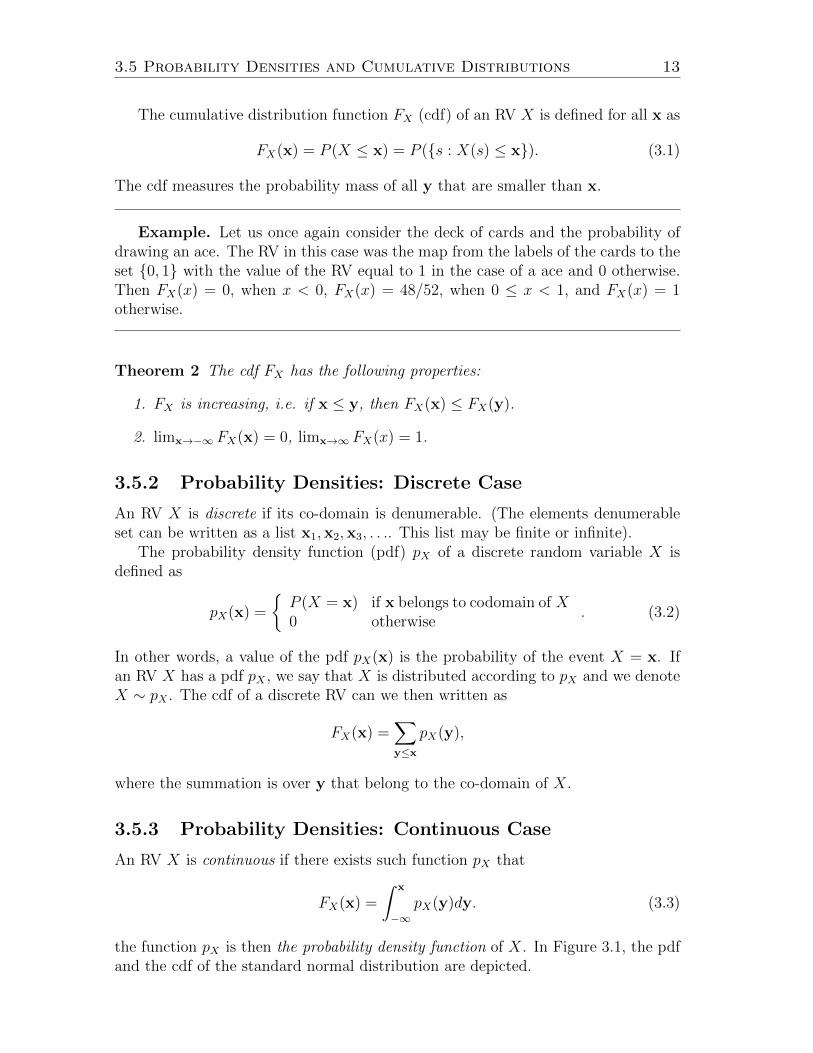
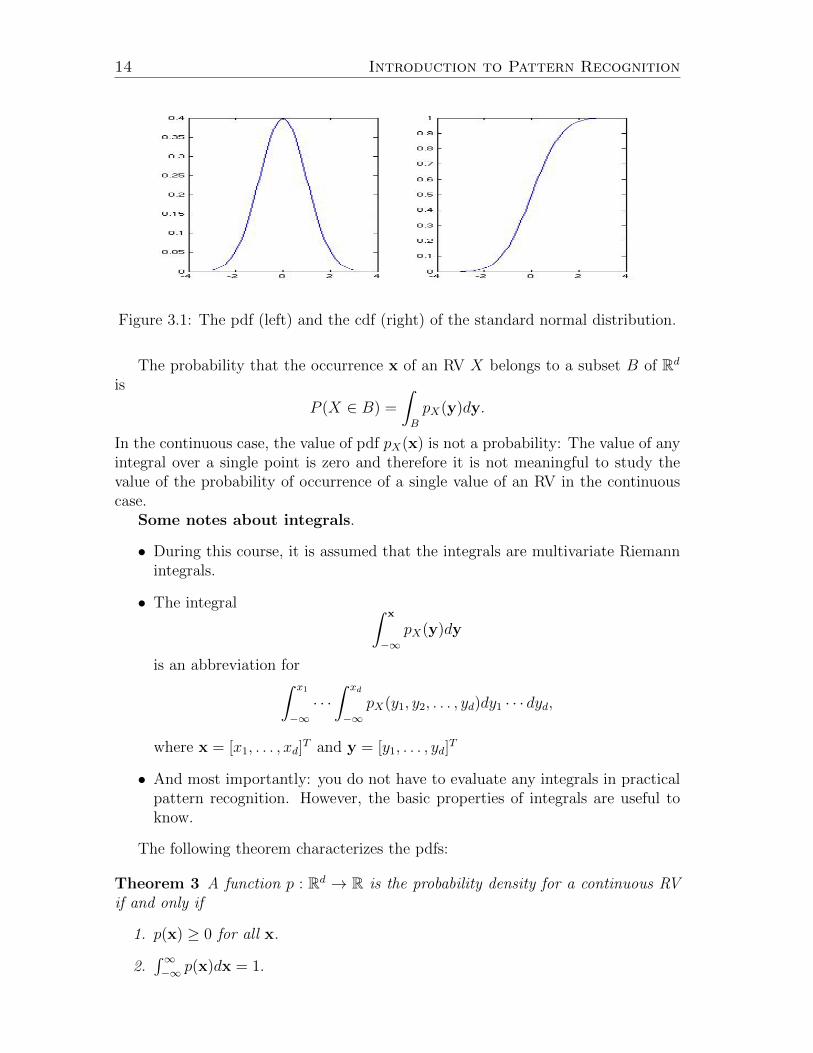
the function pX is then the probability density function of X. In Figure 3.1, the pdfand the cdf of the standard normal distribution are depicted.
14 Introduction to Pattern Recognition
Figure 3.1: The pdf (left) and the cdf (right) of the standard normal distribution.
The probability that the occurrence x of an RV X belongs to a subset B of Rd
is
P (X ∈ B) =
∫B
pX(y)dy.
In the continuous case, the value of pdf pX(x) is not a probability: The value of anyintegral over a single point is zero and therefore it is not meaningful to study thevalue of the probability of occurrence of a single value of an RV in the continuouscase.
Some notes about integrals.
• During this course, it is assumed that the integrals are multivariate Riemannintegrals.
• The integral ∫ x
−∞pX(y)dy
is an abbreviation for∫ x1
−∞· · ·∫ xd
−∞pX(y1, y2, . . . , yd)dy1 · · · dyd,
where x = [x1, . . . , xd]T and y = [y1, . . . , yd]
T
• And most importantly: you do not have to evaluate any integrals in practicalpattern recognition. However, the basic properties of integrals are useful toknow.
The following theorem characterizes the pdfs:
Theorem 3 A function p : Rd → R is the probability density for a continuous RVif and only if
1. p(x) ≥ 0 for all x.
2.∫∞−∞ p(x)dx = 1.
3.6 Conditional Distributions and Independence 15
Let D be the co-domain of a discrete RV X. A function p : D → R is the probabilitydensity for a discrete RV X if and only if
1. p(x) ≥ 0 for all x within the co-domain of X.
2.∑
x p(x) = 1, where the summation runs over the co-domain of X.
The above theorem is a direct consequence of the Kolmogorov axioms. Also, thepdf (if it exists) defines uniquely the random variable. This means that in mostcases all we need is the knowledge about the pdf of an RV.
Finally, the probability density function is the derivative of the cumulative dis-tribution function if the cdf is differentiable. In the multivariate case, the pdf isobtained based on the cdf by differentiating the cdf with respect to all the compo-nents of the vector valued variate.
3.6 Conditional Distributions and Independence
3.6.1 Events
Assume that the events E and F relate to the same experiment. The events E ⊂ Sand F ⊂ S are (statistically) independent if
P (E ∩ F ) = P (E)P (F ). (3.4)
If E and F are not independent, they are dependent. The independence of events Eand F means that an occurrence of E does not affect the likelihood of an occurrenceof F in the same experiment. Assume that P (F ) 6= 0. The conditional probabilityof E relative to F ⊆ S is denoted by P (E|F ) and defined as
P (E|F ) =P (E ∩ F )
P (F ). (3.5)
This refers to the probability of the event E provided that the event F has alreadyoccurred. In other words, we know that the result of a trial was included in theevent F .
If E and F are independent, then
P (E|F ) =P (E ∩ F )
P (F )=P (E)P (F )
P (F )= P (E).
Accordingly, if P (E|F ) = P (E), then
P (E ∩ F ) = P (E)P (F ), (3.6)
and events E and F are independent. The point is that an alternative definition ofindependence can be given via conditional probabilities. Note also that the conceptof independence is different from the concept of mutual exclusivity. Indeed, if the
16 Introduction to Pattern Recognition
events E and F are mutually exclusive, then P (E|F ) = P (F |E) = 0, and E and Fare dependent.
Definition (3.4) does not generalize in a straight-forward manner. The indepen-dence of the events E1, . . . , En must be defined inductively. Let K = {i1, i2, . . . , ik}be an arbitrary subset of the index set {1, . . . , n}. The events E1, . . . , En are inde-pendent if it holds for every K ⊂ {1, . . . , n} that
P (Ei1 ∩ · · · ∩ Eik) = P (Ei1) · · ·P (Eik). (3.7)
Assume that we have more than two events, say E,F and G. They are pairwiseindependent if E and F are independent and F and G are independent and E and Gare independent. However, it does not follow from the pairwise independence thatE,F and G would be independent. The definition of the statistical independence ismore easily defined by random variables and their pdfs as we shall see in the nextsubsection.
3.6.2 Random Variables
Let us now study the random variables X1, X2, . . . , Xn related to the same experi-ment. We define a random variable
X = [XT1 , X
T2 , . . . , X
Tn ]T .
(X is a vector of vectors). The pdf
pX(x) = p(X1,...,Xn)(x1,x2, . . . ,xn)
is the joint probability density function of the RVs X1, X2, . . . , Xn. The value
p(X1,...,Xn)(x1,x2, . . . ,xn)
refers to the probability density of X1 receiving the value x1, X2 receiving the valuex2 and so forth in a trial. The pdfs pXi
(xi) are called the marginal densities of X.These are obtained from the joint density by integration. The joint and marginaldistributions have all the properties of pdfs.
The random variables X1, X2, . . . , Xn are independent if and only if
pX(x) = p(X1,...,Xn)(x1,x2, . . . ,xn) = pX1(x1) · · · pXn(xn). (3.8)
Let Ei i = 1, . . . , n and Fj, j = 1, . . . ,m be events related to X1 and X2, respec-tively. Assume that X1 and X2 are independent, Then also all the events related tothe RVs X1 and X2 are independent, i.e.
P (Ei ∩ Fj) = P (Ei)P (Fj),
for all i and j. That is to say that the results of the (sub)experiments modeled byindependent random variables are not dependent on each other. The independence
3.7 Bayes Rule 17
of the two (or more) RVs can be defined with the help of the events related to theRVs. This definition is equivalent to the definition by the pdfs.
It is natural to attach the concept of conditional probability to random variables.We have RVs X and Y . A new RV modeling the probability of X assuming thatwe already know that Y = y is denoted by X|y. It is called the conditional randomvariable of X given y. The RV X|y has a density function defined by
pX|Y (x|y) =pX,Y (x,y)
pY (y). (3.9)
RVs X and Y are independent if and only if
pX|Y (x,y) = pX(x)
for all x,y.
3.7 Bayes Rule
This section is devoted to a very important statistical result to pattern recognition.This Bayes Rule was named after Thomas Bayes (1702 - 1761). This rule has versionsconcerning events and RVs, which both are represented. The derivations here arecarried out only for the case concerning events.
We shall now derive the Bayes rule. Multiplying by P (F ) the both sides of thedefinition of the conditional probability for events E and F yields
P (E ∩ F ) = P (F )P (E|F ).
For this we have assumed that P (F ) > 0. If also P (E) > 0, then
P (E ∩ F ) = P (E)P (F |E).
Combining the two equations yields
P (F )P (E|F ) = P (E ∩ F ) = P (E)P (F |E).
And furthermore
P (F |E) =P (F )P (E|F )
P (E).
This is the Bayes rule. A different formulation of the rule is obtained via the point5 in the Theorem 1. If the events F1, . . . , Fn are mutually exclusive and the samplespace S = F1 ∪ · · · ∪ Fn , then for all k it holds that
P (Fk|E) =P (Fk)P (E|Fk)
P (E)=
P (Fk)P (E|Fk)∑ni=1 P (Fi)P (E|Fi)
.
We will state these results and the corresponding ones for the RVs in a theorem:
18 Introduction to Pattern Recognition
Theorem 4 Assume that E,F, F1, . . . , Fn are events of S. Moreover F1, . . . , Fnform a partition of S, and P (E) > 0, P (F ) > 0. Then
1. P (F |E) = P (F )P (E|F )P (E)
;
2. P (Fk|E) = P (Fk)P (E|Fk)∑ni=1 P (Fi)P (E|Fi)
.
Assume that X and Y are RVs related to the same experiment. Then
3. pX|Y (x|y) =pX(x)pY |X(y|x)
pY (y);
4. pX|Y (x|y) =pX(x)pY |X(y|x)∫pX(x)pY |X(y|x)dx .
Note that the points 3 and 4 hold even if one of the RVs was discrete and theother was continuous. Obviously, it can be necessary to replace the integral by asum.
3.8 Expected Value and Variance
We take a moment to define the concepts of expected value and variance, becausewe will later on refer to these concepts. The expected value of the continuous RVX is defined as
E[X] =
∫ ∞−∞
xpX(x)dx.
The expected value of the discrete RV X is defined as
E[X] =∑x∈DX
xpX(x),
where DX is co-domain of X. Note that if X is a d-component RV then also E[X]is a d-component vector.
The variance of the continuous RV X is defined as
V ar[X] =
∫ ∞−∞
(x− E[X])(x− E[X])TpX(x)dx.
The variance of the discrete RV X is defined as
V ar[X] =∑x∈DX
(x− E[X])(x− E[X])TpX(x),
where DX is co-domain of X. The variance of X is a d× d matrix. In particular, ifX ∼ N(µ,Σ), then E[X] = µ and V ar[X] = Σ.
3.9 Multivariate Normal Distribution 19
3.9 Multivariate Normal Distribution
The multivariate normal distribution is widely used in pattern recognition and statis-tics. Therefore, we have a closer look into this distribution. First, we need the defi-nition for positive definite matrices: Symmetric d × d matrix A is positive-definiteif for all non-zero x ∈ Rd it holds that
xTAx > 0.
Note that, for the above inequality to make sense, the value of the quadratic formxTAx =
∑di=1
∑dj=1 aijxixj must be a scalar. This implies that x must be a column-
vector (i.e. a tall vector). A positive definite matrix is always non-singular and thusit has the inverse matrix. Additionally, the determinant of a positive definite matrixis always positive.
Example. The matrix
B =
2 0.2 0.10.2 3 0.50.1 0.5 4
is positive-definite. We illustrate the calculation of the value of a quadratic form by
selecting x =[−2 1 3
]T. Then
xTBx = 2 · (−2) · (−2) + 0.2 · 1 · (−2) + 0.1 · 3 · (−2)
+ 0.2 · (−2) · 1 + 3 · 1 · 1 + 0.5 · 3 · 1+ 0.1 · (−2) · 3 + 0.5 · 1 · 3 + 4 · 3 · 3= 48.
A d-component RV X ∼ N(µ,Σ) distributed according the normal distributionhas a pdf
pX(x) =1
(2π)d/2√
det(Σ)exp[−1
2(x− µ)TΣ−1(x− µ)], (3.10)
where the parameter µ is a d component vector (the mean of X) and Σ is a d × dpositive definite matrix (the covariance of X). Note that because Σ is positivedefinite, also Σ−1 is positive definite (the proof of this is left as an exercise). Fromthis it follows that 1
2(x− µ)TΣ−1(x− µ) is always non-negative and zero only when
x = µ. This is important since it ensures that the pdf is bounded from above. Themode of the pdf is located at µ. The determinant det(Σ) > 0 and therefore pX(x) > 0for all x. Also,
∫pX(x)dx = 1 (the proof of this is skipped, for the 1-dimensional
case, see e.g. http://mathworld.wolfram.com/GaussianIntegral.html). Hence,the density in (3.10) is indeed a proper probability density.
20 Introduction to Pattern Recognition
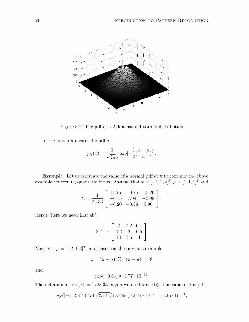
Figure 3.2: The pdf of a 2-dimensional normal distribution
In the univariate case, the pdf is
pX(x) =1√2πσ
exp[−1
2(x− µσ
)2].
Example. Let us calculate the value of a normal pdf at x to continue the aboveexample concerning quadratic forms. Assume that x = [−1, 2, 4]T , µ = [1, 1, 1]T and
Σ =1
23.33
11.75 −0.75 −0.20−0.75 7.99 −0.98−0.20 −0.98 5.96
.Hence (here we need Matlab),
Σ−1 =
2 0.2 0.10.2 3 0.50.1 0.5 4
Now, x− µ = [−2, 1, 3]T , and based on the previous example
s = (x− µ)TΣ−1(x− µ) = 48
andexp(−0.5s) ≈ 3.77 · 10−11.
The determinant det(Σ) = 1/23.33 (again we used Matlab). The value of the pdf
pX([−1, 2, 4]T ) ≈ (√
23.33/15.7496) · 3.77 · 10−11 = 1.16 · 10−11,
3.9 Multivariate Normal Distribution 21
which is extremely small value. Two notes are in order: 1) Remember that the valueof a pdf at a single point is not a probability of any event. However, computingvalues of pdfs like this one is commmon in pattern recognition as we will see in thenext chapter. 2) All calculations like these are performed numerically and using acomputer, the manual computations presented here are just for illustration.
The normal distribution has some interesting properties that make it specialamong the distributions of continuous random variables. Some of them are worthof knowing for this course. In what follows, we denote the components of µ by µiand the components of Σ by σij. If X ∼ N(µ,Σ) then
• sub-variables X1, . . . , Xd of X are normally distributed: Xi ∼ N(µi, σii);
• sub-variables Xi and Xj of X are independent if and only if σij = 0.
• Let A and B be non-singular d× d matrices. Then AX ∼ N(Aµ,AΣAT ) andRVs AX and BX are independent if and only if AΣBT is the zero-matrix.
• The sum of two normally distributed RVs is normally distributed.

22 Introduction to Pattern Recognition
Chapter 4
Bayesian Decision Theory andOptimal Classifiers
The Bayesian decision theory offers a solid foundation for classifier design. It tellsus how to design the optimal classifier when the statistical properties of the classi-fication problem are known. The theory is a formalization of some common-senseprinciples, but it offers a good basis for classifier design.
About notation. In what follows we are a bit more sloppy with the notationthan previously. For example, pdfs are not anymore indexed with the symbol of therandom variable they correspond to.
4.1 Classification Problem
Feature vectors x that we aim to classify belong to the feature space. The featurespace is usually d-dimensional Euclidean space Rd. However, the feature space canbe for instance {0, 1}d, the space formed by the d-bit binary numbers. We denotethe feature space with the symbol F.
The task is to assign an arbitrary feature vector x ∈ F to one of the c classes1
The c classes are denoted by ω1, . . . , ωc and these are assumed to be known. Notethat we are studying a pair of random variables (X,ω), where X models the valueof the feature vector and ω models its class.
We know the
1. prior probabilities P (ω1), . . . , P (ωc) of the classes and
2. the class conditional probability density functions p(x|ω1), . . . , p(x|ωc).
1To be precise, the task is to assign the object that is represented by the feature vector toa class. Hence, what we have just said is not formally true. However, it is impossible for theclassifier to distinguish between two objects with the same feature vector and it is reasonable tospeak about the feature vectors instead of the object they represent. This is also typical in theliterature. In some cases, this simplification of the terminology might lead to misconceptions andin these situations we will use more formal terminology.
24 Introduction to Pattern Recognition
The prior probability P (ωi) defines what percentage of all feature vectors belongto the class ωi. The class conditional pdf p(x|ωi), as it is clear from the notation,defines the pdf of the feature vectors belonging to ωi. This is same as the densityof X given that the class is ωi. To be precise: The marginal distribution of ω isknown and the distributions of X given ωi are known for all i. The general laws ofprobability obviously hold. For example,
c∑i=1
P (ωi) = 1.
We denote a classifier by the symbol α. Because the classification problem isto assign an arbitrary feature vector x ∈ F to one of c classes, the classifier is afunction from the feature space onto the set of classes, i.e. α : F → {ω1, . . . , ωc}.The classification result for the feature vector x is α(x). We often call a function αa decision rule.
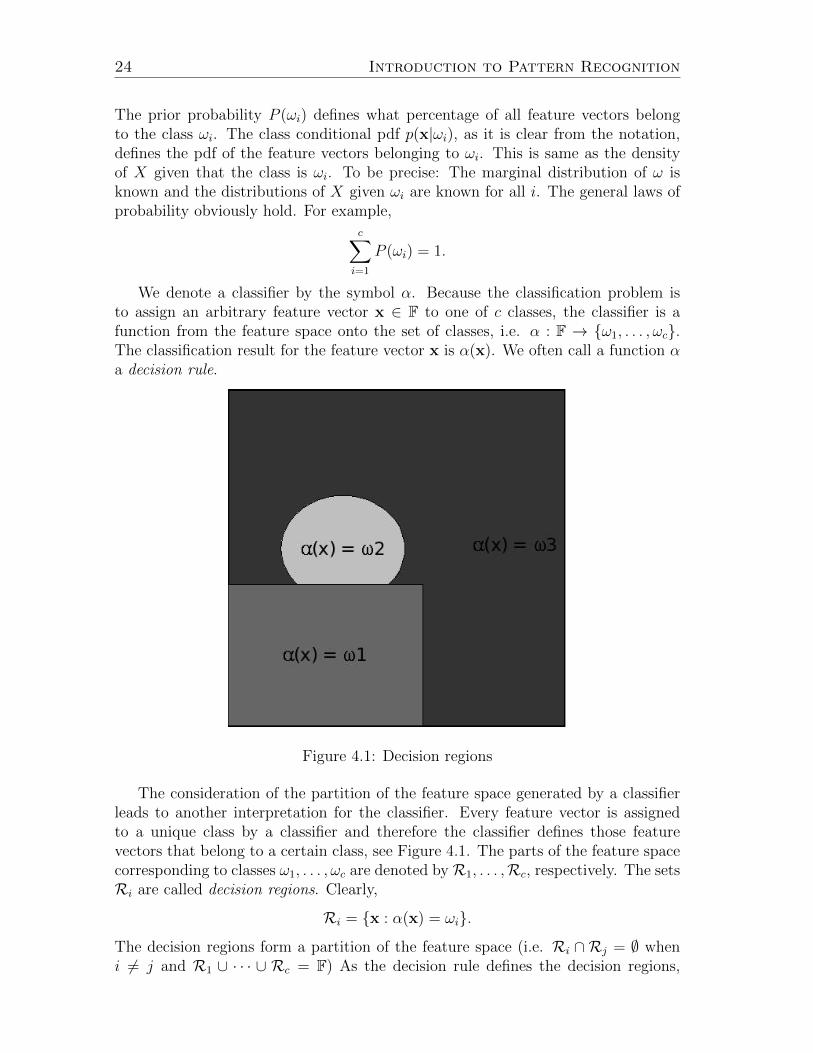
Figure 4.1: Decision regions
The consideration of the partition of the feature space generated by a classifierleads to another interpretation for the classifier. Every feature vector is assignedto a unique class by a classifier and therefore the classifier defines those featurevectors that belong to a certain class, see Figure 4.1. The parts of the feature spacecorresponding to classes ω1, . . . , ωc are denoted byR1, . . . ,Rc, respectively. The setsRi are called decision regions. Clearly,
Ri = {x : α(x) = ωi}.
The decision regions form a partition of the feature space (i.e. Ri ∩ Rj = ∅ wheni 6= j and R1 ∪ · · · ∪ Rc = F) As the decision rule defines the decision regions,
4.2 Classification Error 25
the decision regions define the decision rule: The classifier can be represented byits decision regions. However, especially for large d, the representation by decisionregions is not convenient. However, the representation by decision regions oftenoffers additional intuition on how the classifier works.
4.2 Classification Error
The classification problem is by nature statistical. Objects having same featurevectors can belong to different classes. Therefore, we cannot assume that it wouldbe possible to derive a classifier that works perfectly. (The perfect classifier wouldassign every object to the correct class). This is why we must study the classificationerror: For a specified classification problem our task to derive classifier that makesas few errors (misclassifications) as possible. We denote the classification error bythe decision rule α by E(α). Because the classifier α assigns an object to a classonly based on the feature vector of that object, we study the probability E(α(x)|x)that objects with the feature vector x are misclassified.
Let us take a closer look into the classification error and show that it can becomputed if the preliminary assumptions of the previous section hold. From theitem 1 in Theorem 1, it follows that
E(α(x)|x) = 1− P (α(x)|x), (4.1)
where P (α(x)|x) is the probability that the class α(x) is correct for the object. Theclassification error for the classifier α can be written as
E(α) =
∫FE(α(x)|x)p(x)dx =
∫F[1− P (α(x)|x)]p(x)dx. (4.2)
We need to still know P (α(x)|x). From the Bayes rule we get
P (α(x)|x) =p(x|α(x))P (α(x))
p(x). (4.3)
And hence the classification error is
E(α) = 1−∫Fp(x|α(x))P (α(x))dx, (4.4)
where p(x|α(x)), P (α(x)) are known for every x as it was defined in the previoussection. Note that
p(x|α(x))P (α(x)) = p(x, α(x)).
That is, the classification error of α is equal to the probability of the complementof the event {(x, α(x)) : x ∈ F}.
With the knowledge of decision regions, we can rewrite the classification error as
E(α) =c∑i=1
∫Ri
[1− p(x|ωi)P (ωi)]dx = 1−c∑i=1
∫Ri
p(x|ωi)P (ωi)dx, (4.5)
where Ri, i = 1, . . . , c are decision regions for the decision rule α.
26 Introduction to Pattern Recognition
4.3 Bayes Minimum Error Classifier
In this section, we study Bayes minimum error classifier which, provided that theassumptions of section 4.1 hold, minimizes the classification error. (The assumptionswere that class conditional pdfs and prior probabilities are known.) This means thatBayes minimum error classifier, later on just Bayes classifier, is optimal for a givenclassification problem.
The Bayes classifier is defined as
αBayes(x) = arg maxωi,i=1,...,c
P (ωi|x). (4.6)
Notation arg maxx f(x) means the value of the argument x that yields the maximumvalue for the function f . For example, if f(x) = −(x− 1)2, then arg maxx f(x) = 1(and max f(x) = 0). In other words,
the Bayes classifier selects the most probable class when the observedfeature vector is x.
The posterior probability P (ωi|x) is evaluated based on the Bayes rule, i.e. P (ωi|x) =p(x|ωi)P (ωi)
p(x). Note additionally that p(x) is equal for all classes and p(x) ≥ 0 for all
x and we can multiply the right hand side of (4.6) without changing the classifier.The Bayes classifier can be now rewritten as
αBayes(x) = arg maxωi,i=1,...,c
p(x|ωi)P (ωi). (4.7)
If two or more classes have the same posterior probability given x, we can freelychoose between them. In practice, the Bayes classification of x is performed bycomputing p(x|ωi)P (ωi) for each class ωi, i = 1, . . . , c and assigning x to the classwith the maximum p(x|ωi)P (ωi).
By its definition the Bayes classifier minimizes the conditional error E(α(x)|x) =1− P (α(x)|x) for all x. Because of this and basic properties of integrals, the Bayesclassifier minimizes also the classification error:
Theorem 5 Let α : F → {ω1, . . . , ωc} be an arbitrary decision rule and αBayes :F→ {ω1, . . . , ωc} the Bayes classifier. Then
E(αBayes) ≤ E(α).
The classification error E(αBayes) of the Bayes classifier is called the Bayes error.It is the smallest possible classification error for a fixed classification problem. TheBayes error is
E(αBayes) = 1−∫F
maxi
[p(x|ωi)P (ωi)]dx (4.8)
Finally, note that the definition of the Bayes classifier does not require the as-sumption that the class conditional pdfs are Gaussian distributed. The class condi-tional pdfs can be any proper pdfs.
4.4 Bayes Minimum Risk Classifier 27
4.4 Bayes Minimum Risk Classifier
The Bayes minimum error classifier is a special case of the more general Bayesminimum risk classifier. In addition to the assumptions and terminology introducedpreviously, we are given a actions α1, . . . , αa. These correspond to the actions thatfollow the classification. For example, a bottle recycling machine, after classifyingthe bottles and cans, places them in the correct containers and returns a receipt tothe customer. The actions are tied to the classes via a loss function λ. The valueλ(αi|ωj) quantifies the loss incurred by taking an action αi when the true class is ωj.The decision rules are now functions from the feature space onto the set of actions.We need still one more definition. The conditional risk of taking the action αi whenthe observed feature vector is x is defined as
R(αi|x) =c∑j=1
λ(αi|ωj)P (ωj|x). (4.9)
The definition of the Bayes minimum risk classifier is then:
The Bayes minimum risk classifier chooses the action with the minimumconditional risk.
The Bayes minimum risk classifier is the optimal in this more general setting: itis the decision rule that minimizes the total risk given by
Rtotal(α) =
∫R(α(x)|x)p(x)dx. (4.10)
The Bayes classifier of the previous section is obtained when the action αi is theclassification to the class ωi and the loss function is zero-one loss:
λ(αi|ωj) =
{0 if i = j1 if i 6= j
.
The number of actions a can be different from the number of classes c. Thisis useful e.g. when it is preferable that the pattern recognition system is able toseparate those feature vectors that cannot be reliably classified.
Example. An example about spam filtering illustrates the differences betweenthe minimum error and the minimum risk classification. An incoming e-mail iseither a normal (potentially important) e-mail (ω1) or a junk mail (ω2). We havetwo actions: α1 (keep the mail) and α2 (put the mail to /dev/null). Because losinga normal e-mail is on average three times more painful than getting a junk mail intothe inbox, we select a loss function
λ(α1|ω1) = 0 λ(α1|ω2) = 1λ(α1|ω2) = 3 λ(α2|ω2) = 0
.
28 Introduction to Pattern Recognition
(You may disagree about the loss function.) In addition, we know that P (ω1) =0.4, P (ω2) = 0.6. Now, an e-mail has been received and its feature vector is x. Basedon the feature vector, we have computed p(x|ω1) = 0.35, p(x|ω2) = 0.65.
The posterior probabilities are:
P (ω1|x) =0.35 · 0.4
0.35 · 0.4 + 0.65 · 0.6= 0.264;
P (ω2|x) = 0.736.
For the minimum risk classifier, we must still compute the conditional losses:
R(α1|x) = 0 · 0.264 + 0.736 = 0.736,
R(α2|x) = 0 · 0.736 + 3 · 0.264 = 0.792.
The Bayes (minimum error) classifier classifies the e-mail as spam but the min-imum risk classifier still keeps it in the inbox because of the smaller loss of thataction.
After this example, we will concentrate only on the minimum error classification.However, many of the practical classifiers that will be introduced generalize easilyto the minimum risk case.
4.5 Discriminant Functions and Decision Surfaces
We have already noticed that the same classifier can be represented in several dif-ferent ways, e.g. compare (4.6) and (4.7) which define the same Bayes classifier.As always, we would like this representation be as simple as possible. In general, aclassifier can be defined with the help of a set of discriminant functions. Each classωi has its own discriminant function gi that takes a feature vector x as an input.The classifier assigns the feature vector x to the class with the highest gi(x). Inother words, the class is ωi if
gi(x) > gj(x)
for all i 6= j.For the Bayes classifier, we can select discriminant functions as:
gi(x) = P (ωi|x), i = 1, . . . , c
or as
gi(x) = p(x|ωi)P (ωi), i = 1, . . . , c.
The word ’select’ appears above for a reason: Discriminant functions for a certainclassifier are not uniquely defined. Many different sets of discriminant functions maydefine exactly the same classifier. However, a set of discriminant functions define aunique classifier (but not uniquely). The next result is useful:
4.5 Discriminant Functions and Decision Surfaces 29
Theorem 6 Let f : R → R be increasing, i.e. f(x) < f(y) always when x < y.Then the following sets of discriminant functions
gi(x), i = 1, . . . , c
andf(gi(x)), i = 1, . . . , c
define the same classifier.
This means that discriminant functions can be multiplied by positive constants,constants can be added to them or they can be replaced by their logarithms withoutaltering the underlying classifier.
Later on, we will study discriminant functions of the type
gi(x) = wTi x + wi0.
These are called linear discriminant functions. Above wi is a vector of the equaldimensionality with feature vector and wi0 is a scalar. A linear classifier is a clas-sifier that can be represented by using only linear discriminant functions. Lineardiscriminant functions can be conceived as the most simple type of discriminantfunctions. This explains the interest in linear classifiers.
When the classification problem has just two classes, we can represent the clas-sifier using a single discriminant function
g(x) = g1(x)− g2(x). (4.11)
If g(x) > 0, then x is assigned to ω1 and otherwise x is assigned to ω2.The classifier divides the feature space into parts corresponding classes. The
decision regions can be defined with the help of discriminant functions as follows:
Ri = {x| gi(x) > gj(x), i 6= j}.
The boundaries between decision regions
Rij = {x : gi(x) = gj(x), gk(x) < gi(x), k 6= i, j}
are called decision surfaces. It is easier to grasp the geometry of the classifier (i.e.the partition of the feature space by the classifier) based on decision surfaces thanbased on decision regions directly. For example, it easy to see that the decisionsurfaces of linear classifiers are segments of lines between the decision regions.
Example. Consider a two-class classification problem with P (ω1) = 0.6, P (ω2) =0.4, p(x|ω1) = 1√
2πexp[−0.5x2] and p(x|ω2) = 1√
2πexp[−0.5(x− 1)2]. Find the deci-
sion regions and boundaries for the minimum error rate Bayes classifier.The decision region R1 is the set of points x for which P (ω1|x) > P (ω2|x). The
decision region R2 is the set of points x for which P (ω2|x) > P (ω1|x). The decisionboundary is the set of points x for which P (ω2|x) = P (ω1|x).
30 Introduction to Pattern Recognition
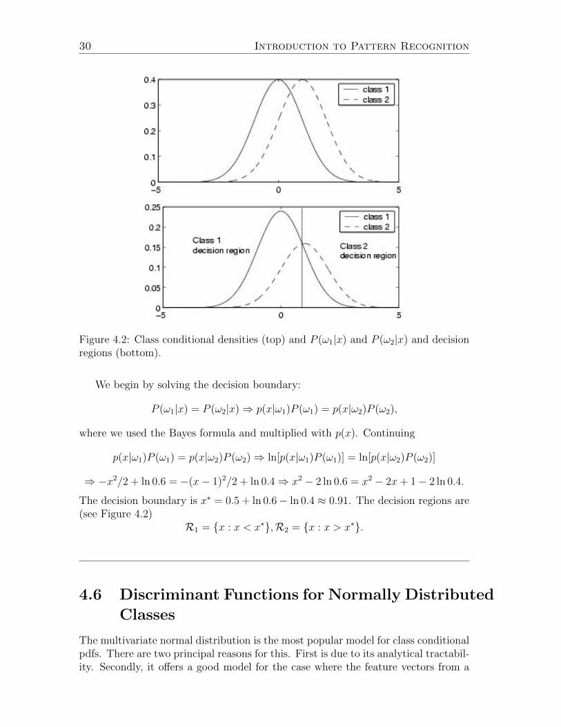
Figure 4.2: Class conditional densities (top) and P (ω1|x) and P (ω2|x) and decisionregions (bottom).
We begin by solving the decision boundary:
P (ω1|x) = P (ω2|x)⇒ p(x|ω1)P (ω1) = p(x|ω2)P (ω2),
where we used the Bayes formula and multiplied with p(x). Continuing
p(x|ω1)P (ω1) = p(x|ω2)P (ω2)⇒ ln[p(x|ω1)P (ω1)] = ln[p(x|ω2)P (ω2)]
⇒ −x2/2 + ln 0.6 = −(x− 1)2/2 + ln 0.4⇒ x2 − 2 ln 0.6 = x2 − 2x+ 1− 2 ln 0.4.
The decision boundary is x∗ = 0.5 + ln 0.6− ln 0.4 ≈ 0.91. The decision regions are(see Figure 4.2)
R1 = {x : x < x∗},R2 = {x : x > x∗}.
4.6 Discriminant Functions for Normally Distributed
Classes
The multivariate normal distribution is the most popular model for class conditionalpdfs. There are two principal reasons for this. First is due to its analytical tractabil-ity. Secondly, it offers a good model for the case where the feature vectors from a
4.6 Discriminant Functions for Normally Distributed Classes 31
certain class can be thought as noisy versions of some average vector typical to theclass. In this section, we study the discriminant functions, decision regions and de-cision surfaces of the Bayes classifier when the class conditional pdfs are modeled bynormal densities. The purpose of this section is to illustrate the concepts introducedand hence special attention should be given to the derivations of the results.
The pdf of the multivariate normal distribution is
pnormal(x|µ,Σ) =1
(2π)d/2√
det(Σ)exp[−1
2(x− µ)TΣ−1(x− µ)], (4.12)
where µ ∈ Rd and positive definite d× d matrix Σ are the parameters of the distri-bution.
We assume that the class conditional pdfs are normally distributed and priorprobabilities can be arbitrary. We denote the parameters for the class conditionalpdf for ωi by µi,Σi i.e. p(x|ωi) = pnormal(x|µi,Σi).
We begin with the Bayes classifier defined in Eq. (4.7). This gives the discrimi-nant functions
gi(x) = pnormal(x|µi,Σi)P (ωi). (4.13)
By replacing these with their logarithms (c.f. Theorem 6) and substituting thenormal densities, we obtain2
gi(x) = −1
2(x− µi)TΣ−1i (x− µi)−
d
2ln 2π − 1
2ln det(Σi) + lnP (ωi). (4.14)
We distinguish three distinct cases:
1. Σi = σ2I, where σ2 is a scalar and I is the identity matrix;
2. Σi = Σ, i.e. all classes have equal covariance matrices;
3. Σi is arbitrary.
Case 1
Dropping the constants from the right hand side of Eq. (4.14) yields
gi(x) = −1
2(x− µi)T (σ2I)−1(x− µi) + lnP (ωi) = −||x− µi||
2
2σ2+ lnP (ωi), (4.15)
The symbol || · || denotes the Euclidean norm, i.e.
||x− µi||2 = (x− µi)T (x− µi).
Expanding the norm yields
gi(x) = − 1
2σ2(xTx− 2µTi x + µTi µi) + lnP (ωi). (4.16)
2Note that the discriminant functions gi(x) in (4.13) and (4.14) are not same functions. gi(x)is just a general symbol for the discriminant functions of the same classifier. However, a moreprudent notation would be a lot messier.
32 Introduction to Pattern Recognition
The term xTx is equal for all classes so it can be dropped. This gives
gi(x) =1
σ2(µTi x− 1
2µTi µi) + lnP (ωi), (4.17)
which is a linear discriminant function with
wi =µiσ2,
and
wi0 =−µTi µ2σ2
+ P (ωi).
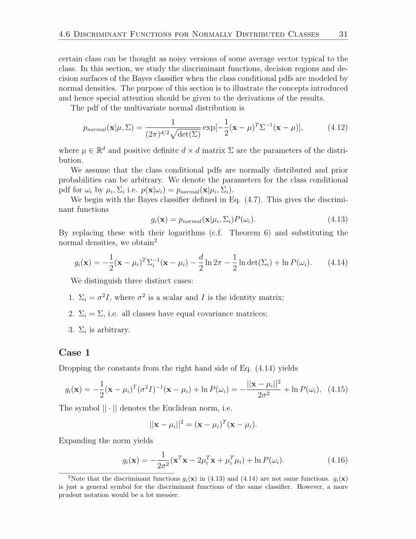
Decision regions in the case 1 are illustrated in Figure 4.3 which is figure 2.10from Duda, Hart and Stork.
Figure 4.3: Case 1
An important special case of the discriminant functions (4.15) is obtained whenP (ωi) = 1
cfor all i. Then x is assigned to the class with the mean vector closest to
x:. This is called minimum distance classifier. It is a linear classifier as a specialcase of a linear classifier.
Case 2
We obtain a linear classifier even if the features are dependent, but the covariancematrices for all classes are equal (i.e. Σi = Σ). It can be represented by thediscriminant functions
gi(x) = wTi x + wi0, (4.18)
wherewi = Σ−1µi
and
wi0 = −1
2µTi Σ−1µi + lnP (ωi).
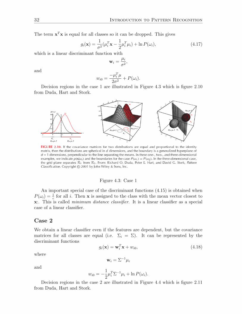
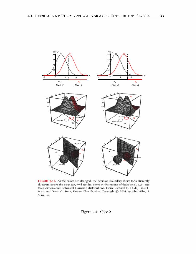
Decision regions in the case 2 are illustrated in Figure 4.4 which is figure 2.11from Duda, Hart and Stork.
4.6 Discriminant Functions for Normally Distributed Classes 33
Figure 4.4: Case 2
34 Introduction to Pattern Recognition
Case 3
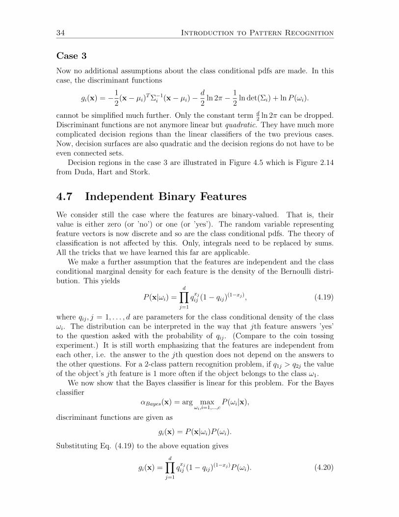
Now no additional assumptions about the class conditional pdfs are made. In thiscase, the discriminant functions
gi(x) = −1
2(x− µi)TΣ−1i (x− µi)−
d
2ln 2π − 1
2ln det(Σi) + lnP (ωi).
cannot be simplified much further. Only the constant term d2
ln 2π can be dropped.Discriminant functions are not anymore linear but quadratic. They have much morecomplicated decision regions than the linear classifiers of the two previous cases.Now, decision surfaces are also quadratic and the decision regions do not have to beeven connected sets.
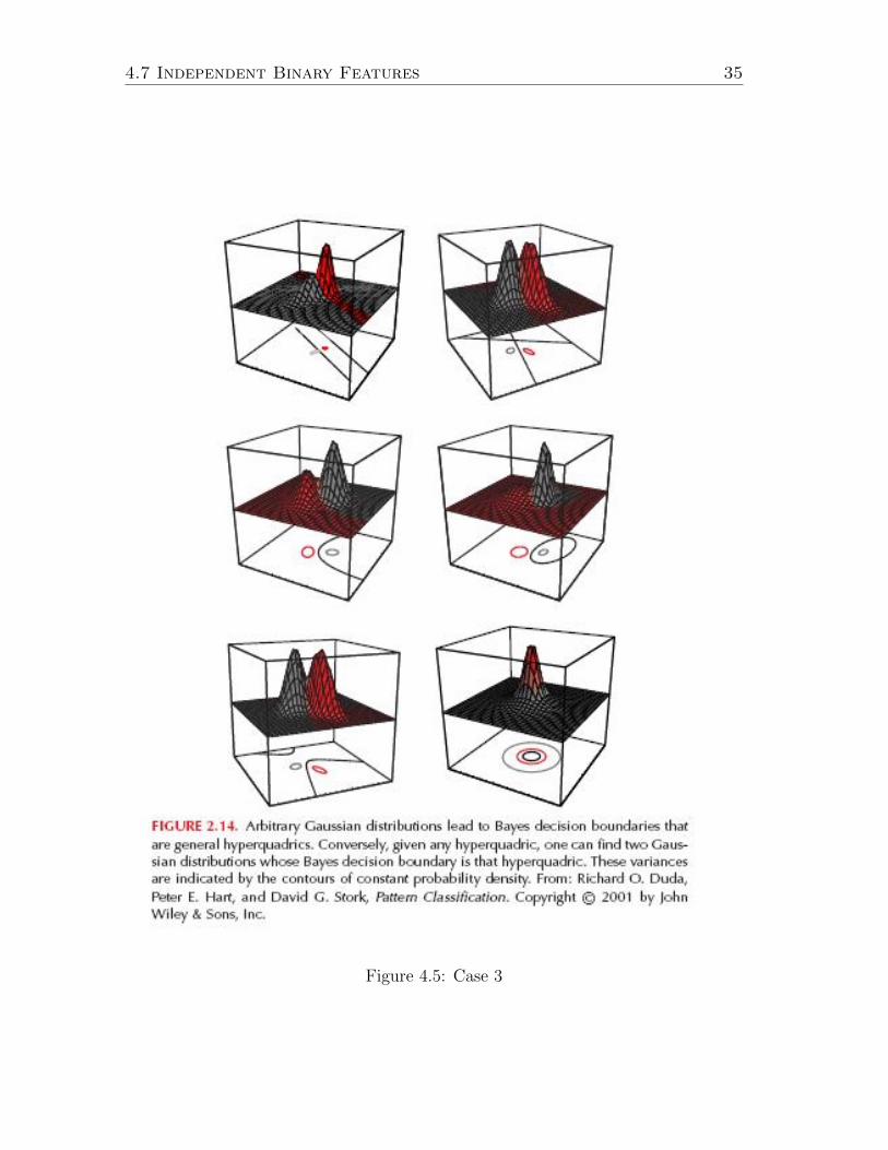
Decision regions in the case 3 are illustrated in Figure 4.5 which is Figure 2.14from Duda, Hart and Stork.
4.7 Independent Binary Features
We consider still the case where the features are binary-valued. That is, theirvalue is either zero (or ’no’) or one (or ’yes’). The random variable representingfeature vectors is now discrete and so are the class conditional pdfs. The theory ofclassification is not affected by this. Only, integrals need to be replaced by sums.All the tricks that we have learned this far are applicable.
We make a further assumption that the features are independent and the classconditional marginal density for each feature is the density of the Bernoulli distri-bution. This yields
P (x|ωi) =d∏j=1
qxjij (1− qij)(1−xj), (4.19)
where qij, j = 1, . . . , d are parameters for the class conditional density of the classωi. The distribution can be interpreted in the way that jth feature answers ’yes’to the question asked with the probability of qij. (Compare to the coin tossingexperiment.) It is still worth emphasizing that the features are independent fromeach other, i.e. the answer to the jth question does not depend on the answers tothe other questions. For a 2-class pattern recognition problem, if q1j > q2j the valueof the object’s jth feature is 1 more often if the object belongs to the class ω1.
We now show that the Bayes classifier is linear for this problem. For the Bayesclassifier
αBayes(x) = arg maxωi,i=1,...,c
P (ωi|x),
discriminant functions are given as
gi(x) = P (x|ωi)P (ωi).
Substituting Eq. (4.19) to the above equation gives
gi(x) =d∏j=1
qxjij (1− qij)(1−xj)P (ωi). (4.20)
4.7 Independent Binary Features 35
Figure 4.5: Case 3
36 Introduction to Pattern Recognition
Replacing the right hand side by its logarithm and simplifying give
gi(x) =d∑j=1
[xj ln qij + ln(1− qij)− xj ln(1− qij)] + lnP (ωi). (4.21)
These are linear discriminant functions
gi(x) = wTi x + wi0 =
d∑j=1
wijxj + wi0,
wherewij = ln
qij1− qij
,
and
wi0 =d∑j=1
ln(1− qij) + lnP (ωj).
In the case of just two classes, the discriminant function is
g(x) = g1(x)− g2(x) =d∑j=1
lnq1j(1− q2j)(1− q1j)q2j
xj +d∑j=1
ln(1− q1j)(1− q2j)
+ lnP (ω1)
P (ω2).
We will end this section (and chapter) by studying how the value of the clas-sification error behaves when we add more and more independent features to theclassification problem. This is somewhat more pleasant in the discrete case when wedo not need to evaluate integrals numerically. However, in order to make compu-tations feasible for large d, we must make some additional simplifying assumptions.Here the results are more important than their derivation and we will keep deriva-tions as brief as possible.
The classification error is
E(αBayes) = 1−∑x
maxP (x|ωi)P (ωi), (4.22)
where x is summed over all d-bit binary vectors. Again, the greater the probabilityof the most probable class the smaller the classification error. Consider the 2-classcase. We model the classes using Binomial densities, that is qij = qi for all featuresj, and
P (x|ωi) = P (∑
xj = k|qi) = qki (1− qi)d−k, i = 1, 2,
where k is the number of 1s in the feature vector x. Let us still assume that theprior probabilities are equal to 0.5 and q1 > q2. The class of the feature vector isdecided by how many 1s it contains. The Bayes classifier is linear and it classifies xto ω1 if the number of 1s in x exceeds a certain threshold t. The threshold t can becomputed from (4.21). The classification error is
E(αBayes) = 1−∑x:k≤t
0.5qk2(1− q2)d−k +∑x:k>t
0.5qk1(1− q1)d−k
= 1−t∑
k=0
0.5d!
k!(d− k)!qk2(1− q2)d−k +
d∑k=t+1
0.5d!
k!(d− k)!qk1(1− q1)d−k.
4.7 Independent Binary Features 37
Note that the trick here is that we can treat all x with certain number of 1s (denotedby k) equally. Since there are many fewer different k than there are different x, thecomputations are much simplified.
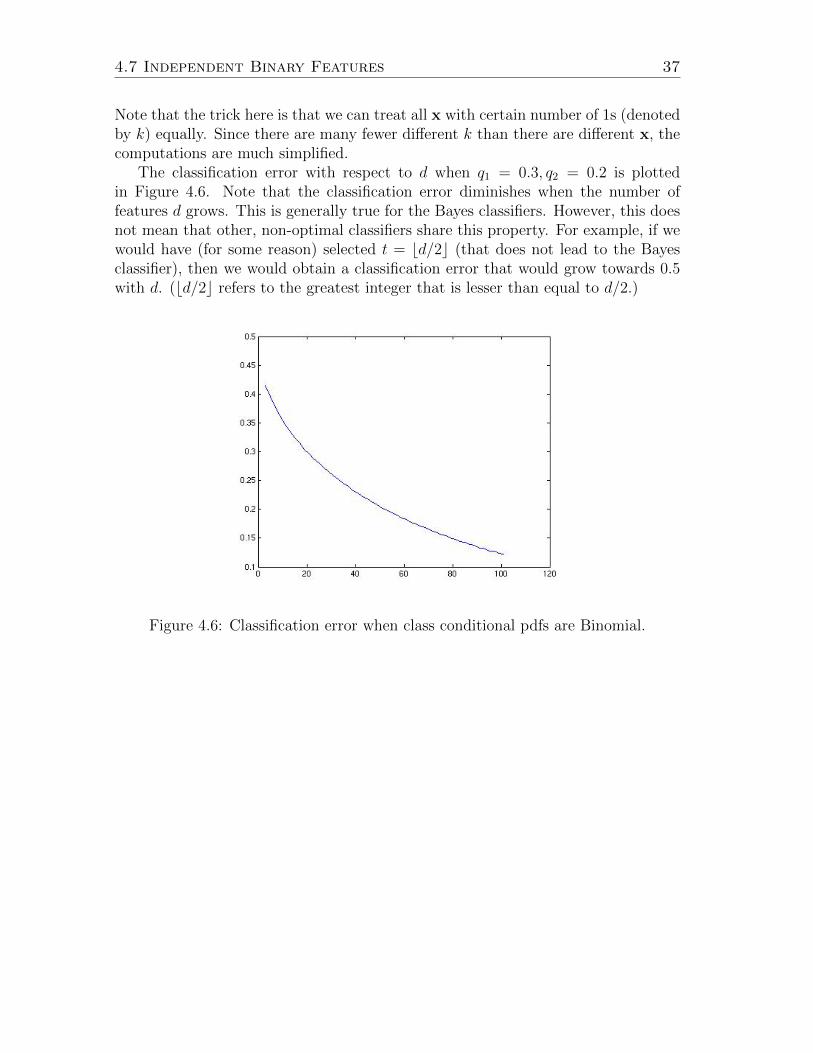
The classification error with respect to d when q1 = 0.3, q2 = 0.2 is plottedin Figure 4.6. Note that the classification error diminishes when the number offeatures d grows. This is generally true for the Bayes classifiers. However, this doesnot mean that other, non-optimal classifiers share this property. For example, if wewould have (for some reason) selected t = bd/2c (that does not lead to the Bayesclassifier), then we would obtain a classification error that would grow towards 0.5with d. (bd/2c refers to the greatest integer that is lesser than equal to d/2.)
Figure 4.6: Classification error when class conditional pdfs are Binomial.

38 Introduction to Pattern Recognition
Chapter 5
Supervised Learning of the BayesClassifier
5.1 Supervised Learning and the Bayes Classifier
In the previous chapter, we assumed that the class conditional pdfs p(x|ωi) and theprior probabilities P (ωi) were known. In practice, this is never the case. Designing aclassifier based on the Bayes decision theory implies learning of the class conditionalpdfs and priors. In this chapter, we study supervised learning of class conditionalpdfs.
For supervised learning we need training samples. As we have defined in Chapter2, training samples are feature vectors for which the correct classes are known. Werefer to the set of training samples as training data or as training set. In the trainingset there are feature vectors from each class ω1, . . . , ωc. We can re-arrange trainingsamples based on their classes: Training samples from the class ωi are denoted by
Di = {xi1, . . . ,xini},
where ni is the number of training samples from the class ωi. We assume thatthe training samples in the sets Di are occurrences of the independent randomvariables. (That is: they were measured from different objects.) Further, theserandom variables are assumed to be distributed according to p(x|ωi). In short, wesay that Di is independent and identically distributed (i.i.d.).
The training data may be collected in two distinct ways. These are meaningfulwhen we need to learn the prior probabilities. In mixture sampling, a set of objectsare randomly selected, their feature vectors are computed and then the objects arehand-classified to the most appropriate classes. (This results pairs consisting of afeature vector and the class of the feature vector, but these pairs can be re-arrangedto obtain representation as above for the training data.) In separate sampling, thetraining data for each class is collected separately. For the classifier training, thedifference of these two sampling techniques is that based on the mixed sampling wecan deduce the priors P (ω1), . . . , P (ωc) as
P (ωi) =ni∑cj=1 nj
. (5.1)
40 Introduction to Pattern Recognition
On the other hand, the prior probabilities cannot be deduced based on the separatesampling, and in this case, it is most reasonable to assume that they are known.
The estimation of class conditional pdfs is more difficult. We need now to esti-mate a function p(x|ωi) based on a finite number of training samples. Next sectionsare dedicated to different approaches to estimate the class conditional pdfs.
5.2 Parametric Estimation of Pdfs
5.2.1 Idea of Parameter Estimation
We study first an approach where the estimation of the class conditional pdfs p(x|ωi)is reduced to the estimation of the parameter vector θi. To do this we must assumethat p(x|ωi) belongs to some family of parametric distributions. For example, wecan assume that p(x|ωi) is a normal density with unknown parameters θi = (µi,Σi).Of course, then it is necessary to justify the choice of the parametric family. Goodjustifications are grounded e.g. on physical properties of the sensing equipmentand/or on properties of the feature extractor.
We denote
p(x|ωi) = p(x|ωi, θi),
where the class ωi defines the parametric family, and the parameter vector θi definesthe member of that parametric family. We emphasize that the parametric familiesdo not need to be same for all classes. For example, the class ω1 can be normallydistributed whereas ω2 is distributed according to the Cauchy distribution. Dueto independence of the training samples, the parameter vectors can be estimatedseparately for each class. The aim is now to estimate the value of the parametervector θi based on the training samples
Di = {xi1, . . . ,xini}.
5.2.2 Maximum Likelihood Estimation
We momentarily drop the indices describing the classes to simplify the notation.The aim is to estimate the value of the parameter vector θ based on the trainingsamples D = {x1, . . . ,xn}. We assume that the training samples are occurrences ofi.i.d. random variables distributed according to the density p(x|θ).
The maximum likelihood estimate or the ML estimate θ maximizes the probabilityof the training data with respect to θ. Due to the i.i.d. assumption, the probabilityof D is
p(D|θ) =n∏i=1
p(xi|θ).
Hence
θ = arg maxn∏i=1
p(xi|θ). (5.2)
5.2 Parametric Estimation of Pdfs 41
The function p(D|θ) - when thought as a function of θ - is termed the likelihoodfunction.
Often it is more convenient to work with the logarithm of the likelihood functionthan with the likelihood function itself. The logarithm is an increasing function andtherefore we can safely replace the likelihood function with its logarithm withoutaffecting the maximization result. Hence,
θ = arg maxn∑i=1
ln p(xi|θ). (5.3)
The function ln p(D|θ) =∑n
i=1 ln p(xi|θ) is called the log-likelihood function.
5.2.3 Finding ML-estimate
A pleasant feature of the ML-estimate is that we can find it, or at least searchfor it, numerically. In some important cases, the ML-estimate can be determinedanalytically. This can be done with a following procedure:
1. Derive the gradient of the likelihood function or the log-likelihood function.
2. Solve the zeros of the gradient and search also all the other critical points ofthe (log)-likelihood function. (e.g. the points where at least one of the partialderivatives of the function are not defined are critical in addition to the pointswhere gradient is zero.)
3. Evaluate the (log)-likelihood function at the critical points and select the crit-ical point with the highest likelihood value as the estimate.
A word of warning: the ML-estimate does not necessarily exist for all distribu-tions, for example the likelihood function could grow without limit. However, theML-estimates exist for simple parametric families.
5.2.4 ML-estimates for the Normal Density
We derive the ML-estimates for the normal density
p(x|θ) =1
(2π)d/2√
det(Σ)exp[−1
2(x− µ)TΣ−1(x− µ)].
Consider first the mean vector, i.e. θ = µ. The covariance matrix Σ is assumedto be known and fixed. (We will see that fixing the covariance will not affect theestimate for mean.) The log-likelihood is
l(θ) =n∑i=1
ln p(xi|µ) = −n∑i=1
0.5(ln[(2π)d/2 det(Σ)] + (xi − µ)TΣ−1(xi − µ)).
42 Introduction to Pattern Recognition
Its gradient is
∇l(µ) = −n∑i=1
Σ−1(xi − µ).
Set ∇l(µ) = 0. The matrix Σ is non-singular, and therefore Σ−1 is non-singular.This implies that ∇l(µ) = 0 has a unique solution. The solution is
µ =1
n
n∑i=1
xi. (5.4)
It is easy to see that this is (the only) local maximum of the log-likelihood function,and therefore it is the ML-estimate. Note that in this case, the ML-estimate is thesample mean of D. As we already hinted, the exact knowledge of the covariance wasnot necessary for obtaining the ML-estimate for the mean. Hence, the result holdseven if both µ and Σ were unknown.
The derivation of the ML-estimate for the covariance matrix is more complicated.Hence, we will skip it and just present the result of the derivation. The ML -estimateis
Σ =1
n
n∑i=1
(xi − µ)(xi − µ)T , (5.5)
where µ is the ML estimate for µ defined in Eq. (5.4).
A numeric example:
x_1 x_2 x_3 x_4 x_5
13 -115 119 33 -19
29 119 -4 17 73
mu = 6.2000
46.8000
sigma = 5762.6 -3212.2
-3212.2 1937.0
5.2.5 Properties of ML-Estimate
There exist variety of methods for the parameter estimation. Therefore, it is impor-tant to know some basic properties of the ML-estimates. It is a favourable propertythat the ML-estimate can be sought for numerically. In addition, it has some pleas-ing theoretical properties, which we will briefly describe next.
The ML-estimates are asymptotically unbiased. Less formally, this means thatthey give the correct result on average provided that there are infinitely many train-ing samples available. To be more precise, the expected value of the ML-estimate
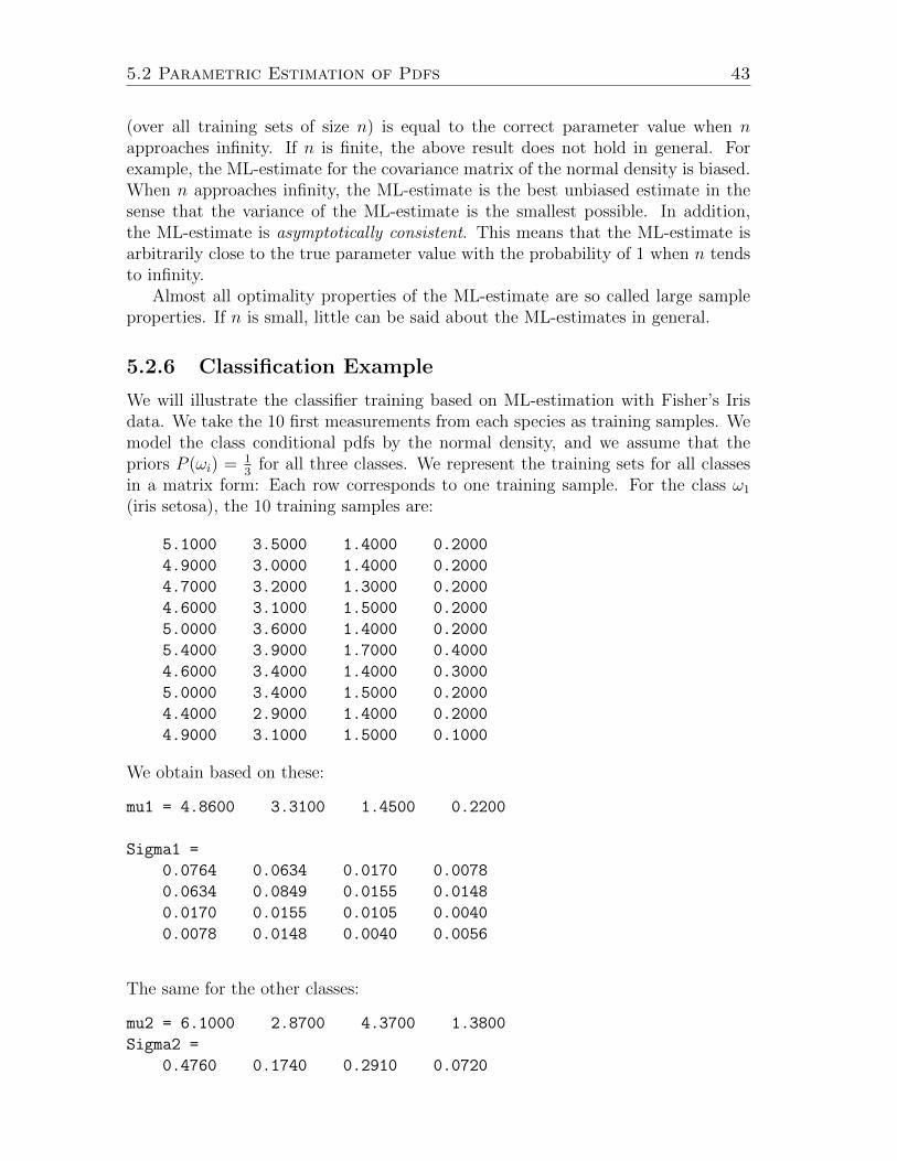
5.2 Parametric Estimation of Pdfs 43
(over all training sets of size n) is equal to the correct parameter value when napproaches infinity. If n is finite, the above result does not hold in general. Forexample, the ML-estimate for the covariance matrix of the normal density is biased.When n approaches infinity, the ML-estimate is the best unbiased estimate in thesense that the variance of the ML-estimate is the smallest possible. In addition,the ML-estimate is asymptotically consistent. This means that the ML-estimate isarbitrarily close to the true parameter value with the probability of 1 when n tendsto infinity.
Almost all optimality properties of the ML-estimate are so called large sampleproperties. If n is small, little can be said about the ML-estimates in general.
5.2.6 Classification Example
We will illustrate the classifier training based on ML-estimation with Fisher’s Irisdata. We take the 10 first measurements from each species as training samples. Wemodel the class conditional pdfs by the normal density, and we assume that thepriors P (ωi) = 1
3for all three classes. We represent the training sets for all classes
in a matrix form: Each row corresponds to one training sample. For the class ω1
(iris setosa), the 10 training samples are:
5.1000 3.5000 1.4000 0.2000
4.9000 3.0000 1.4000 0.2000
4.7000 3.2000 1.3000 0.2000
4.6000 3.1000 1.5000 0.2000
5.0000 3.6000 1.4000 0.2000
5.4000 3.9000 1.7000 0.4000
4.6000 3.4000 1.4000 0.3000
5.0000 3.4000 1.5000 0.2000
4.4000 2.9000 1.4000 0.2000
4.9000 3.1000 1.5000 0.1000
We obtain based on these:
mu1 = 4.8600 3.3100 1.4500 0.2200
Sigma1 =
0.0764 0.0634 0.0170 0.0078
0.0634 0.0849 0.0155 0.0148
0.0170 0.0155 0.0105 0.0040
0.0078 0.0148 0.0040 0.0056
The same for the other classes:
mu2 = 6.1000 2.8700 4.3700 1.3800
Sigma2 =
0.4760 0.1740 0.2910 0.0720
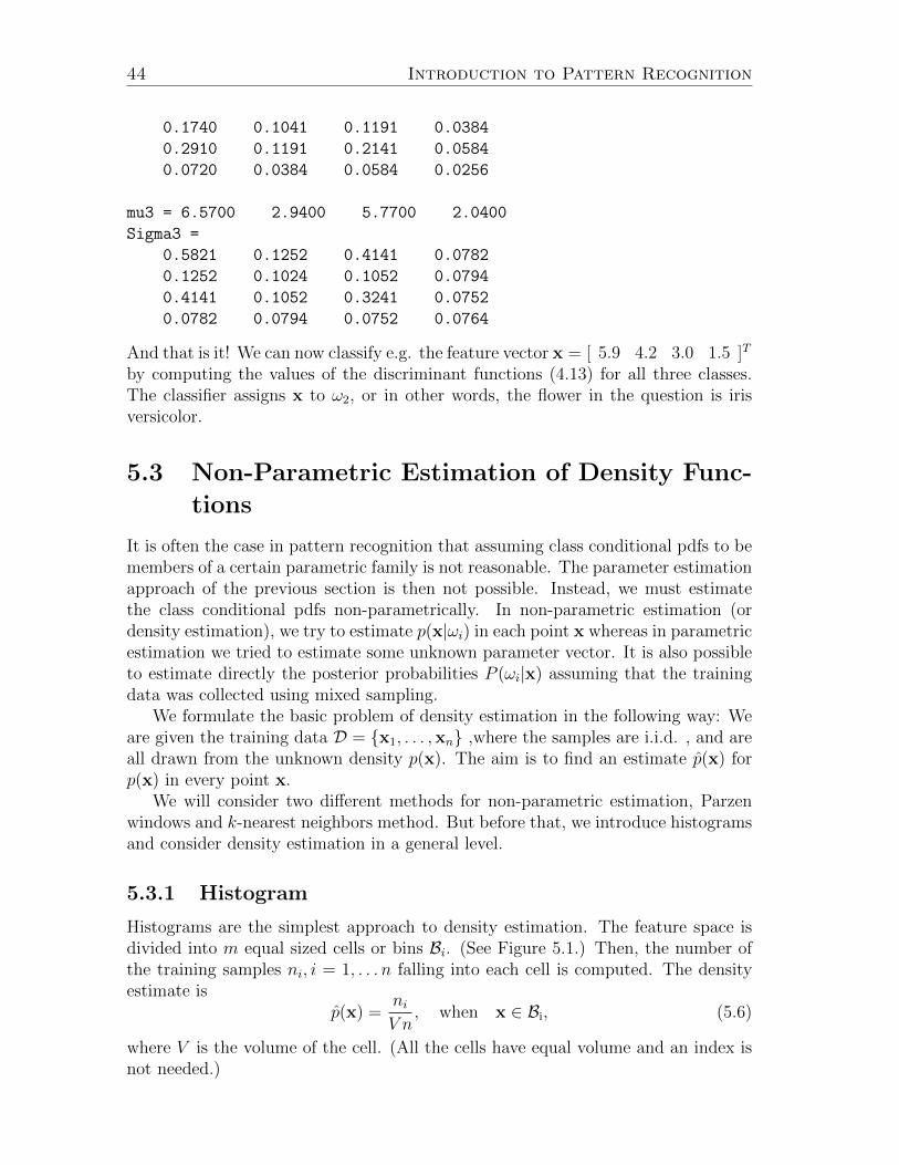
44 Introduction to Pattern Recognition
0.1740 0.1041 0.1191 0.0384
0.2910 0.1191 0.2141 0.0584
0.0720 0.0384 0.0584 0.0256
mu3 = 6.5700 2.9400 5.7700 2.0400
Sigma3 =
0.5821 0.1252 0.4141 0.0782
0.1252 0.1024 0.1052 0.0794
0.4141 0.1052 0.3241 0.0752
0.0782 0.0794 0.0752 0.0764
And that is it! We can now classify e.g. the feature vector x = [ 5.9 4.2 3.0 1.5 ]T
by computing the values of the discriminant functions (4.13) for all three classes.The classifier assigns x to ω2, or in other words, the flower in the question is irisversicolor.
5.3 Non-Parametric Estimation of Density Func-
tions
It is often the case in pattern recognition that assuming class conditional pdfs to bemembers of a certain parametric family is not reasonable. The parameter estimationapproach of the previous section is then not possible. Instead, we must estimatethe class conditional pdfs non-parametrically. In non-parametric estimation (ordensity estimation), we try to estimate p(x|ωi) in each point x whereas in parametricestimation we tried to estimate some unknown parameter vector. It is also possibleto estimate directly the posterior probabilities P (ωi|x) assuming that the trainingdata was collected using mixed sampling.
We formulate the basic problem of density estimation in the following way: Weare given the training data D = {x1, . . . ,xn} ,where the samples are i.i.d. , and areall drawn from the unknown density p(x). The aim is to find an estimate p(x) forp(x) in every point x.
We will consider two different methods for non-parametric estimation, Parzenwindows and k-nearest neighbors method. But before that, we introduce histogramsand consider density estimation in a general level.
5.3.1 Histogram
Histograms are the simplest approach to density estimation. The feature space isdivided into m equal sized cells or bins Bi. (See Figure 5.1.) Then, the number ofthe training samples ni, i = 1, . . . n falling into each cell is computed. The densityestimate is
p(x) =niV n
, when x ∈ Bi, (5.6)
where V is the volume of the cell. (All the cells have equal volume and an index isnot needed.)
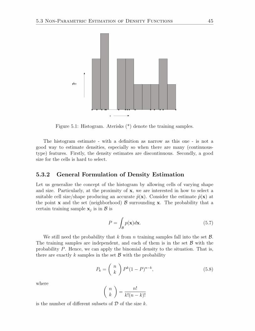
5.3 Non-Parametric Estimation of Density Functions 45
Figure 5.1: Histogram. Aterisks (*) denote the training samples.
The histogram estimate - with a definition as narrow as this one - is not agood way to estimate densities, especially so when there are many (continuous-type) features. Firstly, the density estimates are discontinuous. Secondly, a goodsize for the cells is hard to select.
5.3.2 General Formulation of Density Estimation
Let us generalize the concept of the histogram by allowing cells of varying shapeand size. Particularly, at the proximity of x, we are interested in how to select asuitable cell size/shape producing an accurate p(x). Consider the estimate p(x) atthe point x and the set (neighborhood) B surrounding x. The probability that acertain training sample xj is in B is
P =
∫Bp(x)dx. (5.7)
We still need the probability that k from n training samples fall into the set B.The training samples are independent, and each of them is in the set B with theprobability P . Hence, we can apply the binomial density to the situation. That is,there are exactly k samples in the set B with the probability
Pk =
(nk
)P k(1− P )n−k, (5.8)
where (nk
)=
n!
k!(n− k)!
is the number of different subsets of D of the size k.
46 Introduction to Pattern Recognition
Based on the Binomial theorem, we obtain the expected value of k. It is
E[k] =n∑k=0
kPk =n∑k=1
(n− 1k − 1
)P k−1(1− P )n−knP = nP. (5.9)
(We have skipped some algebra.) Now, we substitute E[k] by the observed numberk of training samples falling into B. We obtain an estimate for P :
P = k/n. (5.10)
If p(x) is continuous and B is small enough,∫Bp(x)dx ' p(x)V,
where V is the volume of B. This gives the estimate (or an interpretation for theestimate)
p(x) =k
nV'∫B p(x)dx∫B dx
. (5.11)
We can draw the following conclusions:
• The obtained density estimate is a space averaged version of the true density.The smaller the volume V the more accurate the estimate is. However, if n isfixed, diminishing V will lead sooner or later to B which does not contain anytraining samples and the density estimate will become useless.
• In more general level two fact need to be accepted. 1) The density estimate isalways a space averaged version of the true density. 2) The estimate k is onlyan estimate of nP when n is finite.
The principal question is how to select B and V . Let us assume that we haveunlimited number of training data. We can then approach this problem in thefollowing manner: To estimate p(x), we form a series of cells B1,B2, . . . containingx. The cell B1 is used when we have just one training sample, the cell B1 is usedwhen we have two training samples and so-forth. The volume of Bn is denoted byVn and the number of training samples falling into Bn is denoted by kn. The densityestimate based on these is
pn(x) =knnVn
.
If we want thatlimn→∞
pn(x) = p(x)
then three conditions must be fulfilled
1. limn→∞ Vn = 0
2. limn→∞ kn =∞
5.4 Parzen Windows 47
3. limn→∞ kn/n = 0.
The conditions may seem rather abstract but they are in fact natural. The firstcondition assures us that the space averaged pn(x) will converge to p(x) if thereare enough training samples. The second one assures us that the frequency ratiokn/n will be a good enough estimate for P . The third one states that the numberof samples falling to a region Bn is always a negligibly small portion of the totalnumber of samples. This is required if pn(x) is to converge at all.
How to guarantee the conditions in the limit of unlimited number of trainingdata? There are two alternatives. We may fix Vn and estimate kn in the best waypossible. Or we can fix kn and estimate Vn. The precise definition of Bn is notnecessary in either alternatives (though it may be implied.)
The optimality results about the density estimators are necessarily of asymptoticnature. Rosenblatt showed already in 1956 that in the continuous case densityestimates based on finite n are necessarily biased.
5.4 Parzen Windows
5.4.1 From Histograms to Parzen Windows
As an introduction to Parzen windows, we consider a certain generalization of thehistogram. Assume that the region Bn is a d-dimensional hypercube. If hn is thelength of the side of the hypercube, its volume is given by Vn = hdn. We define still afunction that receives value 1 inside the hypercube centered at the origin, and value0 outside the hypercube:
ϕ(u) =
{1 if |uj| ≤ 1/20 otherwise
(5.12)
It follows that ϕ((x−xi)/hn) = 1 if xi falls in the hypercube of volume Vn centeredat x. And ϕ((x − xi)/hn) = 0 otherwise. The number of training samples in thishypercube is therefore given by
kn =n∑i=1
ϕ(x− xihn
).
This leads to the density estimate
pn(x) =knnVn
=1
n
n∑i=1
1
Vnϕ(
x− xihn
) (5.13)
Above estimate differs from the histogram defined in section 5.3.1 in that we do notdefine the cells a-priori. Rather the cells are defined only after observing x and theycan also intersect each other for different x.
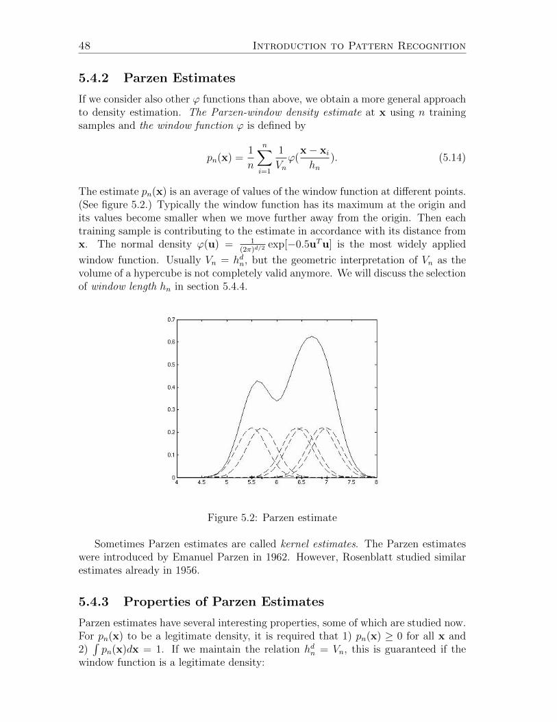
48 Introduction to Pattern Recognition
5.4.2 Parzen Estimates
If we consider also other ϕ functions than above, we obtain a more general approachto density estimation. The Parzen-window density estimate at x using n trainingsamples and the window function ϕ is defined by
pn(x) =1
n
n∑i=1
1
Vnϕ(
x− xihn
). (5.14)
The estimate pn(x) is an average of values of the window function at different points.(See figure 5.2.) Typically the window function has its maximum at the origin andits values become smaller when we move further away from the origin. Then eachtraining sample is contributing to the estimate in accordance with its distance fromx. The normal density ϕ(u) = 1
(2π)d/2exp[−0.5uTu] is the most widely applied
window function. Usually Vn = hdn, but the geometric interpretation of Vn as thevolume of a hypercube is not completely valid anymore. We will discuss the selectionof window length hn in section 5.4.4.
Figure 5.2: Parzen estimate
Sometimes Parzen estimates are called kernel estimates. The Parzen estimateswere introduced by Emanuel Parzen in 1962. However, Rosenblatt studied similarestimates already in 1956.
5.4.3 Properties of Parzen Estimates
Parzen estimates have several interesting properties, some of which are studied now.For pn(x) to be a legitimate density, it is required that 1) pn(x) ≥ 0 for all x and2)∫pn(x)dx = 1. If we maintain the relation hdn = Vn, this is guaranteed if the
window function is a legitimate density:
5.4 Parzen Windows 49
1. ϕ(x) ≥ 0 for all x;
2.∫ϕ(x)dx = 1.
The proof is an exercise.
With an unlimited number of training samples, it is possible to let Vn approachzero, and have pn(x) to converge to p(x) (for example in the point-wise mean-squaresense). For this, it is required that:
1. The density function p must be continuous.
2. The window function must be bounded and a legitimate density.
3. The values of the window function must be negligible at infinity.
4. Vn → 0 when n→∞.
5. nVn →∞ when n→∞.
In addition to the assumptions about the window function and the window length,we needed to make assumptions about the true density. The requirements concerningthe window function are natural and e.g. the normal density is in accordance withthem.
For pattern recognition, these optimality/convergence properties are important,because with these properties we are able to show that the classification error ofa classifier based on Parzen windows tends to the Bayes error when n approachesinfinity. This holds also more generally: When the density estimates converge (ina certain sense) to the true class conditional pdfs, and the prior probabilities areproperly selected, then the error of the resulting classifier tends to the Bayes error.We do not go into detail with the conditions for the convergence, since their propertreatment would require too much effort.
5.4.4 Window Width
The window width satisfying the requirements in the previous paragraph can bechosen as
hn = h1/√n.
In practice, we need to select h1. This is not easy. The choice often is applicationspecific and it is rooted in the properties of the density estimate required by theapplication. If h1 (hn) is too large, then the density estimate pn(x) will be verysmooth and ‘out-of-focus’. If h1 is too small, then the estimate pn(x) will be justsuperposition of n sharp pulses centered at training samples, i.e. an erratic andnoisy estimate of the true density.
50 Introduction to Pattern Recognition
5.4.5 Parzen Classifiers
It is straight-forward to apply Parzen estimates to the classification problems. Foreach class we have the training samples D1, . . . ,Dn. Then, if possible, we firstestimate the priors P (ω1), . . . , P (ωc). Thereafter, we estimate the class conditionalpdfs p(·|ωi) based on Parzen windows, and we construct the Bayes classifier basedon the estimates. The hard part is that it is not possible to estimate p(·|ωi) forall possible feature vectors x. For each test point x to be classified, we must firstcompute the Parzen estimate of the each class conditional density, and only afterthat we can classify the test point. The Parzen-classifier can be written simply as
αParzen(x) = arg maxωi,i=1,...,c
P (ωi)1
ni
ni∑j=1
1
hdiϕ(
x− xijhi
), (5.15)
where P (ωi) are the estimates for prior probabilities, xi1, . . . ,xiniare training sam-
ples from ωi, ϕ is the window function (usually the same window function is usedfor all classes), and hi is the window width for the class ωi.
As can be seen based on Eq. (5.15), Parzen classifier demand much more com-putation than the classifiers based on the ML-estimation. Every classification withParzen classifiers requires n evaluations of a pdf, where n is the total number oftraining samples.
Note that by substituting P (ωi) = ni/n in Eq. (5.15), the Parzen classifier canbe rewritten as
αParzen(x) = arg maxωi,i=1,...,c
1
n
ni∑j=1
1
hdiϕ(
x− xijhi
).
5.4.6 Probabilistic Neural Networks
Parzen classification can be also implemented in an neural network configuration.Such implementation is termed Probabilistic neural network (PNN). Then it is as-sumed that the training samples have been normalized to the unit length, i.e.
||xij || = 1.
Also the test point has to be normalized similarly. This is not reasonable in allapplications. We denote the normalized training samples by yi. We further assumethat the window function is the normal density.
A PNN consists of d input units comprising the input layer, n pattern unitscomprising of the pattern layer, and c category units. Each input unit is connectedto each pattern unit. There is a pattern unit for each training sample. Each patternunit is connected to one and only one category unit corresponding the category ofthe training sample. For the normalized test point x, each pattern unit computesthe inner product
neti = yTi x
5.5 k-Nearest Neighbors Classifier 51
and feeds the value exp[(neti − 1)/h2n] to the category unit to which it is connectedto. Each output unit sums up the contributions of the pattern units connected toit and assigns x to the class with the greatest sum. This indeed implements theParzen classifier because
ϕ(x− yihn
) ∝ exp[−(x− yi)T (x− yi)/(2h
2n)] (5.16)
= exp[−(xTx + yTi yi − 2xTyi)/(2h2n)] (5.17)
= exp[(neti − 1)/h2n], (5.18)
where the last equality is due to our normalization assumptions. Notation a(x) ∝b(x) means that a(x) = C · b(x) for some constant C and for all x.
5.5 k-Nearest Neighbors Classifier
5.5.1 kn Nearest Neighbors Density Estimation
With the Parzen classification, the design of the classifier involved selecting windowfunctions and suitable window widths. This is not an easy task. One possibility islet them depend on the training data. With respect to the general formulation of thedensity estimation, this means fixing kn and computing of suitable (small enough)Vn based on the selected kn. To be more precise, we place the center of the cell Bninto the test point x and let the cell grow until it encircles kn training samples toestimate p(x). These kn training samples are kn nearest neighbors of x. Here, kn isa given parameter. The kn nearest neighbor (KNN) density estimate is given by
pn(x) =knnVn
, (5.19)
where Vn is the volume of the smallest possible x centered ball that contains kntraining samples, and n is the total number of training samples. If the true densityis high in the proximity of x, the cell Bn is small and the density estimate is accurate.If the true density is low in the proximity of x, the cell Bn is large and the densityestimate is not that accurate.
Let p(x) be continuous at x. The KNN density estimate converges if
1. kn →∞ when n→∞;
2. kn/n→ 0 when n→∞.
A surprising property of the KNN density estimate is that although it is continuous,its partial derivatives are necessarily not continuous. Typically, KNN density esti-mates are quite ’spiky’ and the density estimates by Parzen windows more smooth.
It is also possible to estimate posterior probabilities P (ωi|x) directly with theKNN method. This leads to more interesting result than in the case of Parzenwindows. We assume that the training samples D1, . . . ,Dc have been collected bythe mixture sampling. Also, we drop the indices describing the number of training
52 Introduction to Pattern Recognition
samples from all estimates and parameters. This is to avoid confusion in notation.Now, center a cell encircling k training samples at the test point x. The k trainingsamples can be from any class. ki of these belongs to the class ωi. Then, the estimatefor the joint probability of x and ωi is
p(x, ωi) =kinV
.
Using the definition of the conditional densities, we obtain an estimate for the pos-terior probability
P (ωi|x) =p(x, ωi)
p(x)=
p(x, ωi)∑cj=1 p(x, ωj)
=ki∑cj=1 kj
=kik. (5.20)
This posterior probability estimate is maximal for the class with the highest ki andx is assigned to that class. This is the k nearest neighbor (KNN) classification rule.
5.5.2 Nearest Neighbor Rule
We consider first the nearest neighbor (NN) classification, where x is assigned tothe class of its nearest neighbor. That is, k = 1. We can write this rule also as atraditional function:
αnn(x) = arg minωi,i=1,...,c
minj||x− xij ||. (5.21)
It was required that kn →∞ when n→∞ in order to KNN density estimates toconverge to the true density function. With the NN rule, kn = 1 for all n. Therefore,the NN classification rule is not optimal. However, we can show that the error of theNN classifier is at most twice the Bayes error when the number of training samplestends to infinity. More precisely,
E(αbayes) ≤ E(αnn) ≤ E(αbayes)(2−c
c− 1E(αbayes)).
The upper bound is reached when the true class conditional pdfs are identical forall classes.
The rather positive error bound above is a theoretical one. In real life, wedo not have infinite number of training samples and there are no correspondingresults for the case when we have a finite number of training samples. However, theNN classifier is very simple, and in practice it often works well. We explain thisheuristically. Denote the nearest neighbor of the test point x by x∗. Let the class ofx∗ be ω∗. Because we assume that the training samples have been correctly classified,ω∗ maximizes the posterior P (ωi|x∗) with respect to classes ωi, i = 1, . . . , c with highprobability. Then, if x is close to x∗, ω∗ maximizes also the posterior P (ωi|x) withrespect to classes ωi, i = 1, . . . , c with high probability if the posteriors are smoothenough.
We finally consider the geometry of the decision regions of the NN rule. Thedecision region for class ωi is formed by the cells whose points are closer to sometraining sample in Di than any other training sample. This kind of partition of thefeature space is termed Voronoi diagram. See Figure 5.3 due to Duda, Hart andStork.
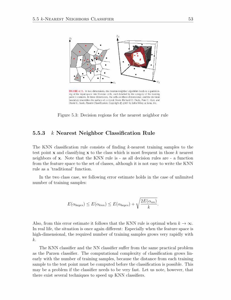
5.5 k-Nearest Neighbors Classifier 53
Figure 5.3: Decision regions for the nearest neighbor rule
5.5.3 k Nearest Neighbor Classification Rule
The KNN classification rule consists of finding k-nearest training samples to thetest point x and classifying x to the class which is most frequent in those k nearestneighbors of x. Note that the KNN rule is - as all decision rules are - a functionfrom the feature space to the set of classes, although it is not easy to write the KNNrule as a ’traditional’ function.
In the two class case, we following error estimate holds in the case of unlimitednumber of training samples:
E(αbayes) ≤ E(αknn) ≤ E(αbayes) +
√2E(αnn)
k.
Also, from this error estimate it follows that the KNN rule is optimal when k →∞.In real life, the situation is once again different: Especially when the feature space ishigh-dimensional, the required number of training samples grows very rapidly withk.
The KNN classifier and the NN classifier suffer from the same practical problemas the Parzen classifier. The computational complexity of classification grows lin-early with the number of training samples, because the distance from each trainingsample to the test point must be computed before the classification is possible. Thismay be a problem if the classifier needs to be very fast. Let us note, however, thatthere exist several techniques to speed up KNN classifiers.
54 Introduction to Pattern Recognition
5.5.4 Metrics
We have assumed until now that the distance between the points a and b in thefeature space (feature vectors) is measured with the Euclidean metric:
L(a,b) = ||a− b|| =
√√√√ d∑i=1
(ai − bi)2.
However, many other distance measures or metrics can be applied. The selectionof a metric obviously affects the KNN classification results. Especially, the scalingof the features has a fundamental effect to the classification results although thistransformation merely accounts to a different choice of units for features.
Formally, a metric is a function L(·, ·) from Rd×Rd to R. For all vectors a,b, c,a metric L must satisfy
1. L(a,b) ≥ 0
2. L(a,b) = 0 if and only if a = b.
3. L(a,b) = L(b, a)
4. L(a,b) + L(b, c) ≥ L(a, c).
The only one of these properties which we occasionally want to sacrifice is theproperty 2. Other properties are important for pattern recognition applications.
Some examples of useful metrics:
• Minkowski metrics:
Lm(a,b) = (d∑i=1
(|ai − bi|m)1/m.
• L-infinity metricL∞(a,b) = max
i|ai − bi|.
• Mahalanobis-distance
LMahalanobis,C(a,b) =√
(a− b)TC−1(a− b),
where C is a given positive definite matrix.
5.6 On Sources of Error
We have mentioned repeatedly in this chapter that the optimality properties of theclassifiers hold only if we have an infinite number of training samples. However, wealways have only a finite number of them. In this section, we discuss the sources oferrors when the number of training samples is finite.
5.6 On Sources of Error 55
Before discussing error sources, it is important to note that in pattern recognitiontwo error types can be distinguished: the training error and the test error. Thetraining error refers to the classification errors for the training samples, i.e., howlarge portion of the training samples is misclassified by the designed classifier. Here,we are not concerned with this error type. The important error type is the the testerror, which describes how large portion of all possible objects are misclassified, andthe discussions below refer to the test error. Note that the Bayes classifier minimizesthe test error when the assumptions made about class conditional pdfs and priorshold. The estimation of the test error is a challenging task, and we will return to theissue in Chapter 7. In particular, the training error, in most cases, underestimatesthe test error.
Before studying the sources of the test error, we recall what kind of inputsdifferent classifiers required for their design. First, all supervised classifiers needtraining samples. Second, the classifiers based on the ML-estimation need knowledgeabout the parametric families of the class conditional pdfs. Parzen classifiers needto be given the window functions and window lengths. For KNN classifiers, we needto select the parameter k.
The Bayes error is a necessary error source of every pattern classification prob-lem. This error can never be reduced without changing the classification problem.If we take into account the whole pattern recognition system, we can change theclassification problem e.g. by adding an extra feature. This can possibly reduce theBayes error.
The second source of classification error with practical classifiers is that theprobabilistic model for the problem is incorrect. This is termed model error. InML-based classification, these are due to having incorrect (parametric) model forclass conditional densities, i.e. the data from the class ωi is not distributed accordingto any of the densities p(·|ωi, θi). In the non-parametric case, we interpret a badselection of window functions, window lengths, or the parameter k as model errors.The model error is more important with the parametric ML-based classifiers thanwith the non-parametric classifiers. This type of error can be reduced by selectiona better probabilistic model for the problem. Again, this is rarely straight-forward.
The third and final error source is the estimation error. This error is due havingonly a finite number of training samples. This error is more pronounced in thenon-parametric case where more training samples are required than with ML-basedclassifiers. In the ML-estimation, the larger the parametric family the lesser themodel error but the greater the estimation error, i.e. there is a trade-off betweenthe model and estimation errors. The estimation error can be reduced by addingmore training samples.
In general, if we add features to the pattern recognition system, we also increasethe estimation error. Further, the required number of training samples grows ex-ponentially with the number of features in the non-parametric case. Hence, addingone more feature to the pattern recognition system might not always be a goodidea. The phenomenon is often termed the curse of dimensionality (the term is dueto Bellman) that refers to the exponential growth of hypervolume as a function ofdimensionality.

56 Introduction to Pattern Recognition
Chapter 6
Linear Discriminant Functions andClassifiers
6.1 Introduction
To this point, we have designed classifiers by estimating the class conditional pdfsand prior probabilities based on training data. Based on the estimated class condi-tional pdfs and prior probabilities, we have then derived the Bayes classifier. Thisway the classifier minimizes the classification error when the estimated pdfs andpriors are close to the true ones. The problem was that the estimation problemsare challenging, and with the finite number of training samples, it is impossible toguarantee the quality of estimates.
In this Chapter, we consider another way to derive the classifier. We assume thatwe know the parametric forms of the discriminant functions in a similar way as withthe ML estimation. The estimation will be formulated as a problem of minimizing acriterion function - again much in a same way than with the ML technique. However,now we are aiming directly to find the discriminant functions without first estimatingthe class conditional pdfs. An example illustrates positive features of this type ofclassifier design: Consider a two-category classification problem, where the classconditional pdfs are normal densities with equal covariances. Then, as stated inSection 4.6, the Bayes classifier is linear, and it can be represented with the followingdiscriminant function:
g(x) = g1(x)− g2(x) = wTx + w0,
wherew = Σ−1(µ1 − µ2)
and
w0 = −1
2(µ1 − µ2)
TΣ−1(µ1 − µ2) + lnP (ω1)− lnP (ω2).
For deriving this discriminant function, it was necessary to estimate 2d+(d2+d)/2+1parameter values. The first term is due to the two mean vectors, the second isdue to the single (symmetric) covariance matrix, and the third one is due to the
58 Introduction to Pattern Recognition
priors which sum to one. Hence, it might be reasonable to estimate directly thediscriminant function, which has only d + 1 parameter values: d of them fromthe weight vector w, and one of them from the threshold weight w0. In addition,the parameterization of the discriminant functions may sometimes be more naturalthan the parameterization of the class conditional pdfs.
The estimation of w and w0 will be performed by minimizing a criterion functionas it was already mentioned. The criterion can be e.g. the number of misclassifiedtraining samples but more often it is some related function. Note, however, thatin this case we will lose the direct contact with the test-error which is much moreimportant quantity than the training error.
6.2 Properties of Linear Classifiers
6.2.1 Linear Classifiers
Recall first how the classifier was defined with the help of discriminant functions.For each class, we had a discriminant function gi, i = 1, . . . , c whose input was afeature vector x. The feature vector x was assigned to ωi if
gi(x) > gj(x)
for all i 6= j. (If gi(x) = gj(x) we can use some arbitrary rule such as classifyingx to ωi if i < j. As with the Bayes classifier, the selection of such a rule bears noimportance.)
A discriminant function is said to be linear if it can written as
gi(x) = wTi x + wi0 =
d∑j=1
wijxj + wi0,
where wi = [wi1, . . . , wid]T is the weight vector and the scalar wi0 is threshold
weight. The classifier relying only on the linear discriminant functions is calledlinear classifier or linear machine.
6.2.2 The Two Class Case
Consider a 2-class classification problem and a linear classifier. The points on thedecision surface satisfy
g1(x) = wT1 x + w10 = wT
2 x + w20 = g2(x).
From this, we get(w1 −w2)
Tx + w10 − w20 = 0.
Denote w = w1 −w2 and w0 = w10 −w20, and represent the classifier with a singlediscriminant function. We obtain the decision surface
R12 = {x|wTx + w0 = 0}. (6.1)
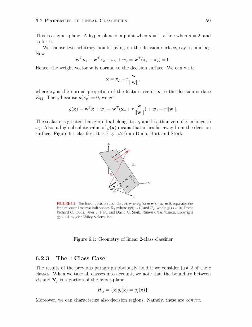
6.2 Properties of Linear Classifiers 59
This is a hyper-plane. A hyper-plane is a point when d = 1, a line when d = 2, andso-forth.
We choose two arbitrary points laying on the decision surface, say x1 and x2.Now
wTx1 −wTx2 − w0 + w0 = wT (x1 − x2) = 0.
Hence, the weight vector w is normal to the decision surface. We can write
x = xp + rw
||w||,
where xp is the normal projection of the feature vector x to the decision surfaceR12. Then, because g(xp) = 0, we get
g(x) = wTx + w0 = wT (xp + rw
||w||) + w0 = r||w||.
The scalar r is greater than zero if x belongs to ω1 and less than zero if x belongs toω2. Also, a high absolute value of g(x) means that x lies far away from the decisionsurface. Figure 6.1 clarifies. It is Fig. 5.2 from Duda, Hart and Stork.
Figure 6.1: Geometry of linear 2-class classifier
6.2.3 The c Class Case
The results of the previous paragraph obviously hold if we consider just 2 of the cclasses. When we take all classes into account, we note that the boundary betweenRi and Rj is a portion of the hyper-plane
Hij = {x|gi(x) = gj(x)}.
Moreover, we can characterize also decision regions. Namely, these are convex.
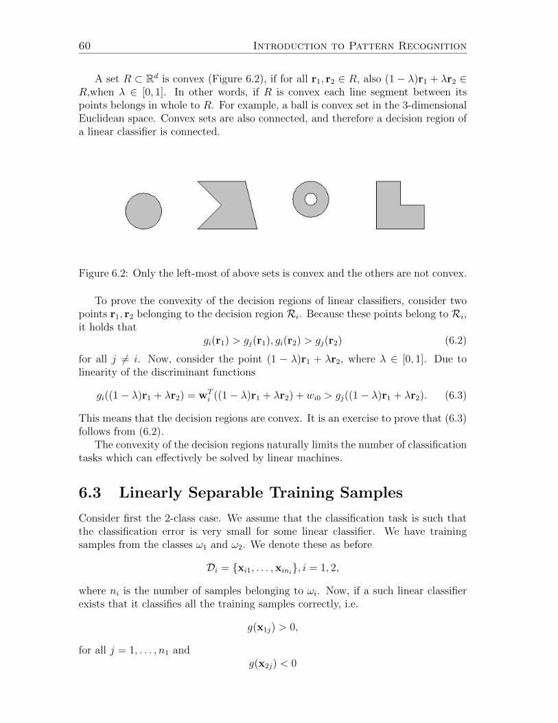
60 Introduction to Pattern Recognition
A set R ⊂ Rd is convex (Figure 6.2), if for all r1, r2 ∈ R, also (1− λ)r1 + λr2 ∈R,when λ ∈ [0, 1]. In other words, if R is convex each line segment between itspoints belongs in whole to R. For example, a ball is convex set in the 3-dimensionalEuclidean space. Convex sets are also connected, and therefore a decision region ofa linear classifier is connected.
Figure 6.2: Only the left-most of above sets is convex and the others are not convex.
To prove the convexity of the decision regions of linear classifiers, consider twopoints r1, r2 belonging to the decision region Ri. Because these points belong to Ri,it holds that
gi(r1) > gj(r1), gi(r2) > gj(r2) (6.2)
for all j 6= i. Now, consider the point (1 − λ)r1 + λr2, where λ ∈ [0, 1]. Due tolinearity of the discriminant functions
gi((1− λ)r1 + λr2) = wTi ((1− λ)r1 + λr2) + wi0 > gj((1− λ)r1 + λr2). (6.3)
This means that the decision regions are convex. It is an exercise to prove that (6.3)follows from (6.2).
The convexity of the decision regions naturally limits the number of classificationtasks which can effectively be solved by linear machines.
6.3 Linearly Separable Training Samples
Consider first the 2-class case. We assume that the classification task is such thatthe classification error is very small for some linear classifier. We have trainingsamples from the classes ω1 and ω2. We denote these as before
Di = {xi1, . . . ,xini}, i = 1, 2,
where ni is the number of samples belonging to ωi. Now, if a such linear classifierexists that it classifies all the training samples correctly, i.e.
g(x1j) > 0,
for all j = 1, . . . , n1 andg(x2j) < 0
6.3 Linearly Separable Training Samples 61
for all j = 1, . . . , n2, we say that the training sets/samples D1 and D2 are linearlyseparable.
Two-class linear classifiers and the above condition can be presented in a morecompact form if we make two modifications to the notation:
1) We form the augmented feature vector y based on x:
y = [1, x1, . . . , xd]T .
Similarly, the augmented weight vector is obtained from w and w0:
a = [w0, w1, . . . , wd]T = [w0,w
T ]T .
Linear discriminant functions can now be written as
g(x) = wTx + w0 = aTy = g(y).
2) We denote by yij the augmented feature vector generated from the trainingsample xij. In the 2-class case, we reduce the two training sets D1,D2 to a singletraining set by simply replacing the training samples from ω2 by their negatives.This because
aTy2j < 0⇔ aT (−y2j) > 0.
Hence, we can forget about ω2, replace its training samples by their negatives, andattach them to the training set for ω1. We denote the resulting training set byD = {y1, . . . ,yn1+n2}. Note that ’replacement by negatives’ must be performedexpressly for augmented feature vectors. (Why?).
Example. Consider the training samples
D1 = {[1, 1]T , [2, 2]T , [2, 1]T}
andD2 = {[1,−1]T , [1,−2]T , [2,−2]T ]
The modified training set is then
D = {[1, 1, 1]T , [1, 2, 2]T , [1, 2, 1]T , [−1,−1, 1]T , [−1,−1, 2]T , [−1,−2, 2]T}.
Given that these two modifications have been performed, we can re-define linearseparability: The training set D is linearly separable if there exists such augmentedweight vector a that
aTyj > 0 (6.4)
for all y1, . . . ,yn1+n2 .If we assume that the training samples are linearly separable, then we can try
to solve the system of inequalities (6.4) to design the linear classifier. One possible
62 Introduction to Pattern Recognition
solution method is introduced in the next section. However, a solution - if exists -is not unique. 1) If we have a solution vector a which is a solution to the system(6.4), then we can always multiply this vector a positive constant to obtain anothersolution. (Remember that the weight vectors were normals to the decision surfaces).2) It is possible to have multiple decision surfaces that separate the training sets.Then, we have many (genuinely different) augmented weight vectors that solve thesystem (6.4).
6.4 Perceptron Criterion and Algorithm in 2-Class
Case
6.4.1 Perceptron Criterion
To find a weight vector a that satisfies
aTyj > 0
for all j, we formulate an optimization problem. We search the minimum argumentof the function
Jp(a) =∑
j:aTyj≤0
−aTyj. (6.5)
The function Jp is termed Perceptron criterion. In other words, we sum the in-ner products of the weight vector a and those training samples that are incorrectlyclassified. The Perceptron criterion is the negative of that sum. Above, we have(implicitly) agreed that augmented feature vectors yj for which aTyj = 0 are in-correctly classified. This assumption is useful in preventing degenerate solutionsa = 01.
The value Jp(a) is always greater than equal to zero. The Perceptron criterionobtains its minimum (that is zero) when a solves the system of inequalities (6.4).(There is also a degenerate case. When a = 0, Jp(a) = 0. However, this obviously isnot the solution we are searching for.) To sum up, we have converted the problemof solving inequalities into an optimization problem.
The criterion∑
j:aTyj≤0−1 would also fulfill the above requirements. However,this criterion function is not continuous which would lead to numerical difficulties.Instead, Jp is continuous.
6.4.2 Perceptron Algorithm
Usually, the analytic (i.e. by paper and pen) minimization of the criterion Jp is notpossible. Therefore, we must rely on numerical techniques to solve the minimizationproblem. The most simple method for the numerical minimization is the steepest
1Note that this assumption/agreement has no effect on the value of the Perceptron criterion.However, it will carry importance when defining the gradient of the Perceptron criterion neededfor deriving the Perceptron algorithm
6.4 Perceptron Criterion and Algorithm in 2-Class Case 63
descent method, which is well applicable here. In the steepest descent method, wechoose an initial value (denoted by a(0)) for a and start updating a little by little tothe direction of the negative gradient of Jp at a(t) at each iteration t = 0, 1, 2, . . ..The idea behind the steepest descent method is the value of any continuous functionf at x decreases most rapidly to the direction of its negative gradient −∇f(x). Thegradient of Jp at a is
∇Jp(a) =∑
j:aTyj≤0
−yj. (6.6)
The update equation is
a(t+ 1) = a(t) + η∑
j:a(t)Tyj≤0
yj,
where t is the iteration counter and the step length η is a parameter. This yieldsthe Perceptron algorithm:
Perceptron algorithmSet t← 0, Initialize a(0), η, ε.while −
∑j:a(t)Tyj≤0 aTyj > ε do
a(t+ 1) = a(t) + η∑
j:a(t)Tyj≤0 yj.Set t← t+ 1
end whileReturn a(t).
Two parameters - in addition to the initial value a(0) - need to be set: Thestopping condition ε and the step length η. Sometimes the step length is called thelearning rate. If training samples indeed are linearly separable, we can set ε to zero.The reason for this is that the Perceptron algorithm converges to the solution ina finite number of steps as long as the training samples are linearly separable. Ifthe training samples are not linearly separable, the Perceptron algorithm does notconverge and it is not a good choice in the linearly non-separable case. The steplength can be set to 1.
Example. We illustrate the Perceptron algorithm by continuing the exampleof Section 6.3 and designing a linear classifier for those training samples. We se-lect a(0) = [1, 1, 1]T . In the first iteration, samples y4,y5, and y6 are incorrectlyclassified. Hence,
a(1) = a(0) + y4 + y5 + y6 = [−2,−3, 6]T .
By a(1), the sample number 3 is misclassified. Hence,
a(2) = a(1) + y3 = [−1,−1, 7]T .
64 Introduction to Pattern Recognition
This is also the final result since all the training samples are now correctly classified.The resulting decision rule is: Classify x to ω1 if g(x) = [−1, 7]x − 1 > 0 to ω2
otherwise. It is staight-forward to determine the decision surface of the classifierbased on the augmented weight vector. The decision surface is a line, because d = 2and the classifier is linear. For the feature vectors x on the decision surface it holdsthat g(x) = 0. The easiest way to draw the decision surface is detect two pointsfrom the surface (two points on a line define uniquely that line). For example, thefeature vectors [−1, 0]T and [6, 1]T lay on the decision surface. Thus we can drawthe decision surface based on these (see 6.3 in the section 6.6).
6.5 Perceptron for Multi-Class Case
We have concentrated only on the design of 2-class linear classifiers up to this point.Now, we would like to design a linear classifier for a c-class problem. We haveaugmented training samples from c classes:
Di = {yi1, . . . ,yini}, i = 1, . . . , c.
We say that these training sets are linearly separable if there exists a linear clas-sifier which classifies all the training samples correctly. The task is to find such(augmented) weight vectors a1, . . . , ac that always when y ∈ Di, it holds that
aTi y > aTj y (6.7)
for all j 6= i. In other words
aTi yik > aTj yik,
for all i = 1, . . . , c, j 6= i and k = 1, . . . , ni. These inequalities can be manipulatedto a 2-class and c · d feature problem by the Kesler’s construction. This is a veryuseful theoretical tool but its use leads to computationally ineffective algorithms.
The Perceptron algorithm for the c-class case is:
c-class Perceptron algorithmSet t← 0, initialize a1(0), . . . , ac(0).while Misclassified training samples exist do
for all misclassified yik doai(t+ 1) = ai(t) + yikaj(t+ 1) = aj(t)− yik if ai(t)
Tyik ≤ aj(t)Tyik
al(t+ 1) = al(t) if ai(t)Tyik > al(t)
TyikSet t← t+ 1
end forend whileReturn a1(t), . . . , ac(t).
6.6 Minimum Squared Error Criterion 65
As in the 2-class case, this algorithm works only if the training samples arelinearly separable.
6.6 Minimum Squared Error Criterion
We still need an algorithm for designing linear classifiers when the training samplesare not linearly separable. We will base the algorithm on the minimum squarederror criterion and will now briefly introduce the criterion in the 2-class case.
We modify the training samples again as in Section 6.3. As a result we have asingle training set of augmented feature vectors. We aim to minimize the criterion:
Js(a) =
n1+n2∑i=1
(aTyi − 1)2. (6.8)
The criterion Js can be written in the matrix-form as
Js(a) = ||Y a− 1||2, (6.9)
where Y is the n1 + n2 × d + 1 matrix consisting of the training samples, and 1 isn1 + n2 component vector consisting of only ones. Precisely
Y =
y1
y2...
yn1+n2
and
1 =
11...1
.This criterion has the unique minimum at
a = (Y TY )−1Y T1. (6.10)
Note that we do not need to assume that Y would be non-singular or square. Theselection of the vector 1 is based on the relation with the Bayes classifier. For moreinformation on this, see section 5.8.3 in Duda, Hart and Stork.
Example Let’s consider the training samples from the example in Section 6.3
66 Introduction to Pattern Recognition
and design a classifier based on these and Minimum Squared Error Criterion. Now
Y =
1 1 11 2 21 2 1−1 −1 1−1 −1 2−1 −2 2
and
1 =[
1 1 1 1 1 1]T.
We can compute the augmented weight vector using Matlab:
>> a = inv(Y’*Y)*Y’*ones(6,1)
a =
0.0000
0.0667
0.6000
The discriminant function is g(x) = [0.0667, 0.6]x. Decision surface can be solved inthe same manner as in the case of Perceptron criterion: points [0, 0]T and [−9, 1]T
lay on the decision surface (see Fig. 6.3).
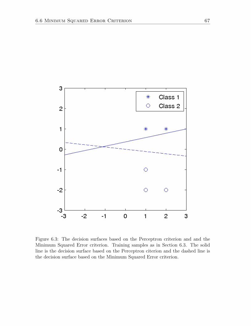
6.6 Minimum Squared Error Criterion 67
Figure 6.3: The decision surfaces based on the Perceptron criterion and and theMinimum Squared Error criterion. Training samples as in Section 6.3. The solidline is the decision surface based on the Perceptron citerion and the dashed line isthe decision surface based on the Minimum Squared Error criterion.

68 Introduction to Pattern Recognition
Chapter 7
Classifier Evaluation
7.1 Estimation of the Probability of the Classifi-
cation Error
It is important to estimate the error probability of the classifier when designingpractical pattern recognition systems. This provides answers to important questionssuch as ’is the system good enough or does it need a further improvement?’ and ’isthe classifier A better than the classifier B?’.
Recall once more that we are interested in the probability that a test point whichdoes not belong to the training set is mis-classified. This was termed test error inSection 5.5. Next, we introduce three ways to estimate the test error.
The training error is the frequency of error for the training data. The trainingerror is a poor and overly optimistic estimate to the test error. For example, thetraining error of the NN-classifiers is automatically zero. This is obviously not truefor the test error. The estimation of the test error by the training error is termedas the resubstitution method.
A much better estimate for the test error is obtained by dividing the trainingdata
D = D1 ∪ D2 ∪ · · · ∪ Dc
into two sets Dtraining and Dtest. We use Dtraining for the training of the classifierand Dtest is solely used to estimate the test error. This method is called the holdoutmethod. It is a good method when we have large number of training samples, andhence a modest decrease in the number of training samples does not essentiallydecrease the quality of the classifier. Note that the division into sets Dtraining andDtest must be randomized. For example, selecting Dtest = D1 is not a good idea.
In the case that we have only a few training samples, it is the best to use somecross-validation method to estimate the test error. The most simple of these isthe leave-one-out method. In the leave-one-out method, we drop a single trainingsample from the training set and design a classifier based on the other trainingsamples. Then, it is studied whether the dropped sample is classified correctly ornot by the designed classifier. This is repeated for all n training samples. The test
70 Introduction to Pattern Recognition
error estimate for the classifier α is the obvious
E(α) =v
n,
where v is the number of misclassified training samples, and n =∑c
i=1 ni is the total
number of training samples. (The hat-notation refers to an estimate, i.e. E(α) isan estimate of the true classification error E(α).) This method yields an accurateestimate for the test error. Its main disadvantage is the computational complexity:to estimate the test error for one classifier, we must design n classifiers.
7.2 Confusion Matrix
It is often worthwhile to study the confusion matrix in addition to the classificationerror. The element sij of the confusion matrix
S =
s11 s12 · · · s1c...
. . ....
sc1 sc2 · · · scc
is the number of test samples that are assigned to the class ωi but whose correctclass would be ωj. The order of indices i, j can be selected also differently, and itvaries from one source reference to another. Hence, it pays off to be attentive. Theconfusion matrix can be estimated by the same methods as the test error.
Based on the confusion matrix, the classification (test) error can be obtained as
E(α) =
∑ci=1
∑cj=1 sij −
∑ci=1 sii∑c
i=1
∑cj=1 sij
.
Based on the confusion matrix, also other important quantities for classifier designcan be computed.
7.3 An Example
Let us illustrate the leave-one-out-method in the case of Fisher’s Iris dataset. Westudy the classification based on ML-estimation, and we assume that the class condi-tional pdfs are Gaussian. The data was collected by separate sampling and thereforewe assume that the prior probabilities for all classes are equal. This data can beloaded into Matlab by
>> load fisheriris
command. (At least, if the Statistics Toolbox is available). There should now bevariables ’meas’ and ’species’ in Matlab. The variable ’meas’ contains the featurevectors from 150 Irises and the variable ’species’ contains the class of each featurevector. The feature vectors numbered from 1 to 50 belong to the class ω1 (iris
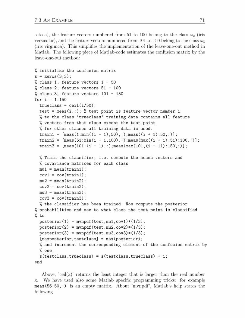
7.3 An Example 71
setosa), the feature vectors numbered from 51 to 100 belong to the class ω2 (irisversicolor), and the feature vectors numbered from 101 to 150 belong to the class ω3
(iris virginica). This simplifies the implementation of the leave-one-out method inMatlab. The following piece of Matlab-code estimates the confusion matrix by theleave-one-out method:
% initialize the confusion matrix
s = zeros(3,3);
% class 1, feature vectors 1 - 50
% class 2, feature vectors 51 - 100
% class 3, feature vectors 101 - 150
for i = 1:150
trueclass = ceil(i/50);
test = meas(i,:); % test point is feature vector number i
% to the class ’trueclass’ training data contains all feature
% vectors from that class except the test point
% for other classes all training data is used.
train1 = [meas(1:min((i - 1),50),:);meas((i + 1):50,:)];
train2 = [meas(51:min(i - 1,100),:);meas(max((i + 1),51):100,:)];
train3 = [meas(101:(i - 1),:);meas(max(101,(i + 1)):150,:)];
% Train the classifier, i.e. compute the means vectors and
% covariance matrices for each class
mu1 = mean(train1);
cov1 = cov(train1);
mu2 = mean(train2);
cov2 = cov(train2);
mu3 = mean(train3);
cov3 = cov(train3);
% the classifier has been trained. Now compute the posterior
% probabilities and see to what class the test point is classified
% to
posterior(1) = mvnpdf(test,mu1,cov1)*(1/3);
posterior(2) = mvnpdf(test,mu2,cov2)*(1/3);
posterior(3) = mvnpdf(test,mu3,cov3)*(1/3);
[maxposterior,testclass] = max(posterior);
% and increment the corresponding element of the confusion matrix by
% one.
s(testclass,trueclass) = s(testclass,trueclass) + 1;
end
Above, ’ceil(x)’ returns the least integer that is larger than the real numberx. We have used also some Matlab specific programming tricks: for examplemeas(56:50,:) is an empty matrix. About ’mvnpdf’, Matlab’s help states thefollowing
72 Introduction to Pattern Recognition
Y = MVNPDF(X,MU,SIGMA) returns the density of the multivariate normal
distribution with mean MU and covariance SIGMA, evaluated at each row
of X.
The confusion matrix is
s =
50 0 0
0 47 1
0 3 49
And the estimate for the test error is accordingly:
E(α) = 4/150 ≈ 0.027.
Chapter 8
Unsupervised Learning andClustering
8.1 Introduction
Until now, we have assumed that we have a set of correctly labeled training sam-ples for training the classifier. These procedures using training samples are partof supervised classification (see Section 2.4). However, in some circumstances it isnecessary to resort to unsupervised classification that is also termed as clustering.These procedures do not use labeled training data. Instead, we have a collection ofunlabeled samples, and we try to classify them based only on the features in data.In other words: there is no explicit teacher. Clearly, clustering is a more difficultproblem than supervised classification. However, there are certain situations whereclustering is either useful or necessary. These include:
1. The collection and classification of training data can be costly and time con-suming. Therefore, it can be impossible to collect a training set. Also, whenthere are very many training samples, it can be that all of these cannot behand-labeled. Then, it is useful to train a supervised classifier with a smallportion of training data and use then clustering procedures to fine tune theclassifier based on the large, unclassified dataset.
2. For data mining, it can be useful to search for natural clusters/groupingsamong the data, and then recognize the clusters.
3. The properties of feature vectors can change over time. Then, supervisedclassification is not reasonable, because sooner or later the test feature vectorswould have completely different properties than the training data had. Forexample, this problem is commonplace in the processing of medical images.
4. The clustering can be useful when searching for good parametric families forthe class conditional densities for the supervised classification.
Above situations only are examples of the situations where clustering is worth-while. There are many more situations requiring clustering.
74 Introduction to Pattern Recognition
8.2 The Clustering Problem
We define the clustering problem more precisely. We have a set of feature vectors
D = {x1, . . . ,xn}.
The task is to place each of these feature vectors into one of the c classes. In otherwords, the task is to find c sets D1, . . . ,Dc so that
c⋃i=1
Di = D
andDj ∩ Di = ∅
for all i 6= j.Naturally, we need some further assumptions for the problem to be sensible.
(An arbitrary division of D into different classes is not likely to be useful.) Here,we assume that we can measure the similarity of any two feature vectors somehow.Then, the task is to maximize the similarity of feature vectors within a class. Forthis, we need to be able to define how similar are the feature vectors belonging tosome set Di.
In the following sections, we will introduce two alternatives for defining howsimilar a certain set of feature vectors is. We have already seen their counterparts insupervised classification. The first one, the k-means clustering, reminds minimumdistance classification. The second one, the expectation maximization algorithm, isrooted on ML-estimates and finite mixture models
8.3 K-means Clustering
8.3.1 K-means Criterion
Recall that the minimum distance classifier assigned a test point to the class withthe nearest mean to the test point. Denote now the number of feature vectors inthe class Di by ni. (We do not know the value of ni yet.).
The problem is that we do not know the mean vectors. Despite of this, definethe similarity of Di as
s(Di) = −∑x∈Di
||x− µi||2,
where µi = 1ni
∑x∈Di
x. We solve the unknown mean vectors by maximizing thesum of similarities of all classes. Equivalently, we can minimize the negative of thissum:
J(D1, . . . ,Dc) =c∑i=1
∑x∈Di
||x− µi||2. (8.1)
This is the k-means criterion.
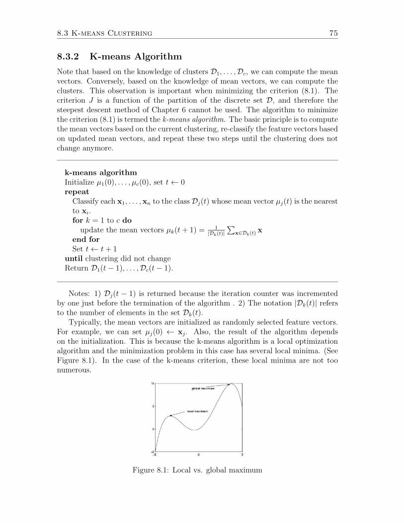
8.3 K-means Clustering 75
8.3.2 K-means Algorithm
Note that based on the knowledge of clusters D1, . . . ,Dc, we can compute the meanvectors. Conversely, based on the knowledge of mean vectors, we can compute theclusters. This observation is important when minimizing the criterion (8.1). Thecriterion J is a function of the partition of the discrete set D, and therefore thesteepest descent method of Chapter 6 cannot be used. The algorithm to minimizethe criterion (8.1) is termed the k-means algorithm. The basic principle is to computethe mean vectors based on the current clustering, re-classify the feature vectors basedon updated mean vectors, and repeat these two steps until the clustering does notchange anymore.
k-means algorithmInitialize µ1(0), . . . , µc(0), set t← 0repeat
Classify each x1, . . . ,xn to the class Dj(t) whose mean vector µj(t) is the nearestto xi.for k = 1 to c do
update the mean vectors µk(t+ 1) = 1|Dk(t)|
∑x∈Dk(t)
xend forSet t← t+ 1
until clustering did not changeReturn D1(t− 1), . . . ,Dc(t− 1).
Notes: 1) Dj(t − 1) is returned because the iteration counter was incrementedby one just before the termination of the algorithm . 2) The notation |Dk(t)| refersto the number of elements in the set Dk(t).
Typically, the mean vectors are initialized as randomly selected feature vectors.For example, we can set µj(0) ← xj. Also, the result of the algorithm dependson the initialization. This is because the k-means algorithm is a local optimizationalgorithm and the minimization problem in this case has several local minima. (SeeFigure 8.1). In the case of the k-means criterion, these local minima are not toonumerous.
Figure 8.1: Local vs. global maximum
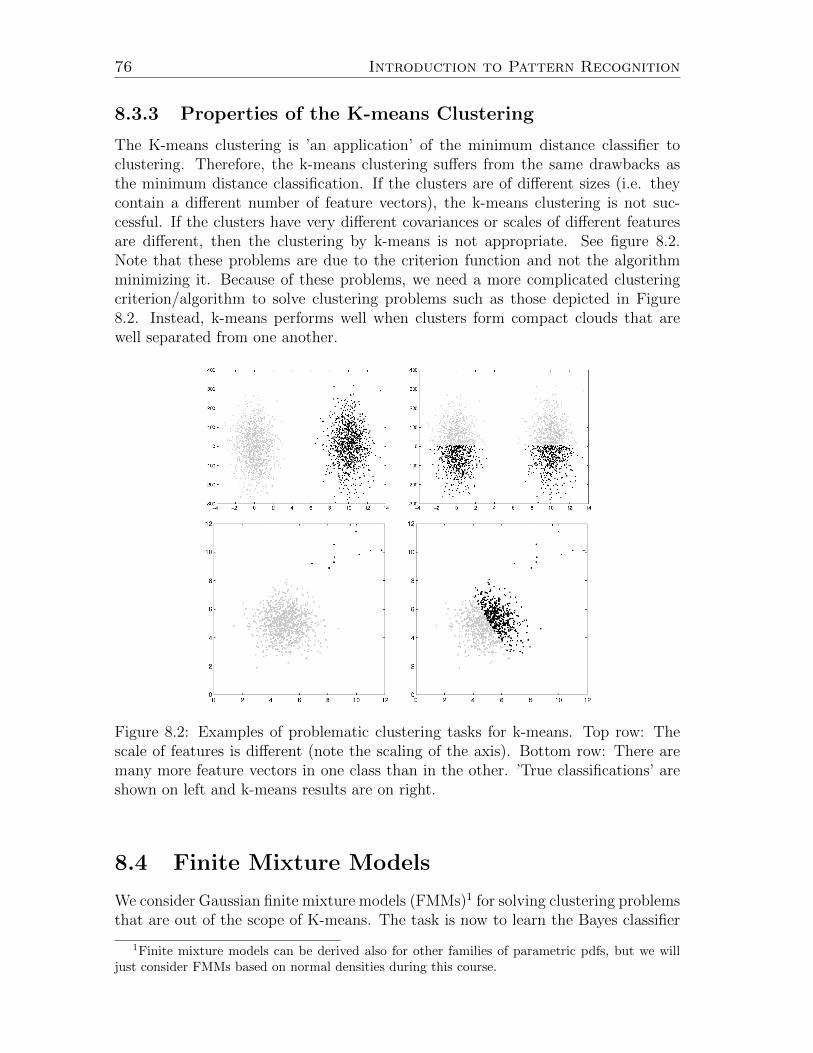
76 Introduction to Pattern Recognition
8.3.3 Properties of the K-means Clustering
The K-means clustering is ’an application’ of the minimum distance classifier toclustering. Therefore, the k-means clustering suffers from the same drawbacks asthe minimum distance classification. If the clusters are of different sizes (i.e. theycontain a different number of feature vectors), the k-means clustering is not suc-cessful. If the clusters have very different covariances or scales of different featuresare different, then the clustering by k-means is not appropriate. See figure 8.2.Note that these problems are due to the criterion function and not the algorithmminimizing it. Because of these problems, we need a more complicated clusteringcriterion/algorithm to solve clustering problems such as those depicted in Figure8.2. Instead, k-means performs well when clusters form compact clouds that arewell separated from one another.
Figure 8.2: Examples of problematic clustering tasks for k-means. Top row: Thescale of features is different (note the scaling of the axis). Bottom row: There aremany more feature vectors in one class than in the other. ’True classifications’ areshown on left and k-means results are on right.
8.4 Finite Mixture Models
We consider Gaussian finite mixture models (FMMs)1 for solving clustering problemsthat are out of the scope of K-means. The task is now to learn the Bayes classifier
1Finite mixture models can be derived also for other families of parametric pdfs, but we willjust consider FMMs based on normal densities during this course.
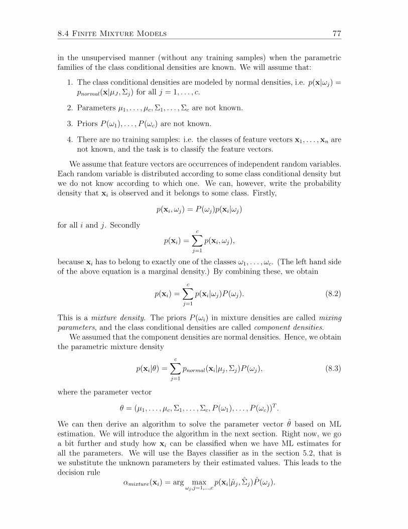
8.4 Finite Mixture Models 77
in the unsupervised manner (without any training samples) when the parametricfamilies of the class conditional densities are known. We will assume that:
1. The class conditional densities are modeled by normal densities, i.e. p(x|ωj) =pnormal(x|µJ ,Σj) for all j = 1, . . . , c.
2. Parameters µ1, . . . , µc,Σ1, . . . ,Σc are not known.
3. Priors P (ω1), . . . , P (ωc) are not known.
4. There are no training samples: i.e. the classes of feature vectors x1, . . . ,xn arenot known, and the task is to classify the feature vectors.
We assume that feature vectors are occurrences of independent random variables.Each random variable is distributed according to some class conditional density butwe do not know according to which one. We can, however, write the probabilitydensity that xi is observed and it belongs to some class. Firstly,
p(xi, ωj) = P (ωj)p(xi|ωj)
for all i and j. Secondly
p(xi) =c∑j=1
p(xi, ωj),
because xi has to belong to exactly one of the classes ω1, . . . , ωc. (The left hand sideof the above equation is a marginal density.) By combining these, we obtain
p(xi) =c∑j=1
p(xi|ωj)P (ωj). (8.2)
This is a mixture density. The priors P (ωi) in mixture densities are called mixingparameters, and the class conditional densities are called component densities.
We assumed that the component densities are normal densities. Hence, we obtainthe parametric mixture density
p(xi|θ) =c∑j=1
pnormal(xi|µj,Σj)P (ωj), (8.3)
where the parameter vector
θ = (µ1, . . . , µc,Σ1, . . . ,Σc, P (ω1), . . . , P (ωc))T .
We can then derive an algorithm to solve the parameter vector θ based on MLestimation. We will introduce the algorithm in the next section. Right now, we goa bit further and study how xi can be classified when we have ML estimates forall the parameters. We will use the Bayes classifier as in the section 5.2, that iswe substitute the unknown parameters by their estimated values. This leads to thedecision rule
αmixture(xi) = arg maxωj ,j=1,...,c
p(xi|µj, Σj)P (ωj).
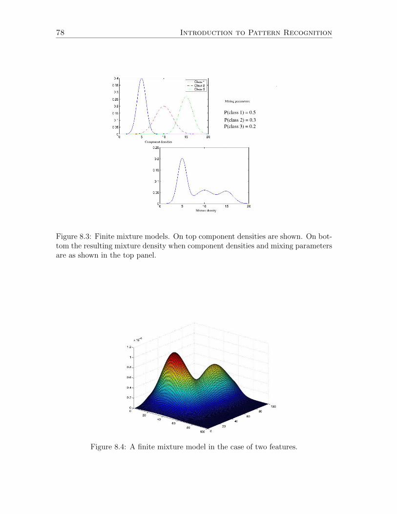
78 Introduction to Pattern Recognition
Figure 8.3: Finite mixture models. On top component densities are shown. On bot-tom the resulting mixture density when component densities and mixing parametersare as shown in the top panel.
Figure 8.4: A finite mixture model in the case of two features.
8.5 EM Algorithm 79
A problem with FMMs is that they are not always identifiable. This means thattwo different parameter vectors θ1 and θ2 may result in exactly the same mixturedensity, i.e.
p(x|θ1) = p(x|θ2)
for all x. However, the classifier derived based on the parameter vector θ1 can stillbe different than the classifier that is based on θ2. And therefore, this is a seriousproblem because the parameter vectors cannot be distuinguished from each otherbased on ML estimation.. Switching problems are special cases of identifiabilityproblems. If we switch the classes ωi and ωj, we end up with exactly the samemixture density as long as component densities for ωi and ωj belong to the sameparametric family. Therefore, the classes must be named (or given interpretation)after the classification. This is problematic, if we are after a completely unsupervisedclassifier.
8.5 EM Algorithm
We return to solving the ML estimation problem. Because x1, . . . ,xn were occur-rences of independent random variables, we can write the likelihood function as
n∏i=1
p(xi|θ) =n∏i=1
c∑j=1
pnormal(xi|µj,Σj)P (ωj).
Maximizing this with respect to the parameter vector θ results in the ML estimateθ. Once again, it is more convenient to deal with the log-likelihood function, i.e.
θ = arg maxθ
n∑i=1
ln[c∑j=1
pnormal(xi|µj,Σj)P (ωj)]. (8.4)
This is a challenging maximization task. (Actually, we are interested in the largestlocal maximum, because the (log)-likelihood function is not bounded from above,see e.g. Duda, Hart, Stork, Chapter 10). However, we can derive a expectation-maximization (EM) algorithm for solving (8.4). We will skip the derivation. Thealgorithm can be given as:
80 Introduction to Pattern Recognition
EM algorithm
1. Initialize µ0j ,Σ
0j , P
0(ωj), set t← 0.
2. (E-step) Compute the posterior probabilities that xi belongs to the class ωj
pt+1ij =
P t(ωj)pnormal(xi|µtj,Σtj)∑c
k=0 Pt(ωk)pnormal(xi|µtk,Σt
k).
3. (M-step) Update the parameter values
P t+1(ωj) = (1/n)∑i
pt+1ij (8.5)
µt+1j =
∑i p
t+1ij xi∑
i pt+1ij
(8.6)
Σt+1j =
∑i p
t+1ij (xi − µt+1
j )(xi − µt+1j )T∑
i pt+1ij
(8.7)
4. Set t← t+ 1.
5. Stop if some convergence criterion is fulfilled, otherwise return to step 2.
In most cases, The EM algorithm finds a local maximum of the likelihood func-tion. However, there are usually several local maxima and hence the final result isstrongly dependent on the initialization.