Sex and performance under competition: Is

there a stereotype threat shadow?1

Diogo Geraldes23 Arno Riedl2 Martin Strobel2

September 2011

Preliminary version. Please do not quote or circulate without permission of the authors.

Abstract

In this paper we experimentally study performance of men and women under

competition, with implicitly and explicitly induced stereotype threats to both

sexes. We use a mathematical task that is perceived as male-dominant and

creates an implicit stereotype threat against woman. We also study conditions

in which we explicitly reinforce or contradict the implicit stereotype threat by

providing appropriate information. We find that despite stereotype threats

against women, both men and women react positively and equally strong to

competitive incentives. When the stereotype threat is explicitly contradicted,

competitive incentives do not have an effect on the performance of both men

and women. Our findings contrast previous results suggesting that men are

more responsive to competition than women. We observe that men and women

react similarly to competition in terms of performance across three different

stereotype threat conditions. Interestingly, we also find that explicit stereotype-

based expectations that contradict the stereotype men and women hold harm

the competitive performance of both sexes.

Keywords: competition, incentives, sexes, stereotype threat

JEL classification: C91; J16

1 We would like to thank for invaluable comments all the participants of the Experimental design seminar

series at Maastricht University, Nordic Conference on BEE 2010 in Helsinki, IMEBE 2011 in Barcelona,

International ESA Conference 2011, TIBER 2011 at Tilburg University and EEA-ESEM 2011 in Oslo.

We are grateful that Thomas Dohmen provided us with his z-tree program for the work task.

2 Maastricht University, Department of Economics – Section AE1

3 Corresponding author. Address: Maastricht University, Department of Economics – Section AE1, P.O.

Box 616, Maastricht 6200 MD, The Netherlands. E-mail: d.geraldes@maastrichtuniversity.nl

1

1. Introduction

A politically, socially and economically important stylized fact about sex1 differences is the

gap in wages and positions at the workplace. In 2006 women earned, on average, 25% less than

men in the 27 European Union countries. In academics, qualified research positions such as

PhD candidates, post-doctoral or assistant professors, associate professors and full professors

are dominated by men. For instance, only 19% of all full professors in the 27 European Union

countries are women.2 Further evidence for the disadvantaged position of women at the

workplace is presented, for example, by Bertrand and Hallock (2001).3

One common explanation for these differences between the sexes at the workplace is

discrimination (e.g., Black and Strahan, 2001). Another one is women’s higher sensitivity to

work-family conflicts and women’s weaker negotiation behavior (e.g., Babcock and Laschever,

2003). An alternative explanation has been suggested by recent studies in experimental

economics: men are more inclined to compete than women. These studies show that even under

tightly controlled and relatively abstract situations where men and women compete with each

other, a difference in attitude towards competition between the sexes exists. This literature

addresses two main questions:

I. Differences in preference for competitive environments, i.e., do men and women self-

select a competitive environment differently?

II. Differences in performance under competition, i.e., do men and women react differently

to competitive pressure in terms of performance?

Concerning self-selection of competitive environments a standard finding is that women

shy away from competition when given the option to compete whereas men do not (e.g., Datta

Gupta et al., 2005; Niederle and Vesterlund, 2007; Booth and Nolen, 2009; Gneezy et al.,

2009; Dohmen and Falk, 2010; Cason et al., 2010). Regarding behavior under competitive

pressure the sparse experimental economics literature shows that men generally increase their

work performance under competition whereas this is not (or much less) the case for women.

1 We use the term sex instead of gender because it is more scientifically correct even if it is less politically so. Sex

is a biological attribute, defined by chromosomes and anatomic characteristics. It is a binary, either/or trait.

Gender, by contrast, is a social construct, the sum of all the attributes typically associated with one sex. It is not

fixed and binary but a wide range between masculinity and femininity (see Eliot, 2009).

2 Source: European Commission (2009), “She Figures 2009: Statistics and Indicators on Gender Equality in

Science”.

3 For a general overview of sex differences on labour markets see Blau, Ferber and Winkler (2010).

2

Gneezy et al. (2003) and Gneezy and Rustichini (2004) find that men and women who show a

similar performance of a task under a non-competitive incentive scheme differ in performance

for the same task when they have to compete with each other in mixed sex groups.

The objective of this paper is to investigate experimentally the extent to which stereotypes

are related to men’s and women’s behavior under competitive pressure when they have to

compete with each other. The only study we are aware of that experimentally establishes a

possible connection between stereotypes and economic competition between sexes is from

Günther et al. (2010). The authors argue that the experimental economics literature on how the

sex influences the attitude towards competition is possibly flawed because these studies

contain tasks for which stereotype assumptions about male superiority are relevant for the

performance. They hypothesize that in mixed sex groups women compete less in tasks that are

perceived as typically male because women are stereotypically expected to perform worse than

men. Such an effect should not be observed in sex-neutral tasks and perceived female tasks.

Besides replicating the main finding in the literature that women react less to competitive

incentives for a male task, Günther et al. (2010) indeed find that women react as strongly as

men and more strongly than men in response to competitive pressure for a sex neutral task and

a female task, respectively.

This under-explored explanation for men’s and women’s attitudes towards competition is

motivated by the psychology literature on stereotype threat. Stereotype threat is essentially a

situational phenomenon in which a member of a group feels pressured by the possibility of

confirming a negative stereotype about his/her group (e.g., Steele and Aronson, 1995). This

literature reports that stereotype threat undermines task performance of various groups across

multiple domains. This effect is shown, for example, amongst African-Americans (e.g., Steele

and Aronson, 1995) and Latinos (e.g., Aronson et al., 1998) when compared to Caucasians on

tests labelled as indicators of intellectual ability, amongst women when compared to men

during tests evaluating mathematical ability (e.g., Spencer et al., 1999), and amongst Caucasian

men in math-tests when informed about Asian-Americans’ superior ability in mathematics

(Aronson et al., 1999). Fundamentally, this literature predicts that the performance gap

between members of a group prone to stereotype threat and members of a group not prone to

stereotype threat should be different depending on whether a threat exists or not. One should

highlight, though, that the focus of the stereotype threat literature is on performance evaluation

within non-competitive environments.4

4 For a review of the stereotype thereat literature see Kit, Tuokko and Mateer (2008).

3

A stereotype threat experience could be triggered in the presence of either an implicit or

explicit stereotype. Implicit activation of stereotype threat refers to cases in which simply being

placed in a situation within a domain where the negative stereotype is well known, although

not explicitly highlighted, is sufficient to trigger the threat. Explicit activation of stereotype

threat refers to cases in which the threat is activated by confronting an individual directly with

the negative stereotype (e.g., Smith and White, 2002). The main argument in Günther et al.

(2010) is that the way a task is described suffices to activate a stereotype threat. Therefore, in

these authors’ work the implicit activation of a stereotype threat is the key element that seems

to explain differences in performance under competition between men and women.

In real life examples of competition between the sexes such as, for example, women

competing for academic positions in math-intensive areas or aiming top paid corporate

positions, women are explicitly made aware that these positions are dominated by men and that

people expect men to be more successful than women in those domains. Although evaluating

the effect of implicit stereotype-based expectations gives an important first insight, we consider

a more pertinent approach to also study competition between men and women in contexts

where we explicitly induce stereotype-based expectations.

In this paper we use a controlled laboratory experiment to examine men’s and women’s

performance of a mathematical task when they have to compete with each other not only in the

presence of an implicit stereotype threat, but also in the presence of an explicit stereotype

threat. Moreover, in the explicit case we evaluate not only the effect of a negative stereotype

about women but also the effect of a negative stereotype about men. These explicit stereotype-

based expectations are induced by providing appropriate information. We hypothesize that

men’s and women’s competitive performance is harmed only if the stereotype-based

expectations they face contradict the stereotype men and women hold. Distracting thoughts

have been shown to interfere with working memory and attention (e.g., Brewin and Smart,

2005), which are essential to the performance of a mathematical task. Hence, if men’s and

women’s prior belief about the invoke stereotype is contradicted, one should expect distracting

thoughts to emerge and interfere with working memory and attention. Accordingly, we

hypothesize that men’s and women’s competitive performance is not harmed within an implicit

stereotype context because the stereotype-based expectations men and women could perceive

in this case are necessarily triggered by their prior belief. In the explicit context, where we

provide information to explicitly induce stereotype-based expectations, we hypothesize that

men’s and women’s performance under competition is harmed only if the stereotype-based

expectations embedded in the information we provide contradict the stereotype they hold.

4

To test our hypotheses, we examine competition between the sexes using three conditions.

We induce an implicit stereotype against women, an explicit stereotype against women and an

explicit stereotype against men in the first, second and third conditions, respectively. The

results validate our hypothesis: in the implicit case, women react positively and as strongly as

men to the competitive incentives. In the explicit stereotype against women case, in which we

explicitly induce stereotype-based expectations that support the stereotype that men and

women hold, both men and women react positively and equally strong to the competitive

incentives. Finally, in the explicit stereotype against men case, in which we explicitly induce

stereotype-based expectations that contradict the stereotype that men and women hold, both

men and women do not react significantly to the competitive incentives.

Our study shows a clear connection between explicit stereotypes and men’s and women’s

performance under competition but not in accordance with an explanation based on stereotype

threat. The main insight of this paper is that men’s and women’s response to competitive

pressure in terms of performance is similar across three different competitive contexts and it is

negatively affected only in the case where the explicit stereotype-based expectations contradict

the stereotype men and women hold.

The remainder of the paper is organized as follows. Section 2 describes the design of the

experiment and section 3 presents the results. Conclusions are discussed in section 4.

2. Experimental Design

A. Methods

In the first stage, subjects perform the work task under a non-competitive incentive scheme.

In the second stage, the same subjects perform the work task under a competitive incentive

scheme. Our main measure is the difference in performance of men and women between the

two stages, given they are competing against the opposite sex in the second stage. To our best

knowledge the only two studies that experimentally endogenize in the laboratory men’s and

women’s performance under an exogenously given competitive incentive scheme use a

between-subjects design in which the performance in a non-competitive environment serves as

the baseline (Gneezy et al., 2003; Günther et al., 2010). We consider, however, that a between-

subjects design could be problematic to analyse performance if the noise in unobserved

subject’s characteristics is large (chiefly, a subject’s ability to perform the task). Hence, we use

5

a within-subjects design instead which allows us to interpret the data without concern for

ability differences across subjects.5

B. The work task

The task we use requires mathematical ability. It consists of multiplying one- and two-digit

numbers and was already successfully used in Dohmen and Falk (2010). In the experiment all

problems are presented to subjects on computer screens. Subjects have to type their answer into

a box and confirm it by clicking an “OK”-button with their mouse. Having confirmed their

answer, subjects are informed whether or not the answer is correct. If it is correct, a new

problem appears instantaneously on the screen. If the answer is wrong, subjects have to tackle

the same problem again until the correct solution is entered. Subjects are forced to solve a

problem before a new question appears in order to prevent subjects from guessing and

searching for “easy” problems. The difficulty level of multiplying one- and two-digit numbers

varies quite a bit which implies that different problems require different usages of working

memory. As Dohmen and Falk (2010) we implement five different levels of difficulty.6 All

subjects go through the exact same sequence of problems and they are provided with as many

questions as they can solve within the allocated time. Subjects are informed that no aid is

allowed for answering the problems (calculator, paper and pencil, etc.), which is controlled

during the experiment.

An important reason for having chosen this task is that the implicit stereotype present in

the task description is unambiguous: the stereotype that “men are better at maths” (see, e.g.,

Spence et al., 1999). Moreover, for math tasks there is reliable information that we can use in

order to make our desired explicit stereotype manipulations without the need of deceiving

subjects.

C. Detailed design and conditions of the experiment

The experiment consists of a practice round, two performance stages, a confidence level

elicitation, a risk attitude elicitation and a competitive attitude elicitation. Figure 1 shows the

sequential order of each step:

5 This method was already used by Gneezy and Rustichini (2004) in a field experiment to study male and female

children’s reaction to competitive pressure in terms of performance.

6 Examples are: Level 1: 11 x 9; Level 2: 3 x 32; Level 3: 6 x 43; Level 4: 4 x 68; Level 5: 7 x 89.

6

Figure 1: Chart of the experiment

At the beginning of the experiment subjects are informed that the experiment consists of

three performance rounds and that they will receive specific instructions for each round before

the start of each round. They also are informed that they could earn money during the

experiment and that their earnings in one round are independent of their own and others

behavior in other rounds. There is no performance feedback during or at the end of each

performance round neither in absolute terms nor relative to others.

Practice Round: After the general instructions, the experiment starts with an unpaid practice

round in which subjects are asked to calculate as many multiplication problems as possible

within 2 minutes. This step serves to familiarize subjects with the work task. Subjects are

informed that it is in their best interest to gain practice since later in the experiment they can

earn money while performing the same task.

First Stage Performance: This round elicits subjects’ baseline performance under non-

competitive monetary incentives. It is this performance level to which we compare the

performance in the competitive second stage. Before subjects start with the task they are

informed that they have been randomly paired with another participant in the room, without

making any reference to the sexes at this stage. Subjects are asked to perform the work task for

5 minutes under a random pay incentive scheme. That is, in each pair one subject is chosen at

random to be paid out. The instructions they read explain how this incentive scheme works: “In

this round you have been randomly paired with another participant. At the end of the

experiment one of you two will be chosen randomly with equal probability. The chosen one

will earn € 0.40 for each multiplication solved correctly. The other earns nothing.”

Confidence Level Elicitation: To measure subjects’ confidence level, we ask them to estimate

their relative performance in the non-competitive first stage. Immediately after finishing this

stage, each subject is informed that he/she and 4 other participants present in the lab have been

randomly chosen with equal probability and is asked to indicate their best estimates, in

percentage, that exactly 0, exactly 1, exactly 2, exactly 3 or exactly 4 of these other participants

solved more problems correctly than they did themselves in the previous 5 minutes stage. This

Step 1 Step 2 Step 3 Step 4 Step 5 Step 6

Practice

Round

First Stage

Performance

Confidence

Level

Elicitation

Second Stage

Performance

Risk

Attitude

Elicitation

Competitive

Attitude

Elicitation

7

belief elicitation is incentivized using the quadratic scoring rule (Offerman, 1997) and is made

before subjects learn about the competitive second stage.7

Second Stage Performance: In this stage subjects are randomly assigned into one of three

different competitive conditions or a control condition. In each competitive condition mixed

sex pairs are randomly formed to compete against each other.8 Subjects are informed that they

are paired with an opposite sex partner. However, subjects do not know the identity of their

opponent during and after the experiment. Subjects are asked to perform the multiplication task

for 5 minutes under a winner-takes-all tournament incentive scheme. The instructions they

read explain the incentive scheme: “In this round you have been randomly paired with a

participant of the opposite sex. That is, if you are a male participant, you are paired with a

female participant. If you are a female participant, you are paired with a male participant. In

this round you have to compete with this opposite sex participant in order to earn money. The

competition works as follows: the participant in your pair who solves correctly the highest

number of multiplications will earn € 0.40 for each multiplication solved correctly. The other

earns nothing. In case you and the other participant correctly solve the same number of

multiplications then each of you receive half of the achieved earnings. Both of you will see

exactly the same sequence of multiplication problems.”

The payment procedure we use minimizes the risk difference between the non-competitive

and the competitive environments. The competitive incentive scheme that subjects face in the

second stage differs from a standard piece-rate incentive-scheme in two ways: being paid

depends on the performance of others and it becomes uncertain because only one, the better

performer, is paid. Therefore, different attitudes toward risk between men and women can

influence performance and obscure the pure competition effect. Hence, in order to minimize

effects coming from differences in perceived risk in the two stages, we use an incentive scheme

in the non-competitive stage - the random pay - that makes payment uncertain, although not

dependent on the performance of others.9

7 Our goal is to elicit subject’s beliefs about their relative rank compared to the other subjects present in the lab.

We ask subjects to rank themselves compared to 4 other randomly chosen participants present in the lab instead of

the total number of subjects present in the lab (24 subjects, on average) because the latter way would had been too

demanding and, probably, confusing for the subjects.

8 We form pairs instead of larger groups because we consider pairs the simplest way to unambiguously control for

subjects’ belief of their opponent sex.

9 Still, of course, subjects’ risk perception could be different in the non-competitive and the competitive stages.

This, however, will be due to the way subjects perceive the competition.

8

The only difference between the three competitive conditions is the way a stereotype is

induced.

Condition 1: Implicit stereotype against women. In this condition we do not give any additional

information but rely on the well documented fact that there is an unambiguous stereotype that

“men are better at maths than women” (e.g., Spencer et al., 1999)

Condition 2: Explicit Stereotype against women. In this condition we reinforce the implicit

stereotype against women by explicitly inducing a negative stereotype about women’s ability

to perform the work task. Just before starting to compete, both male and female participants

unexpectedly face the following information for 40s:

“Before starting the multiplication task in this round, please read carefully the following

information:

In order to assess the magnitude of sex differences in mathematics performance, three leading

researchers, J. Hyde, E. Fennema and J. Lamon, performed an evaluation of 100 studies in this

field. In their paper we can read the following: "refined discussions conclude that the overall

differences in mathematics performance appear in adolescence and favour boys in tasks

involving problem solving."

In "Sex Differences in Mathematics Performance: A Meta-Analysis", Psychological Bulletin.

If you wish, you can inspect this paper after the experiment.”

Condition 3: Explicit Stereotype against men. In this condition we explicitly induce a negative

stereotype about men’s ability to perform the work task. Just before starting to compete, both

male and female participants unexpectedly face the following information for 40s:

“Before starting the multiplication task in this round, please read carefully the following

information:

In order to assess the magnitude of sex differences in mathematics performance, three leading

researchers, J. Hyde, E. Fennema and J. Lamon, performed an evaluation of 100 studies in this

field. In their paper we can read the following: "refined discussions conclude that the overall

differences in mathematics performance appear in adolescence and favour girls in tasks

involving the use of only algorithmic procedures to find a single numerical answer."

In "Sex Differences in Mathematics Performance: A Meta-Analysis", Psychological Bulletin.

If you wish, you can inspect this paper after the experiment.”

9

As can be seen from the quotes above the text pieces in Condition 2 and Condition 3 are not

perfectly symmetric. Perfectly symmetric information could have been achieved only by

deceiving subjects, what we wanted to avoid. Therefore we use truthful information that

subjects could inspect at the end of the experiment and construct the text such that it minimizes

asymmetry without the need of deceiving subjects.

We did not expect any significant learning or fatigue effects for the chosen work task

during the experiment (Dohmen and Falk, 2010). In order to test this we conduct a control

condition.

Condition 4: Twice random pay. In this condition subjects perform again the multiplication

task for 5 minutes under the same random pay incentive scheme as in the first stage. They are

again randomly paired and not informed about the sex of their partner.

Risk Attitude Elicitation: We elicit subject’s risk attitude using two measures. We elicit

subjects’ response in a 0-10 scale to the Dohmen et al. (2009) general risk question in which

the value 0 means ‘not at all willing to take risks’ and the value 10 means ‘very willing to take

risks’.10 We also elicit subjects’ lottery choices based on the method developed by Holt and

Laury (2002).

Competitive Attitude Elicitation: As an indicator of subjects’ competitive attitude we use the

Machiavelli personality test, also known as Mach IV test (see appendix A), in which high

scores reliably predict competitive behavior (Christie and Geis, 1970). The Mach-IV test is a

twenty-statement personality survey with a score range of 20-140.

D. Experimental procedure

The experiment was computerized using z-tree software (Fischbacher, 2007) and

conducted in the Behavioral and Experimental Economics Laboratory (BEElab) at Maastricht

University’s School of Business and Economics. All instructions were presented on-screen and

all interactions were treated confidentially. Eight sessions were run, two sessions with each of

the four conditions. In total 188 subjects participated. The experiment involved 20, 22, 24, and

28 mixed sex pairs who participated in the implicit stereotype against women condition,

explicit stereotype against women condition, explicit stereotype against men condition and

10 In a paid field experiment Dohmen et al. (2009) show that responses to the question “How do you see yourself:

are you generally a person who is fully prepared to take risks or do you try to avoid taking risks? Please tick a

box on the scale, where the value 0 means: ‘not at all willing to take risks’ and the value 10 means: ‘very willing

to take risks’” reliably predict lottery choices.

10

twice random pay condition, respectively.11 The participants were predominantly (86%)

students of Business and Economics at Maastricht University. A session lasted on average 70

minutes. Average earnings were € 16.30.

3. Results

In this section we present the experimental results. In section A we examine how

stereotypes are related to men’s and women’s competitive performance by comparing non-

competitive and competitive performances. In section B we investigate alternative variables

that could explain our results. In section C we use the data to test the stereotype threat

hypothesis. Finally, in section D we evaluate alternative explanations for the results by

examining subjects’ effort provision and accuracy during task performance.

A. Non-competitive performance versus competitive performance

The pooled data from all four conditions show that in the non-competitive first stage men

perform significantly better than women (men’s average number of problems solved correctly:

28.7, standard deviation 10.51; women’s average number of problems solved correctly: 23.1,

std. dev. 10.20; p < 0.001; 2-sided t-test, n = 188).12 That men perform better in the first stage

can also be seen from Figure 2, which shows that the distribution of men’s performance

statistically dominates the corresponding distribution for women. This figure also shows that

there is a large inter-individual heterogeneity in performance. To account for this heterogeneity

in baseline performance we analyse the within-subject change of performance from the non-

competitive to the competitive stage. For each condition, we perform two types of analysis.

First, we compare men’s and women’s performance from the non-competitive stage to their

performance in the competitive stage. Second, to evaluate differences in this response to

competition between men and women, we perform a difference in differences analysis, i.e., we

compare men’s change in performance to women’s change in performance between stages.

This tests if and how men and women, respectively, respond to competitive incentives given

11 We invited 15 men and 15 women to each session. When an unequal number of participants in terms of sex

arrived to the lab, we randomly asked the excess participants to leave the laboratory and paid them a show-up fee.

We guarantee that the right sex subject(s) was/were selected to leave by randomly distributing cards with the

numbers 1-15 to girls and 16-30 to boys on their arrival to the waiting room. Hence, for example, when 13 girls

and 14 boys arrive to the lab we would ask the subject with card number 29 to leave.

12 Comparing men’s and women’s performances in the first stage separately for each of the four conditions gives:

condition 1 (men’s average number of problems solved correctly: 23.9; women’s average number of problems

solved correctly: 21.8; p = 0.556, 2-sided t-test, n = 40); condition 2 (men: 30.8; women: 23.7; p = 0.019, 2-sided

t-test: n = 44); condition 3 (men: 27.2; women: 20.6; p = 0.013, 2-sided t-test, n = 48); condition 4 (men: 30.4;

women: 25.7; p = 0.107, 2-sided t-test, n = 56).

11

they are competing against the opposite sex. Throughout this section, we report t-test statistics

to investigate differences in means and the Wilcoxon signed rank (WSR) test or Mann-

Whitney (MW) test to investigate differences in distributions. All tests are two-sided, unless

otherwise stated. Figure 3 displays graphically the results for all conditions:

Figure 3: Summary of results for all conditions

Competition_FEMALE

Competition_MALE

Competition_FEMALE

No Competition_MALE

Competition_MALE

Competition_MALE

No Competition Stage 1_FEMALE

No Competition Stage 2_FEMALE

No Competition Stage 1_MALE

No Competition Stage 2_MALE

No Competition_FEMALE

No Competition_MALE No Competition_FEMALE

Competition_FEMALE

No Competition_FEMALE

No Competition_MALE

192021222324252627282930313233343536

Average Number of Problems Solved Correctly

Implicit Stereotype Against Women Explicit Stereotype Against Women Explicit Stereotype Against Men Twice Random Pay

CONDITION 1 (N=40) CONDITION 2 (N=44) CONDITION 3 (N=48) CONDITION 4 (N=56)

means a Statistically Significant "Change" means a Not Statistically Significant "Change"NOTE:

To see whether learning or fatigue effects have to be taken into account we first report the

results of the control condition twice random pay (condition 4). In this condition the average

number of problems solved correctly by men is 30.4 (std. dev. 10.35) in the first stage and 31.7

(std. dev. 10.13) in the second stage. The difference is small and insignificant (p = 0.342, t-test;

p = 0.386, WSR test). Women solve on average 25.7 (std. dev. 11.58) problems correctly in the

first stage and 24.8 (std. dev. 15.33) in the second stage. This small difference is also not

significant (p = 0.500, t-test; p = 0.515, WSR test). The substantial overlap between the

cumulative distributions for the first and second stage performance shown in Figure 4

corroborates the finding that for both sexes there is neither a fatigue nor an experience effect.

Hence, we are confident that men’s and women’s performance is not affected by repetition in

the other conditions.

In the implicit stereotype against women condition the average number of problems solved

correctly by men is 23.9 (std. dev. 11.54) in the non-competitive first stage and 28 (std. dev.

13.23) in the competitive second stage. This difference is statistically significant (p = 0.003, t-

test; p = 0.006, WSR test). A similar result holds for women. They solve on average 21.8 (std.

12

dev. 10.79) problems correctly in the non-competitive stage and 26.2 (std. dev. 11.25)

problems in the competitive stage. This difference is also statistically significant (p = 0.008, t-

test; p = 0.018, WSR; test). In Figure 5, Panel (a) shows that the increase in men’s and

women’s performance under competition seems to be observed regardless of their baseline

non-competitive performance. Moreover, comparing the change in men’s performance to the

change in women’s performance between the two stages reveals that men and women respond

in a similar way to the introduction of competitive incentives (p = 0.879, t-test; p= 0.968, MW

test). We summarize our first result.

Result 1: When there is an implicit stereotype against women, men and women significantly

increase their performance under competition. In addition, both sexes respond similarly to the

competitive incentives.

In the explicit stereotype against women condition men solve on average 30.8 (std. dev.

10.10) problems correctly when there is no competition and 35.4 (std. dev. 12.97) if there is

competition. This difference is statistically significant (p = 0.002, t-test; p = 0.004, WSR test).

Women’s average performance in this condition is 23.7 (std. dev. 10.79) and 26.7 (std. dev.

11.12) problems solved correctly in the non-competitive and the competitive stage,

respectively. This difference is also statistically significant (p = 0.034, t-test; p = 0.044, WSR

test). Figure 5, Panel (b), shows that the increase in men’s and women’s performance under

competition seems again to be observed regardless of their baseline non-competitive

performance. Interestingly, as the graphical analysis also indicates, in this condition men’s

increase in performance is mainly driven by “middle” and “top” performers while women’s

increase in performance is mainly driven by “bottom” and “top” performers. As in the implicit

condition, comparing the change in men’s performance to the change in women’s performance

between the two stages, we find that they are statistically indistinguishable (p = 0.446, t-test;

p= 0.509, MW test). We therefore can state our next result.

Result 2: When there is an explicit stereotype against women, men and women significantly

increase their performance under competition. Moreover, the response to competitive

incentives of men and women is similar.

In the explicit stereotype condition against men the picture looks very different. In this

condition, the average number of problems solved correctly by men is 27.2 (std. dev. 9.45) in

the non-competitive stage and only 25.6 (std. dev. 10.33) in the competitive stage. Hence, men

performed worse under competition than under no competition, although the difference is

13

statistically not significant (p = 0.239, t-test; p = 0.269, WSR test). Women perform slightly

better under competition than under no competition, with 20.6 (std. dev. 7.70) and 22.8 (std.

dev. 10.55) correctly answered questions, respectively. This difference is also statistically not

significant (p = 0.148, t-test; p = 0.129, WSR test). Moreover, comparing the change in men’s

and women’s performance between the two stages, we find that the difference in response of

men and women to competitive incentives is marginally statistically significant (p = 0.061, t-

test; p= 0.081, MW test). Figure 5, Panel (c) illustrates this result. Interestingly, and in contrast

to the other two conditions, women’s change in performance is small across “low”, “middle”

and “high” performers and men’s competitive performance shows not only a small decrease for

the “bottom” and “middle” performers but also a clear decrease for the “top” performers. We

summarized these observations in the following result.

Result 3: When there is an explicit stereotype against men neither men nor women respond

significantly to the introduction of competitive incentives relative to non-competitive

incentives. However, when comparing the responses to competitive incentives between men

and women the former weakly decrease performance whereas the latter weakly increase

performance.

In order to further examine the treatment effects on men’s and women’s competitive

performance, we also perform a regression analysis. We apply the following linear regression

model that treats men and women equally because this is the model that better fits our data

according to the Chow test for structural stability between two groups:13, 14

where Performance change is the difference between the competitive second stage

performance and the non-competitive first stage performance; Implicit represents a dummy that

takes the value 1 for the individuals in the implicit stereotype against women condition, and the

value 0 otherwise; ExplicitW represents a dummy that takes the value 1 for the individuals in

13 We use the Chow test for structural stability to check whether there is any difference between men and women

both in terms of intercept and slope. According to this test we cannot reject that men and women behave equally

(p-value = 0.227). The model rejected by the Chow test that treats men and women differently is: Performance

change = b0 + b1*Non-competitive performance + b2*Implicit + b3*ExplicitW + b4*ExplicitM + b5*female +

b6(female*Non-competitive performance) + b7(female*Implicit) + b8(female*ExplicitW) + b9(female*ExplicitM)

+ u.

14 We also verify whether we should include the product of each condition dummy with Non-competitive

performance as interaction terms in our specification. In an unreported regression we find these interaction terms

are individually and jointly insignificant (p-value = 0.327 for the joint hypothesis).

Performance change = b0 + b1*Non-competitive performance + b2*Implicit + b3*ExplicitW + b4*ExplicitM + u

14

the explicit stereotype against women condition, and the value zero 0 otherwise; ExplicitM

represents a dummy that takes the value 1 for individuals in the explicit stereotype against men

condition, and the value 0 otherwise. The twice random pay condition is the base group for the

condition dummies. We run the regression using Non-competitive performance demean, i.e.,

(Non-competitive performance – sample mean of Non-competitive performance) in order to

make the intercept interpretation meaningful. That is, the intercept refers to individuals in the

twice random pay condition that solved correctly the sample mean number of correctly solved

problems in the first stage.15 Table 1 reports the regression result. The intercept indicates an

insignificant average change in performance of 0.257 problems solved correctly from the first

to the second stage of individuals in the twice random pay condition. In other words,

performance between stages is not affected by repetition. In comparison to individuals in the

twice random pay condition, individuals in the implicit stereotype against women condition

significantly solve 3.876 more problems correctly in the competitive stage than in the non-

competitive stage, controlling for non-competitive performance. For individuals in the explicit

stereotype against women condition this score is 3.58 and statistically significant. However, for

individuals in the explicit stereotype against men condition this score is - 0.136 and

insignificant. Importantly, we cannot reject that non-competitive performance has no effect on

the change in performance.16

Regarding the direction of the performance change, these econometric results undoubtedly

reinforce the connection between stereotypes and men’s and women’s competitive

performance identified in the statistical and graphical analysis: men’s and women’s response to

competitive pressure is similar across three different contexts. Both significantly increase

performance under competition with implicit and explicit stereotype against women. Both do

not significantly change performance under competition with explicit stereotype against men.

However, the statistical and graphical analysis is not crystal-clear about whether there is a

difference between men and women in terms of the magnitude of their competitive response in

the explicit stereotype against men condition. The Chow test result (see footnote 13) is

evidence against any difference between men and women. However, this test result holds for

the whole sample. Hence, perhaps the lack of difference in response magnitude between men

and women in the twice random pay, the implicit and explicit stereotype against women

conditions is camouflaging a difference in response magnitude between men and women in the

15 Evidently, this re-scaling of Non-competitive performance does not alter anything else in the regression output.

16 Although we have evidence to not include interaction terms of the condition dummies with Non-competitive

performance, in an unreported regression including those terms we find the same results.

15

explicit stereotype against men condition. Thus, in order to look more closely to the magnitude

of men’s and women’s competitive response we run an additional regression in which we

differentiate men and women. The model we use to compare men’s to women’s response

magnitude is:

Performance change = b0 + b1*Non-competitive performance + b2*Women_Implicit + b3*Men_Implicit +

b4*Women_ExplicitW + b5*Men_ExplicitW + b6*Women_ExplicitM + b7*Men_ExplicitM +

b8*Men_Twice_Random Pay + u

where women in the twice random pay condition is the base group for the dummies. Table 2

reports the regression result and Table 3 reports the three F-tests related to the regression in

which we compare men and women in terms of the magnitude of their competitive response.

Table 3 shows that the change in performance between stages of men is not significantly

different than women’s both in the implicit and explicit stereotype against women conditions.

For the explicit stereotype against men condition we find again marginal evidence that men’s

competitive response is more negatively affected than women’s. Relative to women’s change

in performance between stages, men’s solve 3.696 problems less from the first to the second

stage, holding non-competitive performance fixed.17

B. Confidence level, risk attitude and competitive attitude

In our analysis so far we have been stressing the influence of stereotypes over men’s and

women’s competitive performance. In this section we introduce controls that could influence

our results.

In the second stage performance the incentive-scheme a subject faces depends not only on

a subject’s own performance but also on another subject’s performance. Therefore, a subject’s

belief about his/her relative rank may affect a subject’s competitive performance. Table 4

presents the results on men’s and women’s self-assessed rank estimates for their non-

competitive performance. Men’s average estimate of 19.62% that they are the best performer in

the randomly formed group of 5 participants is significantly higher than the corresponding

women’s average estimate of 7.5%. Moreover, men’s average estimate of 7.65% that they are

the worst performer in the randomly formed group of 5 participants is significantly lower than

the corresponding women’s average estimate of 21.74%. The difference in the remaining

estimates is insignificant. These results already indicate that men are more optimistic about

17 Although the regression reported in Table 2 is not the most appropriate to examine the other comparisons we

draw in Table 1 (see footnote 13), all the results we find in Table 1 also hold qualitatively in Table 2 regression.

16

their relative performance than women. To further investigate this we compute a subject’s

confidence index which aggregates the elicited relative self-assessment beliefs.18 According to

this confidence index, men’s and women’s average rank estimate is 2.75 (std. dev. 0.81) and

3.33 (std. dev. 0.91), respectively. This difference is highly significant (p < 0.001, t-test, n =

188). Thus, we conclude that men are more confident than women before they enter the

competitive second stage.19, 20

Another candidate variable to cause performance differences between the non-competitive

and competitive stage is a person’s risk attitude. Even though we attempt to set the risk level as

similar as possible in the two stages in order to minimize the impact of risk attitude on

performance, we still elicit subjects’ risk attitude to verify its role. The responses to the

Dohmen et al. (2009) general risk question in our experiment are in line with the mounting

evidence that women are on average more risk averse than men (e.g., Croson and Gneezy,

2009). The average response to the general risk question of men, 5.95, is significantly higher

than women’s average response, 5.15 (p = 0.010, 2-sided t-test, n = 188).21

Finally, we are also interested in evaluating whether competitive attitude affects the

change in performance between stages. Assuming that a positive change in performance from

the non-competitive to the competitive stage requires an increase in effort, the more

competitive a person is the more effort, in relative terms, a person may exert in the competitive

stage. As a consequence, if effort and performance are indeed positively correlated we should

expect a person’s increase in performance from the non-competitive to the competitive stage to

be relatively higher the more competitive a person is. The average score of men in this test is

with 79.52 significantly higher than women’s average score of 74.06 (p = 0.003, 2-sided t-test,

18 Subject confidence index: 54321 543

5

1

21 ×+×+×+×+×=×∑=

pppppipi

i , where i is the outcome

that exactly (i-1) other participants solved correctly more problems and pi is a subject’s percentage estimate that outcome i is the actual one. Hence, the lower is this index the more confident a subject is.

19 We also examine if men are more confident only because they have a significantly better non-competitive

performance. In unreported regressions, we find that conditional on the non-competitive performance men are still

significantly more confident than women.

20 Interestingly, both men and women are neither over nor under confident relatively to their actual rank (see table

5).

21 As stated in the experimental design section, we also measure risk attitudes using the method developed by Holt

and Laury (2002). However, we only report Dohmen et al. measure because many subjects did not have a unique

switching point under the lottery measure and, consequently, it is not clear how these observations should be

treated. Furthermore, like in Dohmen et al. (2009) and Dohmen and Falk (2010), we find a strong correlation

between subjects’ responses to the risk question and the lottery choices for the subjects that have a unique

switching point under the lottery measure.

17

n = 188). Hence, according to the Mach-IV test, men have a higher competitive attitude than

women.22

To determine how these elements jointly affect the change in performance between stages,

and to understand their relative significance we use an augmented version of the linear

regression model used in subsection 3.A. In addition to the non-competitive first stage

performance and the condition dummies, the set of explanatory variables in Table 6 consists of

the confidence index, risk attitude, and competitive attitude. Results in Table 6 show that

neither the confidence level nor the risk attitude contribute significantly to the change in

performance from the non-competitive to the competitive stage. However, for the competitive

attitude the results indicate that a one point higher score of willingness to compete predicts

0.082 more problems solved correctly in the competitive stage, ceteris paribus. This effect is

significant but small.23

An important result shown in Table 6 is that the magnitude and significance of the

condition dummies as well as of the intercept is robust to the introduction of the additional

explanatory variables.24 This observation leads to our next result.

Result 4: The treatment effects regarding competitive performance are robust even after

controlling for confidence level, risk attitude and competitive attitude.

C. Is there a stereotype threat shadow?

Considering two groups, one prone and one not prone to stereotype threat, stereotype

threat theory essentially predicts that their performance gap in a context where the threat is

present should be different than the gap in their performances in a context where the threat is

not present. In our study the performance gap between men and women in the no stereotype

threat first stage is unfavourable to women in all conditions. Therefore, according to stereotype

threat theory we should observe, on the one hand, an increase in the performance gap between

men and women in the second stage of the implicit and explicit stereotype against women

22 It is reasonable to interpret the Mach IV test as only measuring a competitive attitude with “elbows”. Therefore,

strictly speaking we cannot claim a difference between men and women in their absolute competitive attitude

based on this test.

23 Although the Mach IV test is measured on a 20-140 point scale, the sample standard deviation of subjects’

scores in this test is only 0.928.

24 Since men and women differ significantly in these three individual characteristics, we run an additional

regression like the one on Table 6 but that also includes a dummy for sex. In this unreported regression, the

dummy for sex is insignificant (p-value = 0.719) while all the rest keeps virtually the same both qualitatively and

quantitatively.

18

conditions and, on the other hand, a decrease in the performance gap between men and women

in the second stage of the explicit stereotype threat against men condition. To analyse these

predictions we compare the performance gap between men and women in the first stage with

their performance gap in the second stage for each condition.25

Figure 7: Performance gap between men and women in the first and in the second stage for each

condition

2nd Stage_FEMALE

2nd Stage_MALE

2nd Stage_FEMALE

1st Stage_MALE

2nd Stage_MALE

2nd Stage_FEMALE

1st Stage_FEMALE

1st Stage_FEMALE

1st Stage _MALE

2nd Stage_MALE

1st Stage_FEMALE

1st Stage_MALE

1st Stage_FEMALE

1st Stage_Male

2nd Stage_FEMALE

2nd Stage_MALE

192021222324252627282930313233343536

Average Number of Problems Solved Correctly

Implicit Stereotype Against Women Explicit Stereotype Against Women Explicit Stereotype Against Men

CONDITION 1 (N=40) CONDITION 2 (N=44) CONDITION 3 (N=48) CONDITION 4 (N=56)

Twice Random Pay

No Stereotype Threat Context Stereotype Threat Context

In the twice random pay control condition, where no stereotype threat is induced in both

stages, the performance gap between men and women is 4.7 in the first stage and 6.9 in the

second stage.26 As expected, this difference in the gaps is statistically insignificant (p = 0.324;

t-test; p = 0.367, WSR test). In the implicit stereotype against women condition, the average

performance gap between men and women is 2.1 in the non-competitive and 1.8 in the

competitive stage. Besides being statistically insignificant (p = 0.557; 1-sided t-test; p = 0.445,

1-sided WSR test), the observed difference contradicts a stereotype threat based explanation

25 This comparison is informative regarding the effect of a stereotype threat because the first stage non-

competitive performance poses no stereotype threat. In this stage the necessary trigger for an implicit activation of

stereotype threat such as make a subject’s group membership salient and/or associate the work task with a

diagnostic of a subject’s ability and/or the fear of relative feedback or other’s evaluation is not present. 26 To compare the gaps in each condition we compute two variables: the difference between men’s and women’s

performance in the second stage per competition pair and the difference between men’s and women’s performance

in the first stage according to the second stage competition pairs. In condition 4, the control condition, we

compute the differences by using the pairs that are randomly formed to determine who gets paid in the random

pay incentive scheme. We also generate 100 random samples of pairings between men and women and, for each

random sample, compute the same two variables and bootstrap 10,000 times the difference in gaps. The results

using this approach are qualitatively the same as the ones following the criteria above.

19

which would require an increase rather than a decrease in the performance gap. In the explicit

stereotype against women condition, the gap between men’s and women’s average

performance is 7.1 and 8.7 in the non-competitive and competitive stage, respectively. The

change is in the direction predicted, but it is small and statistically insignificant (p = 0.313, 1-

sided t-test; p = 0.302, 1-sided WSR test). From this we conclude that also in this condition

there is no evidence for the adverse effect of a stereotype threat. Finally, in the explicit

stereotype against men condition, the performance gap between men and women is 6.6 in the

stereotype free non-competitive stage and 2.8 in the competitive stage. This direction of change

is consistent with a stereotype threat based explanation, but it is only marginally significant (p

= 0.075, 1-sided t-test; p = 0.072, 1-sided WSR test). Regression estimates from a linear

regression model with difference in the gaps as a dependent variable, and first stage

performance gap and the condition dummies as the explanatory variables corroborate these

results. Table 7 shows the estimation results. The coefficient of the intercept is 2.125 and

statistically not significantly different from zero. This indicates that the performance gap

between men and women in both stages does not differ in the twice random pay condition. The

table also shows that, compared to men and women in the twice random pay condition, the

difference between stages of the performance gap between men and women in the implicit

condition, -2.550, and in the explicit stereotype against women condition, -1.049, is not

statistically significantly different from zero. Finally, compared to men and women in the twice

random pay condition, the difference between the second and the first stage performance gap

between men and women in the explicit stereotype against men condition, -5.713, is marginally

significantly smaller. In other words, we have weak evidence that the performance gap

between men and women in the second stage is lower than their performance gap in the first

stage, were we do not induce any stereotype threat.

Overall, these results do not support an explanation based on stereotype threat.27

Moreover, the fact that our male and female participants regard their mathematical ability as

very important for themselves,28 reinforces the inconsistency of our results with stereotype

27 The only negatively stereotyped group that do not react positively to the competitive incentives across the three

competitive conditions are men in the explicit stereotype against men condition. One could argue that men do not

increase their performance under competition in the explicit stereotype against men condition because they

experience stereotype threat. However, on top of the evidence to support the stereotype threat hypothesis in this

condition only being weak, the fact that women also do not increase their performance under competition

indicates that a different effect underlies this observed change in behavior.

28 At the end of the experiment we ask subjects to indicate the degree to which they agree or disagree with the

statement “My math ability is important to me” using a seven-point Likert scale. The average for men and women

is 6.1 and 5.8, respectively.

20

threat theory because this theory suggests that an important mediating factor for an individual

to experience stereotype threat is domain identification. That is, an individual has to regard the

task’s domain as very important for his/her self-esteem (e.g., Aronson et. al, 1999). We

summarize in our next result.

Result 5: The observed treatment effects regarding men’s and women’s competitive

performance cannot be accommodated by an explanation based on stereotype threat.

D. Distracting thoughts versus strategic reasoning: effort provision and error rate

The results support our hypothesis that the key element mediating men’s and women’s

competitive performance and stereotypes is whether the stereotype-based expectations they

face support or contradict men’s and women’s prior belief about the invoked stereotype.

Ground in this mediating element, we suggest two alternative explanations that may

accommodate the significant increase of both, men’s and women’s, performance under

competition when the stereotype-based expectations support the prior belief they likely hold

and also explain why stereotype-based expectations contradicting the prior belief men and

women likely hold impair the competitive performance of both sexes.

One possible explanation is distracting thoughts. The chance to win the competition is

higher the more effort a person exerts. Therefore, when assuming the cost of providing effort is

small enough and that a person is better off by earning money, it is rational for a person to

provide extra effort in the competitive second stage. However, one cannot be sure that extra

effort provision implies optimal performance. Distracting thoughts have been shown to affect

working memory and attention (e.g., Brewin and Smart, 2005). Hence, even if a person

provides extra effort in the competitive stage, a conceivable cause for suboptimal performance

is information contradicting a stereotype a person holds. That is, stereotype-based expectations

contradicting a person’s prior belief may trigger distracting thoughts that interfere with the

performance of a mathematical task which involves working memory and attention.

Accordingly, men and women in the explicit stereotype against men condition do not improve

their performance in the competitive second stage because they are distracted and, as a result,

extra effort is not “efficiently” converted into correct answers. This inefficiency means that a

person cannot solve the problems faster than in the non-competitive stage. This happens

because either a person attempts more times to solve the problems within the 5 minutes but the

accuracy goes down compared to the non-competitive first stage performance, or in case the

person’ attempts are the same in both stages, the person needs more time in the second stage to

21

solve the same number of problems a person solved in the first stage due to lower accuracy.

Men and women in the explicit stereotype against women significantly increase performance

under competition as do men and women in the implicit stereotype condition, where no

information is provided, because the stereotype-based expectations men and women read in the

explicit condition just tells them something they already know. In simple terms, men and

women manage to provide extra effort efficiently in these two conditions because there are no

distracting thoughts to interfere with their working memory and attention while they perform

the task.

An alternative explanation for our results is related to strategic considerations and

Bayesian updating of beliefs about one’s relative performance. Assuming the cost of the

baseline non-competitive effort is negligible but the extra effort that men and women have to

provide as a necessary condition to increase their performance under competition is costly, men

and women will only provide extra effort if they believe they could win the competition.

Hence, if both men and women in the implicit and explicit stereotype against women

conditions are aware of the stereotype that “men are better at maths” but their prior belief is

that this differences are small, men and women will provide extra effort in the competitive

stage because they believe they could win the competition. However, if men and women

update their prior belief that sex differences in math ability are small according to the

information they receive in the explicit stereotype against men condition, they will believe the

difference in ability to perform the mathematical task at hand is substantial and favours

women. In this case, both men and women will provide baseline effort in the competitive

second stage because men believe they cannot win the competition and women believe

baseline effort is sufficient to win the competition.

Both explanations make predictions consistent with our results. In the following we

explore whether we can discriminate the two explanations. To this end we further analyse

men’s and women’s effort provision and accuracy during task performance in the two stages.

We measure accuracy in each stage using the error rate, i.e., the number of wrong answers a

subject provides divided by the total number of attempts to solve the problems within the 5

minutes performance. Concerning effort provision, we use as a measure in each stage the total

number of attempts to solve the problems within the 5 minutes performance. We also measure

the subjects’ average time response per correct problem.29 We consider this latter measure as

29 The average time response per correct problem of a subject is equal to (time in seconds of the last correct

answer) / (number of problems solved correctly). We use “time in seconds of the last correct answer” instead of

22

an additional measure of effort provision, which we can use in case the accuracy rate does not

change between stages.30 Men and women significantly increase performance in the

competitive second stage compared to the non-competitive first stage in the implicit and

explicit stereotype against women conditions. This can be because they provide more effort in

the second stage keeping the same accuracy of the first stage, and/or they increase their

accuracy in the second stage.31 Therefore, we first examine men’s and women’s error rates.

Table 8 reports both, the implicit and explicit stereotype against women conditions, men’s

and women’s average error rate in the non-competitive first stage is not statistically

significantly different from their average error rate in the competitive second stage. On the

other hand, in both these conditions the men’s and women’s average number of attempts to

solve the problems is significantly higher and their average time response per correct problem

is significantly lower in the competitive second stage relative to the first stage. Our next result

summarizes:

Result 6: Men and women significantly increase performance under competition in the implicit

and explicit stereotype against women condition because they exert more effort. This finding is

consistent with the predictions both of an explanation based on distracting thoughts or

strategic reasoning.

These findings are consistent with both alternative explanations. Both predict an increase

in men’s and women’s performance under competition in these two conditions due to higher

effort, regardless that extra effort may lead to an increase in accuracy or not. Considering the

explicit stereotype against men condition, Table 8 shows that in this condition men’s and

women’s average number of attempts to solve the problems is nearly the same in both stages.

That is, according to this measure their effort provision is not significantly different across

stages. Both an explanation based on distracting thoughts or strategic reasoning make

predictions about effort provision consistent with this finding. Importantly, however, we also

the total performance time (5minutes = 300 seconds) because many subjects make their last correctly attempt

before time is over.

30 If both the average time per correct problem and error rate significantly decreased in the second stage, this

would mean the improvement in performance is due to an increase in accuracy.

31 Recall that subjects can only solve a new problem after they answered the previous problem correctly, i.e., if

they provide a wrong answer, they have to tackle the same problem again. A simple example of the two different

ways a subject could increase performance in the second stage is: Assume a subject made 4 attempts within the 5

minutes first stage performance that correspond to 2 correct answers and 2 errors. Then a possible performance

increase in the second stage could be due to either extra effort keeping the error rate constant (e.g., 8 attempts in

the second stage corresponding to 4 correct answers and 4 errors) or an increase in accuracy as a result of more

effort (e.g., 4 attempts in the second stage corresponding to 4 correct answers).

23

observe that in the second stage of this condition women’s accuracy is the same whereas men’s

accuracy is significantly lower in comparison to the first stage. Thus in the case of women it

seems that they not only provide the same effort in both stages but also that they show the

same accuracy. This behavior is consistent with an explanation based on strategic reasoning

rather than on distracting thoughts. For men this is different. Although the number of problems

they solve in the second stage does not significantly differ from the first stage, the way they

solve the problems seems different. First, in absolute terms men take insignificantly more time

to solve the problems correctly in the second stage than in the first stage, 13.44 seconds and

12.6 seconds, respectively. Second, and more importantly, men’s error rate is statistically

significantly higher in the second stage. Hence, men in the second stage take more time to

solve virtually the same number of problems as they did in the first stage because they make

more errors. We summarize in our final result.

Result 7: In the explicit stereotype against men condition, women exert the same effort and

keep the same accuracy in both stages. Men not only exert the same effort in both stage but

also lower their accuracy in the second stage.

The former finding on women’s behavior supports an explanation based on strategic

reasoning. The latter finding on men’s behavior is better accommodated by an explanation

based on the interference of distracting thought with working memory and attention than by an

explanation based on a deliberate strategic decision to keep baseline effort and, as a result,

solve the same number of problems in the second stage as in the first stage.32

4. Discussion and conclusion

In this paper, we use a controlled laboratory experiment to test our hypothesis that men’s

and women’s performance under competition when they are competing with each other is

negatively affected by stereotypes only if the stereotype-based expectations they face

contradict the prior belief men and women hold about the invoked stereotype. Our results

support this hypothesis. In the two competitive contexts – the implicit stereotype against

women and the explicit stereotype against women conditions – in which we induce stereotype-

based expectations that support the stereotype that men and women hold, men and women

react positively to the competitive incentives. In the competitive context – the explicit

stereotype against men condition – in which we induce explicit stereotype-based expectations

32 Within our research program on competition between the sexes, we are currently investigating the neural

mechanisms behind our behavioral findings in a parallel Neuroeconomics study.

24

that contradict the stereotype that men and women hold, men and women do not react

positively to the competitive incentives.

Our results do not support the psychological literature on stereotype threat. According to

this literature, we should expect that the performance gap between individuals of a group prone

to stereotype threat and the individuals of a group not prone to stereotype threat should be

different in a context where the threat exits from a context where the threat is not present. As

shown in the results section, we cannot reject in each condition we study that the performance

gap between men and women in the first stage, where we do not induce any stereotype threat,

is the same as their performance gap in the second stage, where we induce a stereotype threat.

Yet, the psychology literature has been studying stereotype threat in non-competitive contexts.

Hence, a possible reason of why our results are not in accordance with a stereotype threat

based explanation is that we evaluate the impact of stereotypes in a competitive context

instead. Another possibility of why the adverse effect of stereotype threat over performance is

not observed in our study is that, in contrast to a standard stereotype threat study, we use

monetary incentives.33

The results support our hypothesis that the key element governing the relation between

stereotypes and men’s and women’s competitive performance is whether the stereotype-based

expectations support or contradict the stereotype men and women hold. In line with this

mediating element, we advance two alternative explanations to uncover the connection

between stereotypes and the competition of the sexes. Both an explanation based on distracting

thoughts and its interference with working memory and attention, and an explanation based on

strategic considerations and Bayesian updating of beliefs make predictions consistent with our

results. Moreover, by analysing men’s and women’s effort provision and accuracy during task

performance, we find that men’s behavior is better accommodated by an explanation based on

distracting thoughts whereas women’s behavior is better accommodated by an explanation

based on strategic reasoning.

An alternative interpretation of our results relates to the different priming of men and

women in the explicit stereotype conditions. Men and women read the same information in the

explicit stereotype conditions. In the explicit stereotype against women condition, the

information negatively stereotypes women from a women’s perspective whereas it positively

stereotypes men from a men’s perspective. The opposite occurs in the explicit stereotype

against men condition. Therefore, it is conceivable that women and men excel under

33 Using monetary incentive within a non-competitive context, Fryer, Levitt and List (2008) did not find evidence

for the negative impact of stereotype threat either.

25

competition against each other when women have to disconfirm they are worse whereas men

have to confirm they are better. Women and men choke under competition against each other

when women have to confirm they are better whereas men have to disconfirm they are worse.

This sex difference interpretation is not convincing in our view because it implies that

participants in the explicit conditions fear the evaluation of others. This is clearly not the case

in our experimental setting.

Finally, our findings contradict previous results in the experimental economics literature

suggesting that men are more responsive to competitive incentives than women (e.g., Gneezy

et al., 2003). In contrast, we observe that men and women react similarly to competition in

terms of performance across three different stereotype threat conditions. A possible reason for

this contrast in results is related to our within-subjects design approach. The data supports our

view that performance comparisons without controlling for the ability to perform the work

task, as is the case in a between-subjects design, could lead to flawed conclusions.34 Another

possible reason is the impact of risk attitudes on performance when comparing performances

elicited both under a non-competitive and a competitive incentive scheme. Considering the

well documented differences between men’s and women’s risk attitude (e.g., Croson and

Gneezy, 2009), it is very likely that the influence of this variable is higher in previous studies

compared to ours because a less risky incentive scheme is used to elicit non-competitive

performance in those studies.

Our paper is part of a research program that is aimed at understanding why women are

underrepresented in many high-status jobs and earn lower wages than men. Taking into

account the pervasiveness of a stereotype, our results indicate that men and women have a

similar reaction to competitive pressure in terms of performance when they have to compete

against each other. In other words, different attitudes between the sexes towards competition

do not seem to be an explanation for the observed differences between men and women at the

workplace in the case that they are already competing. Still, our results have a practical

34 Since repetition does not affect performance in our experiment, we can make the following counterfactual

reasoning: if the same subjects that were randomly assigned to the implicit stereotype against women condition

(condition 1) had instead been asked to only perform the competitive second stage, their performance would have

been virtually the same as the one they actually displayed in the experiment’s second stage. Hence, if to evaluate

the implicit stereotype against women condition we had instead used a between subjects-design in which the

reference of men’s average competitive performance was virtually the same as the one we elicited in the second

stage of the implicit stereotype against women (28 problems. See Figure 3) and the reference of men’s average

non-competitive performance was the one corresponding to the men’s average performance we elicited in the first

stage of the explicit stereotype against women condition (30.8 problems. See Figure 3), we would have (wrongly)

concluded that men do not increase their performance under competition in the implicit stereotype against women

condition. Since the data of our experiment was obtained using a random procedure to assign the subjects per each

condition, it clearly indicates that performance comparisons based on a between-subjects design could be

problematic.

26

implication regarding policy design to cope with stereotypes at the workplace. A

recommendation found in the stereotype threat literature to prevent a negative effect of

stereotypes is the “stereotype nullification”, i.e., to explicitly provide individuals with

information that does not conform to the stereotype (e.g., Smith and White, 2002). In stark

contrast, our results indicate that within a competitive environment no information should be

provided at all. If men and women are already competing against each other, they seem to cope

well in terms of performance with a stereotype they hold. In this case, providing information

contradicting that stereotype seems to harm the performance not only of the negatively but also

of the positively stereotyped group.

27

References

Aronson, J., Quinn, D. M., and Spencer, S. J. (1998). Stereotype threat and the

academic under-performance of minorities and women. In Swim, J. K., and

Stangor, C. (eds.), Prejudice: The Target’s Perspective, Academic Press, New

York, pp. 83–103.

Aronson, J., Lustina, M. J., Good, C., Keough, K., Steele, C. M., and Brown, J.

(1999). “When White men can’t do math: Necessary and sufficient factors in

stereotype threat”. Journal of Experimental Social Psychology, 35, 29–46.

Babcock, Linda and Sara Laschever (2003). Women Don’t Ask: Negotiation and the

Gender Divide. Princeton, NJ: Princeton University Press.

Bertrand, M. and Hallock, K. F. (2001). “The Gender Gap in Top Corporate Jobs”.

Industrial and Labor Relations Review, LV, 3–21.

Black, S. and Strahan, P. E. (2001). “The Division of Spoils: Rent-Sharing and

Discrimination in a Regulated Industry”. American Economic Review, XCI,

814–831.

Blau, F., Ferber, M. and Winkler, A. (2010). The Economics of Women, Men,

and Work. Englewood Cliffs, NJ: Prentice Hall, 6th Edition.

Booth, A. L. and Nolen, P. J. (2009). “Choosing to Compete: How Different are

Girls and Boys?”. CEPR Discussion Paper No. 7214.

Brewin, C. R. and Smart, L. (2005). “Working memory capacity and suppression of

intrusive thoughts”. Journal of Behavior Therapy and Experimental Psychiatry,

36(1), 61-68.

Cason, T. N., Masters, W. A. and Sheremeta, R. M. (2010). “Entry into Winner-

Take-All and Proportional-Prize Contests: An Experimental Study”. Journal of

Public Economics, forthcoming.

Christie, R. and Geis, F Sacale (1970). Scale construction. In: Studies in

Machiavellianism, Academic Press, New York 10–33.

Croson, R. and Gneezy, U. (2009). “Gender Differences in Preferences”. Journal of

Economic Literature, 47(2), 1–27.

Datta Gupta, N., Poulsen, A. and Villeval, M. (2005). “Male and Female

Competitive Behavior: Experimental Evidence”. IZA Discussion Paper No.

1833.

Dohmen, T., Falk, A., Huffman, D., Sunde, U., Schupp, J. and Wagner, G. (2009).

“Individual Risk Attitudes: Measurement, Determinants and Behavioral

Consequences”. Journal of the European Economic Association, Forthcoming.

Dohmen, T., and Falk, A. (2010). “Performance Pay and Multi-dimensional Sorting:

Productivity, Preferences and Gender”. American Economic Review, 101(2),

556-90.

28

Eliot, L. (2009). Pink Brain, Blue Brain: How Small Differences Grow Into

Troublesome Gaps — And What We Can Do About It. New York: Houghton

Mifflin Harcourt.

European Commission (2009), “She Figures 2009: Statistics and Indicators on

Gender Equality in Science,” Luxembourg: Publication Office of the European

Union.

Fryer, R., Levitt, S. and List, J. (2008). “Exploring the Impact of Financial Incentives

on Stereotype Threat: Evidence from a Pilot Study”. American Economic

Review: Papers & Proceedings, 98, 2, 370-375.

Gneezy, U. and Rustichini, A. (2004). “Gender and Competition at a Young Age”.

American Economic Review, Papers and Proceedings, 94, 377-381.

Gneezy, U., Leonard, K. L. and List, J. A. (2009). “Gender Differences in

Competition: Evidence from a Matrilineal and a Patriarchal Society”.

Econometrica, 77, 1637-1664.

Fischbacher, U. (2007). “Z-Tree: Zurich Toolbox for Ready-made Economic

experiments”. Experimental Economics, 10(2), 171-178.

Günther, C., Ekinci, N. A., Schwieren, C. and Strobel, M. (2010). “Women Can't

Jump? – An Experiment on Competitive Attitudes and Stereotype Threat”.

Journal of Economic Behavior & Organization, 75 (3), 395-401.

Hyde, J. S., Fennema, E. and Lamon, S. J. (1990). “Gender Differences in

Mathematics Performance: A Meta-Analysis”. Psychological Bulletin, CVII

(1990), 139-155.

Kit, K., Tuokko, H. and Mateer, C. (2008). “A Review of the Stereotype Threat

Literature and Its Application in a Neurological Population”. Neuropsychology

Review, 18(2), 132-148.

Niederle, M., and Vesterlund, L. (2007). “Do Women Shy Away from Competition?

Do Men Compete Too Much?”. Quarterly Journal of Economics, 122, 1067-

1101.

Offerman, T. (1997). Beliefs and Decision Rules in Public Good Games. (eds)

Theory and Experiments Kluwer, Dordrecht/Boston/London.

Smith, J. L., and White, P. H. (2002). “An examination of implicitly activated,

explicitly activated, and nullified stereotypes on mathematical performance:

It’s not just a woman’s issue”. Sex Roles, 47, 179–191.

Spencer, S. J., Steele, C. M., and Quinn, D. M. (1999). “Stereotype threat and

women’s math performance”. Journal of Experimental Social Psychology, 35,

4–28.

Steele, C. M., and Aronson, J. (1995). “Stereotype threat and the intellectual test

performance of African-Americans”. Journal of Experimental Social

Psychology, 69, 797–811.

29

FIGURE 2. Men’s and Women’s non-competitive first stage performance for all 4

conditions

0.2

.4.6

.81

0 5 10 15 20 25 30 35 45 50 55 6040

Women Men

Number of correct answers in the non-competitive first stage

Cumulative Distribution

Note: The figure plots the cumulative distribution of the number of correct

answers for all 4 conditions during the 5 minutes non-competitive first stage,

separately for men and women.

30

FIGURE 4. Men’s and women’s performance in the twice random pay condition

0.2

.4.6

.81

Cumulative Distribution

0 5 10 15 20 25 30 35 40 45 50 55 60Number of correct answers in 5 minutes

Men_Non Competitive 1st stage Men_Non Competitive 2nd stage

0.2

.4.6

.81

Cumulative Distribution

0 5 10 15 20 25 30 35 40 45 50Number of correct answers in 5 minutes

Women_Non Competitive 1st stage Women_Non Competitive 2nd stage

Note: The figure plots the cumulative distributions of the number of correct answers during 5 minutes

in the first stage and in the second stage of the twice random pay condition.

31

FIGURE 5. Men’s and women’s non-competitive and competitive performance in the stereotype conditions

(a) Implicit stereotype against women condition

0.2

.4.6

.81

Cumulative Distribution

0 5 10 15 20 25 30 35 40 45 50Number of correct answers in 5 minutes

MEN_No Competition MEN_Competition0

510

15

20

25

30

35

40

45

Average number of correct answers in 5 m

inutes

Bottom third Middle third Top third

Men_No competition Men_Competition

Clustering based on men's non-competitive perfomance

0.2

.4.6

.81

Cumulative Distribution

0 5 10 15 20 25 30 35 40 45 50Number of correct answers in 5 minutes

Women_No Competition Women_Competition

05

10

15

20

25

30

35

40

45

Average number of correct answers in 5 m

inutes

Bottom third Middle third Top third

Women_No competition Women_Competition

Clustering based on women's non-competitive performance

(b) Explicit stereotype against women condition

0.2

.4.6

.81

Cumulative Distribution

0 5 10 15 20 25 30 35 40 45 50 55 60Number of correct answers in 5 minutes

Men_No Competition Men_Competition

05

10

15

20

25

30

35

40

45

Average number of correct answers in 5 m

inutes

Bottom third Middle third Top third

Men_No competition Men_Competition

Clustering based on men's non-competitive performance

32

0.2

.4.6

.81

Cumulative Distribution

0 5 10 15 20 25 30 35 40 45 50Number of correct answers in 5 minutes

Women_NoCompetition Women_Competition

05

10

15

20

25

30

35

40

45

Average number of correct answers in 5 m

inutes

Bottom third Middle third Top third

Women_No competition Women_Competition

Clustering based on women's non-competitive performance

(c) Explicit stereotype against men condition

0.2

.4.6

.81

Cumulative Distribution

0 5 10 15 20 25 30 35 40 45 50Number of correct answers in 5 minutes

Men_No competition Men_Competition

05

10

15

20

25

30

35

40

45

Average number of correct answers in 5 m

inutes

Bottom third Middle third Top third

Men_No competition Men_Competition

Clustering based on men's non-competitive performance

0.2

.4.6

.81

Cumulative Distribution

0 5 10 15 20 25 30 35 40 45 50Number of correct answers in 5 minutes

Women_No Competition Women_Competition

05

10

15

20

25

30

35

40

45

Average number of correct answers in 5 m

inutes

Bottom third Middle third Top third

Women_No competition Women_Competition

Clustering based on women's non-competitive performance

Notes: Each panel of figure 5 plots 2 graphs for men and 2 graphs for women. The first graph shows the cumulative distributions of

the number of correct answers during 5 minutes, separately for the non-competitive and the competitive stage. The second graph

shows subjects’ average non-competitive performance and their corresponding average competitive performance by clusters based on

subjects’ non-competitive performance. “Bottom third” includes the 33.(3)% worst performers in the non-competitive first stage;

“Top third” includes the 33.(3)% best performers in the non-competitive first stage; “Middle third” includes the remaining 33.(3)%

performers in the non-competitive first stage. Panel (a) refers to the implicit stereotype against women condition, Panel (b) refers to

the explicit stereotype against women condition and Panel (c) to the explicit stereotype against men condition.

33

TABLE 1 – Linear regression on the change in performance between stages

(men and women treated equally)

Dependent variable Performance change

Coefficient Standard error p-value

Non-competitive performance -0.024 0.047 0.611

Implicit stereotype against women 3.876* 1.416 0.007

Explicit stereotype against women 3.580* 1.350 0.009

Explicit stereotype against men -0.136 1.341 0.919

Intercept 0.257 0.912 0.778

Observations: 188

Notes: Performance change is the difference between the competitive second stage performance and the non-

competitive first stage performance; Implicit stereotype against women represents a dummy that takes the value 1

for the individuals in the implicit stereotype against women condition, and the value 0 otherwise; Explicit

stereotype against women represents a dummy that takes the value 1 for the individuals in the explicit stereotype

against women condition, and the value 0 otherwise; Explicit stereotype against men represents a dummy that

takes the value 1 for individuals in the explicit stereotype against men condition, and the value 0 otherwise. The

twice random pay condition is the base group for the condition dummies; We run the regression using Non-

competitive performance demean, i.e., (Non-competitive performance – sample mean of Non-competitive

performance) in order to make the intercept interpretation meaningful; * statistically significant at 5% level.

34

TABLE 2 – Linear regression on the change in performance between stages

(men and women treated differently)

Dependent variable Performance change

Coefficient Standard error p-value

Non-competitive performance -0.213 0.048 0.663

Women_Implicit ST against women 5.124* 1.965 0.010

Men_Implicit ST against women 4.870* 1.957 0.014

Women_Explicit ST against women 3.901* 1.882 0.040

Men_Explicit ST against women 5.512* 1.920 0.005

Women_Explicit ST against men 2.907 1.901 0.130

Men_Explicit ST against men -0.789 1.834 0.668

Men_Twice random pay 2.253 1.816 0.216

Intercept -0.855 1.262 0.499

Observations: 188

Notes: Performance change is the difference between the competitive second stage performance and the non-

competitive first stage performance; Women_Implicit ST against women represents a dummy that takes the value 1

for the women in the implicit stereotype against women condition, and the value 0 otherwise; Men_Implicit ST

against women represents a dummy that takes the value 1 for the men in the implicit stereotype against women

condition, and the value 0 otherwise; Women_Explicit ST against women represents a dummy that takes the value

1 for the women in the explicit stereotype against women condition, and the value 0 otherwise; Men_Explicit ST

against women represents a dummy that takes the value 1 for the men in the explicit stereotype against women

condition, and the value 0 otherwise; Women_Explicit ST against men represents a dummy that takes the value 1

for women in the explicit stereotype against men condition, and the value 0 otherwise; Men_Explicit ST against

men represents a dummy that takes the value 1 for men in the explicit stereotype against men condition, and the

value 0 otherwise; Men_Twice random pay represents a dummy that takes the value 1 for men in the twice random

pay condition, and the value 0 otherwise. The women in the twice random pay condition is the base group for the

condition dummies; * statistically significant at 5% level.

35

TABLE 3 – Magnitude of the difference in competitive response between men and

women in each condition

Condition

Regression estimate

p-value (F-test)

Implicit stereotype against women

-0.257 0.904

Explicit stereotype against women

1.611 0.427

Explicit stereotype against men

-3.696* 0.061

Notes: The regression estimate is based on Table 2 regression. The null

hypothesis in each condition is: i) Ho: Men_Implicit ST against women =

Women_Implicit ST against women; ii) Ho: Men_Explicit ST against women

= Women_Explicit ST against women; iii) Ho: Men_Explicit ST against men

= Women_Explicit ST against men. * statistically significant at 10% level.

36

TABLE 4 – Men’s and women’s self-assessed rank estimates for their non-competitive performance

Notes: Given 4 other participants that have been randomly chosen with equal probability, subjects are asked to indicate their best estimates in percentage that exactly 0 (rank

1), exactly 1 (rank 2), exactly 2 (rank 3), exactly 3 (rank 4) or exactly 4 (rank 5) of these other participants solved more problems correctly than they did themselves in the 5

minutes non-competitive first stage. The p-value refers to a 2-sided t-test, n = 188.

TABLE 5 – Frequency of men and women per rank intervals according to their confidence index and to their actual rank

Rank MEN WOMEN

According to confidence index According to actual rank According to confidence index According to actual rank

[1-2[: Best 18 33 7 17

[2-3[ 29 23 27 25

[3-4[ 38 26 32 21

[4-5]: Worst 9 12 28 31

Total 94 94 94 94

Notes: In table 5 men and women are assigned to each rank interval, firstly according to their confidence index, and secondly according to their actual rank. A subject’s

confidence index is equal to ∑=

×5

1i

i ip , where i is the outcome that exactly (i-1) other participants solved more problems correctly and pi is the subject’s elicited percentage

estimate that outcome i is the actual one. Actual rank is computed as follows: using a linear extrapolation, we rescale a subject’s non-competitive performance rank in the

session he/she attended into a 1-5 scale. Men’s average confidence index and average actual rank is 2.75 and 2.60, respectively (p = 0.305, 2-sided t-test). Women’s average

confidence index and average actual rank is 3.33 and 3.28, respectively (p = 0.728, 2-sided t-test).

RANK MEN WOMEN

p-value Average estimate (in probability) Average estimate (in probability)

1: Best 19.62 7.50 <0.001

2 22.56 20.78 0.560

3 28.18 24.65 0.261

4 21.99 25.33 0.371

5: Worst 7.65 21.74 <0.001

Total 100 100

37

TABLE 6 – Linear regression on the change in performance between stages including

background variables: confidence level, risk attitude and competitive attitude

(men and women treated equally)

Dependent variable Performance change

Coefficient Standard error p-value

Non-competitive performance -0.001 0.054 0.979

Implicit stereotype against women 4.037* 1.407 0.005

Explicit stereotype against women 3.456* 1.355 0.012

Explicit stereotype against men -0.065 1.353 0.962

Confidence index 0.570 0.590 0.336

Risk attitude 0.177 0.232 0.446

Competitive attitude 0.082* 0.039 0.037

Intercept 0.235 0.911 0.797

Observations: 188

Notes: Performance change is the difference between the competitive second stage performance and the non-

competitive first stage performance; Implicit stereotype against women represents a dummy that takes the value 1

for the individuals in the implicit stereotype against women condition, and the value 0 otherwise; Explicit

stereotype against women represents a dummy that takes the value 1 for the individuals in the explicit stereotype

against women condition, and the value 0 otherwise; Explicit stereotype against men represents a dummy that

takes the value 1 for individuals in the explicit stereotype against men condition, and the value 0 otherwise;

Confidence index measures a subject’s relative self-assessment for his/her non-competitive first stage performance

on a 1-5 rank scale in which the value 1 is the best and value 5 is the worst; Risk attitude is measured on a 1-10

scale in which the value 0 means ‘not at all willing to take risks’ and the value 10 means ‘very willing to take

risks’; Competitive attitude is measured on a 20-140 scale in which higher scores predict more competitive

behavior; The twice random pay condition is the base group for the condition dummies. We run the regression

using Non-competitive performance, Confidence index, Risk attitude and Competitive attitude demean in order to

make the intercept interpretation meaningful; * statistically significant at 5% level.

38

TABLE 7 – Linear regression on the difference between stages of the performance gap

between men and women

Dependent variable Difference in performance gaps between men and women

Coefficient Standard error p-value

First stage performance gap -0.037 0.081 0.684

Implicit stereotype against women -2.550 3.127 0.417

Explicit stereotype against women -1.049 3.045 0.731

Explicit stereotype against men -5.713* 3.006 0.061

Intercept 2.125 2.036 0.300

Observations: 94

Notes: Difference in performance gaps between men and women is equal to the second stage performance gap

between men and women minus their first stage performance gap; First stage performance gap is the gap in

performance between men and women in the first stage; Implicit stereotype against women represents a dummy

that takes the value 1 for the individuals in the implicit stereotype against women condition, and the value 0

otherwise; Explicit stereotype against women represents a dummy that takes the value 1 for the individuals in the

explicit stereotype against women condition, and the value 0 otherwise; Explicit stereotype against men represents

a dummy that takes the value 1 for individuals in the explicit stereotype against men condition, and the value 0

otherwise. The twice random pay condition is the base group for the condition dummies; We run the regression

using First stage performance gap demean, i.e., (First stage performance gap – sample mean of First stage

performance gap) in order to make the intercept interpretation meaningful; * statistically significant at 10% level.

39

TABLE 8 – Men’s and women’s accuracy and effort provision in the non-competitive first stage and in the competitive second stage for

each stereotype condition

CONDITION

Average

error rate p-value

Average

number

of

attempts

p-value

Average time

response per

correct problem

(in seconds)

p-value

IMPLICIT

Women 1st Stage 0.262 0.159

(Ha: 1st > 2

nd)

28.55 < 0.001**

(Ha: 1st < 2

nd )

17.30 0.050**

(Ha: 1st > 2

nd ) 2

nd Stage 0.220 33.05 14.60

Men 1st Stage 0.198 0.114

(Ha: 1st > 2

nd)

29.4 0.003**

(Ha: 1st < 2

nd )

16.52 0.009**

(Ha: 1st > 2

nd ) 2

nd Stage 0.159 32.95 14.13

EXPLICIT

AGAINST

WOMEN

Women 1st Stage 0.205 0.200

(Ha: 1st > 2

nd)

29.35 0.003**

(Ha: 1st < 2

nd )

14.44 0.094*

(Ha: 1st > 2

nd ) 2

nd Stage 0.177 32.13 13.11

Men 1st Stage 0.152 0.778

(Ha: 1st > 2

nd)

35.86 < 0.001**

(Ha: 1st < 2

nd )

11.21 0.068*

(Ha: 1st > 2

nd ) 2

nd Stage 0.164 41.55 10.57

EXPLICIT

AGAINST

MEN

Women 1st Stage 0.258 0.575

(Ha: 1st < 2

nd)

26.39 0.202

(Ha: 1st = 2

nd )

15.68 0.930

(Ha: 1st = 2

nd ) 2

nd Stage 0.250 28.00 15.49

Men 1st Stage 0.149 0.010**

(Ha: 1st < 2

nd)

31.72 0.946

(Ha: 1st = 2

nd )

12.60 0.361

(Ha: 1st = 2

nd ) 2

nd Stage 0.215 31.80 13.44

Notes: Error rate is equal to the number of wrong answers a subject provide divided by the total number of attempts to solve the problems

within the 5 minutes performance; Number of attempts is equal to the total number of attempts made by a subject to solve the problems

within the 5 minutes performance; Average time spent per correct problem for a subject is equal to (time in seconds of the last correct

answer) / (number of problems solved correctly). The p-values refer to a paired t-test between the first and the second stage (WSR test

conclusions are qualitatively the same). The alternative hypotheses (Ha) are drawn according to the performance results we find in

subsection 3.A; ** statistically significant at 5% level; * statistically significant at 10% level.

40

Appendix A: Mach IV questionnaire

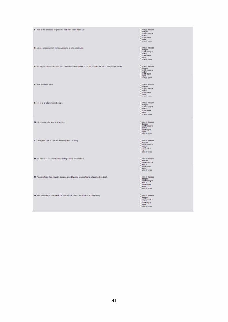
41