seventh framework programme research … · · 2017-04-22software tool: microsoft word 2007...
TRANSCRIPT

SEVENTH FRAMEWORK PROGRAMME Research Infrastructures
INFRA-2011-2.3.5 – Second Implementation Phase of the European High Performance Computing (HPC) service PRACE
PRACE-2IP
PRACE Second Implementation Project
Grant Agreement Number: RI-283493
D8.1.4
Plan for Community Code Refactoring Final
Version: 1.0 Author(s): Claudio Gheller, Will Sawyer (CSCS) Date: 24.02.2012

D8.1.4 Plan for Community Code Refactoring
PRACE-2IP - RI-283493 24.02.20122 i
Project and Deliverable Information Sheet
PRACE Project Project Ref. №: RI-283493 Project Title: PRACE Second Implementation Project Project Web Site: http://www.prace-project.eu Deliverable ID: D8.1.4 Deliverable Nature: Report Deliverable Level: PU *
Contractual Date of Delivery: 29 / 02 / 2012 Actual Date of Delivery: 29 / 02 / 2012
EC Project Officer: Thomas Reibe * - The dissemination level are indicated as follows: PU – Public, PP – Restricted to other participants (including the Commission Services), RE – Restricted to a group specified by the consortium (including the Commission Services). CO – Confidential, only for members of the consortium (including the Commission Services).
Document Control Sheet
Document
Title: Plan for Community Code RefactoringID: D8.1.4 Version: 1.0
Status: Final
Available at: http://www.prace-project.eu Software Tool: Microsoft Word 2007 File(s): D8.1.4.docx
Authorship
Written by: Claudio Gheller, Will Sawyer (CSCS) Contributors: Thomas Schulthess, CSCS; Fabio Affinito,
CINECA; Ivan Girotto, Alastair McKinstry, Filippo Spiga, ICHEC; Laurent Crouzet, CEA; Andy Sunderland, STFC; Giannis Koutsou, Abdou Abdel-Rehim, CASTORC; Fernando Nogueira, Miguel Avillez , UC-LCA; Georg Huhs, José María Cela, and Mohammad Jowkar, BSC, Nikos Anastopoulos (ICCS-GRNET), Paulo Silva (UC)
Reviewed by: Michael Schliephake, KTH Thomas Eickermann, JUELICH
Approved by: MB/EB

D8.1.4 Plan for Community Code Refactoring
PRACE-2IP - RI-283493 24.02.20122 ii
Document Status Sheet
Version Date Status Comments 0.1 02/01/2012 First skeleton 0.2 10/01/2012 Overall structure defined 0.3 21/01/2012 First performance model added 0.4 23/01/2012 More performance models 0.5 26/01/2012 More performance models 0.6 01/02/2012 Appendix B added 0.7 03/02/2012 More performance models 0.8 07/02/2012 More performance models and
conclusions added
0.9 08/02/2012 Proofreading 1.0 09/02/2012 Final version

D8.1.4 Plan for Community Code Refactoring
PRACE-2IP - RI-283493 24.02.20122 iii
Document Keywords
Keywords: PRACE, HPC, Research Infrastructure, scientific applications,
libraries, performance modelling.
Disclaimer This deliverable has been prepared by Work Package 8 of the Project in accordance with the Consortium Agreement and the Grant Agreement n° RI-283493. It solely reflects the opinion of the parties to such agreements on a collective basis in the context of the Project and to the extent foreseen in such agreements. Please note that even though all participants to the Project are members of PRACE AISBL, this deliverable has not been approved by the Council of PRACE AISBL and therefore does not emanate from it nor should it be considered to reflect PRACE AISBL’s individual opinion.
Copyright notices 2011 PRACE Consortium Partners. All rights reserved. This document is a project document of the PRACE project. All contents are reserved by default and may not be disclosed to third parties without the written consent of the PRACE partners, except as mandated by the European Commission contract RI-283493 for reviewing and dissemination purposes.
All trademarks and other rights on third party products mentioned in this document are acknowledged as own by the respective holders.

D8.1.4 Plan for Community Code Refactoring
PRACE-2IP - RI-283493 24.02.20122 iv
Table of Contents
Project and Deliverable Information Sheet .......................................................................... i
Document Control Sheet ...................................................................................................... i
Document Status Sheet ...................................................................................................... ii
Document Keywords .......................................................................................................... iii
Table of Contents ................................................................................................................ iv
List of Figures ...................................................................................................................... vi
References and Applicable Documents ............................................................................. viii
List of Acronyms and Abbreviations ..................................................................................... x
Executive Summary ............................................................................................................ 1
1 Introduction ..................................................................................................................... 1
2 Astrophysics ..................................................................................................................... 4 2.1 RAMSES ................................................................................................................................. 4 2.2 PKDGRAV ............................................................................................................................ 10 2.3 PFARM ................................................................................................................................ 12 Implementation ........................................................................................................................ 16 Testing and Optimization .......................................................................................................... 16
3 Climate .......................................................................................................................... 18 3.1 Couplers: OASIS ................................................................................................................... 18 3.2 Input/Output: CDI, XIOS, PIO ............................................................................................... 19 3.3 Dynamical Cores: ICON ........................................................................................................ 20 3.4 Ocean Models: NEMO and Fluidity‐ICOM ............................................................................ 24
4 Material Science ............................................................................................................ 39 4.1 ABINIT ................................................................................................................................. 39 4.2 Quantum ESPRESSO ............................................................................................................ 55 4.3 Yambo ................................................................................................................................. 59 4.4 Siesta .................................................................................................................................. 59 4.5 Octopus ............................................................................................................................... 62 4.6 Exciting/ELK ......................................................................................................................... 63
5 Particle Physics .............................................................................................................. 67 5.1 Target codes, algorithms, and architectures ........................................................................ 67 5.2 Workplan ............................................................................................................................ 71
6 Conclusions and next steps ............................................................................................ 74
Appendix A. Engineering Community ................................................................................ 75 A.1 Scientific Challenges ............................................................................................................ 75 A.2 Method to approach the Community .................................................................................. 77 A.3 Numerical Approaches and Community Codes .................................................................... 80 A.4 Community involvement, expected outcomes and their impact .......................................... 89 A.5 Relevant Bibliography ......................................................................................................... 90
Appendix B. Description of the linear‐response methodology of ABINIT, and performance analysis. ............................................................................................................................ 93
B.1 Motivation .......................................................................................................................... 93 B.2 Performances of the linear‐response part of ABINIT ............................................................ 93

D8.1.4 Plan for Community Code Refactoring
PRACE-2IP - RI-283493 24.02.20122 v
B.3 Performance improvement of the linear‐response part of ABINIT. ...................................... 97

D8.1.4 Plan for Community Code Refactoring
PRACE-2IP - RI-283493 24.02.20122 vi
List of Figures
Figure 1: GANTT for RAMSES refactoring ......................................................................................... 10 Figure 2: Distribution of absolute time spent in different parts of the code td different timestep levels in runs with 1000 (left) and 2000 (right) processors. The solid lines show the time for the various sections integrated on the various time levels. ...................................................................................... 11 Figure 3: GANTT for PKDGRAV refactoring. .................................................................................... 12 Figure 4: Example Process Decomposition in the EXAS Stage ........................................................... 13 Figure 5: GANTT chart for PFARM. .................................................................................................... 16 Figure 6: OASIS3-MCT: Coupling exchange ....................................................................................... 18 Figure 7: time spent in OASIS3-MCT initialisation ............................................................................. 19 Figure 8: GANTT chart for OASIS ....................................................................................................... 19 Figure 9: The Roofline Model provides a simple mechanism for predicting application performance based on two benchmarks. The performance figures given are for a quad-core Opteron 8380 (2.5 GHz). ..................................................................................................................................................... 21 Figure 10 : The roughly 60 ICON NH kernels vary in computational intensity and performance. The outlying kernels on the right and left are part of the vertical implicit solver, which has loop dependencies and has to run sequentially, noticeably reducing performance. ...................................... 21 Figure 11: Predicted and measured single-node ICON-NH execution times for R2B3 and R2B4 resolution (1000 iterations) ................................................................................................................... 22 Figure 12: The aggregated time for computation (blue) and communication (red), for R2B4 and R2B5 on a Cray XK6 with 16 cores per node. Optimal scaling would yield horizontal lines. Green (AMD Interlagos), purple (Intel Westmere) and light blue (NVIDIA M2090) indicate the predicted times for those architectures assuming optimal scaling, and these timings are therefore a worst-case scenario for communication. ..................................................................................................................................... 23 Figure 13: Timeline for ICON dynamical core efforts .......................................................................... 24 Figure 14: Time spent in compute and data transport in the tra_adv_tvd kernel for the ORCA1 grid when running on a single Nehalem (Westmere) core and a Tesla (Fermi) GPU. The 2nd bar shows performance before halo transfers were optimised. .............................................................................. 29 Figure 15: Speed-up of the OpenMP version of tra_ldf_iso w.r.t. its performance on an NVIDIA Tesla GPU. In each case the no. of cores utilized is the same as the no. of OpenMP threads. Results are the averages of three runs for the ORCA2_LIM case. ................................................................................ 30 Figure 16: Scaling performance of the OpenMP version of the lim_rhg kernel on a Nehalem compute node for the ORCA2 and ORCA025 datasets. ...................................................................................... 31 Figure 17: Profile of the OpenMP version of the lim_rhg kernel as the number of OpenMP threads is increased. Results are for the ORCA2 dataset run on HECToR IIb. ..................................................... 31 Figure 18: GANTT chart for Fault Tolerant NEMO ............................................................................. 33 Figure 19: Speedup comparison between matrix local assembly and nonlocal assembly .................... 35 Figure 20: Comparison between using critical directive and without critical directive ........................ 36 Figure 21: Performance comparison between pure MPI version and pure OpenMP versions .............. 37 Figure 22: CPU time (sec.) per process needed by a single call to ZHEEV ScaLAPACK routine with respect to number of MPI process for several sizes of square matrix (512, 1024, 2048) and several ScaLAPACK implementations ............................................................................................................... 40 Figure 23: CPU time distribution for the ABINIT parallel eigensolver (standard test case: 107 gold atoms) with respect to the number of “band” cores (npband) and “FFT” cores (npfft). ....................... 42 Figure 24: Repartition of CPU time in ABINIT routines varying the number of CPU cores. .............. 42 Figure 25: BigDFT on Titane-CCRT supercomputer: efficiency (solid blue curve) and speedup (dashed red line) with respect to the number of MPI processes and threads. ....................................... 44 Figure 26: BigDFT on Palu-CSCS supercomputer: efficiency (solid blue curve) and speedup (dashed red line) with respect to the number of MPI processes and threads. ..................................................... 45 Figure 27: Computer of time spent in convolutions on two different architectures (Titane-CCRT and Palu-CSCS) ........................................................................................................................................... 45 Figure 28: Speedup of BigDFT using GPUs ......................................................................................... 46 Figure 29: Parallel efficiency of new FFTW implementation in ABINIT-GW using multithreaded FFTW3 library ....................................................................................................................................... 48

D8.1.4 Plan for Community Code Refactoring
PRACE-2IP - RI-283493 24.02.20122 vii
Figure 30: Parallel efficiency polarisability and self-energy kernels in ABINIT-GW using openMP . 49 Figure 31: Performance of the new implementation of the inversion of the dieletric matrix using ScaLAPACK .......................................................................................................................................... 49 Figure 32: GANTT chart for Yambo .................................................................................................... 59 Figure 33: Visualisation of the outer two levels of parallelisation. The first level is the division of the domain. The first step in each domain is solving the linear systems, which can be done in parallel. Afterwards all processors can be used for doing the following computations in parallel. .................... 61 Figure 34: GANTT chart for the work on SS algorithm. ...................................................................... 61 Figure 35: GANTT chart for Octopus. .................................................................................................. 63 Figure 36: GANTT chart for Exciting/ELK .......................................................................................... 66 Figure 37: A schematic presentation of the Lattice setup in 2 dimensions ........................................... 67 Figure 38: Profiling of the twisted mass CG solver code on 24 nodes. Center for User and MPI functions with respect to the total time. The right chart is a break-down of the User functions (percentages are with respect to the total time spent in User functions) and the left chart is a break-down of the MPI functions (percentages are with respect to the total time spent in MPI functions). Run was performed on Cray XE6 at NERSC for a lattice with 48 sites in the spatial directions and 96 sites on the time direction. ............................................................................................................................. 68 Figure 39: Strong scaling test of the twisted mass CG solver on a CrayXE6. The points labeled “Time restricted to node” refer to scaling tests carried out where care was taken so that the spatial lattice sites where mapped to the physical 3D torus topology of the machine’s network, which restricts the time-dimension partitioning to a node. .......................................................................................................... 69 Figure 40: measuring the effective memory bandwidth for single core on a Cray XE6 as a function of the buffer size. ....................................................................................................................................... 70 Figure 41: Rooflines (coloured) for attainable floating point performance for a node of the Cray XE6 machine at NERSC. Each node has 4 sockets with 6 cores each. Both vendor and measured data are shown .................................................................................................................................................... 71 Figure 42: World marketed energy consumption, 1990-2035 (source: International Energy Outlook 2010)...................................................................................................................................................... 76 Figure 43: Increase of number of cores in fastest European HPC systems ........................................... 76 Figure 44: (Code Alya): Free surface for flushing toilet (left), external aerodynamic, LES model (right) ..................................................................................................................................................... 83 Figure 45: (Code APES) Flow through a spacer geometry of an electrodialysis device (left), a foam used as a silencer, meshed with seeder (right) ...................................................................................... 83 Figure 46: (Code Elmer) Cavity lid case solved with the monolithic Navier-Stokes solver (GMRES with IL0 preconditioner) ....................................................................................................................... 84 Figure 47: (Code_Aster) SALOME-MECA: results display (left), Calculation of a combustion turbine compressor: bladed rotor and quarter compressor (right) ..................................................................... 85 Figure 48: (Code_Saturne) Flow in bundle of tubes (left), Air quality study of an operating theatre (right) ..................................................................................................................................................... 86 Figure 49: (Code N3D) Illustration of laminar-turbulent transition in a flat-plate boundary layer (left), application of DNS to control laminar- turbulent transition on the wing of an airliner (right) ............. 87 Figure 50: (Code TELEMAC) Salinity distribution in the Berre Lagoon (TELEMAC3D) (left), Flow evolution after the Malpasset dam broke (TELEMAC2D) (right) ........................................................ 88 Figure 51: (Code ZFS) Generated fully automatically lung: Mesh for the first 6 bifurcations of a human lung (left), Mesh for an internal combustion engine (right) ...................................................... 89 Figure 52: Speedup of the most costly code sections that show good scaling. ..................................... 96 Figure 53: Relative amount of wall clock time for the most costly code sections. ............................... 97

D8.1.4 Plan for Community Code Refactoring
PRACE-2IP - RI-283493 24.02.20122 viii
References and Applicable Documents
[1] http://www.prace-ri.eu/PRACE-Second-Implementation-Phase [2] Deliverable D8.1.1: “Community Codes Development Proposal” [3] Deliverable D8.1.2: “Performance Model of Community Codes” [4] Deliverable D8.1.3: “Prototype Codes Exploring Performance Improvements” [5] Bridging Performance Analysis Tools and Analytic Performance Modeling for HPC, T. Hoefler, Proceedings of Workshop on Productivity and Performance (PROPER 2010), Springer, Dec. 2010. [6] A Framework for Performance Modeling and Prediction. Allan Snavely , Laura Carrington , Nicole Wolter , Jesus Labarta, Rosa Badia , Avi Purkayastha, Proceedings of the 2002 ACM/IEEE conference on Supercomputing. [7] Performance Modeling: Understanding the Present and Predicting the Future. Bailey, David H.; Snavely, Allan. http://escholarship.org/uc/item/1jp3949m [8] How Well Can Simple Metrics Represent the Performance of HPC Applications? Laura C. Carrington, Michael Laurenzano, Allan Snavely, Roy L. Campbell, Larry P. Davis; Proceedings of the 2005 ACM/IEEE conference on Supercomputing, 2005, IEEE Computer Society [9] http://web.me.com/romain.teyssier/Site/RAMSES.html [10] https://hpcforge.org/projects/pkdgrav2/ [11] J. Barnes and P. Hut (December 1986). "A hierarchical O(N log N) force-calculation algorithm". Nature 324 (4): 446-44 [12] http://lca.ucsd.edu/portal/software/enzoFLASH [13] ICON testbed; https://code.zmaw.de/projects/icontestbed [14] ICOMEX project; http://wr.informatik.uni-hamburg.de/research/projects/icomex [15] Williams, S.; A. Waterman, and D. Patterson, "Roofline: An Insightful Visual Performance Model for Floating-Point Programs and Multicore Architectures", Communications of the ACM (CACM), April 2009. [16] Conti, C; W. Sawyer: GPU Accelerated Computation of the ICON Model. CSCS Internal Report, 2011. A G Sunderland, C J Noble, V M Burke and P G Burke, CPC 145 (2002), 311-340. [17] A G Sunderland, C J Noble, V M Burke and P G Burke, CPC 145 (2002), 311-340. [18] Future Proof Parallelism for Electron-Atom Scattering Codes with PRMAT, A. Sunderland, C. Noble, M. Plummer, http://www.hector.ac.uk/cse/distributedcse/reports/prmat/. [19] The Parallel Linear Algebra for Multicore Architectures project, http://icl.cs.utk.edu/plasma/. [20] The Matrix Algebra on GPU and Multicore Architectures project, http://icl.cs.utk.edu/magma/. [21] Single Node Performance Analysis of Applications on HPCx, M. Bull, HPCx Technical Report HPCxTR0703 (2007). [22] Combined-Multicore Parallelism for the UK electron-atom scattering Inner Region R-matrix codes on HECToR, HECToR Distributed CSE Support projects, http://www.hector.ac.uk/cse/distributedcse/projects/. [23] Wolfe, M. and C. Toepfer, ‘The PGI Accelerator Programming Model on NVIDIA GPUs Part 3: Porting WRF’, PGI Insider Article, October 2009, (http://www.pgroup.com/lit/articles/insider/v1n3a1.htm). [24] Pain, C.C.; M.D. Piggot, A.J.H. Goddard, F. Fang, G.J. Gorman, D.P. Marshall, M.D. Eaton, P.W. Power, and C.R.E. de Oliveira: Three-dimensional unstructured mesh ocean modelling. Ocean Modelling, 10(1-2), 5-33, 2005. [25] http://www.hector.ac.uk [26] http:// www.top500.org

D8.1.4 Plan for Community Code Refactoring
PRACE-2IP - RI-283493 24.02.20122 ix
[27] Ewald P. (1921) "Die Berechnung optischer und elektrostatischer Gitterpotentiale", Ann. Phys. 369, 253–287. [28] Long Wang et al., Large Scale Plane Wave Pseudopotential Density Functional Theory Calculations on GPU Clusters, SC2011 [29] Spiga F. & Girotto I., phiGEMM: a CPU-GPU library for porting Quantum ESPRESSO on hybrid systems, 20th Euromicro International Conference on Parallel, Distributed and Network-Based Computing (PDP2012), Special Session on GPU Computing and Hybrid Computing, February 15-17, 2012, Garching (Germany) - accepted [30] http://www.tddft.org [31] Craig, A.; M. Vertenstein and R. Jacob: “A new flexible coupler for earth system modeling developed for CCSM4 and CESM1”, Int. J. High Perf. Comput. Appl.. In press. [32] http://www.tddft.org/programs/octopus/wiki/index.php/Main_Page [33] http://www.yambo-code.org/ [34] http://www.abinit.org/ [35] http://www.quantum-espresso.org/ [36] http://www.icmab.es/dmmis/leem/siesta/ [37] A. M, Khokhlov, Fully Threaded Tree Algorithms for Adaptive Refinement Fluid Dynamics Simulations, 1998, Journal of Computational Physics, 143, 519 [38] http://lca.ucsd.edu/portal/software/enzo [39] http://www.mpa-garching.mpg.de/gadget/ [40] http://code.google.com/p/cusp-library/ [41] A G Sunderland, C J Noble, V M Burke and P G Burke, CPC 145 (2002), 311-340. [42] K L Baluja, P G Burke and L A Morgan, CPC 27 (1982), 299-307. [43] Single Node Performance Analysis of Applications on HPCx, M. Bull, HPCx Technical Report HPCxTR0703 (2007) http://www.hpcx.ac.uk/research/hpc/technical_reports/HPCxTR0703.pdf. [44] Eigenvalue Solvers for Petaflop-Applications, http://elpa.rzg.mpg.de [45] Matrix Algebra on GPU and Multicore Architectures, http://icl.cs.utk.edu/magma/ [46] Future Proof Parallelism for Electron-Atom Scattering Codes with PRMAT, A. Sunderland, C. Noble, M. Plummer, http://www.hector.ac.uk/cse/distributedcse/reports/prmat/. [47] V M Burke and C J Noble, CPC 85 (1995), 471-500; V M Burke, C J Noble, V Faro-Maza, A Maniopoulou and N S Scott, CPC 180 (2009), 2450-2451 [48] M H Alexander, J Chem Phys 81 (1984) 4510-4516; M H Alexander and D E Manolopoulos, J Chem Phys 86 (1987) 2044-2050. [49] http://amcg.ese.ic.ac.uk/index.php?title=Modelling_Software [50] http://code.google.com/p/gperftools/?redir=1 [51] http://buildbot.sourceforge.net/ [52] Madec, G: NEMO ocean engine, Note du Pole de modélisation, Institut Pierre-Simon Laplace (IPSL), France, No 27 ISSN No 1288-1619, 2008. [53] Skamarock, W. C., J. B. Klemp, J. Dudhia, D. O. Gill, D. M. Barker, W. Wang, and J. G. Powers, 2005: A description of the Advanced Research WRF Version 2. NCAR Tech Notes-468+STR [54] Alexander F. Shchepetkin, James C. McWilliams, “The regional oceanic modeling system (ROMS): a split-explicit, free-surface, topography-following-coordinate oceanic model ”, Ocean Modelling, Vol. 9, No. 4. (2005), pp. 347-40. [55] A. R. Porter and M. Ashworth, “Optimising and Configuring the Weather Research and Forecast Model on the Cray XT,” Cray User Group Meeting, Edinburgh, 2010. [56] OP2 Project Page: http://people.maths.ox.ac.uk/gilesm/op2/ [57] K. Jansen and C. Urbach‚ ‘‘tmLQCD: A rogram suite to simulate Wilson Twisted mass Lattice QCD``, Comput. Phys. Coomun. 180:2717-2738, 2009 [arXiv:0905.3331].

D8.1.4 Plan for Community Code Refactoring
PRACE-2IP - RI-283493 24.02.20122 x
[58] M. A. Clark, et.al. ``Solving Lattice QCD systems of equations using mixed precision solvers on GPUs``, Comput. Phys. Commun. 181:1517-1528,2010 [arXiv:0911.3191]. [59] http://en.wikipedia.org/wiki/Advanced_Vector_Extensions.
List of Acronyms and Abbreviations
AMCG Applied Modelling and Computation Group AMG Algebraic MultiGrid AMR Adaptive Mesh Refinement API Application Programming Interface AVX Advanced Vector Extensions BCSR Blocked Compressed Sparse-Row BICGSTAB BIConjugate Gradient STABilized method BLAS Basic Linear Algebra Subprograms BSC Barcelona Supercomputing Center (Spain) BTU British thermal unit CAD Computer Aided Design CAF Co-Array Fortran CCLM COSMO Climate Limited-area Model ccNUMA cache coherent NUMA CDI Climate Data Interface, from MPI-M CEA Commissariat à l’Energie Atomique (represented in PRACE by GENCI,
France) CERFACS The European Centre for Research and Advanced Training in Scientific
Computation CESM Community Earth System Model, developed at NCAR (USA) CFD Computational Fluid Dynamics CG Conjugate-Gradient CINECA Consorzio Interuniversitario, the largest Italian computing centre (Italy) CINES Centre Informatique National de l’Enseignement Supérieur (represented
in PRACE by GENCI, France) CM Computational Mechanics CMCC Centro Euro-Mediterraneo per i Cambiamenti Climatici CNRS Centre national de la recherche scientifique COSMO Consortium for Small-scale Modeling CP Car-Parrinello CPU Central Processing Unit CSC Finnish IT Centre for Science (Finland) CSCS The Swiss National Supercomputing Centre (represented in PRACE by
ETHZ, Switzerland) CSD Computational Solid Dynamics CSR Compressed Sparse Row format CUBLAS CUda BLAS CUDA Compute Unified Device Architecture (NVIDIA) CUSP CUda SParse linear algebra library DECI Distributed European Computing Initiative DEISA Distributed European Infrastructure for Supercomputing Applications.
EU project by leading national HPC centres.

D8.1.4 Plan for Community Code Refactoring
PRACE-2IP - RI-283493 24.02.20122 xi
DFPT Density-Functional Perturbation Theory DFT Density Functional Theory (also Discrete Fourier Transform) DGEMM Double precision General Matrix Multiply DKRZ Deutsches Klimarechenzentum DP Double Precision, usually 64-bit floating-point numbers DRAM Dynamic Random Access memory DSL Domain-specific Language EC European Community EDF Electricite de France ELPA Eigenvalue SoLvers for Petaflop-Applications ENES European Network for Earth System Modelling EPCC Edinburgh Parallel Computing Centre (represented in PRACE by
EPSRC, United Kingdom) EPSRC The Engineering and Physical Sciences Research Council (United
Kingdom) ESM Earth System Model ETHZ Eidgenössische Technische Hochschule Zürich, ETH Zurich
(Switzerland) ETMC European Twisted Mass Collaboration ETSF European Theoretical Spectroscopy Facility ESFRI European Strategy Forum on Research Infrastructures; created
roadmap for pan-European Research Infrastructure. FE Finite Elements FETI Finite Element Tearing and Interconnecting FFT Fast Fourier Transform FP Floating-Point FPGA Field Programmable Gate Array FPU Floating-Point Unit FV Finite Volumes FT-MPI Fault Tolerant Message Passing Interface FZJ Forschungszentrum Jülich (Germany) GB Giga (= 230 ~ 109) Bytes (= 8 bits), also GByte Gb/s Giga (= 109) bits per second, also Gbit/s GB/s Giga (= 109) Bytes (= 8 bits) per second, also GByte/s GCS Gauss Centre for Supercomputing (Germany) GENCI Grand Equipement National de Calcul Intensif (France) GFlop/s Giga (= 109) Floating-point operations (usually in 64-bit, i.e., DP) per
second, also GF/s GGA Generalised Gradient Approximations GHz Giga (= 109) Hertz, frequency =109 periods or clock cycles per second GMG Geometric MultiGrid GMRES Generalized Minimal RESidual method GNU GNU’s not Unix, a free OS GPGPU General Purpose GPU GPL GNU General Public Licence GPU Graphic Processing Unit GRIB GRIdded Binary HDD Hard Disk Drive HECToR High End Computing Terascale Resources HMPP Hybrid Multi-core Parallel Programming (CAPS enterprise)

D8.1.4 Plan for Community Code Refactoring
PRACE-2IP - RI-283493 24.02.20122 xii
HPC High Performance Computing; Computing at a high performance level at any given time; often used synonym with Supercomputing
HPL High Performance LINPACK ICHEC Irish Centre for High-End Computing ICOM Imperial College Ocean Model ICON Icosahedral Non-hydrostatic model IDRIS Institut du Développement et des Ressources en Informatique
Scientifique (represented in PRACE by GENCI, France) IEEE Institute of Electrical and Electronic Engineers IESP International Exascale Project I/O Input/Output IPSL Institut Pierre Simon Laplace IS-ENES Infrastructure for the European Network for Earth System Modelling JSC Jülich Supercomputing Centre (FZJ, Germany) KB Kilo (= 210 ~103) Bytes (= 8 bits), also KByte LAPACK Linear Algebra PACKage LB Lattice Boltzmann LBE Lattice Boltzmann Equation LES Large-Eddy Simulation LINPACK Software library for Linear Algebra LQCD Lattice QCD LRZ Leibniz Supercomputing Centre (Garching, Germany) MAGMA Matrix Algebra on GPU and Multicore Architectures MB Mega (= 220 ~ 106) Bytes (= 8 bits), also MByte MB/s Mega (= 106) Bytes (= 8 bits) per second, also MByte/s MBPT Many-Body Perturbation Theory MCT Model Coupling Toolkit, developed at Argonne National Lab. (USA) MD Molecular Dynamics MFlop/s Mega (= 106) Floating-point operations (usually in 64-bit, i.e., DP) per
second, also MF/s MHz Mega (= 106) Hertz, frequency =106 periods or clock cycles per second MIC Many Integrated Core MIPS Originally Microprocessor without Interlocked Pipeline Stages; a RISC
processor architecture developed by MIPS Technology MKL Math Kernel Library (Intel) MPI Message Passing Interface MPI-IO Message Passing Interface – Input/Output MPI-M MPI for Mathematics MPP Massively Parallel Processing (or Processor) MPT Message Passing Toolkit NCAR National Center for Atmospheric Research NCF Netherlands Computing Facilities (Netherlands) NEGF non-equilibrium Green's functions, NERC Natural Environment Research Council NEMO Nucleus for European Modeling of the Ocean NERC Natural Environment Research Council (United Kingdom) NetCDF Network Common Data Form NUMA Non Uniform Memory Access NWP Numerical Weather Prediction OpenCL Open Computing Language OECD Organisation for Economic Co-operation and Development

D8.1.4 Plan for Community Code Refactoring
PRACE-2IP - RI-283493 24.02.20122 xiii
OpenMP Open Multi-Processing OS Operating System PAW Projector Augmented-Wave PETSc Portable, Extensible Toolkit for Scientific computation PGI Portland Group, Inc. PGAS Partitioned Global Address Space PIMD Path-Integral Molecular Dynamics PIO Parallel I/O PLASMA Parallel Linear Algebra for Scalable Multi-core Architectures POSIX Portable OS Interface for Unix PPE PowerPC Processor Element (in a Cell processor) PRACE Partnership for Advanced Computing in Europe; Project Acronym PSNC Poznan Supercomputing and Networking Centre (Poland) PWscf Plane-Wave Self-Consistent Field QCD Quantum Chromodynamics QR QR method or algorithm: a procedure in linear algebra to factorise a
matrix into a product of an orthogonal and an upper triangular matrix RAM Random Access Memory RDMA Remote Data Memory Access RISC Reduce Instruction Set Computer RPM Revolution per Minute RWTH Rheinisch-Westfaelische Technische Hochschule Aachen ScaLAPACK Scalable LAPACK ScalES Scalable Earth System model SGEMM Single precision General Matrix Multiply, subroutine in the BLAS SHMEM Share Memory access library (Cray) SIMD Single Instruction Multiple Data SM Streaming Multiprocessor, also Subnet Manager SMP Symmetric MultiProcessing SP Single Precision, usually 32-bit floating-point numbers SPH Smoothed Particle Hydrodynamics STFC Science and Technology Facilities Council (represented in PRACE by
EPSRC, United Kingdom) STRATOS PRACE advisory group for STRAtegic TechnOlogieS TB Tera (=240 ~ 1012) Bytes (= 8 bits), also TByte TDDFT Time-dependent density functional theory TFlop/s Tera (=1012) Floating-point operations (usually in 64-bit, i.e., DP) per
second, also TF/s Tier-0 Denotes the apex of a conceptual pyramid of HPC systems. In this
context the Supercomputing Research Infrastructure would host the Tier-0 systems; national or topical HPC centres would constitute Tier-1
UMFPACK Unsymmetric Multifrontal sparse LU Factorization package UML Unified Modeling Language UPC Unified Parallel C WRF Weather Research & Forecasting XIOS XML IO Server, from IPSL

D8.1.4 Plan for Community Code Refactoring
PRACE-2IP - RI-283493 24.02.20122
1
Executive Summary
In this deliverable we present the scientific codes performance modelling carried out during the first six months of work package 8 of PRACE-2IP. For each code selected in the domains of Astrophysics, Material Science, Climate and Particle Physics, we provide a short summary of the algorithms to be the subject of refactoring. A detailed description of the proposed work and its motivations are reported, for most cases motivated through a performance modelling analysis. Each code is supplied with a standard test suite, which allows the verification of quality and correctness of the re-implemented software. A detailed workplan for the implementation phase (M7-20) is presented for each application, specifying the timeline and the milestones for its refactoring, and clearly stating the main objectives of the development work.
In the deliverable we also introduce a fifth scientific community, Engineering, which has recently joined the work package. At the time of the submission of the current document, this community has identified the relevant applications and specified the main targets for code refactoring. The performance analysis and modelling will be added as soon as data and results are available.
1 Introduction In the first four months, PRACE-2IP [1] work package 8 (hereafter WP8) selected a number of scientific communities that expressed a specific interest in having their numerical codes enabled to the coming generation of HPC systems, and which were willing to contribute to their development and refactoring. They recognised the value of exploiting new powerful architectures and at the same time they realized the peculiarities of these new architectures that, in order to be properly and effectively used, require redesign of codes in a close and synergic interaction between community code developers and HPC experts.
Communities’ representatives proposed a list of relevant numerical applications that have been the subject of a first screening procedure, in order to identify those most promising (from the HPC point of view). The selected codes were then analysed in terms of algorithms, of adopted parallel strategies and paradigms and of actual performances (estimated on available computing platforms) in order to verify their suitability to the envisaged refactoring work. The list of these codes is presented in Table 1.
These steps have been extensively described in deliverables D8.1.1 [2], D8.1.2 [3] and D8.1.3 [4]. Note that a few codes in the list presented here were not present in D8.1.3. In particular the ELK/EXCITING performance analysis could not be completed and presented on time in the previous deliverable. The missing information and the performance model are added here. Furthermore, one more Material Science module has been added to the ABINIT package, and its performance analysis is described Appendix B.
All the collected information and data are now used to complete the performance model of the different codes. A performance model allows one to express the performances of a code analytically as a function of its main algorithmic features and of the hardware architectural characteristics. The performance modelling methodology [5][6][7][8] was introduced in D8.1.2. It is used to identify the numerical kernels on which the redesign and refactoring work must specifically focus, and to predict performances on new HPC systems.
The results of the performance modelling of the selected code are presented in this document. Note that not all the resulting models have the same degree of sophistication, depending on the complexity of the code and the algorithms, the experience and knowledge of the

D8.1.4 Plan for Community Code Refactoring
PRACE-2IP - RI-283493 24.02.20122
2
community developers and last, but not least, the level of detail needed to identify the targets for refactoring. In all cases, we present a detailed description of the expected work, with accurate justifications of the proposed choices and a clear plan for code design and refactoring
For each code, we also present the testing and validation procedure that will be adopted to verify that the software produced by WP8 works properly and produces results compatible with those generated by the original codes.
Finally, we also describe the specific refactoring workplan for each of the selected applications, setting timelines and milestones, toward the M20 software release, which will be followed by the acceptance procedure, based on the presented tests.
Domain Application Usage Astrophysics RAMSES Galaxy - cluster of galaxy evolution
PKDGRAV Large scale structure of the universe, precision cosmology
PFARM Electron-atom scattering Climate OASIS Full climate modelling, coupler
CDI/XIOS/PIO Efficient I/O libraries ICON Dynamical core NEMO/ICOM Ocean models
Material Science ABINIT Density functional theory, Density-Functional perturbation theory, Many-Body perturbation theory, Time-Dependent Density functional theory
Quantum ESPRESSO
Density‐Functional theory, Plane Waves, and Pseudo-Potentials, Projector‐Augmented waves
YAMBO Many-Body perturbation theory, Time-Dependent Density functional theory
SIESTA Electronic structure calculations and ab-initio molecular dynamics
OCTOPUS Density Functional Theory Exciting/ELK Full-Potential Linearized Augmented-Plane
Wave Particle Physics tmQCD Lattice QCD
Table 1: Codes selected for performance modelling.
In the current deliverable, we also introduce Engineering as a further scientific domain whose applications will be subject of redesign and refactoring. This late addition was possible due to the scientific community procedure introduced in D8.1.1 and justified by the large interest expressed by additional communities to have their codes exploiting novel HPC architectures. Due to the late start-up, at the time of the submission of the current document, this community has identified the relevant applications and specified the main targets for code refactoring. The performance analysis and modelling are on-going and will be formally reported (as addendum to the current or annex to a future deliverable) as soon as data and results are available.
This document is organized as follows. Sections 2 to 6 are dedicated each to a different scientific domain: Astrophysics (Section 2), Climate (Section 3), Material Science (Section 4) and Particle Physics (Section 5). All sections report a short overview, the performance modelling results and the testing and validation procedure for each of the codes under

D8.1.4 Plan for Community Code Refactoring
PRACE-2IP - RI-283493 24.02.20122
3
investigation in the corresponding community. The specific work plans for each code are presented as well. The Engineering community, the related selection procedure and the codes description is reported in Appendix A, that follows the Conclusions Section (Section 6). Finally, Appendix B presents the linear-response methodology, the new ABINIT module and its performance analysis.

D8.1.4 Plan for Community Code Refactoring
PRACE-2IP - RI-283493 24.02.20122
4
2 Astrophysics In this section we give a short overview of the three codes selected for Astrophysics, and we complete their performance modelling by presenting the projected performance for novel HPC architectures. The three codes have been already extensively analysed in the previous deliverables D8.1.2 [3] and D8.1.3 [4]. For each code we describe the testing and validation procedure that will be adopted to verify the correctness of the accomplished refactoring work. Finally, we describe the work plan for the re-design and implementation of the various algorithms.
2.1 RAMSES
2.1.1 Overview
The RAMSES code [9] is an adaptive mesh refinement (AMR) multi-species code, describing the behaviour of both the baryonic component, represented as a fluid on the cells of the AMR mesh, and the dark matter, represented as a set of collisionless particles. The two matter components interact via gravitational forces. The AMR approach makes it possible to get high spatial resolution only where this is actually required, thus ensuring a minimal memory usage and computational effort.
During the performance analysis phase [3], we identified the most computational demanding parts of the RAMSES code as the Hydro and the Gravity kernels together with the related communication infrastructure.
For the Hydro kernel the performance is strongly dependent from the AMR data structure. In fact, memory contiguity of two neighbouring Octs, the fundamental cells of the adaptive computational mesh, is not enforced. Therefore the corresponding data can be far from each other in the memory of the same processor or even in the memory of two different processors. Furthermore, despite the usage of the space filling curves, the load is not perfectly balanced between processors. This problem grows with the number of processors, since smaller chunks of data are assigned to each of them. This means that first the data distribution tends to be more and more heterogeneous, leading to higher imbalances of the work. Second, in order to build the AuxBoxes (small data cubes used for solving hydrodynamics equations), each processor has to access information stored on a larger number of processors, affecting strongly the network load and the communication overhead. All the details and the formal definition of the Oct and the AuxBox data structures can be found in [4]. In order to improve the performances, both the load balancing must be improved and the communication overhead must be reduced. This can be obtained either working on the basic algorithmic architecture, changing the AMR data structure, or on the domain decomposition strategy, increasing data locality. These solutions, however, are extremely invasive, from an algorithmic point of view, leading to deep changes in the software architecture. A third feasible solution is that of exploiting some specific hardware solutions, like multi-core nodes with large shared memory and accelerators.
In order to exploit shared memory, the Hydro kernel has to be re-implemented with a hybrid OpenMP+MPI approach. This, in principle, could be accomplished by an OpenMP parallel loop running on all the active cells stored in each node. However, specific care must be devoted in managing the access to the shared memory.
Accelerators, like GPUs or MIC, can strongly improve the performances of the computational demanding Riemann solver. In fact, once AuxBoxes are built around the ncache cells, the computation is completely local and fully vectorisable: in order to calculate the new value of each cell, the code uses only the data stored in the corresponding AuxBox, with no other access to memory. Hence, each cell can be calculated independently from all the others,

D8.1.4 Plan for Community Code Refactoring
PRACE-2IP - RI-283493 24.02.20122
5
perfectly matching, e.g., the CUDA programming model. Once more, for a detailed discussion, we refer to [4].
The Gravity kernel presents a data structure similar to that of the Hydro part, and data necessary to accomplish the calculation of the gravitational field are collected in patches (see [4]). However the long-range feature of the gravitational forces makes the implementation of an efficient data parallel algorithm hard. Therefore, of the two approaches proposed for the Hydro section, only hybrid OpenMP+MPI parallelisation seems to be suitable for the Gravity kernel.
2.1.2 Performance improvements
For both the RAMSES kernels under investigation, the envisaged refactoring effort will focus on the hybridisation with OpenMP, in order to exploit large multi-core shared memory systems, and support of accelerators for the speed-up of the calculation.
The target architecture selected for both codes has features that are expected for most of the future HPC architectures, based on a large number (O(100000)) of multi-core (O(16-32)) nodes, each node equipped with 1 or more accelerators (like GPU or MIC), which, for suitable algorithms, can provide a computing power comparable or larger than the node itself.
Shared Memory Multicore Systems
The usage of multi-core nodes has for both Hydro and Gravity kernels relevant consequences, affecting the performances and the spectrum of problems for which the codes can be used.
Shared memory avoids, inside a node, to go through explicit message passing and synchronisation. Memory access is delegated to the OS with no MPI related information exchange between different intra-node cores. This affects to some extent the performance, but the expected improvements are limited by different factors, first the intense memory usage of our algorithms, with continuous access to non-contiguous memory addresses, with a strong impact also on the cache usage, and the associated frequent race conditions. However, the availability of large memories allows a more efficient domain decomposition, strongly simplifying the building of the AMR tree hierarchy, thus reducing data exchange and improving synchronisation, leaving them to inter-nodal (so, coarse-grain) message passing operations, to optimise memory usage and to increase the size of the problems to be solved, reducing the storage needed for private variables, replicated in each memory.
In practice, the performances of the hybrid (MPI+OpenMP) codes can be modelled in a simple way, focusing on the improvements related to the usage of message passing between M node instead of N cores, with M<<N.
Performance model: single node.
Given
Ncores = number of cores in a node;
T0 = time to complete a typical run for the given kernel on one core;
MPI = MPI efficiency of the kernel on Ncores computing elements;
OMP = OpenMP efficiency of the kernel on Ncores cores
The time to solution can be calculated on Nnode computing elements, in this case cores, as:
TMPI,NODE = T0 / Ncores / MPI,Ncores,
for the message passing code and, in the same way, for OpenMP:
TOMP = T0 / Ncores / OMP,Ncores.

D8.1.4 Plan for Community Code Refactoring
PRACE-2IP - RI-283493 24.02.20122
6
Therefore, on the node the performance increase, using OpenMP, can be estimated as:
SNODE = MPI,Ncores / OMP,Ncores.
Performance model: hybrid code.
At this point, the computing element is represented by a whole node, the MPI part being characterised only by the inter-nodes communication. Therefore the MPI time to solution can be estimated as:
TTOT = TNODE / Nnodes / MPI,Nnodes
For the hybrid code (MPI+OpenMP), we have that the time to solution on a single node (TNODE) is:
TNODE = TOMP
TTOT = TOMP / Nnodes / MPI,Nnodes, = T0 / Ncores / OMP,Ncores / MPI,Nnodes
and the overall performance increase for the hybrid code (with respect to the pure MPI version) is:
THYBRID = TMPI MPI,NTOT / (OMP,Ncores MPI,Nnodes)
where TMPI is the time to solution of the pure MPI code on Ncores cores.
GPU Accelerators
The GPU has the main purpose of accelerating the computation through the exploitation of the many-cores architecture of the GPU. There are two main aspects to consider from the performance point of view. First, the data transfer between CPU and GPU has to be minimised, since the bandwidth between the two is typically 10-20 times smaller than that of the memory. Second, the work must be data parallel, with a high ratio of floating point operations to memory accesses, in order to benefit of the multi-core architecture of the GPU, hence to fully exploit its computing power.
Another crucial aspect to consider is the GPU’s memory size, usually smaller than that of a node, that can pose important bounds to the maximum data size that can be moved on the GPU, and, hence, to the minimum number of data transfers to be instrumented. This can strongly impact the maximum achievable performance improvement.
Performance model.
We can estimate the time to solution for one of the kernels as:
TTOT = TCPU + TCPU-GPU + TGPU-GPU + TGPU
where TCPU is the time spent on the CPU essentially for MPI data transfer between nodes, TCPU-GPU is the data transfer time between CPU and GPU, TGPU-GPU is the data load/store time in the GPU memory hierarchy and TGPU is the computing time on the GPU.
MPI data transfer dominates TCPU and this does not change between pure MPI and GPU implementations.
Data transfer between CPU and GPU (and back) is characterised by the PCI Express bandwidth PCI and protocol latency Lt:
where M is the size of a single variable on the node (in bytes), Nb is the number of cells collected for each integrated cell, NV is the number of variables to be copied on the GPU,

D8.1.4 Plan for Community Code Refactoring
PRACE-2IP - RI-283493 24.02.20122
7
MMPI is the size of data coming from other nodes for one variable and Ncache is the number of data transfers between CPU and GPU. Furthermore, we assume the number of variables to be calculated and finally copied back from GPU to CPU is NR.
Memory accesses on the GPU are mainly due to a) the reconstruction of Nc (e.g. for hydro: 63) elements local domains, b) the copy of the results back from the shared to the main GPU memory. In this case we have to move only NR values per cell. The performance can be parameterised in terms of memory bandwidth GPU between GPU’s main and shared memory and the latency GPU to access main memory:
Finally, the GPU computing time can be estimated as:
where NOP is the average number of operations to integrate a cell and μGPU is the GPU performance (flops/sec). We always assume double precision (8 bytes) variables.
Putting all together:
A critical parameter is the number of iteration, Ncache, the GPU computation must be split into. This can be calculated as a function of the GPU memory size MGPU:
where Mtot is the total memory size on the node. Hence:
Use cases:
We can estimate the performances in a reference case, with the above model parameters set to typical values for current architectures and using the results of deliverable D8.1.2.
For the hybrid implementation (MPI+OpenMP), we have that for nodes up to 8 cores we can assume almost perfect scalability, therefore:
OMP,8 = 1
THYBRID = TMPI MPI,NTOT / MPI,Nnodes
For the 5123 test we got an efficiency of about MPI,1024 = 0.7 on 1024 cores. On the corresponding number of nodes, we can estimate MPI,128 = 0.95, hence
THYBRID = TMPI MPI,1024 / MPI,128 = 0.74 TMPI
The performance gain grows for larger problems, requiring a larger number of cores and for architectures with more cores per node (e.g. 32 cores per node).

D8.1.4 Plan for Community Code Refactoring
PRACE-2IP - RI-283493 24.02.20122
8
For the GPU part we analyse different strategies. The Hydro kernel gives the results summarised in Table 2.
Parameters Case 1 Case 2 Case 3M (GBytes) 0.042 0.042 0.042
MMPI (GBytes) 0.000120828 0.000120828 0.000120828
NV 8 8 8
Nb 1 216 216
Nc 216 216 216
NR 5 5 5
NOP 1000 1000 1000
μGPU (GF/sec) 250 250 250
GPU (GB/sec) 130 130 130
PCI (GB/sec) 6 6 6
Lt (sec) 1.00E‐06 1.00E‐06 1.00E‐06
GPU (10‐9 sec) 0.25 0.009259259 0.009259259
MGPU (GBytes) 5 5 5
Results
Ncache 0.109393324 14.59895802 200000
Latency 2.18787E‐07 2.91979E‐05 0.4
Tcpu-gpu 0.091161322 12.16582755 12.56579835
Tgpu-gpu 2.834454808 0.644135363 0.644135363
Tgpu 0.021 0.021 0.021
Ttot 2.94661613 12.83096291 13.23093372 Table 2: Results of the performance model related to typical hardware settings in the 1283 test, for the Hydro kernel. Symbols are defined in the text.
Case 1 describes an algorithm implementation where all the necessary data are moved to the GPU at the beginning of the integration sweep and the results copied back at the end. This is a solution that optimises memory usage, since no data are replicated in memory, and minimises the copy effort to/from the GPU, but it is extremely demanding in terms of GPU main memory access, continuously collecting and copying scattered data to shared memory and decreasing the flops-per-byte ratio. In this case, our model predicts an overall time to solution of about 3 seconds, dominated by GPU memory accesses. Latency due to data movements from/to the GPU is negligible; the associated transfer and computing times give a minor contribution to the total time. In Case 2, the data array composed by all the pre-calculated sub-boxes is copied to the GPU. This in order to solve the previous problem on Tgpu-gpu, which is in fact strongly reduced, but with a critical penalty in terms of CPU-GPU data transfer time. Furthermore, TCPU increases accordingly (not shown here). The overall result is poorer GPU-related performance of approximately a factor of 4. Case 3 presents the same solution of Case 2 but with much larger Ncache value, as usually adopted in the pure MPI version of the kernel (typically Ncache = 10). This can improve the performance on the CPU but slightly worsen the performance on the GPU, due to the overhead related to the higher number of data transfers between the two devices.
Case 1, therefore, seems to be the most effective in terms of GPU performance. Note that the same test, run using the pure MPI code on 8 cores (see D8.1.2), takes 8.26 sec. to complete.
For the Gravity part, our performance analysis has pointed out that the implementation of an efficient GPU version can be extremely challenging. This is due to the multigrid approach

D8.1.4 Plan for Community Code Refactoring
PRACE-2IP - RI-283493 24.02.20122
9
that introduces a hierarchy of meshes in order to accelerate the convergence to solution for each connected high-resolution patch. This limits the potential for GPU threads working independently, introducing a high degree of synchronisation that can strongly impact the performance. This kind of effect is hard to quantify, so it is not considered in the model. However, it can be expected to lead to poor performances on highly data parallel architectures such as GPUs.
Conclusions
The performance modelling procedure applied on the RAMSES code has proved that the refactoring of the main kernels, namely Hydro and Gravity, in order to exploit hybrid architectures, with a large number of computing nodes (communicating with the message passing paradigm), made by multi-cores processors with shared memory, and equipped with accelerators (e.g., GPUs and MICs), can be effective.
The Hydro and the Gravity kernels can strongly benefit of the exploitation of shared memory nodes, not only for performance reasons, but also since the large available memory allows to optimise its usage, avoiding demanding data replica, which limits the maximum size of the simulated problem on distributed systems with small memory per core, and restricting the usage of MPI message exchanges to internodes communication, allowing efficient local data access instead.
GPUs can be effectively used thanks to the intrinsic data parallelism of the hydrodynamics algorithms. This is slightly affected by the peculiar data structure adopted by RAMSES, that leads to a memory intensive activity, which penalises the accelerator’s throughput. Nevertheless, the performance model predicts relevant benefits in using the GPUs, especially moving the entire Hydro computational kernel on the device.
The Gravity kernel turned out to be not particularly suitable to the GPU architecture. Possible solutions can be designed, but they require deep changes of the algorithm, that are probably beyond the scope of the current project. They will be considered only if time and resources permit.
2.1.3 Testing and Validation procedure
The RAMSES distribution comes with a number of tests to verify the correctness of the results. The simplest represent basic idealised fluid dynamics problem in one dimension, for which the analytical solution can be calculated and compared to the code results. In particular we have:
Advection test (1D square wave moving with the fluid with no diffusion) Shock tube test (propagation of waves in a fluid starting from discontinuous initial
conditions)
Then classical tests like the Sedov Blast Wave in 1,2 and 3D can be run (evolution of a cylindrical or spherical blast wave from a delta-function initial pressure perturbation in an otherwise homogeneous medium).
Finally, two different tests are available which involves all the different code’s kernels. The first is a full cosmological simulation while the second is a smaller scale galaxy formation run. For these tests no analytical solution exist, but reference data are available.
2.1.4 Workplan
The RAMSES re-design and refactoring has the following primary objectives:
Hybridisation (MPI+OpenMP) of the Hydro kernel Hybridisation (MPI+OpenMP) of the Gravity (multigrid) kernel

D8.1.4 Plan for Community Code Refactoring
PRACE-2IP - RI-283493 24.02.20122
10
GPU enabling of the Hydro kernel using o OpenACC (directives) o CUDA o OpenCL
Approaching MIC architecture GPU enabling of Gravity kernel (depending on availability of time and resources)
The corresponding GANTT is shown in Figure 1.
Figure 1: GANTT for RAMSES refactoring
Three milestones have been identified, associated to main achievements of the work on RAMSES (red lines in the GANTT). The first, at M10, corresponds to the hybrid (MPI+OpenMP) code ready (both for Hydro and for Gravity kernels). The second milestone is at M14, when a first version of RAMSES (Hydro kernel) will be running on GPUs (with different paradigms adopted). At M18, we expect to have the code fully optimised on the GPU and this corresponds to the last milestone.
The effort will be shared between CSCS-ETH and the physics department of the University of Zurich (developing RAMSES). However contributions are expected also from CEA, who has already experience in the CUDA implementation of a highly simplified (not AMR) version of the code.
2.2 PKDGRAV
2.2.1 Overview
PKDGRAV [10] is a Tree-N-Body code, designed to accurately describe the behaviour of the Dark Matter in a cosmological framework. The central data structure in PKDGRAV is a tree structure, which forms the hierarchical representation of the mass distribution. PKDGRAV calculates the gravitational accelerations using the well-known tree-walking procedure of the Barnes-Hut [11] algorithm.
PKDGRAV is an extremely well engineered software, optimised for HPC, whose main current performance limitations are related to the adoption of adaptive time steps (see [4] for details). PKDGRAV performance improvement can be expected by exploiting multi core shared memory systems. In fact, core calculations of PKDGRAV have been written to use “tiles” of vectors whose size can be optimised for OpenMP. The domain decomposition can be performed over nodes as opposed to cores, greatly reducing overhead and increasing parallelisation for difficult cases.

D8.1.4 Plan for Community Code Refactoring
PRACE-2IP - RI-283493 24.02.20122
11
2.2.2 Performance improvements
The performance analysis highlighted how the management of workload on different processors represents the main PKDGRAV performance bottleneck when adaptive time steps are switched on. Adaptive time-stepping copes with the large dynamical range typical for cosmological simulations. In this situation, each particle, depending on its dynamical state, evolves on different timescales. This means that long time steps can be adopted for particles lying in “quiet” (i.e. under-dense) regions, using a small time step only for those particles that really need it for numerical accuracy, strongly reducing the computational effort, which is mainly due to small time steps particles.
The performance gain obtained with adaptive time steps is however lost on parallel systems. The number of particles at the different time step levels changes continuously in time. Furthermore, particles at different levels have an inhomogeneous space distribution, and a balanced domain decomposition is challenging to get. When multiprocessors architectures are used, an effective load balancing is difficult to achieve, considering that at different levels, different processes impact the computing time, as it is clear from Figure 2. The figure demonstrates how at level 0, where we have a homogeneous distribution of the weakly interacting particles, imbalances are negligible, while the force calculation represents the most demanding part of the algorithm. The imbalance is also low at the highest levels. For those levels in fact, few particles are present (although each particle accounts for 128 and 256 steps with respect to level 0) and most of the overhead is due to the access to the distributed tree. Imbalance is instead dominating the intermediate time step levels.
Figure 2: Distribution of absolute time spent in different parts of the code td different timestep levels in runs with 1000 (left) and 2000 (right) processors. The solid lines show the time for the various sections integrated on the various time levels.
The resulting overall picture is extremely complex. Previous algorithmic solutions, implemented to improve the load balance among processors, proved to be either ineffective or highly computationally demanding, with the load balance scheme dominating the computing time. An interesting solution, however, is the usage of large shared memory nodes integrated in a distributed system. In this way, from one side, load balancing is easier to achieve, due to the much coarser domain decomposition. On the other hand, communication is reduced, and NUMA memory access becomes dominant, strongly improving the performance in all the kernels involved in the calculation.
The implementation of a hybrid MPI+OpenMP version of the code represents the main target of the work in WP8. This would be a major algorithmic improvement, preliminary to any other kind of enhancement, since it appears to be the only way to support adaptive time-stepping on large multi-core HPC systems with reasonable performances. This is also suitable to the resources available for this task in the project and compatible to the WP8’s time frame.

D8.1.4 Plan for Community Code Refactoring
PRACE-2IP - RI-283493 24.02.20122
12
2.2.3 Testing and Validation procedure
PKDGRAV is not supplied with a standard test suite. However the developers have selected two data configurations that can be adopted as reference cases. Both are defined in a binary file, storing the initial positions and velocities of the particles, and in a parameter file, setting the physical and numerical parameters characterising the model. The two tests account for a different number of particles. The first is a 2.5 million particles dataset, suitable for debugging and small performance tests. The second, composed by 1 billion particles, is used for large performance and scaling benchmarks.
For both datasets, log files are provided, containing reference quantities that can be used for a first check of the correctness of the results. Final data files, generated by the original version of the code at a given time step, are then available for a detailed comparison of the simulated particles distribution.
2.2.4 Work plan
The work on PKDGRAV is focused on the hybridisation of the code to exploit large multi-nodes multi-core architectures. Three main phases are expected, the first consisting in the OpenMP enabling of the Gravity kernel and encompassing the first five months of activity, the second focusing on the Tree building numerical kernel, going from M11 to M15, the third considering the most challenging time integration kernel, with the adaptive time step part. This is the most demanding phase, going from M13 to M18. All phases have a first part characterised by code implementation and a second part for debugging and optimisation. The last three months are dedicated to testing, validation and further optimisation of the code as a whole. The GANTT of the work plan is presented in Figure 3.
The work will be carried out by the PKDGRAV developers at the Physics Department of the University of Zurich, in collaboration with CSCS and the University of Coimbra (UC-LCA).
Figure 3: GANTT for PKDGRAV refactoring.
2.3 PFARM
2.3.1 Overview
PFARM is part of a suite of programs based on the ‘R-matrix’ ab-initio approach to variational solution of the many-electron Schrödinger equation for electron-atom and electron-ion scattering [41] relativistic extensions have been developed, and have enabled the production of accurate scattering data. The package has been used to calculate electron collision data for astrophysical applications (such as: the interstellar medium, planetary atmospheres) with, for example, various ions of Fe and Ni and neutral O, plus other applications such as plasma modelling and fusion reactor impurities (for example ions of Sn, Co, and in progress, W). In R-matrix calculations configuration space is divided into two regions by a sphere centred on and containing the atomic or molecular ‘target’. Inside the sphere an all-electron configuration interaction calculation is performed to construct and diagonalise the full (energy-independent) Hamiltonian for the problem within the finite
D8.1.4 Plan for Community Code Refactoring
PRACE-2IP - RI-283493 24.02.20122
13
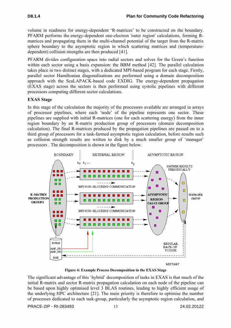
volume in readiness for energy-dependent ‘R-matrices’ to be constructed on the boundary. PFARM performs the energy-dependent one-electron 'outer region' calculations, forming R-matrices and propagating them in the multi-channel potential of the target from the R-matrix sphere boundary to the asymptotic region in which scattering matrices and (temperature-dependent) collision strengths are then produced [41].
PFARM divides configuration space into radial sectors and solves for the Green’s function within each sector using a basis expansion: the BBM method [42]. The parallel calculation takes place in two distinct stages, with a dedicated MPI-based program for each stage. Firstly, parallel sector Hamiltonian diagonalisations are performed using a domain decomposition approach with the ScaLAPACK-based code EXDIG. The energy-dependent propagation (EXAS stage) across the sectors is then performed using systolic pipelines with different processors computing different sector calculations.
EXAS Stage
In this stage of the calculation the majority of the processors available are arranged in arrays of processor pipelines, where each ‘node’ of the pipeline represents one sector. These pipelines are supplied with initial R-matrices (one for each scattering energy) from the inner region boundary by an R-matrix production group of processors (domain decomposition calculation). The final R-matrices produced by the propagation pipelines are passed on to a third group of processors for a task-farmed asymptotic region calculation, before results such as collision strength results are written to disk by a much smaller group of ‘manager’ processors . The decomposition is shown in the figure below.
Figure 4: Example Process Decomposition in the EXAS Stage
The significant advantage of this ‘hybrid’ decomposition of tasks in EXAS is that much of the initial R-matrix and sector R-matrix propagation calculation on each node of the pipeline can be based upon highly optimised level 3 BLAS routines, leading to highly efficient usage of the underlying HPC architecture [21]. The main priority is therefore to optimise the number of processes dedicated to each task-group, particularly the asymptotic region calculation, and

D8.1.4 Plan for Community Code Refactoring
PRACE-2IP - RI-283493 24.02.20122
14
minimise the runtime management (data collection) group whilst ensuring the best achievable load-balancing properties. The processor configuration is currently determined automatically via a Perl script using predictive algorithms for expected performance of each task-group [16], but this is in need of updating for the latest multi/many core and accelerator based architectures.
2.3.2 Performance Improvements
As described in the previous section, EXAS has been developed so that the vast bulk of the computation takes place within optimised LAPACK and BLAS routines. It is probably fair to assume that these specialised, usually vendor-optimised libraries will continue to be provided on any future architecture in PRACE, including library routines optimised for accelerator-based architectures. With this in mind, the key to enabling fast and scalable performance of EXAS lies with maintaining excellent load balancing and minimising initialisation, check-pointing and finalisation costs (all dependent upon efficient I/O).
Load-Balancing Model
The load-balancing model assigns the correct number of processes to each stage of the calculation (see Figure 4) in order that:
1. Initial R-matrices are produced at a sufficient rate to satisfy demand from the process pipelines
2. Asymptotic calculations are processed at a sufficient rate to deal with the supply of final R-matrices from the process pipelines
3. Pipelines are never stalled
The model is described in detail in [16] where the more complex ‘spin-split’ case is also modelled. It is used to calculate the number of process pipelines that can be formed from a given number of processes given that the computational load must be balanced with that of the other functional groups , , where is the number of processes in
the R-matrix production group, is the number of processes in the asymptotic region group
and is the number of processes in the manager group. For simplicity in this document
we assume a single R-matrix production group. The PFARM code has been upgraded for petascale architectures to allow several production groups working simultaneously with appropriate adjustment of the performance model. The model takes into account how the computational load varies for different group sizes, with two coefficients requiring adjustment according to hardware architecture and communication efficiency. These coefficients need to be obtained for each (PRACE) hardware system by test runs to be carried out as part of the porting process.
Based on standard floating point operation counts for matrix-matrix operations, it is straightforward to show that the number of floating point operations (flops) required to construct initial propagation R-matrices is:
2
where qin is the number of radial continuum basis functions retained in each channel in the internal region and n is the number of channels.

D8.1.4 Plan for Community Code Refactoring
PRACE-2IP - RI-283493 24.02.20122
15
The number of flops required to calculate a corresponding sector R-matrix in a pipeline is:
6
where q is the number of BBM basis functions retained in each channel in the external region.
A constant C1 is introduced to account for communication costs during propagation. This is machine dependent and varies according to factors such as memory bandwidth and latency, interconnect bandwidth and latency and the system’s efficiency in overlapping communication with computation.
Therefore the ratio can be written as
26
which reduces to
3
This determines the ratio of number of pipelines to processes in the initial R-matrix production group.
Similarly, at the end of each pipeline sufficient processes must be allocated to the asymptotic calculation group to prevent the pipelines from being held up.
Calculations on the asymptotic nodes are dominated by the singular value decomposition LAPACK routine dgesvd during the calculation of the K-matrix. The number of flops in the calculation is 12n3 when all channels are open. Therefore the ratio
: is:
126
Where C2 is a constant that arises from i) the proportion of the total time spent calculating the K-matrix in the overall asymptotic calculation (usually close to 1) and ii) the relative flop rate of dgemm and dgesvd.
Assembling these ratios and introducing , and , respectively the total number of processes, the number of processes in each pipeline and the number of manager nodes (all determined from the input data), gives us the following relationship for the non-spin-split case :
(where , , are estimated to the nearest integer).
Parallel I/O using ‘XStream’
In order for the models of the type described above to be highly accurate, the amount of time spent in setting up the production system and producing final data, in particular I/O from the internal region, between the EXDIG and EXAS stages and final output of what may be large amounts of energy and temperature dependent scattering data must be minimal. This is not necessarily the case for petascale HPC machines designed for clock-rate performance and for

D8.1.4 Plan for Community Code Refactoring
PRACE-2IP - RI-283493 24.02.20122
16
which substantial serial I/O may become a major architecture-dependent bottleneck. This question must be tackled by adopting parallel I/O methods that target relevant MPI tasks, do not overload the system and which ideally produce portable data, as for example, the inner and outer region stages may be run on different machines. We note the following points.
• R-Matrix codes consist of various stages (eg, radial integrals, angular couplings, Hamiltonian construction and diagonalization inner region stages, diagonalization and propagation/asymptotic PFARM outer region stages). The older serial codes used unformatted and direct access files to pass data: this is not always portable. More recently, final inner region output may be written in portable XDR format.
• PFARM preferably uses XDR files but may also read unformatted binary files in various convenient data arrangements to read inner region data, and XDR files between stages with data written to different files for pickup by the different groups in EXAS. MPI-IO files are more efficient in parallel but not portable.
• The I/O-handling ‘XStream’ package [46]. is being developed to provide a wrapper package to allow various option at any given file read/write. Details of the format required are supplied in a much more straightforward manner than the set of namelist parameters currently required: the package provides a generic interface for top-level I/O routines in order to provide effective object oriented parallel I/O. Internally an MPI-IO extension allows parallel writes and reads to different file records which follow the direct access patterns originally expected by the codes.
• The package is already in use in other (inner region) programs within the R-matrix suite.
• The final package will be freely available as a standalone to be incorporated into other codes in the PRACE project.
Conclusions
The workplan for PFARM will first allow detailed testing of the load-balancing performance models on the range of PRACE architectures, leading to fine-tuning (any necessary adjustments) and ideally a straightforward automated procedure and script to generate the machine dependent coefficients and optimal core distributions. It will also thoroughly upgrade and test the parallel XStream package to be useful as a general key I/O tool within PRACE, in addition to further improving the R-matrix suite. If time permits, a secondary goal will test any recent developments in parallel eigensolver library routines, such as ELPA [44] and MAGMA [45] in order to determine their suitability for the large Hamiltonian diagonalizations that are required in EXDIG.
2.3.3 Workplan
PFARM electron-atom electron-molecule collisions R-matrix Code Development
Implementation Testing and Optimization
Figure 5: GANTT chart for PFARM.

D8.1.4 Plan for Community Code Refactoring
PRACE-2IP - RI-283493 24.02.20122
17
Workplan Milestones:
M14: EXDIG Parallel IO completed
M18: EXAS Parallel IO completed
M20: XStream Final Package completed
2.3.4 Testing and Validation Procedure
During development of the parallel code results from a standard test suite were collected and regularly validated with results from the code’s predecessor - serial FARM and other propagation methods [47]. More recently an alternative R-matrix propagation code has been developed based on the Airy Log-Derivative propagator, originally developed by Alexander [48] which has allowed validation of larger test cases [46].

D8.1.4 Plan for Community Code Refactoring
PRACE-2IP - RI-283493 24.02.20122
18
3 Climate As discussed in deliverable 8.1.2 [3], seven codes were evaluated and analysed within four different areas of computational climate science:
1. Couplers: OASIS 2. Input/Output: CDI, XIOS, PIO 3. Dynamical cores: ICON 4. Ocean Models: NEMO, Fluidity-ICOM
The performance analysis reported in [3] and the potential computational improvements proposed in [4] led to extensive work for some of the codes, such as ICON, NEMO and Fluidity-ICOM, on porting to GPUs. In addition, performance models were developed for some of these codes and these results are also reported here. In the areas of couplers, preparatory work on analysing the scalability of OASIS3-MCT has taken place and is reported here. The effort on I/O was of preliminary nature, namely forging a consensus among I/O stakeholders in the community. The initial I/O strategy and work plan are discussed subsequently.
3.1 Couplers: OASIS
The OASIS coupler was seen to be a key component of European climate models, and its performance was shown in D8.1.2 to be a bottleneck to petascale and exascale modelling. In D8.1.3, a new version of OASIS, OASIS3-MCT, was examined and tested against OASIS4 with pre-computed weights. Following this, it has been decided to optimise OASIS3-MCT as the coupler for scaling current climate models, and prepare a new generation of coupler for future models.
OASIS3-MCT, combining the coupler from CERFACS with the Model Coupling Toolkit (MCT,[31]) was tested on the PRACE Tier-0 Bullx computer “CURIE” up to 2048 cores. As the code has been under active development, a full performance model has not been possible. Nevertheless, two scaling weaknesses were highlighted at high core counts:
1. The time taken to exchange fields in the “toyatm/ocn” test case with high resolution fields (IFS T799 grid and the ocean component using the ORCA 0.25 deg grid) was seen to decrease for 1 to 128 cores, but then increase. Profiling shows that while communications remain reasonable, the matrix-multiply when remapping from the source to target grid is responsible for the uptick in time taken. Hence this has been chosen as a target for optimisation.
Figure 6: OASIS3-MCT: Coupling exchange
0,0000
5,0000
10,0000
15,0000
20,0000
25,0000
30,0000
35,0000
1 4 16 64 256 1024
Datenreihen1Datenreihen2

D8.1.4 Plan for Community Code Refactoring
PRACE-2IP - RI-283493 24.02.20122
19
2. The time taken for initialisation of the coupler has been highlighted for work. While the time taken for initialisation is in practice a small part of the overall runtime of climate simulations, it may be significant in the case of multiple, short runs. Hence this was chosen as the second target for optimisation within PRACE WP8.
ICHEC will be dedicating 6 months of effort to these tasks.
Figure 7: time spent in OASIS3-MCT initialisation
Secondly it was agreed to work on developing the „next generation“ coupler, targeting models with icosahedral or unstructured grids (e.g. ICON, the Fluidity-ICOM ocean model, etc.). Open-PALM has been developed at CERFACS and ONERA for data assimilation in ocean models. While this coupler is frequently used in many fields, such as aerospace, it does not to date include conservative interpolation. Hence it is agreed to analyse using existing conservative interpolation schemes (e.g. ESMF and Farrell/Maddison) within Open-PALM. This work is to be undertaken by CEA/GENCI: the work will be done through „ La Maison de la Simulation“ by Joel Chavas, in collaboration with CERFACS. 12 months of effort will be devoted to this task.
Figure 8: GANTT chart for OASIS
3.2 Input/Output: CDI, XIOS, PIO
As described in D8.1.3 [4], a common “I/O services” module is being developed within the ENES community, for use by all climate models. A workshop is planned at DKRZ in Hamburg on February 27-28, 2012, at which the design will be completed. Hence full details of this task were postponed until this meeting. Nevertheless, progress has been made on the larger design of the proposed “IO services” module and the role of PRACE-2IP WP8:
I/O services will implement a writer service, reading data from the model nodes (those nodes running the climate model itself) via RDMA / single-sided communications. This enables the model to continue while I/O services handles the parallel write (read is not an issue for global models).
0,0000
20,0000
40,0000
60,0000
80,0000
100,0000
120,0000
140,0000
1 4 16 64 256 1024
Datenreihen1Datenreihen2

D8.1.4 Plan for Community Code Refactoring
PRACE-2IP - RI-283493 24.02.20122
20
The I/O services implement parallel writes to a number of potential formats, principally netCDF and GRIB, using the CDI library or a variant.
The I/O services are implemented using separate I/O nodes, to enable buffering of I/O in memory. This balances the large transient communications internal to the compute cluster (e.g. 250 GB/s) to the typically smaller but sustained I/O bandwidth; then I/O scaling becomes a matter of adding additional nodes for I/O.
Post-processing is then handled on the fly within the I/O services, based on the XIOS model from IPSL. This work is done in collaboration with IPSL (XIOS developers), MPI-M (CDI developers), in parallel to the G8 “ICOMEX” dycore initiative and IS-ENES efforts.
Within PRACE, ICHEC and CSCS will implement an initial template version of the common I/O services based on the ScaLES CDI, in comparison to the existing PIO developed at NCAR. This implements the API, in which the post-processing services will be implemented in parallel by ENES partners (IPSL).
Currently ICHEC are scheduled to do 18 months effort on this project; CSCS 6 M.
3.3 Dynamical Cores: ICON
3.3.1 Performance Model
As pointed out in deliverable D8.1.3 [4], the ICON non-hydrostatic dynamical core is a good candidate for the Roofline Model [15]. This semi-empirical model (see Figure 9) provides a simple, understandable mechanism for predicting performances on emerging architectures based on two simple benchmarks: the stream benchmark for attainable memory bandwidth, and a computationally intensive micro-benchmark (generally a matrix-matrix multiplication) to determine the maximum attainable floating-point performance. For a memory bandwidth-bound application, the rate of floating-point operations is related linearly to the computational intensity, namely the number of operations performed per byte transferred to/from memory (which may or may not reside in cache). At some given computational intensity, the floating-point unit becomes the bottleneck, and the performance saturates at roughly the micro-benchmark level.
As discussed in D8.1.3 [4], the computational intensities of the ICON NH kernels were the subject of an extensive evaluation at the beginning of the project. As shown in Figure 10, the intensities range from 0.1 to 1.0, with an average of 0.38. ICON NH performs exclusively double precision (8-byte) arithmetic.

D8.1.4 Plan for Community Code Refactoring
PRACE-2IP - RI-283493 24.02.20122
21
Figure 9: The Roofline Model provides a simple mechanism for predicting application performance based on two benchmarks. The performance figures given are for a quad-core Opteron 8380 (2.5 GHz).
Figure 10 : The roughly 60 ICON NH kernels vary in computational intensity and performance. The outlying kernels on the right and left are part of the vertical implicit solver, which has loop dependencies and has to run sequentially, noticeably reducing performance.
In order to predict the time to solution of the dynamical core, we take note of the following attributes of ICON NH:
As one would expect, run time is linear in the number of iterations. The base resolution, R2B0 with 80 triangles and 35 vertical levels, requires roughly
0.0735 giga-operations (GFlop) per iteration. The step from one iteration level to the next higher consists of subdividing each
triangular face into four new triangles, and adds almost exactly a factor of 4 to the

D8.1.4 Plan for Community Code Refactoring
PRACE-2IP - RI-283493 24.02.20122
22
number of operations. Tests show that run times on CPUs increase by slightly larger factor (4.1-4.2) probably due to cache effects. On GPUs, the run times increase by a factor of less than four due to better utilisation of the device (higher thread occupancy).
This leads to the following prediction of time to solution (in seconds), as a function of the number of iterations, the level of refinement, and the memory bandwidth (in GB/s) determined from the stream benchmark:
Some single-node measured triad-stream benchmarks are: 45.9 GB/s on a dual-socket AMD Interlagos (32 total cores) node, 24.8 GB/s on a single socket Intel Westmere (8 cores), 116.6 GB/s on an NVIDIA GTX285, 84.1 GB/s on an NVIDIA S1070, and 103.1 GB/s on an NVIDIA C2070.
This model is oblivious to cache issues, and assumes, in the case of GPUs, that all data are moved to the device before the first time iteration and copied back after the last. Figure 11 contains the predicted and measured execution times for 1000 iterations of the ICON NH dynamical core. The single-node model provides good predictions on the AMD Interlagos and NVIDIA Fermi C2070 architectures. On the NVIDIA GTX285 and Tesla S1070, the actual timings are more than twice the predicted, however these are expected, due to known performance issues with double precision arithmetic. The Intel Westmere performs considerably better than predicted, most likely due to better cache utilisation than the AMD Interlagos.
Figure 11: Predicted and measured single-node ICON-NH execution times for R2B3 and R2B4 resolution (1000 iterations)
The performance modelling so far has concentrated on single-node implementations. The current ICON development code is, however, an MPI+OpenMP hybrid code. Single-node optimisation is a mute point if communication – mainly the halo exchange – is the fundamental bottleneck. We have therefore performed a preliminary analysis of node-to-node communication, to determine the node configuration where communication starts to dominate. Figure 12 indicates that R2B4 communication is manageable until at least 4 nodes, and R2B5 communication until 8 nodes, and higher resolutions should scale out farther. It is clear that one should run the application on the minimal number of nodes, filling up the node
t(lev,iter,bmax ) 0.00735 iter 4 lev
0.38 bmax
0
20
40
60
80
100
120
140
160
180
200
Interlagos 32 cores
Westmere 8 cores
GeForce GTX 285
Tesla S1070 Fermi C2070
Time (s.)
Platform
R2B3 Predicted
R2B3 Measured
R2B4 Predicted
R2B4 Measured

D8.1.4 Plan for Community Code Refactoring
PRACE-2IP - RI-283493 24.02.20122
23
memory as much as possible. On the other hand, strong scaling to large configurations cannot be expected.
Figure 12: The aggregated time for computation (blue) and communication (red), for R2B4 and R2B5 on a Cray XK6 with 16 cores per node. Optimal scaling would yield horizontal lines. Green (AMD Interlagos), purple (Intel Westmere) and light blue (NVIDIA M2090) indicate the predicted times for those architectures assuming optimal scaling, and these timings are therefore a worst-case scenario for communication.
3.3.2 Testing and Validation
From the initial case study, the test harness for the single-node implementation is available for testing correctness of GPU kernel results to those on the CPU. While bit-for-bit identity between CPU and GPU is generally not achievable, a round-off tolerance can be defined. These round-off acceptance tests should be sufficient for the development of the directive-based port to GPUs, however, a final validation of the model running on GPU and/or CPU must still be performed by the community (e.g., MPI-M). As ICON is still under development, such a validation will take place in any case.
3.3.3 Work Plan
The basic community requirement for the ICON hydrostatic and non-hydrostatic dynamical cores is a portable code, which performs well on current and future architectures. Moreover, the long-term goal is to formulate the underlying algorithms with a domain specific language (DSL). PRACE views its contribution to these goals as (1) providing efficient underlying implementations for emerging technologies (e.g., GPUs, MIC, Sandybridge), without sacrificing performance on current ones, (2) supplementing existing efforts to look at new DSL paradigms which might be applicable for this purpose, and (3) investigating parallel I/O strategies. As parallel I/O will be discussed in a separate section, only two central objectives are defined here for the remainder of the project:
Task A: A performance-portable implementation of the kernels constituting the ICON NH dynamical core. This will be based on the existing code, augmented with additional OpenMP and OpenACC directives to support both CPUs and GPUs.
Task B: A prototype implementation of a scaled-down ICON dynamical core based on the OP2 [56] domain-specific language for unstructured-mesh CFD problems.
The key personnel in this effort are:
Task A: Max Planck Institute for Meteorology, L. Linardakis, et al.; Swiss National Supercomputing Centre, W. Sawyer, G. Fourestey
Task B: Imperial College, D. Ham, C. Bertolli; The Cyprus Institute, G. Fanourgakis
The following milestones are proposed:
M9, Task A: proposal for the multi-platform design which offers suggestions how to incorporate multiple programming paradigms (e.g., OpenMP, OpenACC, possibly CUDA or OpenCL) into one code base while maintaining performance portability
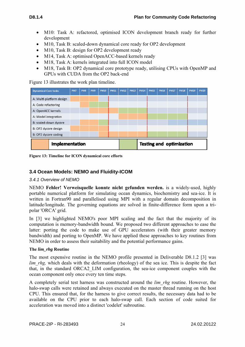
D8.1.4 Plan for Community Code Refactoring
PRACE-2IP - RI-283493 24.02.20122
24
M10: Task A: refactored, optimised ICON development branch ready for further development
M10, Task B: scaled-down dynamical core ready for OP2 development M10, Task B: design for OP2 development ready M14, Task A: optimised OpenACC-based kernels ready M18, Task A: kernels integrated into full ICON model M18, Task B: OP2 dynamical core prototype ready, utilising CPUs with OpenMP and
GPUs with CUDA from the OP2 back-end
Figure 13 illustrates the work plan timeline.
Figure 13: Timeline for ICON dynamical core efforts
3.4 Ocean Models: NEMO and Fluidity-ICOM
3.4.1 Overview of NEMO
NEMO Fehler! Verweisquelle konnte nicht gefunden werden. is a widely-used, highly portable numerical platform for simulating ocean dynamics, biochemistry and sea-ice. It is written in Fortran90 and parallelised using MPI with a regular domain decomposition in latitude/longitude. The governing equations are solved in finite-difference form upon a tri-polar 'ORCA' grid.
In [3] we highlighted NEMO's poor MPI scaling and the fact that the majority of its computation is memory-bandwidth bound. We proposed two different approaches to ease the latter: porting the code to make use of GPU accelerators (with their greater memory bandwidth) and porting to OpenMP. We have applied these approaches to key routines from NEMO in order to assess their suitability and the potential performance gains.
The lim_rhg Routine
The most expensive routine in the NEMO profile presented in Deliverable D8.1.2 [3] was lim_rhg, which deals with the deformation (rheology) of the sea ice. This is despite the fact that, in the standard ORCA2_LIM configuration, the sea-ice component couples with the ocean component only once every ten time steps.
A completely serial test harness was constructed around the lim_rhg routine. However, the halo-swap calls were retained and always executed on the master thread running on the host CPU. This ensured that, for the harness to give correct results, the necessary data had to be available on the CPU prior to each halo-swap call. Each section of code suited for acceleration was moved into a distinct 'codelet' subroutine.

D8.1.4 Plan for Community Code Refactoring
PRACE-2IP - RI-283493 24.02.20122
25
All unnecessary data transfers to and from the GPU were eliminated by making the related variables 'resident' on the device. Required data transfers for these variables were then explicitly managed via HMPP's advancedload/delegatedstore directives. Note that trying to declare Fortran allocatable arrays to be resident on the GPU revealed a bug in HMPP (version 2.4.4). For the purposes of the test harness therefore, these allocatable arrays were made static.
As with the majority of NEMO, the computational intensity of the loops in lim_rhg is actually rather low. In addition, the sea-ice model does not use an explicit discretisation of the thickness of the ice and as a result there is no z-dimension to the calculations. Hence all of the compute loops are only doubly nested.
Nehalem CPU
Tesla GPU
Region Call count Total (s) Total (s)
Whole kernel 6 39.43 981.04
Alloc GPU 2 0.00 2.43
GPU store 3252 0.00 273.41
GPU load 2172 0.00 179.75
part1 6 0.22 4.43
part2 6 0.35 7.60
part3a 720 12.94 9.11
part3b 720 4.23 7.40
part3c 720 5.86 6.15
part3d_odd 360 2.63 129.92
part3d_even 360 2.73 130.74
part3e_even 360 2.65 133.89
Table 3: Comparison of the profiles of the ported lim_rhg routine when run on a single Nehalem core and a Tesla GPU. Only codelets, data transfer and GPU initialisation costs are included. Timings are for the ORCA025 grid.
The profile of the ported, optimised lim_rhg routine for an ORCA025-resolution test case is shown in Table 3 for both a single Nehalem core and a Tesla GPU. Clearly the average time taken per kernel call is much greater on the GPU (164 s) than it is on the Nehalem (7 s). However, this large difference is primarily due to data transport costs as can be seen by the entries for GPU store and GPU load (data downloaded from the GPU to CPU RAM and vice versa, respectively). The part3d* and part3e* kernels also include substantial data transfer costs because their codelet arguments include arrays that are transferred to/from the GPU upon every call. (They have not been optimised to the same extent as the other kernels in the table.) This emphasises the need to optimise data transport to/from the device in order to achieve good overall performance.

D8.1.4 Plan for Community Code Refactoring
PRACE-2IP - RI-283493 24.02.20122
26
In this case however, the compute performance itself does not justify the effort required to optimise the data transport. Consider the performance of the part3a-c kernels, which are particularly important due to their involvement in the iterative solver (note the high call counts). Only for part3a does the GPU out-perform the Nehalem core and then only by ~30%; part3b is ~75% slower on the GPU and part3c ~5% slower. This is to be contrasted with the situation in tra_ldf_iso (below) where the kernel was a factor of four faster on the Tesla GPU and retained a factor of two speed-up, even when OpenMP was employed to use all four cores of a single Nehalem chip.
We can therefore conclude that given the low performance of the compute kernels and the frequency with which data must be transferred back to the CPU memory, this routine is not well suited to making good use of the Tesla GPU.
The tra_ldf_iso routine
Before attempting to optimise the routine for the GPU, we measured its performance on a single core of an Intel Nehalem chip. Compiled with the Intel compiler with flags ``-O3 -axAVX'' and run on 1 Nehalem core the mean time/kernel call over 100 calls was 0.095 seconds. Following all of the optimisations done for the GPU, this time was reduced to 0.082 seconds. The most difficult task in porting the kernel was dealing with the scoping of the various arrays used in the computation; with the exception of integer parameters, all of the variables used in an accelerated region must be contained within the current program unit and cannot come from external modules.
We worked around this issue by enclosing the computational kernel (the body of a subroutine that USE'd several modules) within a 'region' pragma. The data usage patterns for the various arrays (c.f. INTENT(in) or INTENT(inout) in Fortran) are then specified as parameters to the region. The key steps in optimising the resulting kernel are listed in Table 4.
Optimisation notes No. of calls Mean time per call (s)
First working traldf_iso on GPU 10 32.238
Put !$hmppcg parallel for outer two loops of the most expensive triply-nested loop
10 16.920
Repeat above for all triply-nested loops 10 0.100
Move outer tracer loop inside and unroll 10 0.100
Put io=in condition on temporary arrays to prevent them being copied back to host
10 0.096
Simulate 3D gridification in 2D on most expensive loop
100 0.067
Permute indices (jk, jj, ji) to (jj, ji, jk) on second most expensive loop
100 0.053
Undo 3D gridification on most expensive loop and permute indices
100 0.022

D8.1.4 Plan for Community Code Refactoring
PRACE-2IP - RI-283493 24.02.20122
27
Permute indices on all remaining loops 100 0.017
Removal of device allocation from within timing region
100 0.015
Optimised code on single Nehalem core 100 0.082
Table 4: The key stages in optimising tra_ldf_iso to run on the Tesla GPU using HMPP workbench. For comparison, the bottom row gives the performance of the final code when built with the Intel compiler and run on a single core of a Nehalem chip.
As with the PGI directives, the key step is, unsurprisingly, to ensure that the correct loops are being parallelised. The next largest improvement was gained by permuting loop indices from (jk,jj,ji) (i.e. levels, latitude, longitude) to (jj,ji,jk). If left unpermuted, the nested loop is parallelised such that consecutive threads are working on array sections well separated in memory. Since threads on the GPU are divided up into groups which are then executed in lock-step/SIMD (Single Instruction Multiple Data) fashion, best performance is obtained when a fetch from memory supplies data that can be used by all of the threads in a given group. If the threads aren't working on a contiguous section of memory then this will not happen. Permuting the loop indices ensures that parallelisation occurs over the indices in which an array is contiguous in memory and thus that neighbouring threads are working on contiguous parts of an array. The final result of 0.015 s per kernel call is some 20% faster than the time of 0.021 s achieved with the PGI directives.
The tra_adv_tvd routine
The tra_adv_tvd routine calls another subroutine, nonosc, but the two routines combined are only 374 lines in total. However, both tra_adv_tvd and nonosc contain several halo-swap calls and these present the major difficulty in porting these routines to the GPU.
As with the other routines, we first created a serial test harness for tra_adv_tvd which allows its results to be compared with those obtained from the original version within NEMO. The initial form of this harness with the original version of tra_adv_tvd demonstrated that it took 0.115 s/call on a single Westmere core and 0.124 s/call on a single Nehalem core (when compiled with the Intel compiler with “-O3 -axAVX”).
We used HMPP Workbench to port the routine due to its support for asynchronous data movement. Since the calls to the halo-swap routines must be executed on the CPU, these naturally break the routine up into several sections, each of which was made into a separate codelet for execution on the GPU. The two calls to nonosc had to be inlined since code executing on a GPU cannot call subroutines within the HMPP model. In total the ported routine consists of six codelets for execution on the GPU. As usual, great care had to be taken to avoid unnecessary data transfers to/from the GPU. For this we made use of HMPP's ability to map an array from different codelets to the same piece of memory on the GPU and keep it there between calls. This achieves the same result as declaring an array to be device-resident but is simpler to do in practice. We also succeeded in removing uploads/downloads of temporary arrays by declaring them as inputs to the codelet and then using the noupdate clause for them at the corresponding callsite.
The main steps in the porting and optimisation of the routine are listed in Table 5. After significant effort, the final, ported version of the routine on a Tesla GPU is some 31% faster than the original version running on a Nehalem core when using the ORCA2_LIM dataset. Attempts to execute the code with the ORCA025 grid failed because of insufficient memory on the GPU and so we used the ORCA1 grid.

D8.1.4 Plan for Community Code Refactoring
PRACE-2IP - RI-283493 24.02.20122
28
Notes Time per call (s)
First working port with kernel1 on GPU 0.401
Permute loops in kernel1 0.229
Move kernel2 to GPU 0.252
Permute loops in kernel2 and keep arrays on GPU between calls 0.214
Make kernel2 asynchronous and overlap with halo swaps 0.194
Asynchronous download of results from kernel2 0.177
In-line nonosc and convert into two codelets, nonosc1 and nonosc2 0.274
Permute loops in nonosc{1,2} 0.242
Make work arrays in nonosc{1,2} local instead of arguments. Overlap sending of work arrays with their halo swaps.
0.205
Remove unnecessary data transport for nonosc{1,2} 0.196
Move kernel3 to GPU 0.181
Improve halo-swap performance by re-ordering indices on work arrays so that tracer index is slowest-varying
0.092
Move working-array initialisation into separate kernel_init so can overlap with data transfers which must happen upon every iteration of the timing loop (more realistic)
0.095
Re-ordered initial data loads and switched to have them synchronous and kernel_init codelet asynchronous
0.085
Original kernel on single Nehalem core 0.124
Table 5: Steps in the porting and optimisation of the tra_adv_tvd routine. Timings are on Nehalem and Tesla hardware for the ORCA2 dataset.
Figure 14 shows the breakdown of the kernel execution time in terms of compute and data transport (to and from the GPU). From a comparison of the first two columns, it is clear that data transport is the main performance bottleneck when the kernel is run on the GPU. However, the majority of the data transfers between the GPU and CPU are for the purposes of doing halo-swaps which obviously only involves the halo regions of each array. Therefore, we modified the code so that only the halo regions of an array are transferred between the GPU and CPU when doing a halo swap. Doing so reduced the time spent in transferring data from 0.34 s (per kernel call) to just 0.09 s when using the Tesla GPU (third bar in Figure 14). Uploads (downloads) of halos to (from) the GPU were overlapped with the packing (unpacking) of halos on the CPU for any other arrays involved in a particular halo swap.

D8.1.4 Plan for Community Code Refactoring
PRACE-2IP - RI-283493 24.02.20122
29
Figure 14: Time spent in compute and data transport in the tra_adv_tvd kernel for the ORCA1 grid when running on a single Nehalem (Westmere) core and a Tesla (Fermi) GPU. The 2nd bar shows performance before halo transfers were optimised.
Finally, this version of the kernel was benchmarked on a Fermi GPU. As expected, the data transport cost remained similar at 0.08 s per call and the computational cost was slightly reduced from 0.14 s on the Tesla to 0.11 s on the Fermi. Strangely, this time was obtained when the NVIDIA CUDA compiler targeted the Tesla architecture (``sm_13''). If it targeted the Fermi (``sm_20'') architecture then the computational cost of the resulting binary was 0.13 s per kernel call (see the rightmost two bars in Figure 14).
OpenMP
Finally, for a fair comparison of the performance of the GPU with the CPU we must create a version of the GPU-accelerated routine capable of using all of the cores on the CPU. The standard method for doing this is to use OpenMP to parallelise the various loops in the routine over the available number of threads/cores. In order to minimise the overhead of the creation and destruction of thread teams, the whole timing loop was enclosed within an OMP PARALLEL region. Within this, each computational loop was parallelised by simply specifying OMP DO. This means that all of the 3D loops were parallelised in the z/depth dimension. The few 2D loops, mainly dealing with the surface and ocean floor, were parallelised in the y dimension.
In order to maintain good performance when running across more than one socket, the code had to be modified to ensure that memory was initialised by the thread that will access it, rather than just by the master thread - this ensures that it is allocated in close vicinity to the physical core on which it is executing. Care also must be taken in enforcing suitable affinity settings in the run-time environment. We set KMP_AFFINITY=none and used the taskset command on the linux-based systems and set PSC_OMP_AFFINITY=FALSE on HECToR. On the Westmere chip, the six- and four-thread jobs were fastest when the threads were shared evenly between the two sockets of a node. (This demonstrates that four threads are sufficient to saturate the memory bandwidth to a single socket.) On the older Nehalem chip, the same applied just to the four-thread job. We were unable to find any way to guarantee the sharing of threads evenly between sockets on the Power7 system.
Porting tra_ldf_iso with OpenMP
Figure 15 shows the performance of the OpenMP version of tra_ldf_iso relative to the HMPP version running on the NVIDIA Tesla card. For a single thread/core, the Intel Nehalem and Westmere processors gave very similar performance and were, surprisingly, slightly quicker
Nehalem Tesla (whole arrays) Tesla sm_20, Fermi sm_13, Fermi0
0.1
0.2
0.3
0.4
0.5
0.6
0.7
Compute Transport
Tim
e p
er k
ern
el c
all
(s)
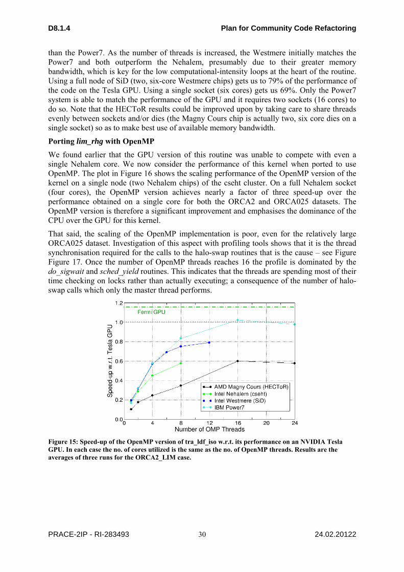
D8.1.4 Plan for Community Code Refactoring
PRACE-2IP - RI-283493 24.02.20122
30
than the Power7. As the number of threads is increased, the Westmere initially matches the Power7 and both outperform the Nehalem, presumably due to their greater memory bandwidth, which is key for the low computational-intensity loops at the heart of the routine. Using a full node of SiD (two, six-core Westmere chips) gets us to 79% of the performance of the code on the Tesla GPU. Using a single socket (six cores) gets us 69%. Only the Power7 system is able to match the performance of the GPU and it requires two sockets (16 cores) to do so. Note that the HECToR results could be improved upon by taking care to share threads evenly between sockets and/or dies (the Magny Cours chip is actually two, six core dies on a single socket) so as to make best use of available memory bandwidth.
Porting lim_rhg with OpenMP
We found earlier that the GPU version of this routine was unable to compete with even a single Nehalem core. We now consider the performance of this kernel when ported to use OpenMP. The plot in Figure 16 shows the scaling performance of the OpenMP version of the kernel on a single node (two Nehalem chips) of the cseht cluster. On a full Nehalem socket (four cores), the OpenMP version achieves nearly a factor of three speed-up over the performance obtained on a single core for both the ORCA2 and ORCA025 datasets. The OpenMP version is therefore a significant improvement and emphasises the dominance of the CPU over the GPU for this kernel.
That said, the scaling of the OpenMP implementation is poor, even for the relatively large ORCA025 dataset. Investigation of this aspect with profiling tools shows that it is the thread synchronisation required for the calls to the halo-swap routines that is the cause – see Figure Figure 17. Once the number of OpenMP threads reaches 16 the profile is dominated by the do_sigwait and sched_yield routines. This indicates that the threads are spending most of their time checking on locks rather than actually executing; a consequence of the number of halo-swap calls which only the master thread performs.
Figure 15: Speed-up of the OpenMP version of tra_ldf_iso w.r.t. its performance on an NVIDIA Tesla GPU. In each case the no. of cores utilized is the same as the no. of OpenMP threads. Results are the averages of three runs for the ORCA2_LIM case.

D8.1.4 Plan for Community Code Refactoring
PRACE-2IP - RI-283493 24.02.20122
31
Figure 16: Scaling performance of the OpenMP version of the lim_rhg kernel on a Nehalem compute node for the ORCA2 and ORCA025 datasets.
Figure 17: Profile of the OpenMP version of the lim_rhg kernel as the number of OpenMP threads is increased. Results are for the ORCA2 dataset run on HECToR IIb.
Future Strategy
The performance of the kernels discussed here on both GPU and CPU combined with the amount of work/changes to the source code required to port to GPU strongly suggests that it is worth pursuing the use of OpenMP within NEMO rather than continue porting to GPU. The ocean code ROMS and atmospheric code WRF both use a “coarse-grain” approach to OpenMP parallelism. In this technique, the section of the simulation domain allocated to each MPI process is further subdivided into a (configurable) number of 'tiles' that are then distributed amongst the OpenMP threads. The number of tiles need not be the same as the number of threads. This scheme has been shown [55] to be essential for WRF to scale well as the number of cores per node on a machine is increased.
NEMO Consortium member Centro Euro-Mediterraneo per i Cambiamenti Climatici (CMCC) have previously introduced OpenMP parallelism over the vertical levels in a model configuration used to study the Mediterranean Sea. As part of their work for the NEMO Consortium in 2012 they are planning to extend this work by parallelising the longitude/latitude dimensions with OpenMP. This work will be done on version 3.4 of NEMO, due for release in February 2012.
1 2 4 8 16 240
10
20
30
40
50
60
70
80
90
100
otherdo_sigwaitsched_yielddefgu2sdlbc_lnk_2dpart3e_evenpart3d_oddpart3d_evenpart3cpart3bpart3alim_rhg
Number of threads
Per
centa
ge o
f ru
n-t
ime

D8.1.4 Plan for Community Code Refactoring
PRACE-2IP - RI-283493 24.02.20122
32
We therefore propose to extend the NEMO test harness developed so far to use the coarse-grained approach to OpenMP parallelism. The design for this implementation will be done in collaboration with CMCC to avoid duplication of effort.
At present, all 3-dimensional fields in NEMO are stored in arrays such that the longitude index varies contiguously in memory, e.g. field(ii, jj, kk) where ii is the longitude index, jj is the latitude index and kk is the depth index (recall that NEMO is a Fortran code). Since the model uses a domain decomposition in latitude/longitude, this scheme means that as the number of processes/threads is increased, the size of the contiguous regions of memory that they have to work on decreases. On modern CPUs that rely on memory caching and vectorisation, this really damages performance. We will therefore implement a version of the test harness where the array indices are permuted such that the depth index varies contiguously in memory. In this approach, even if the number of OpenMP threads matches the number of ocean points in a domain, each of them will still have a column of ocean to work on which should improve scalability of the code. We will test this by comparing with the hybrid version of NEMO produced by CMCC where original array index ordering is retained.
Testing and Validation Procedure
The test harnesses developed so far compare the computed output of a subroutine with that produced by the original code running within NEMO for the ORCA2_LIM configuration (which is a part of the standard NEMO distribution). We also propose to begin testing with the regional AMM configuration, due to be released with version 3.4 of NEMO. These tests will include model stability as well as comparison of final output fields such as sea surface temperature and sea surface height.
3.4.2 Work plan (NEMO)
STFC will spend six person-months effort on NEMO in this part of the work package. Note that this 2nd phase of WP8.1 runs over 14 months from 01/03/2012 until 30/04/2013.
Work plan:
7 8 9 10 11 12 13 14 15 16 17 18 19 20
Effort
Milestones MS1 MS2 MS3
Where the project milestones are:
Milestone Date Description
MS1 End of M 7 Design coarse-grain OpenMP implementation in consultation with CMCC.
MS2 End of M 13 Complete implementation in test harness with array indices ordered level-index first.
MS3 End of M 20 Performance comparison with version from CMCC with standard array index ordering.
3.4.3 Fault-Tolerant NEMO
As systems move to exascale, it is important that climate models become fault-tolerant. At CERFACS work has started on a fault-tolerant implementation of NEMO. This is designed to survive failures in the MPI communications and node failures during runs. A fault tolerant

D8.1.4 Plan for Community Code Refactoring
PRACE-2IP - RI-283493 24.02.20122
33
version of MPI, OpenMPI-FT is being developed, which enables MPI runs to tolerate node failures, but NEMO needs to be adapted to use these features.
Within PRACE-2IP WP8, IPB will work to describe a strategy to repair communications after failure of one or several NEMO ocean model MPI-connected subdomains, ensure downgraded calculations on remaining resources and re-create missing information on failed subdomain area variables during the standard checkpoint/restart procedure.
Figure 18: GANTT chart for Fault Tolerant NEMO
3.4.3 Overview of Fluidity-ICOM
Fluidity-ICOM [49] is an open source partial differential equation simulator build upon various finite element and finite volume discretisation methods on unstructured anisotropic adaptive meshes It is being used in a diverse range of geophysical fluid flow applications. Fluidity-ICOM uses three languages (Fortran, C++, Python) and uses state-of-the-art and standardised 3rd party software components whenever possible.
The change of shifting from using faster processors to using multi-core processors is as disruptive to scientific software as the shift from vector to distributed memory supercomputers decades ago. The shift to multi-core systems will require applications to exploit many more fine-grain level parallelisms and overcome significant reductions in the bandwidth and volume of memory available to each CPU. This “scalability challenge” driven by the exponential increase in the amount of parallelism in the system affects all aspects of the use of high performance computing.
For modern supercomputers with NUMA nodes, hybrid OpenMP/MPI offers new possibilities for optimisation of numerical algorithms beyond pure distributed memory parallelism. For example, scaling of algebraic multigrid methods is hampered when the number of subdomains is increased due to difficulties coarsening across domain boundaries. The scaling of mesh adaptivity methods is also adversely effected by the need to adapt across domain boundaries.
Previous performance analysis [3] has already shown that the two dominant simulation costs are sparse matrix assembly (30%-40% of total computation), and solving the sparse linear systems defined by these equations. The Hypre library’s hybrid sparse linear system solvers/preconditioners, which can be used by Fluidity-ICOM through the PETSc interface, are competitive with the pure MPI implementation [4]. Therefore, in order to run a complete simulation using OpenMP parallelism, the sparse matrix assembly kernel is now the most important component remaining to be parallelised using OpenMP. The finite element matrix assembly kernel is expensive for a number of reasons including: significant loop nesting, where the innermost loop increases in size with increasing quadrature; many matrices have to be assembled, e.g. coupled momentum, pressure, free-surface and one of each advected quantity; indirect addressing (a known disadvantage of finite element codes compared to finite

D8.1.4 Plan for Community Code Refactoring
PRACE-2IP - RI-283493 24.02.20122
34
difference codes); and cache re-use (a particularly severe challenge for unstructured mesh methods).
For a given simulation, a number of different matrices need to be assembled, e.g. continuous and discontinuous finite element formulations for velocity, pressure and tracer fields for the Navier-Stokes equations and Stokes flow. Each of these have to be individually parallelised using OpenMP. Parallelism can be realised through well-established graph colouring techniques, where the graph defines the data dependencies in the matrix assembly. This approach removes data contention, so called critical sections in OpenMP, allowing very efficient parallelisation.
The current procedure for constructing sparse matrices in Fluidity uses an element-by-element approach. This is the case for all the different matrices assembled e.g. continuous Galerkin (CG), discontinuous Galerkin (DG), continuous volume (CV) and higher order finite element formulations. Sparse matrices are stored in PETSc’s CSR containers (these includes block-CSR for use with velocity vectors for example and DG) in order to avoid unnecessary memory-memory data copies, or having to write specialised matrix-vector operator call back routines. While the general principle behind threading finite element assembly using colouring will remain the same, the implementation details will change. In particular, the data dependency graph for different finite element formulations will change significantly. For example, while the data dependencies in DG advection are only between the nodes local to that element and those on the matching face of the adjacent elements, different diffusion operators can have much wider data dependencies. Thus, the first stage of the work is to itemise each of the formulations in use and construct their data dependency graphs.
To parallelise matrix assembly using colouring, a loop over colours is first added around the main assembly loop. The main assembly loop over elements will be parallelised using the OpenMP parallel directives with a static schedule. This will divide the loop into chunks of size ceiling (number_of_elements/number_of_threads) and assign a thread to each separate chunk. Within this loop an element is only assembled into the matrix if it has the same colour as the colour iteration.
3.4.5 Performance improvement.
While improving I/O is not a direct objective of this work plan, significant benefit can be expected from using mixed-mode parallelism. For example, only one process per node will be involved in I/O (in contrast to the pure MPI case where potentially 24 processes per node could be performing I/O on Phase 2b of HECToR), which will significantly reduce the number of metadata operations on the file system at large process counts. In addition, the total size of the mesh halo increases with number of partitions (i.e. number of processes). It can be shown empirically that the size of the vertex halo in a linear tetrahedral mesh grows as O(P1.5), where P is the number of partitions. Therefore, the use of hybrid OpenMP/MPI will decrease the total memory footprint per compute node, the total volume of data to write to disk, and the total number of metadata operations given Fluidity’s files-per-process I/O strategy.
The momentum equation assembly kernel using Discontinuous Galerkin methods (DG) has been parallelised with the above-mentioned procedures. Several thread safe issues have been solved which result of a performance gain.
Local assembly v.s. nonlocal assembly
In PETSc, when adding elements to a matrix, a stash is used. For parallel matrix formats this provides one particularly important benefit, namely that elements can be added in one process that are to be stored as part of the local matrix in a different process. During the assembly

D8.1.4 Plan for Community Code Refactoring
PRACE-2IP - RI-283493 24.02.20122
35
phase the stashed values are moved to the correct processor. We name it as nonlocal assembly, which causes thread safe issues within the momentum_dg assembly loop.
Luckily, when parameter MAT_IGNORE_OFF_PROC_ENTRIES is set, any MatSetValues accesses to rows that are off-process will be discarded, and the needed value will be computed locally, named by local assembly. Figure 19 shows that local matrix assembly is much faster than nonlocal assembly as no communications are needed. This makes assembly an inherently local process, therefore we can focus on optimising local (to the compute node) performance.
Figure 19: Speedup comparison between matrix local assembly and nonlocal assembly
Thread Safe Issues of Memory Reference Counting
For any defined type objects in Fluidity being allocated or deallocated, the reference count will be plus one or minus one. If the objects counter equals zero, the objects should then be deallocated. In general, the element-wise physical quantities should not perform allocation or deallocation in the element loop, but this is not the case in the kernels. The solution could be to either add critical directives around reference counter or move allocation or deallocation outside of element loop. We have implemented both solutions and performance comparison has been made in Figure 20. The results show that the mutual synchronisation directives (eg. ‘critical’) should be avoided. Moving allocation or deallocation outside of element loop has also improved the pure MPI version’s performance (see 24M1T in Figure 20).
Optimisation of memory bandwidth
One of the key performance considerations for achieving performance on ccNUMA nodes is memory bandwidth. In order to optimise memory bandwidth, the following methods have been employed to ensure good performance:
First-touch initialisation ensures that page faults are satisfied by the memory bank directly connected to the CPU that raises the page fault;
Thread pinning to ensure that individual threads are bound to the same core throughout the computation.

D8.1.4 Plan for Community Code Refactoring
PRACE-2IP - RI-283493 24.02.20122
36
Figure 20: Comparison between using critical directive and without critical directive
Thread pinning has been used through Cray aprun with all benchmarking tests. Compared the 12-thread runs, the time has been reduced from 45.127 seconds to 38.303 seconds after applying the first-touch policy. But even after applying the first-touch policy, there is still a sharp performance drop from 12 threads to 24 threads. This problem has been investigated by profiling with CrayPAT (Table 6).
Samp% | Samp | Imb. | Imb. |Group | | Samp | Samp% | Function | | | | PE=HIDE 100.0% | 75471 | -- | -- |Total |--------------------------------------------------------------------------------------------- | 95.8% | 72324 | -- | -- |ETC ||-------------------------------------------------------------------------------------------- || 14.6% | 11002 | 0.00 | 0.0% |_int_malloc || 13.8% | 10417 | 0.00 | 0.0% |__lll_unlock_wake_private || 9.7% | 7284 | 0.00 | 0.0% |free || 9.5% | 7172 | 0.00 | 0.0% |__lll_lock_wait_private || 6.4% | 4862 | 0.00 | 0.0% |malloc || 6.2% | 4674 | 0.00 | 0.0% |__momentum_dg_MOD_construct_momentum_element_dg || 4.0% | 3046 | 0.00 | 0.0% |_int_free || 3.2% | 2439 | 0.00 | 0.0% |__momentum_dg_MOD_construct_momentum_interface_dg || 3.0% | 2272 | 0.00 | 0.0% |_gfortran_matmul_r8 || 3.0% | 2251 | 0.00 | 0.0% |__sparse_tools_MOD_block_csr_blocks_addto || 2.8% | 2090 | 0.00 | 0.0% |malloc_consolidate || 2.1% | 1574 | 0.00 | 0.0% |__fetools_MOD_shape_shape Table 6 CrayPAT sample profiling statistic
The culprit appears to be the use of fortran automatic arrays in the Momentum_DG assembly kernel for support of p-adaptivity. There are a lot of such arrays in the kernel. Since the compiler can't predict its length, it allocates the automatic arrays on the heap. The problem is solved by using the NUMA-aware heap memory manager tcmalloc from gperftools [50], which makes pure OpenMP version’s performance better than pure MPI version within compute node. The speedup of 24 threads is 18.46 compared with using 1 thread for the Momentum_DG kernel.

D8.1.4 Plan for Community Code Refactoring
PRACE-2IP - RI-283493 24.02.20122
37
Conclusions
The Momentum_DG has been parallelised with OpenMP successfully. The above results indicate that node optimisation can be done mostly using OpenMP with the efficient colouring method. Improving memory bandwidth usage through NUMA optimisations (eg: first-touch) and using a NUMA aware heap memory manager can get the best performance for pure OpenMP within the NUMA node.
Figure 21: Performance comparison between pure MPI version and pure OpenMP versions
Future Strategy
We are going to continue work on parallelisation of other assembly kernels for different equations with different methods, e.g., CG, CV, based on the three benchmark test cases, GYRE, 3D Backward Facing Step, and Collapsing Water Column. We will also optimise Hypre library usage for linear preconditioners/solver for large core counts, and this will essentially make Fluidity-ICOM become a fully hybrid code. Fluidity-ICOM’s user interface will be extended to expose Hypre options for parallel linear preconditioners/solvers. Performance analysis will determine the optimal choice of preconditioner / linear solver / multigrid settings on HECToR Phase2b. The analysis will focus on both parallel efficiency and the effectiveness of the methods in driving convergence. AMCG have their own AMG preconditioner implemented within PETSc, which outperforms BoomerAMG and Prometheous for pure MPI. Detailed analysis will be required to see how this needs to be enabled for mixed-mode parallelism. The matrix coarsening might not need to be threaded because it has a very low cost. However, matrix-matrix multiplications are likely to be the highest cost and will need to be threaded.
Testing and Validation procedure
All models require rigorous validation/verification. A continuous automated approach is required as the code base changes, Fluidity-ICOM use the open-source buildbot [51] software to fulfil this requirement. There are more than 1000 test cases in the test directory. All code base changes are required to pass all test cases in the test directory before committing to the main trunk. Besides these tests, there are three benchmark test cases, namely GYRE, 3D Backward Facing Step, Collapsing Water Column, which are used specifically for different assembly kernels using different discretisation methods, eg: DG, CG and CV.

D8.1.4 Plan for Community Code Refactoring
PRACE-2IP - RI-283493 24.02.20122
38
3.4.6 Work plan (Fluidity-ICOM)
STFC will spend six person-months effort on Fluidity-ICOM in this part of the work package. Note that this 2nd phase of WP8.1 runs over 14 months from 01/03/2012 until 30/04/2013.
Work plan:
7 8 9 10 11 12 13 14 15 16 17 18 19 20
Effort
Milestones MS1 MS2 MS3
Where the project milestones are:
Milestone Date Description
MS1 End of M 15 Optimised benchmark “3D Backward Facing Step”
MS2 End of M 16 Optimised benchmark “Collapsing Water Column”
MS3 End of M 19 Optimizing hybrid Hypre Library usage for linear solvers with preconditioners for large core counts

D8.1.4 Plan for Community Code Refactoring
PRACE-2IP - RI-283493 24.02.20122
39
4 Material Science
4.1 ABINIT
4.1.1 Overview
ABINIT [34] is a package, available under the GNU General Public Licence (GPL), whose main program allows one to find from first principles the total energy, charge density, electronic structure and miscellaneous properties of systems made of electrons and nuclei (molecules and periodic solids) using pseudo-potentials and a plane-wave or wavelet basis. The basic theories implemented in ABINIT are Density-Functional Theory (DFT), Density-Functional Perturbation Theory (DFPT), Many-Body Perturbation Theory (MBPT: the GW approximation and Bethe-Salpeter equation), and Time-Dependent Density Functional Theory (TDDFT).
Historically, ABINIT uses plane-waves to describe the electronic wave functions; in recent years, a development of wave functions utilising a wavelet basis has been introduced (for the ground state calculations). The implementation of wavelets has been achieved in a library named "BigDFT". This library is an inseparable part of the ABINIT project.
ABINIT parallelisation is performed using the MPI library for the current stable version. In the last version, several time-consuming code sections of the ground-state part have been ported to GPU (beta stage); also several sections of the excited-state part have been parallelised using the OpenMP shared memory scheme.
The “Performance analysis” [3] and “Performance improvements exploration” [4] phases were divided in three sections: 1-ground-state calculations using plane waves, 2-ground-state calculations using wavelets, 3-Excited states calculations. In this “Plan for code refactoring” phase, we have added a new section: 4-Linear response calculations.
4.1.2 Plan for code refactoring: ground–state calculations using plane waves
During the performance analysis phase [3], we identified the critical parts of the code; then during the performance improvements exploration phase [4] we investigated three promising approaches that could substantially improve the parallelism in ABINIT:
Introduce activation (choice) thresholds for the use of a parallel eigensolver
Improve load balancing (“band” and “plane wave” distributions)
Introduce shared memory parallelism level using OpenMP These three approaches have been tested by writing prototype codes or by modifying some selected small sections of ABINIT. We report here the results of these tests and collate obtained information to build a simplified performance model for the ground-state part.
In the following, all mentioned tests have been performed on TGCC-CURIE PRACE French supercomputer (using large or hybrid CPU/GPU nodes). They all have been performed on a 107 gold atoms simulation cell (a gold vacancy in a 108 atoms cell).

D8.1.4 Plan for Community Code Refactoring
PRACE-2IP - RI-283493 24.02.20122
40
1- Parallel eigensolver activation thresholds
Concerning the introduction of activation thresholds for selected code sections, we have tested the procedure for the eigenvalue problem in the (small) wave functions subspace. When executing this code section without distributing the work load, it becomes rapidly time consuming. We have tested the possibility to do this diagonalisation 1-using MPI (ScaLAPACK), 2-using GPU (MAGMA). In both cases we find that it is not profitable to parallelise if the work load is too small (i.e., if the studied physical system is too small).
Figure 22 shows how the CPU time needed to diagonalise a square matrix of size 512 (resp. 1024, 2048) evolves with the number of CPU cores using different versions of ScaLAPACK. We can deduce from these results that, if the matrix is too small, the use of ScaLAPACK is not profitable : the yellow curve (matrix of size 512) shows an increase above 16 cores although it is not the case fort the blue curve(matrix of size 2048); it also appears that, even if the code runs over a large number of CPU cores, ScaLAPACK should be called (several times) for a smaller number of cores (between 15 and 20).
Figure 22: CPU time (sec.) per process needed by a single call to ZHEEV ScaLAPACK routine with respect to number of MPI process for several sizes of square matrix (512, 1024, 2048) and several ScaLAPACK implementations
As concerns the use of the MAGMA GPU eigensolver, we find that (on the TGCC-CURIE supercomputer) we do not take advantage of the Graphics Processing Unit if the matrix has a size lower than 128 (double precision). It is obviously related to the communication/computation ratio.
For the 107 gold atoms test case executed on TGCC-CURIE we can deduce a ScaLAPACK activation threshold and a maximum number of CPU cores usable for ScaLAPACK as well as a MAGMA activation threshold. Of course, these activation thresholds have to be adapted to the computer architecture. The goal is to write some small threshold automatic determination

D8.1.4 Plan for Community Code Refactoring
PRACE-2IP - RI-283493 24.02.20122
41
routines that could be called at the beginning of each run (only if ScaLAPACK and/or MAGMA use is requested).
2- Bands and plane waves charge balancing
As written in deliverable D8.1.3 [4], we also have tested the possibility to improve the load balancing (which is sometimes highly unfavourable: some cores can have a load 1.75 times larger than others).
We found that bands can be much better distributed among processors than in the current ABINIT implementation. Only a minor modification at the level of the distribution routine is required, and we plan to do it. With this modification each CPU core will treat exactly the same number of bands as the others or only one band more. The expected improvement depends on the physical system under investigation.
We also tested methods to better distribute the plane wave vectors. The charge imbalance (in the current version) is due to the fact that plane wave vectors have to be distributed according to one of their coordinates (x, y or z) to be usable by the FFT routines. If one cuts the plane wave space among the z-axis and apply the plane wave selection rule (norm<cut-off^2) one necessarily obtains a different number of plane waves per z layer. We have written a prototype code to test different plane wave distributions in a parallel FFT call (using several FFT versions). It appears that the distribution among one axis is mandatory (parallel FFTs cannot run without this distribution), but it also appears that we could have different z-layer thickness per process. By adopting the latter solution it may be possible to balance the work load.
We plan to introduce such a variable z-layer thickness for the FFT distribution in ABINIT. But this necessarily implies a full refactoring of each code section where the plane wave vectors are distributed, and this affects a lot of routines in addition to the FFTs.
3- Hybrid MPI/OpenMP parallelisation
In the present ABINIT official version, only distributed-memory parallelism is used for electronic ground-state calculations. After having distributed the work load over MPI processes several code sections remain time consuming (i.e., linear algebra in iterative eigensolver LOBPCG). Apart from diagonalisation, two sections of code appear to be bottlenecks; they are mainly due to communications (MPI_REDUCE on the full band/plane-wave communicator). This can be seen in the Figure 23 below (the corresponding sections are yellow and red). These two sections could take benefit from a shared-memory parallelisation scheme. Of course, communications will not disappear: 1-intra-node bandwidth will necessarily be a limitation; 2-distribution of work load will not be possible over a large number of CPU cores (as in the MPI case); we necessarily will have to use a hybrid scheme, mixing MPI and OpenMP parallelism.
We have tested the feasibility of using an OpenMP version of the matrix orthogonalisation on a prototype code. For that purpose we have used the multi-threaded version of the Intel MKL library. On our architecture (TGCC CURIE supercomputer) we have found that a speedup of a factor 10 could be reached using a 16-cores node per orthogonalisation/diagonalisation.
We plan to introduce OpenMP directives in the whole ground-state part of ABINIT, especially in the linear algebra and matrix algebra sections of the parallel eigensolver.
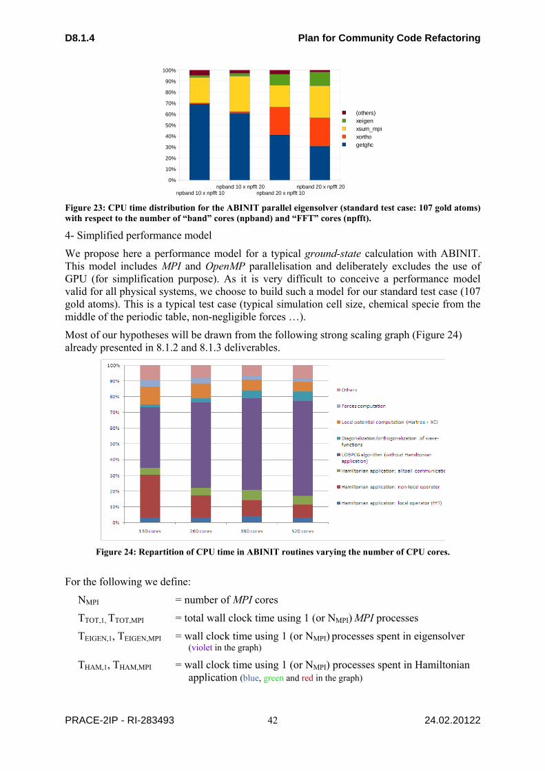
D8.1.4 Plan for Community Code Refactoring
PRACE-2IP - RI-283493 24.02.20122
42
Figure 23: CPU time distribution for the ABINIT parallel eigensolver (standard test case: 107 gold atoms) with respect to the number of “band” cores (npband) and “FFT” cores (npfft).
4- Simplified performance model
We propose here a performance model for a typical ground-state calculation with ABINIT. This model includes MPI and OpenMP parallelisation and deliberately excludes the use of GPU (for simplification purpose). As it is very difficult to conceive a performance model valid for all physical systems, we choose to build such a model for our standard test case (107 gold atoms). This is a typical test case (typical simulation cell size, chemical specie from the middle of the periodic table, non-negligible forces …).
Most of our hypotheses will be drawn from the following strong scaling graph (Figure 24) already presented in 8.1.2 and 8.1.3 deliverables.
Figure 24: Repartition of CPU time in ABINIT routines varying the number of CPU cores.
For the following we define:
NMPI = number of MPI cores
TTOT,1, TTOT,MPI = total wall clock time using 1 (or NMPI) MPI processes
TEIGEN,1, TEIGEN,MPI = wall clock time using 1 (or NMPI) processes spent in eigensolver (violet in the graph)
THAM,1, THAM,MPI = wall clock time using 1 (or NMPI) processes spent in Hamiltonian application (blue, green and red in the graph)
npband 10 x npfft 10 npband 10 x npfft 20
npband 20 x npfft 10 npband 20 x npfft 20
0%
10%
20%
30%
40%
50%
60%
70%
80%
90%
100%
(others) xeigen xsum_mpi xortho getghc

D8.1.4 Plan for Community Code Refactoring
PRACE-2IP - RI-283493 24.02.20122
43
TOTHER,1, TOTHER,MPI = wall clock time using 1 (or NMPI) processes spent in other routines (~15% of total CPU time, according to above graph)
SOMP,16 = OpenMP speedup of the kernel on 16 cores (~10)
SEIGEN-MPI = MPI speedup of the eigensolver on NMPI cores (0.8 NMPI)
SZEEV-MPI = MPI speedup of the ZEEV ScaLAPACK routine on NMPI cores
As previously mentioned we can estimate TZEEV-MPI≈20 if NMPI>20
Let us consider that we are running ABINIT over a number of MPI processes in the range ensuring a linear scaling of the Hamiltonian application (NMPI <500). Let us also consider that the sizes of matrixes are large enough to be above the ScaLAPACK activation threshold.
As shown by the previous graph we can estimate the total CPU time needed for a typical run:
TTOT,MPI ≈ TOTHER,MPI + TEIGEN,MPI + THAM,MPI ≈ (TEIGEN,MPI + THAM,MPI)/0.85
As assumed, the Hamiltonian application scales linearly:
THAM,MPI ≈ THAM,1 / NMPI
Meaning that:
TTOT,MPI ≈ TTOT,1/NMPI + (TEIGEN,MPI – TEIGEN,1/NMPI)/0.85
Now, for the eigensolver, let us divide the time in 3 parts (diagonalisation, orthogonalisation and communications) according to the Figure shown in the section 3-:
TEIGEN,MPI ≈ TDIAGO,MPI + (TORTHO,MPI + TCOMM,MPI)
The last two times are communications times.
For the diagonalisation, we can use ScaLAPACK (MPI) or a multithreaded (openMP) version of LAPACK. Assuming that the diagonalization is exclusively made by the processors of a single node, we can have (ScaLAPACK):
TDIAGO,MPI = TDIAGO,1/SZEEV-MPI/SEIGEN-MPI
Or (openMP):
TDIAGO,MPI = TDIAGO,1/SOMP,16/SEIGEN-MPI
For the communications, it is difficult to evaluate exactly what could be the performance improvement induced by the use of openMP. If we look carefully inside the LOBPCG algorithm we can roughly estimate the amount of communications as inversely proportional to the size of the eigenvalue problem in wave functions subspace. In other words, if the wave functions subspaces (blocks) are large they do not need to be orthogonalized to each other.
If we assume that the diagonalization step can be reduced by one or two order of magnitude using Scalapack or openMP, we can choose to diagonalize blocks of larger size (one single block of maximum size is possible) and thus make the communications disappear. In conclusion, a speed-up of diagonalization as described previously will probably suffice to significantly accelerate the code.
5- Validation procedure
The ABINIT package comes with a collection of automatic tests to verify the correctness of the results (~450 tests). ABINIT has to give exactly the same results according to the sensitivity (in terms of digits) defined for each test.

D8.1.4 Plan for Community Code Refactoring
PRACE-2IP - RI-283493 24.02.20122
44
Then the 107 gold atoms test (“standard” test) will be used to measure the performance improvement.
4.1.3 Plan for code refactoring: ground–state calculations using wavelets (BigDFT)
The main part of the plan is to improve the optimisation of BigDFT running it on one node. The idea is to build an automatic generation of code to test different strategies of optimisation for CPU first and then GPU.
BigDFT has more than 25 kernels to optimise and has no hot-spot operations. Optimising these kernels becomes problematic with the increasing numbers of new architectures. Another problem is that optimising a kernel on one core is not the right solution, because the main limitation is the bandwidth memory. We need to optimise kernels using all cores of one node or one socket.
1- Hybrid MPI/OpenMP test
The test is the ground-state calculation of a cluster made of 80 bore atoms done on CCRT-Titane (CCRT French centre, Intel processors) on one node (8 cores). There are 120 orbitals. This means that we can use 120 MPI processes as an upper limit. It is a rather small system. Figure 25 illustrates the efficiency and the speedup with respect to the number of MPI processes and threads. We can see that using 2 threads slightly changes the efficiency and is almost equivalent to using 2 times more MPI processes.
The different convolutions – which are the basic operations with wavelets functions – represent the main part of the calculation.
Figure 25: BigDFT on Titane-CCRT supercomputer: efficiency (solid blue curve) and speedup (dashed red line) with respect to the number of MPI processes and threads.
Now if we use a computer using AMD cores (CSCS-Palu, see Figure 26 below), then the results are different: the efficiency strongly decreases when all cores are used (24 cores). But we can use more threads (up to 4) with a small decrease of the efficiency.

D8.1.4 Plan for Community Code Refactoring
PRACE-2IP - RI-283493 24.02.20122
45
Figure 26: BigDFT on Palu-CSCS supercomputer: efficiency (solid blue curve) and speedup (dashed red line) with respect to the number of MPI processes and threads.
In Figure 27, we compare one node of both computers (24 AMD cores and and 8 Intel cores) using the best MI+threads configuration (i.e. only MPI processes).. We can see that 16 AMD cores are equivalent to 8 Intel cores.
Figure 27: Computer of time spent in convolutions on two different architectures (Titane-CCRT and Palu-CSCS)
2- Hybrid MPI/OpenMP and GPU test
If we combine OpenMP + MPI and GPU usage (OpenCL or CUDA) then we have different behaviours (see Figure 28). The main conclusion is that the use of GPU always gives a speedup (sometimes small). The best performances are obtained using OpenCL, CUBLAS for linear algebra and MPI processes. Comparing to CPU+mkl+MPI, we can have a speedup of 2 by adding only one GPU.
All these tests are very dependent on the considered system, namely the number of atoms and boundary conditions. It is possible to have a speedup of more than 10 when considering periodic boundary conditions with k points.

D8.1.4 Plan for Community Code Refactoring
PRACE-2IP - RI-283493 24.02.20122
46
In conclusion, it is really important to have optimised routines.
Figure 28: Speedup of BigDFT using GPUs
3- Automatic code generation
In order to simplify the maintenance of the optimised kernels, we tried to find a solution to automatically generate routines with different optimisation strategies: the number of unrolling loops, different patterns for the memory accesses, etc..
We have tested a first version based on the script language Ruby to generate different strategies of optimization. This is an elegant and easy to use language; our first results are promising. The main advantage is the ease to make changes and add new features. On this first example we prove the feasibility of the implementation.
In conclusion, the plan for BigDFT refactoring is to implement a complete solution of automatic code generation.
4.1.4 Plan for code refactoring: excited states calculations
The performance analysis done in [4] allowed us to identify the most critical parts of the code. On the basis of these results, we proposed four different modifications that should substantially improve the scalability of the GW code:
Implementation of a hybrid MPI-OpenMP approach Use of ScaLAPACK routines for the inversion of the dielectric matrix Implementation of a new MPI distribution scheme of the orbitals in order to
improve the load balancing during the computation of the exchange part of the self-energy
Use of MPI-IO routines to read the orbitals and the screening matrix from file
In order to assess the efficiency and the feasibility of these four different approaches, we have developed prototype codes that have been benchmarked using realistic parameters.
Subsequently we report the results of these tests, including an estimate of the parallel efficiency of the new implementation. Finally, a simplified performance model, whose parameters are estimated from the results of these preliminary tests, is presented and discussed.

D8.1.4 Plan for Community Code Refactoring
PRACE-2IP - RI-283493 24.02.20122
47
1- Hybrid OpenMP-MPI implementation
We have generalised the FFTW3 routines used in ABINIT so that the transforms can be executed in parallel with OpenMP (OMP) threads.
Figure 29 shows the parallel efficiency of the new implementation for different number of threads employed.
The benchmarks are performed using the FFTW3 interface provided by the MKL library.
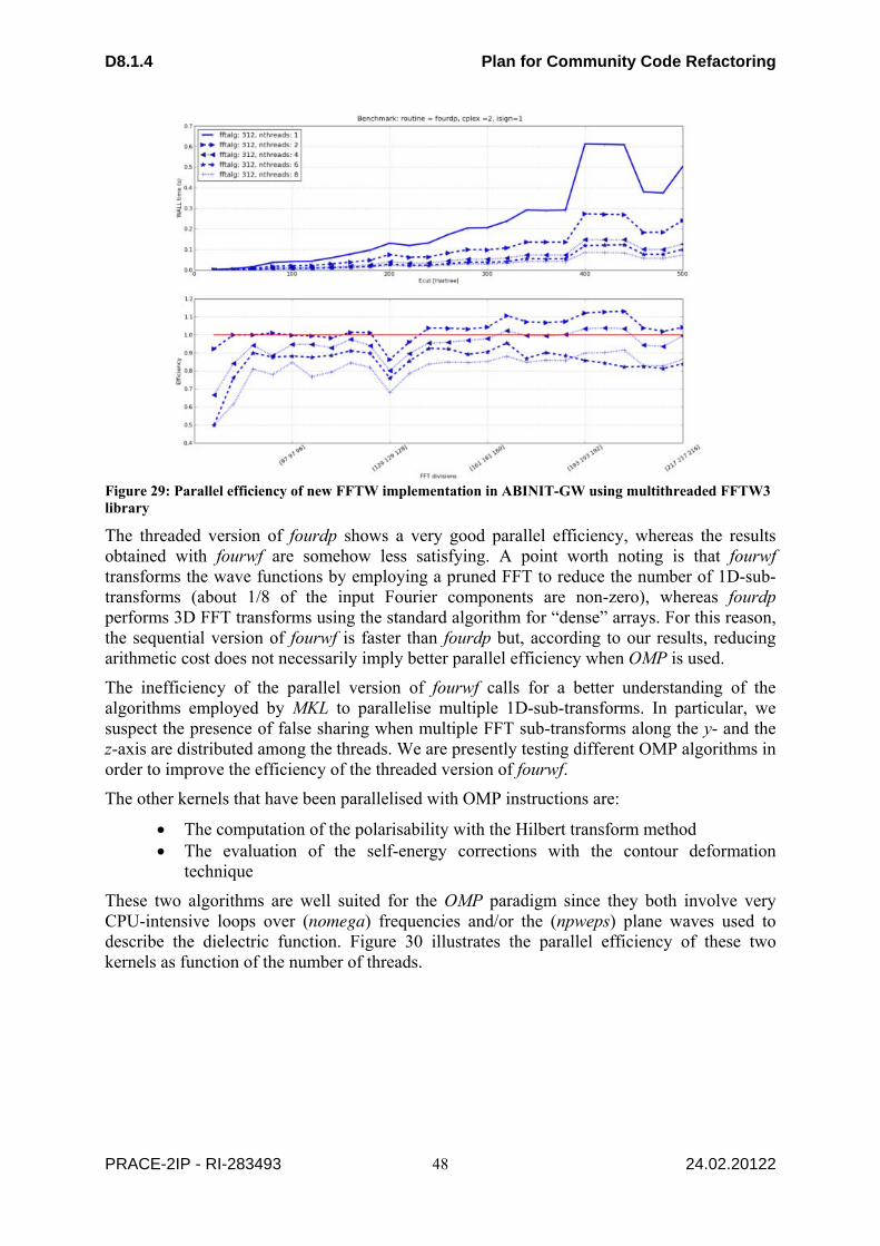
D8.1.4 Plan for Community Code Refactoring
PRACE-2IP - RI-283493 24.02.20122
48
Figure 29: Parallel efficiency of new FFTW implementation in ABINIT-GW using multithreaded FFTW3 library
The threaded version of fourdp shows a very good parallel efficiency, whereas the results obtained with fourwf are somehow less satisfying. A point worth noting is that fourwf transforms the wave functions by employing a pruned FFT to reduce the number of 1D-sub-transforms (about 1/8 of the input Fourier components are non-zero), whereas fourdp performs 3D FFT transforms using the standard algorithm for “dense” arrays. For this reason, the sequential version of fourwf is faster than fourdp but, according to our results, reducing arithmetic cost does not necessarily imply better parallel efficiency when OMP is used.
The inefficiency of the parallel version of fourwf calls for a better understanding of the algorithms employed by MKL to parallelise multiple 1D-sub-transforms. In particular, we suspect the presence of false sharing when multiple FFT sub-transforms along the y- and the z-axis are distributed among the threads. We are presently testing different OMP algorithms in order to improve the efficiency of the threaded version of fourwf.
The other kernels that have been parallelised with OMP instructions are:
The computation of the polarisability with the Hilbert transform method The evaluation of the self-energy corrections with the contour deformation
technique
These two algorithms are well suited for the OMP paradigm since they both involve very CPU-intensive loops over (nomega) frequencies and/or the (npweps) plane waves used to describe the dielectric function. Figure 30 illustrates the parallel efficiency of these two kernels as function of the number of threads.

D8.1.4 Plan for Community Code Refactoring
PRACE-2IP - RI-283493 24.02.20122
49
Figure 30: Parallel efficiency polarisability and self-energy kernels in ABINIT-GW using openMP
For these tests, we employed nomega=70 and npweps=531. Note that the parallel efficiency improves when larger values of npweps are used (not shown).
2- Computation of the inverse dielectric matrix with ScaLAPACK
The CPU time needed for the inversion of the dielectric matrix scales as npweps**3, hence this section of the code represents an important bottleneck in the case of systems with large unit cell. For this reason, a new kernel in which the inversion is done in parallel with ScaLAPACK routines has been implemented and benchmarked. Figure 31 shows the performance of the new implementation for different dimensions of the dielectric matrix.
Figure 31: Performance of the new implementation of the inversion of the dieletric matrix using ScaLAPACK
As already stressed in the ground-state section, the use of ScaLAPACK is beneficial only when the size of the matrix is larger than a threshold value that strongly depends on the architecture, the network, and the library used. Moreover, as shown in the figure, a brute force increase of the number of processors does not necessarily lead to faster computations. The forthcoming version of the GW code will accept a new input variable that specifies the

D8.1.4 Plan for Community Code Refactoring
PRACE-2IP - RI-283493 24.02.20122
50
maximum number of processors to use for the matrix inversion (see also the discussion in section 5 below).
3- New distribution of the orbitals
A new distribution scheme, in which all the occupied states are stored on each node, has been made available in ABINIT. This approach is more memory demanding than the standard algorithm, but it allows one to achieve an almost optimal distribution of the workload during the computation of the exchange part of the self-energy when the number of processors is larger than the number of occupied bands. Preliminary tests (not shown), performed on a relatively small number of processors (<32), confirmed the better scaling of the new implementation.
4- MPI-IO for the reading of the orbitals.
We have added the possibility of reading the orbitals and the screening function using collective MPI-IO routines. The new version has been tested on a relatively small number of processors. Additional tests are needed to assess the scalability of this part for large number of processors.
5- Validation procedure
In order to validate the new FFT kernels, we have written a small tool (fftprof) that tests the efficiency and the correctness of the different FFT libraries interfaced with ABINIT (FFTW3, MKL, Goedecker's library). The results produced by fftprof can be plotted with a Python script so that the user can select the optimal set of parameters (FFT library, number of threads, cache size) for a given FFT mesh.
The hybrid OpenMP-MPI implementation can be validated by running the standard GW tests available in the ABINIT test suite.
The parallel inversion can be validated with the new utility tool LAPACKPROF that runs selected ScaLAPACK routines for a given number of processors. lapackprof checks the correctness of the results and the efficiency of ScaLAPACK implementation so that one can find an optimal setup (number of processors, ScaLAPACK block size) for a given matrix size.
6-Simplified performance model
In what follows, we present a simplified performance model for a typical GW calculation based on norm-conserving pseudo-potentials and plane waves. The polarisability is evaluated for NOMEGA frequencies using the Hilbert transform method while the self-energy matrix elements are computed with the contour deformation technique.
This simplified model includes both the MPI and the OpenMP parallelisation. Most of our assumptions are derived from the strong scaling analysis presented in 8.1.2 [3] and 8.1.3 [4] deliverables, and from the results for the OpenMP version presented in the previous sections.
The total wall time of a sequential GW run (screening + sigma) is approximately given by:
T_TOT = T_FFT + T_GW + T_INV + T_OTHER
Where
T_TOT = total wall-clock time
T_FFT = wall-clock time spent in the FFT routines.
T_GW = wall-clock time spent in the GW kernels
T_INV = wall-clock time needed for inverting the dielectric matrix
T_OTHER = remaining portions of the code (MPI communications, IO, etcetera)
D8.1.4 Plan for Community Code Refactoring
PRACE-2IP - RI-283493 24.02.20122
51
To discuss the scaling of parallel implementation, we introduce the following quantities:
NMPI = number of MPI processes
NOMP = number of OMP cores
NOMEGA = number of frequencies in the screened interaction
We use T(NMPI,NOMP) to denote the total wall-clock time of the code executed with NMPI MPI processes and NOMP threads. According to this notation, the elapsed time of the sequential code will be indicated by T_TOT(1,1).
Since the orbitals are almost equally distributed among the MPI processes, we have:
T_FFT(NMPI,NOMP) = T_FFT(1,1) / (NMPI * σ_FFT_OMP(NOMP) )
Where σ_FFT_OMP(NOMP) is the OpenMP speedup of the FFT transforms with NOMP cores. According to our tests σ_FFTOMP(NOMP) ~ 0.9 NOMP when fourdp is employed.
The pure MPI implementation of the GW kernels scales as
T_GW(NMPI,1) = T_GW(1,1) / NMPI
The linear scaling (confirmed by the analysis performed in the precedent deliverables) is due to the fact that the number of calls to the GW kernels is proportional to the number of states that are almost equally distributed among the nodes. For the hybrid MPI-OpenMP implementation, one thus obtains:
T_GW(NMPI,NOMP) = T_GW(1,1)/( NMPI * σ_GWOMP(NOMP) )
Where σ_GWOMP(NOMP) is the OpenMP speedup of the GW kernels. Our preliminary results indicate that σ_GWOMP(NOMP) ranges between 0.7 NOMP and 0.9 NOMP when NOMP <= 4
The scalability of the algorithm that inverts the dielectric matrix strongly depends on the number of frequencies computed. In the previous implementation, the matrix inversion was distributed over frequencies and then performed in sequential. As a consequence, this section of the code was not scaling anymore when NMPI > NOMEGA. The new version based on ScaLAPACK routines presents a much better scaling given by
T_INV(NMPI) = T_INV(1,1)/(NOMEGA*σ_SLK(NSLK)) (NMPI > NOMEGA)
Where σ_SLK(NSLK) is the ScaLAPACK speedup with NSLK processors (the additional level of parallelisation due to OMP has been neglected, for the sake of simplicity). Our tests reveal that, for the typical size of the dielectric matrices used in our applications, σ_SLK(NSLK) ~ NSLK if NSLK < 8.
As stated, T_OTHER includes the wall-clock time spent in the MPI sections and in the IO routines. The previous tests shown that the GW code is not communication bounded (at least up to NMPI<512) and the introduction of the additional level of parallelism based on OMP will help reduce the number of communications. The use of MPI-IO routines should lead to better scaling of the IO sections with respect to the previous implementation based on Fortran IO, in particular when many processors are used.
4.1.5 Plan for code refactoring: linear response calculations
The linear-response part of the ABINIT code plays a specific, but important, role, allowing computing efficiently phonons, electric field responses, etc. However, due to lack of human time, it was not analysed in D8.1.2 [3] or D8.1.3 [4]. Appendix B to the present deliverable fills the gap. It provides a performance analysis, and presents four strategies for the improvement of linear response calculations.

D8.1.4 Plan for Community Code Refactoring
PRACE-2IP - RI-283493 24.02.20122
52
The performance analysis allowed us to identify the most critical parts of the code. For the test case (a barium titanate slab with 29 atoms), it was shown that the most time-consuming parts of the calculation have been parallelised efficiently over k-point and bands. These parts scale linearly, well beyond 256 cores. However, for a smaller number of cores, two bottlenecks appear: the first bottleneck is at the level of the initialisation of the ground state wave functions (reading from file, and spreading the data), the second is at the level of the routines that cannot be parallelised over k-point and bands, typically the treatment of density and potential. Moreover, the amount of memory that is needed for each processor scales as the number of bands times the number of plane waves, that is, quadratically with respect to the size of the system.
On the basis of these results, we propose in Appendix B four different modifications that should substantially improve the scalability of the linear response calculations:
Remove the IO-related initialisation bottleneck. In particular, use of MPI-IO routines to read the ground-state wave functions from file.
Parallelise several sections that cannot be parallelised over k-point and bands. These sections scale like the number of plane waves and/or the number of FFT points.
Distribute the ground state wave functions over the bands and/or the plane waves. Parallelise over the outer loop on perturbations.
We have made a first assessment of the efficiency and the feasibility of these four different approaches. This work has been started end of November 2011, and will be subject to further refinement. We base our assessment on the analysis of similar approaches implemented in other parts of ABINIT.
1- Remove the IO-related initialisation bottleneck
The initialisation is not satisfactorily parallelised over k-point, and does not take advantage of the band parallelisation. In the ground-state plane-wave part of ABINIT, the reading of wave functions has been parallelised using MPI-IO routines. It was observed that this wave function initialisation is very effective, such that the time needed is now negligible with respect to the other parts of the calculation. Although the reading and distribution is more complex in the case of the linear response calculation initialisation, we expect a similar behaviour for the ground-state plane-wave part of ABINIT.
2- Parallelise several sections that are performed sequentially
The operations done in the fourdp, vtorho3 and vtowfk3 do not have a workload that scales as the number of k-points times the number of bands. Of course, in the sequential mode of linear-response calculations, the associated time is completely negligible. However, as seen in the test, with more than 100 processors, they start to be important.
These sections scale as the number of plane waves (or the number of FFT grid points). They can be parallelised over these quantities. A similar parallelisation has already been done in the ground-state plane-wave as well as the excited state parts of ABINIT. They rely on OpenMP or MPI. With OpenMP, it will be possible, with little coding effort, to decrease the time by a factor of ten (as shown by unitary testing, see section 4.1.4). The MPI coding effort would be larger, but is not to be ruled out at this stage.
3- Distribute the ground state wave functions over the bands and/or the plane waves.
Although this task is not impacting the execution time, it will address an important limitation of linear response calculations for larger number of atoms. At present, all the processors treating the same k-point must store a copy of the wave functions for all states for that k-

D8.1.4 Plan for Community Code Refactoring
PRACE-2IP - RI-283493 24.02.20122
53
point. Thus, the memory requirement for one compute core increases with the size of the problem. One should distribute the ground-state wave functions among the processors, and treat the scalar product of ground-state and first-order wavefunctions accordingly. An OpenMP solution might be limited, so that MPI is to be preferred. The correct analysis of this strategy is to be refined, and actually this must be considered at the same time as the final choice of strategy for task 2 and perhaps even task 1. Again, a similar parallelisation has already been done in the ground-state plane-wave part of ABINIT, and proven effective.
4- Parallelise the outer loop on perturbations
When the bottlenecks addressed by tasks 1-3 will be removed, the possibility to parallelise over perturbations will be open. The number of perturbations can be quite large (on the order of 50 for our test case - however this test case is restricted at present to only one perturbation). The amount of communication is very small. The number of sequential parts with respect to this parallelisation is also very small. However, there is a load balancing problem, described in the appendix. For large systems, non-symmetric (the most time-consuming), more than one order of magnitude improvement of the execution time should be attainable.
5- Simplified performance model
Subsequently we sketch a simplified performance model for the test case presented in Appendix B. We rationalise the available data.
The total wall time of a sequential linear-response (LR) run is approximately given by:
T_TOT = T_INIT + T_WF + T_DENPOT + T_OTHER
Where
T_TOT = total wall-clock time
T_INIT = wall-clock time spent in the initialisation of the run
T_WF = wall-clock time spent in the operations done on the wave functions, after the initialisation
T_DENPOT = wall-clock time spent in the operations done on the density and potential, after the initialisation
T_OTHER = remaining portions of the code
To discuss the scaling of parallel implementation, we introduce the following quantities:
NP_KB = number of MPI processes on which the k-point and band load is distributed
NP_G = number of processes on which the plane waves / FFT load is distributed (could be OpenMP or MPI)
In the present test case, the communication time is negligible in most sections of the code, except in the initialisation section.
We use T_X(N_KB,N_G) (where X is TOT, INIT, WF or DENPOT), to denote the total wall-clock time of the code executed with NP_KG MPI processes and NP_G MPI processes or OMP threads. According to this notation, the elapsed time of the sequential parts of the code will be indicated by T_X(1,1).
In the present implementation, only the KB parallelisation is used, with:
T_INIT(NP_KB,1) = T_INIT(1,1)* f(NP_KB)
T_WF(NP_KB,1) = T_WF(1,1)/NP_KB
T_DENPOT(NP_KB,1) = T_DENPOT(1,1)

D8.1.4 Plan for Community Code Refactoring
PRACE-2IP - RI-283493 24.02.20122
54
T_OTHER(NP_KB,1) = T_OTHER(1,1)
The time T_WF(1,1) being a very large fraction (more than 99%) of the total time T_TOT(1,1), the speed up can reach about 80 on the test case.
The detrimental factor f(NP_KB) is larger than 1. It is actually close to 1 for a small number of processes NP_KB, until NP_KB increases beyond about 64. The presence of this factor has the aim to indicate roughly the behaviour of the initialisation times, whose scaling is not well characterized at present.
Following strategy 1, that is, using MPI-IO to initialize the wave functions, one expect to get rid of the bad scaling behaviour of the communications. The initialisation time can be predicted to change to
T_INIT(NP_KB,1) = T_INIT(1,1)/NP_KB
(without the presence of a detrimental factor f(NP_KB)).
Following strategy 2, the T_DENPOT time can be predicted to change to
T_DENPOT(NP_KB, NP_G) = T_DENPOT(1,1)/ σ_G(NP_G)
Where σ_G(NP_G) is the efficiency of use of the NP_G cores to speed-up the density and potential sections of the code. Note that most of the operations on the density and potentials sections of the code are done in sections in which the wave functions are not present. Thus, without increasing the number of cores, a speed-up of these parts can be realized. In case of OpenMP, taking the unitary tests done for the excited state calculations (see section 4.1.4), one can expect a fair speed up, up to 6 or 8, without problem. MPI coding will allow more speed-up, but at the expense of a more difficult coding. Still, this would also solve the distribution of array problem.
Explicitly, supposing a maximum number of cores NP, the execution time should be
T_TOT(NP,NP) = T_INIT(1,1)/NP +
T_WF(1,1)/NP +
T_DENPOT(1,1)/ σ_G(NP) +
T_OTHER(1,1)
The first goal of strategy 3 is not to decrease the execution time, but to allow to use more efficiently the memory. Still, this might impact the scaling of different sections of the code.
Finally, the strategy 4 addresses a larger demand, for which the test case is to be modified, by using more than one perturbation. Introducing the number of perturbations N_PERT, the time of a run with N_PERT, compared to the time for only 1 perturbation, will be
T_TOT(NPERT) = T_INIT + N_PERT*(T_WF + T_DENPOT + T_OTHER)
This level of perturbation will allow to use a maximal number of NP_PERT * NP processes. The load balancing of this level of parallelisation is to be addressed, though.
6- Validation procedure
In addition to the test case that has been used to make the performance analysis for PRACE-2IP, there is (a) another test case presented in the ABINIT tutorial on the parallelisation of the linear response section of ABINIT, (b) numerous non-regression tests for the linear response case present in the ABINIT automatic test suite (about 100), and (c) even more non-

D8.1.4 Plan for Community Code Refactoring
PRACE-2IP - RI-283493 24.02.20122
55
regression tests for the other aspects of ABINIT. So, as soon as the modifications of the code are committed to the ABINIT worldwide repository, they will be tested and validated.
4.2 Quantum ESPRESSO
4.2.1 Introduction
Quantum ESPRESSO is an integrated suite of computer codes based on density-functional theory, plane waves, and pseudo-potentials. The acronym ESPRESSO stands for opEn Source Package for Research in Electronic Structure, Simulation, and Optimisation.
Two are the main goals of the project: 1) to enable state-of-the-art materials simulations, and 2) to foster methodological innovation in the field of electronic structure and simulations by providing and integrating highly efficient, robust, and user-friendly open source packages containing most recent developments in the field.
The Quantum ESPRESSO distribution offers users a highly portable and uniform installation environment. The web interface, qe-forge, provides to potential developers an integrated development environment, which blurs the line separating development and production codes and engages and nurtures developers by encouraging their software contributions.
Quantum ESPRESSO is freely available under the terms of the GNU General Public License (GPL).
4.2.2 Target a general refactoring of the suite
Quantum ESPRESSO is actually structured as a suite of many packages, each of them is devoted to a particular kind of calculation. The basic are the two DFT engines, PWscf (plane-wave DFT self-consistency calculations) and CP (Car-Parrinello molecular dynamics). Inside the suite different levels of dependencies exist. For instance, some packages such as PHonon, TDDFPT or GIPAW are linked to the same computational kernels used by PWscf and CP, while others, such as PLUMED or YAMBO not.
The overall structure is already organised to take advantage of Fortran 90 modularisation features, and developers already took care of avoiding the replication of similar portions of code in different parts of the suite. Nonetheless, a recent developers meeting1 with representative computational scientists from CINECA and ICHEC came to the conclusion that it is still necessary to work on this direction to functionally refactoring the deepest part of the distribution.
A refactorisation work should be performed in order to rewrite some of the most used subroutines, belonging to the DFT engine PWscf and the linear response package PHonon, as low level libraries. The creation of such libraries would give a higher level of modularity that could help to maintain most of the packages and to sustain further developments.
A particular case of refactoring needs is the proper implementation of hybrid functionals. The use of Hybrid functionals, i.e., inclusion of a portion of exact-exchange (EXX) inside traditional functionals, is nowadays the better compromise between physical meaning and computational cost. The user community is, indeed, strongly pushing in this direction. At this moment, the possibility of adding an exact-exchange fraction is already present in some packages, PWscf and CP, for some specific calculations. However, it is absolutely necessary to re-engineer and extend it, as many of the advanced features are only available with traditional functionals.
1 Quantum Espresso developers workshop, Trieste, 24 January 2012

D8.1.4 Plan for Community Code Refactoring
PRACE-2IP - RI-283493 24.02.20122
56
4.2.3 OpenMP enhancement
The new developments of computer architectures are mainly towards systems that either contain many-cores and/or are accelerated. In both cases, for ab-initio codes a simple parallelism based on MPI is no longer sufficient. Many community codes still implement parallelisation strategies that were implicitly imposed by the previous generation of HPC architectures.
The basic parts of the Quantum ESPRESSO suite, PWscf and CP, have already been parallelised on many levels, including a low-level parallelisation using OpenMP. The performance modelling on both PWscf and CP has shown that a multi-thread approach allows almost linear scaling over the number of threads (4 or 6). According to the needs of the material science community, it is very important to extend this level of parallelisation even to those parts of the distribution where it is not yet used. Good candidates are the linear response package PHonon and the stresses/forces calculations in PWscf. A global inspection of the distribution might be useful to discover specific non-optimised routines that certain scientific cases may trigger.
A refactorisation of the kernel packages aimed at further incorporating OpenMP to other relevant codes will permit the codes to run on upcoming new architectures by better exploiting the available memory. This, in turn, will make possible to run simulations of extended systems without big loss of efficiency. Focusing on the PRACE ecosystem, a particular case where the multi-threading approach becomes crucial is the new Blue Gene/Q architecture. In this case, compute nodes are built out of a single 4-way SMT CPU with 16 compute cores sharing 16 GByte RAM. Moreover, using more than one thread on each core makes it possible to exploit the capabilities of all FPU units embedded in each die. This obviously reflects the need to run jobs in a hybrid mode, using well-know mixed parallelism strategies (coupling MPI for inter-node communications and OpenMP for intra-node parallelism).
4.2.4 Parallelism over bands
A further possible improvement that involves the high-level parallelism already in place in two portions of PWscf and GIPAW is the addition of a new parallelisation level over bands.
This can be implemented by splitting loops that looks like:
do i = 1, nbands
… (independent operations over the i index)
end do
in a way that groups of bands are processed independently and only at the end reduction or collect operations are performed. These new synchronisation points could introduce costs, but in the end a relevant increase in scalability of the overall calculation might be obtained.
Within PRACE-1IP project, inside the WP 7.2, an exploratory work has been performed on two computational-intensive EXX routines: vexx and exxen2. Linear scalability has been obtained with a high parallel efficiency. Up to now, data structures were replicated across the new level of parallelism. In order to decrease the memory footprint of the calculation, a full distribution of the data is now needed.
4.2.5 Improve common computational kernels: linear algebra and Fast Fourier Transforms
Linear algebra (matrix-matrix multiplications and eigen-solvers) and Fast Fourier Transforms represent a set of basic dominant operations across most of the packages of the suite. In PWscf, varying with the scientific case, matrix-matrix operations consume up to 40% of the

D8.1.4 Plan for Community Code Refactoring
PRACE-2IP - RI-283493 24.02.20122
57
overall wall-time. In the CP package, computation is usually dominated by distributed 3D-FFT transformations.
Linear algebra operations and FFT transformations now rely on external libraries. LAPACK and BLAS represent standard de-facto and CPU vendors usually provide their own implementation that targets their specific hardware (i.e. Intel MKL, AMD ACML, IBM ESSL, CRAY libSCI and others).
In addition to these libraries, several new open-source projects exist. PLASMA, developed by the Innovative Computing Laboratory (ICL) at the University of Tennessee, addresses the critical and highly disruptive situation engendered by the introduction of multi-core architectures. As first step, investigating where and how to plug the PLASMA library inside most of the Quantum ESPRESSO packages might help to assess (and then improve) the efficiency of the multi-threading.
On the other hand, the same research group develops and maintains another package called MAGMA. The MAGMA project aims to develop a dense linear algebra library similar to LAPACK but for heterogeneous/hybrid architectures, starting with current "Multi-core+GPU" systems. MAGMA has been already used to accelerate the serial eigensolvers used by PWscf to solve for the specified number of states using iterative (Davidson) diagonalisation. Diagonalisation can be very expensive in a parallel computation if a serial approach is used. For this reasons recently a parallel algorithm based on ScaLAPACK has been introduced. The measured scalability of this approach is good, but it cannot be increased too much (especially if the future scenario is to run simulations over thousands of cores distributed across hundreds of nodes). This potential bottleneck can be resolved by keeping a low number of MPI processes and accelerated local computations. This can be achieved by re-writing the diagonalisation routines or by a distributed version of MAGMA (D-MAGMA is currently under development). Both strategies should be pursued to keep a level of freedom and independence from third-party high-specialised libraries.
Speaking about the FFT, the activity undertaken to accelerate it with GPUs has already produced some benefits. Gathering and redistributing all the distributed data in such a way to perform the computation locally is a winning strategy, because, unlike in linear algebra where the amount of computation is usually O(n3), the computational cost of the FFT is usually O(n log n). Both CPU and GPU performance benefits from this approach. Further step aims to optimise the code as much as possible by implementing a reliable and portable mixed parallelism that couple MPI and OpenMP or MPI and GPU code.
4.2.6 Outlook to OpenACC
Within PRACE-1IP WP 7.5 the acceleration of PWscf has been completed. The accelerated code targets NVIDIA GPGPU using both explicit CUDA kernels and CUDA-enabled libraries.
Performance analysis underlined that the self-consistency loop (see Fig.13, Deliverable 8.1.3 [4]) is usually computationally more expensive than the calculation of stresses, forces and new atomic positions. Since real scientific simulations perform the high-level structure optimisation loop many times, the stresses and forces calculations become relevant. In the case of the CP code, the situation is even worse. In fact, the computation of stresses almost doubles the computational cost of each time step. Accelerating the computation of these contributions using GPUs will have a significant impact to on the overall performance.
Due to the complexity of the code, a large amount of effort may be required to port those kernels with CUDA. The new direct-based paradigm OpenACC will allow programmers to create high-level host+accelerator programs by defining specific “regions” that can be off-
D8.1.4 Plan for Community Code Refactoring
PRACE-2IP - RI-283493 24.02.20122
58
loaded to the accelerator. The use of OpenACC has several potential advantages: removing the need to explicitly initialise the accelerator, managing transparently data transfers between the host and accelerator, portability across several compilers and environment, and, last but not least, the automatic recognition and utilisation of other types of accelerators in the future.
It is reasonable that a first exploration and evaluation phase can be performed using a direct-based paradigm consistent with the OpenACC standard. Moreover, the gradual adoption of OpenACC will push the developers’ community to work on the current code to make it more OpenMP-friendly. As soon as more compilers will support OpenACC, the transition to the new paradigm will be smooth. This activity will perfectly couple the improvement of the multi-threading capabilities at CPU side.
4.2.7 Conclusions
The work of refactoring on the Quantum ESPRESSO suite could be summarised in the following actions:
1) improvement of the linear algebra part, taking into account the development oriented to new architectures such as GPUs and, more generally, accelerators;
2) OpenMP extension and parallelism on bands on other parts of the distribution where it is not yet implemented;
3) general and deep refactoring with special regards to modularisation techniques, obtained by removing any redundant portions of code.
The first one of these actions is aimed at obtaining a measurable improvement in the performance of the computational kernels. These kernels, once the work described in action 3 will be accomplished, would be linkable to any of the dependent packages of the Quantum ESPRESSO distribution.
The second of the above-mentioned actions will permit the enlargement of physical systems to study, by removing the limiting constraint on RAM memory. In particular, this improvement will benefit the usage of particular kinds of architecture where a hybrid MPI+OpenMP approach is more desirable. This action is really mission-critical, if the current roadmap to reach deployed exa-scale systems with hundreds of thousands of cores will continue as expected.
The third action is probably the most radical one. If a modularisation of the DFT engine PWscf and the linear response package PHonon is successfully achieved, this will change and improve of the numerical algorithms in the near future. Modularisation helps the process of including into the public code new developments by research groups that are not core developers. An example in this sense is the implementation of hybrid functionals, which is strongly pushed by the user community since it allows more realistic simulations of large systems of interest.
The Quantum ESPRESSO distribution includes a wide sample of short examples that are intended for testing of the codes. Such examples will be a useful tool to validate the above-mentioned improvements that will be made to the code. Furthermore, the test cases showed in the D8.3.2 and D8.3.3 will remain the baseline to establish how code performance changes during the work of refactoring.
4.2.8 Work plan
The work on Quantum ESPRESSO will involve CINECA, ICHEC and DEMOCRITOS. The work on the three above described macro-areas is almost independent and can be, using versioning tools such as SVN, performed in parallel.

D8.1.4 Plan for Community Code Refactoring
PRACE-2IP - RI-283493 24.02.20122
59
The effort will be shared, between CINECA, ICHEC, CSCS and the DEMOCRITOS community.
Releases of the codes will be made available after successful testing. We set two milestones:
MS 1: January 2013 presentation of the work performed and report at the Quantum ESPRESSO developers workshop
MS 2: October 2013 release of a version implementing the improvements described above.
4.3 Yambo
Yambo [33] is an ab initio code for calculating quasiparticle energies and optical properties of electronic systems within the framework of many-body perturbation theory (MBPT) and time-dependent density functional theory (TDDFT). Quasiparticle energies are calculated within the GW approximation for the self-energy. Optical properties are evaluated either by solving the Bethe–Salpeter equation or by using the adiabatic local density approximation.
The main performance problem of Yambo resides in the inversion of the response function, for which ScaLAPACK seems not to bring any scaling improvements. We will start by analysing the developers’ implementation of ScaLAPACK and fine-tuning it. Following this, we propose MAGMA for the LU factorisation and also to replace LU-factorisation based Gaussian elimination by Gauss-Jordan elimination. If the problem is solved earlier than expected, we propose to improve the code further by implementing ELPA as eigensolver for the Bethe-Salpeter equation.
We expect to devote 6 months to this task, according to the following timeline:
Figure 32: GANTT chart for Yambo
The validation of the modifications will be done using the input files in the current tutorial of the program. They are already being used by the developers for this purpose.
4.4 Siesta
SIESTA (Spanish Initiative for Electronic Simulations with Thousands of Atoms) is both a method and its computer program implementation, to perform electronic structure calculations and ab initio molecular dynamics simulations of molecules and solids.
The analysis presented in deliverables D8.1.2 [3] and D8.1.3 [4] pointed out that the most costly code section is the diagonalisation, so that the best approach for increasing the parallel performance is finding a better scaling method for solving the generalised eigenvalue problem than the currently used ScaLAPACK library.
March 2012 May 2012 July 2012 September 2012 November 2012 January 2013 March 2013
Implementation of a LU factorization based on MAGMA
May 1, 2012 – Jul 31, 2012
Benchmarking, validating and fine-tuning of the Gauss-Jordan implementation
Nov 1, 2012 – Jan 31, 2013
ScaLAPACK benchmarking, validating and fine-tuning
Feb 1, 2012 – Jun 30, 2012
Replacement of LU-factorization based Gaussian elimination by Gauss-Jordan elimination
Sep 1, 2012 – Nov 30, 2012
Benchmarking, validating and fine-tuning of the MAGMA implementation
Jul 1, 2012 – Oct 31, 2012

D8.1.4 Plan for Community Code Refactoring
PRACE-2IP - RI-283493 24.02.20122
60
The Sakurai-Sugiura (SS) method has the potential for using many processors efficiently, because it offers a multilevel parallelisation in a very natural way. Furthermore one can exploit the sparsity of the matrices to diagonalise.
To provide better performance also for small platforms, it would also be valuable to examine the potential of recent developments in the field of eigenvalue solvers on GPUs.
4.4.1 Sakurai-Sugiura Algorithm
This method is meant to find eigenpairs in a given domain of the spectrum. The number of eigenvalues that can be found is limited, depending on some parameters of the algorithm. If a big fraction of the spectrum has to be calculated, the range of interest has to be divided into subdomains.
From a computational point of view the algorithm consists of the following basic steps (for each subdomain):
1. Constructing and solving a set of complex-valued linear equations of the original matrix size, each with multiple right hand sides.
2. Summing up the solutions of the systems for getting a transformation matrix Q.
3. Projecting the original matrices H and S to a smaller subspace by matrix-multiplications QTHQ and QTSQ
4. Finding the eigenpairs of the smaller system and doing a back-transformation of the results.
5. Selecting the correct eigenpairs from the results
The first step is supposed to be the most costly since many linear systems of the original size have to be solved. So basically the SS algorithm shifts the problem of finding eigenpairs to solving linear systems, which is much easier to handle. So the total performance depends on the linear solver used and the efficiency of the parallelisation.
Parallelisation can be implemented at three different levels:
1. The most coarse-grained level is the division into subdomains. They are totally independent of each other, so there is no communication overhead. The total running time will be given by the most expensive domain. The efficiency depends on the load balance, but since all costly operations do not depend on the domain, the load balancing is expected to be good.
2. In each subdomain, the linear systems can be solved in parallel. Also this parallelisation does not need any communication, but when solving systems consecutively some data can be reused. Due to the similarity of the linear systems a very good load balancing is expected.
3. Also a parallel linear solver can be implemented. This might be useful, since only on this level can the original matrix be split for saving memory on one process.

D8.1.4 Plan for Community Code Refactoring
PRACE-2IP - RI-283493 24.02.20122
61
Figure 33: Visualisation of the outer two levels of parallelisation. The first level is the division of the domain. The first step in each domain is solving the linear systems, which can be done in parallel. Afterwards all processors can be used for doing the following computations in parallel.
While for the first two levels an MPI parallelisation is preferable, one might use different technologies for the linear solver. One possibility would be using one node with a multithreaded linear solver. Another idea is to use a GPU-based solver. Since many of the following operations are matrix-matrix and matrix-vector multiplications, GPUs might be used efficiently also for these tasks. This offers an opportunity to use many GPUs in parallel.
The computational effort depends strongly on some internal parameters of the algorithm. Those, in turn, are related to the desired accuracy on one hand, and on the other hand also on the available information about the spectrum. Since the diagonalisation is done in an iterative loop, information from previous iterations can be reused.
Work plan:
The work plan for this part accounts for the following steps.
1. Developing a prototype for examining the potential of the method and for finding an efficient sparse linear solver (a detailed work plan for this part is given in figure Figure 34. Milestones are:
M 8: Showing functionality and stability of method
M 14: Deciding on linear solver to implement
M 17: Significant performance data before going to final parallelization and implementation
2. Implementing the new eigensolver into Siesta and examining data-reuse and parameterisation, to try to obtain a "black-box" method that works automatically.
3. Final optimisation
This can be done for several linear solvers based on different technologies.
Figure 34: GANTT chart for the work on SS algorithm.

D8.1.4 Plan for Community Code Refactoring
PRACE-2IP - RI-283493 24.02.20122
62
4.4.2 Using GPU-based eigenvalue solver
Due to the efficient basis set of Siesta, many physically interesting problems can be computed on a single workstation. Thus reducing the computation time by implementing the newest GPU-based eigensolvers (e.g., the MAGMA library) can be interesting for many users.
Work plan:
1. Exchanging ScaLAPACK by MAGMA in serial mode.
2. Implementing the using of all cores of a hybrid (CPU/GPU) node or workstation.
4.4.3 Testing and Validation procedure
The Siesta distribution has a whole directory of feature-related tests that can be run automatically. These tests are typically small, so they are useful for correctness testing but not for performance testing.
The test examples water_pt, DNA, and Hemoglobina, presented in deliverables D8.1.2 [3] and D8.1.3 [4], represent systems with different features and sizes, and will thus be used for analysing performance and also correctness for larger systems.
4.5 Octopus
Octopus is an implementation of Time-Dependent Density Functional Theory (TDDFT) on a real-space grid. Octopus performs real-time propagation of the TDDFT equations in order to simulate the dynamics of electrons and nuclei under the influence of external time-dependent fields.
There are two main run modes in Octopus: ground-state calculations and time-propagation. The former is a pre-requisite of the latter, which is the main run mode of Octopus. There are two main performance problems to be tackled, one in each run mode.
For ground-state calculations, we will address the problems of the LOBPCG eigensolver when running parallel in states. An implementation within ScaLAPACK was already started by the code developers, but it is still very crude and was neither benchmarked nor fine-tuned. We plan to finish this implementation and refine it according to the results of benchmarks. If the performance gain is insufficient, we will try to develop a very thin reimplementation of BLACS on top of MPI with topologies (BLACS assumes a 2D topology), in order to allow for the use of a subset of the processors in ScaLAPACK.
For the time-propagation runs, the main bottleneck is the Poisson solver, as, in this run mode, the main physical operation is just the propagation in time of the Kohn-Sham wavefunctions computed in a previous ground-state run. At each time step, this propagation amounts to a multiplication of each wavefunction by the Hamiltonian matrix, followed by the re-computing of the Hamiltonian. Parallelisation in real-space domains and wavefunctions is trivial except for the “Hamiltonian recomputing” part. And in that part, the Poisson solver is the main bottleneck. The developers are already working on this problem and the proposed solution is to implement a parallel FFT (PFFT) Poisson solver and to also code an implementation of the fast multipole method (FMM). PFFT would be used for medium-size runs and FMM for very large runs. We plan to work on the grid re-partitioning that occurs after each call to PFFT. This is a communication-intensive step that can degrade the performance to the point of rending PFFT impracticable. We will also collaborate with the developers on testing and improving both implementations.
We expect to devote 6 Ms to these tasks, according to the chart in Figure 35.

D8.1.4 Plan for Community Code Refactoring
PRACE-2IP - RI-283493 24.02.20122
63
Figure 35: GANTT chart for Octopus.
In order to validate and benchmark the code modifications we will use the testing procedure already implemented by the developers of the code. This consists of a testsuite currently encompassing 300 different runs. We will only use the testsuite runs directly affected by the modifications. The benchmarking will be done using the runs included in PABS, as Octopus is part of it.
4.6 Exciting/ELK
4.6.1 Overview
Exciting
A full-potential all-electron density-functional-theory (DFT) package based on the linearized augmented plane-wave (LAPW) method. It can be applied to all kinds of materials, irrespective of the atomic species involved, and also allows for the investigation of the atomic-core region. The code particularly focuses on excited state properties, within the framework of time-dependent DFT (TDDFT) as well as within many-body perturbation theory (MBPT). The code is freely available under the GNU General Public License.
Elk
An all-electron full-potential linearized augmented-plane wave (FP-LAPW) code with many advanced features. Written originally at Karl-Franzens-Universität Graz as a milestone of the EXCITING EU Research and Training Network, the code is designed to be as simple as possible so that new developments in the field of density functional theory (DFT) can be added quickly and reliably. The code focuses on ground state properties with some effort devoted to excited state properties. The code is freely available under the GNU General Public License.
Both Exciting and Elk codes are successors of the original EXCITING FP-LAPW code and thus bear a lot of common algorithms and functionality. Both codes have a major bottleneck of poor scalability with respect to a number of atoms in the unit cell. Thus the “Performance analysis” [3] and “Code improvement” [4] phases are aimed at identification and elimination of this bottleneck and the goal of the code refactoring is set to create a fast and scalable ground-state LAPW solver.
4.6.2 Plan for code refactoring
The analysis of Exciting/Elk codes shows that the straightforward optimizations of the existing implementations would not be efficient without a fundamental change of the wave-functions representation. The proposed representation is based on the explicit knowledge of the radial basis functions for each azimuthal quantum number and is already implicitly used in some parts of the Exciting code. The change of the wave-function representation will impact the following major parts of the code: construction of the first- and second-variational wave
March 2012 May 2012 July 2012 September 2012 November 2012 January 2013
(Re)implementation of PFFT
Feb 1, 2012 – Mar 31, 2012
Benchmarking, validating and fine-tuning of the PFFT implementation
Apr 1, 2012 – Jun 30, 2012
Benchmarking, validating and fine-tuning of the FMM implementation
Aug 1, 2012 – Oct 31, 2012
ScaLAPACK benchmarking, validating and fine-tuning
Apr 1, 2012 – Aug 31, 2012
BLACS reimplemenation
Sep 1, 2012 – Jan 31, 2013

D8.1.4 Plan for Community Code Refactoring
PRACE-2IP - RI-283493 24.02.20122
64
functions, setup of the charge density and magnetization, calculation of matrix elements of any operator in the basis of first- or second-variational states (including setup of the second-variational Hamiltonian). The analysis also reveals a lot of functionality that should be common to all LAPW-based codes.
Thus, the following objectives are set:
1. Isolate generic algorithms of the linearized augmented plane-wave (LAPW) method into a separate reusable library, independent of a particular LAPW code implementation. This effort has a purpose of splitting code development into a “physics” part (maintained by a particular LAPW code community) and a common backbone (maintained by advanced code developers).
2. Design new scalable LAPW library with the capability of handling large unit cells with hundreds of atoms and running on hundreds to thousands of nodes on modern hybrid/multicore systems. The maximum number of atoms that the library can run should depend on the capabilities of the underlying generalized eigenvalue solvers only.
3. At the same time the experience of other community codes (for example ABINIT) could be used to set up an automated test suite for a constant check of code revisions. A lot of attention has to be paid to various compilation and runtime possibilities (MPI single threaded, MPI+OpenMP, MPI+OpenMP+GPU) on several platforms. Thus the support of a computing center providing the hardware for such a test-farm is needed. Also, “canonical” tests (for example, equilibrium lattice constants obtained in LDA) should be set up for the purpose of testing the “physics” part of the code.
The following steps are proposed to achieve the required objectives:
4. Create a prototype LAPW library. At this stage a new wave-function representation will be adopted, which will serve as a foundation for further algorithmic optimizations.
5. Together with (1): introduce changes to the Exciting code to work with the prototype library. Make initial crosschecks and validations.
6. Guarantee that the basic Exciting functionality (L(S)DA+(U)+(SO) ground-state calculations, collinear and non-collinear magnetic configurations, structure relaxation and forces) are reproduced. At this stage it should be possible to compute unit cells with ~100-200 atoms. Perform a structure optimization test run for a system with ~100 atoms.
7. Make use of parallel, generalized eigenvalue solvers based on different technologies (shared memory systems, GPUs). This will be a qualitative step towards “103 atoms” calculation.
8. Parallelize the other parts of the library, with particular respect to data distribution and generation, which is closely related on the selected eigenvalue solver(s).
9. Switch to high-performance I/O libraries such as HDF5 for the purpose of fast reading and writing of large data structures (for example, eigen-vectors or eigen wave-functions).
10. Complete with the ground-state optimizations and debugging of the LAPW library.

D8.1.4 Plan for Community Code Refactoring
PRACE-2IP - RI-283493 24.02.20122
65
The following last two items will be part of the phase after M19-24.
1. Show that the new library can be linked (after some inevitable modifications) to other LAPW codes, such as Elk. This will prove that at least two of the available LAPW codes can benefit from the proposed development model.
2. Check if excited states branch of the Exciting code can also be incorporated into the LPAW library.
4.6.3 Performance and scaling analysis of the core algorithms
The following notation is adopted:
N – number of atoms in the unit cell
NMPI – total number of MPI ranks
NMPI-k – number of MPI ranks for a given k-point
Nthread – number of threads (or cores) per MPI rank
T(..) – time for a task in brackets
O(..) – algorithm or data complexity
At each iteration of the ground state calculation the following steps are performed:
Step complexity time to solution notes
setup radial integrals
O(N) T(O(N)) / (min(N, NMPI) * Nthread)
involves MPI reduction of arrays with O(N) size
setup first-variational Hamiltonian and overlap matrices
O(N3) T(O(N3)) / (NMPI-k * Nthread)
possible candidate for a GPU implementation
diagonalize first variational secular equation
O(N3) T(O(N3)) / NMPI-k
depends strongly on particular implementation of a parallel eigen-value solver
setup first-variational wave-functions
O(N3) T(O(N3)) / (NMPI-k * Nthread) involves MPI reduction of arrays with O(N2) size across NMPI-k nodes
setup second-variational Hamiltonian
O(N3) T(O(N3)) / (NMPI-k * Nthread)
second variational matrix is small and not considered for MPI parallelization; involves MPI reduction of matrix with O(N2) size across NMPI-k nodes
diagonalize second-variational Hamiltonian
O(N3) T(O(N3)) / Nthread
because the matrix size is small the threaded LAPACK or GPU implementation is considered for

D8.1.4 Plan for Community Code Refactoring
PRACE-2IP - RI-283493 24.02.20122
66
Step complexity time to solution notes
diagonalization; involves MPI broadcast of matrix with O(N2) size across NMPI-k nodes
setup second-variational wave-functions
O(N3) T(O(N3)) / (NMPI-k * Nthread)
setup charge density and magnetization
O(N2) T(O(N2)) / (NMPI * Nthread)
includes MPI reduction of density matrix with O(N) size across all NMPI nodes
setup Hartree potential
O(N2) T(O(N2)) / (NMPI * Nthread)
includes MPI reduction of Hartree potential with O(N) size across all NMPI nodes
setup exchange-correlation potential
O(N) T(O(N)) / (min(N, NMPI) * Nthread)
includes MPI reduction of XC potential with O(N) size across all NMPI nodes
4.6.4 Work plan
The objectives identified above will be pursued by ETH according to the timeline presented in Figure 36.
Figure 36: GANTT chart for Exciting/ELK

D8.1.4 Plan for Community Code Refactoring
PRACE-2IP - RI-283493 24.02.20122
67
5 Particle Physics
Lattice QCD is a computationally demanding approach for studying the theory of the strong nuclear force known as Quantum Chromo Dynamics. QCD is believed to be the fundamental theory of the strong interaction which describes the interaction between quarks and gluons. Because of the large coupling at low energies, analytical computations using perturbation theory is not possible. The goal of lattice QCD is to make ab-initio calculations in QCD and compute physical observables such as the Hadron spectrum starting from this fundamental theory. In this approach, the space-time continuum is replaced by a discrete hyper-cubic volume with periodic boundary conditions, i.e., a 4-dimensional torus. Quark fields are described by what is called a spinor field ψ(x) at each lattice site x while gauge fields are described by what is called links U(x,ν) for each site x and direction ν. A spinor ψ(x) is a 12 component complex vector arranged as 4 structures (for 4 spin components) each is a 3 component complex vector (for 3 colours). The gauge (gluon) links U(x,ν) is 3 by 3 complex unitary matrix which is a member of the SU(3) gauge group. U(x,ν) connects spinor fields at sites x and where a is the lattice spacing and is a unit vector in the direction. In Figure Figure 37 a schematic representation of the lattice setup is shown.
Figure 37: A schematic presentation of the Lattice setup in 2 dimensions
In this deliverable, we summarise our performance study results for the prototype lattice QCD code chosen, tmLQCD, and our improvement and testing work plan for this code. We also give more performance results that complement our earlier results described in the previous deliverables [3, 4].
5.1 Target codes, algorithms, and architectures
5.1.1 Target Code
We will focus on the tmLQCD code for Twisted-Mass Wilson fermions. tmLQCD is a lattice QCD package for performing hybrid Monte Carlo simulations to generate gauge field configurations with the quark fields represented as Wilson type fermions with a twisted mass term. In particular, we’ll focus on what is called the Dirac operator. The Dirac operator is a linear operator which depends on the gauge field and the quark mass that acts on a spinor field as
.
For tmLQCD, we have
4
∑ , 1 , 1 , (1)

D8.1.4 Plan for Community Code Refactoring
PRACE-2IP - RI-283493 24.02.20122
68
where are quark mass parameters, are 4 by 4 constant spin matrices and
. The first part of the result comes from a simple scaling of the input spinor while the second part, known as the hopping matrix, is more expensive to compute. Application of the hopping matrix requires the multiplication of spinor fields with gauge links. In addition, it is non-local and requires communication between neighbouring processes when MPI is used.
In a typical lattice simulation, the Dirac operator needs to be applied hundreds of thousands of times and optimisation of the hopping part is very fundamental for high performance. For illustration, we show in Figure 38 the profile of the CG solver as studied in [3] for our performance benchmarks. The results showed that about 65% of the time spent on user defined functions was used by the hopping matrix function. It also showed that communication with MPI was about 20% of the total time.
Figure 38: Profiling of the twisted mass CG solver code on 24 nodes. Center for User and MPI functions with respect to the total time. The right chart is a break-down of the User functions (percentages are with respect to the total time spent in User functions) and the left chart is a break-down of the MPI functions (percentages are with respect to the total time spent in MPI functions). Run was performed on Cray XE6 at NERSC for a lattice with 48 sites in the spatial directions and 96 sites on the time direction.
5.1.2 Target architectures
The architectures targeted for code refactoring are multi-core machines. Most current machines have multiple cores per node, and the future trend is to have more cores per node in addition to GPUs. For this work package, we will focus on multi-cores and leave GPUs for possible future work. For multi-core machines, we plan to refactor the code to be have a hybrid parallel implementation using MPI+OpenMP. Our motivation for this approach is to obtain a better scaling as the number of cores increases and to reduce the memory footprint of the code allowing for simulations of much larger lattices than with pure MPI. Our strong scaling test of the code on a Cray XE6 machine up to 45,000 cores showed a degradation of performance as the number of cores increases (see Figure 39).

D8.1.4 Plan for Community Code Refactoring
PRACE-2IP - RI-283493 24.02.20122
69
5.1.3 Performance Results
In order to justify improvement and code refactoring plans for the code it is important to summarise our main conclusions from performance benchmark tests we have performed. We first discuss the single core performance and then the single node with results for multi-cores and many nodes.
5.1.3.1 Single core performance
Even though it is almost always that lattice QCD simulations will be running on many cores, optimising the single core performance is important. Note that the MPI communication is about 15-20% of the overall time. An important parameter here is the arithmetic intensity of the hopping matrix (ratio of floating point operations/ bytes read and written to DRAM).
Figure 39: Strong scaling test of the twisted mass CG solver on a CrayXE6. The points labeled “Time restricted to node” refer to scaling tests carried out where care was taken so that the spatial lattice sites where mapped to the physical 3D torus topology of the machine’s network, which restricts the time-dimension partitioning to a node.
The number of floating point operations per site is about 1320 and if we assume an ideal memory access situation in which every link and spinor at each site is loaded only once from memory, we need to read and write 960 bytes (assuming double precision and counting that a spinor will be written back to memory). This gives an arithmetic intensity of about 1.4. So, one key parameter to improve performance is to increase the arithmetic intensity of the hopping matrix. In addition, memory prefetching should be used to hide memory latency as much as possible. Prefetching is currently implemented in the code, but it is mainly optimised for Intel architectures. Optimisation of memory prefetching could have a considerable effect on the single core performance. In our performance tests, we devised a benchmark in which no memory was read or written and compared the floating-point performance in both cases. On a single core of a Cray XE6, we obtained about 3GFlops/s when no memory is read or written, while we got about 1GFlops/s when reading and writing to memory. This shows the big impact of memory access. In addition, to realistically model the single core performance we measured the peak floating point performance that should be expected as well as memory bandwidth. The vendor provided peak performance is 8.4 GFlops/s. This however is based on MADD type of operation. The floating point operations in the hopping matrix are mixture of MULPD (multiply packed double) and ADDPD (add packed double) with more multiplication operations. So, the peak floating point performance which one should use should be based on operations similar to those performed in the code. This gives about 3

D8.1.4 Plan for Community Code Refactoring
PRACE-2IP - RI-283493 24.02.20122
70
GFlops/s (note that for MULPD operations the peak performance is about 4.2 GFlops/s, however, operations used in the Dirac operator are unbalanced mix of ADDPD and MULPD operations). For the peak memory bandwidth we also devised a benchmark. In Figure 40, we show the results of the benchmark as a function of the buffer size. The figure shows that one expects to get about 7GB/s on a single core when only a single core is used per socket (each socket on the Cray XE6 machine has 6 cores). This result however, suggests that the hopping matrix should be floating-point performance bound rather than memory bandwidth bound as we have found. This needs to be investigated further and could be related to inefficient memory prefetching.
Another important aspect of the single core operation is that the implementation of the hopping matrix uses the SIMD x86 instructions SSE, SSE2, and SSE3. All the arithmetic operations are written in terms of inline assembly functions. Similar optimisation is also used for the Blue Gene architectures.
Figure 40: measuring the effective memory bandwidth for single core on a Cray XE6 as a function of the buffer size.
5.1.3.2 Single node and many node performances
For this part, the interesting aspect is the communication cost. Our performance tests showed that a call to MPI_waitall() entailed about 60% of the total time used by the MPI functions (see Figure 38 and [3]). The reason is that exchanging the boundaries is not overlapped with computation inside the hopping matrix. Even though communications are done using non-blocking MPI calls, it is done in a way which is in effect blocking. Currently, the implementation of the hopping matrix is as follows (more details can be found in [57])
Compute and for all sites and directions This part doesn’t require any communications. Note also that only the upper 6 components of and need to be computed since the other components are automatically inferred.
Exchange the boundaries of and .
Construct the final result using

D8.1.4 Plan for Community Code Refactoring
PRACE-2IP - RI-283493 24.02.20122
71
This schedule is non-optimal as indicated by the large wait time used by MPI_Waitall() function.
The other aspect of the communication part is using a hyprid MPI+OpenMP approach. We wrote a first version of the hopping matrix in which for loops are done using OpenMP. Our current tests focused only on comparing pure MPI to pure OpenMP floating point performances. For the Cray XE6 machine where we performed our test, each node has 24 cores. However, the most efficient memory sharing is only between groups of 6 cores. Results showed a factor of 20% increase in the floating point performance using OpenMP versus MPI on 6 cores. According to other performance tests on the same machine it is recommended for the hybrid code to use 6 threads for every MPI process to get the best performance. Further tests are needed for the hybrid approach.
We also provide a Roofline model plot using both effective and vendor given peak floating point performance and memory bandwidth (Figure 41).
Figure 41: Rooflines (coloured) for attainable floating point performance for a node of the Cray XE6 machine at NERSC. Each node has 4 sockets with 6 cores each. Both vendor and measured data are shown
In a Roofline plot, one combines peak floating point performance with a peak memory bandwidth to put boundaries on the maximum floating point performance for the system under consideration. Given the rooflines (coloured lines in the plot) and the arithmetic intensity of the code one can find the attainable floating point performance from the relation:
Attainable GFlops/sec = min (PeakFP performance, Peak memoryBW x Arithmetic intensity).
5.2 Workplan
Given the previous discussion of the performance of the code, we plan to improve the code as described in the following subsections.
5.2.1 Improving the single core performance

D8.1.4 Plan for Community Code Refactoring
PRACE-2IP - RI-283493 24.02.20122
72
The links U are 3 by 3 unitary matrices. Normally, all the nine complex matrix elements are stored and read from memory. However, the third row can be reconstructed given from the first and second rows. This will increase the arithmetic intensity of the code leading to a higher floating point performance. Another reduction approach in which U is defined in terms of 8 real numbers which has been used for GPUs [58] which will also be considered.
Using cache-blocking for better cache reuse. Investigation of better prefetching strategies. Applying the hopping matrix to more than one input spinor simultaneously. This will
increase the arithmetic intensity as we need to read the gauge links only once. Initial tests showed encouraging results with floating-point performance increasing by 20% when applying the hopping matrix to two input spinors simultaneously. This will be useful when using standard solvers such as CG or when using block solvers.
Implementing a new version using AVX (Advanced Vector Extensions) extensions to the x86 instructions. This is a recent technology in which the SIMD registers are 256 bytes instead of 128 bytes in addition to other new instructions [59]. Even though these extensions are not available on most machines now, they are likely to be available in the future. These extensions will increase the arithmetic intensity of the code by up to a factor of 2 as they will allow simultaneous operations on 4 doubles instead of 2.
5.2.2 Improving parallel performance
Overlapping communication and computation as described in [4]. Developing a hybrid MPI+OpenMP version. Using NUMA-aware optimisations on the hybrid MPI-OpenMP code for exploiting
the memory-bandwidth in the most efficient way.
5.2.3 Algorithmic improvements
In this part we implement new algorithms that are currently under development in the code as described below:
Linear solvers The main solver used now is CG. However, there exist other solvers such as deflated CG and BiCGStab that could be much faster. We have tested for example deflated CG (using another code) and found it to lead to large speed-up of the solution. This will be integrated into the tmLQCD code.
Using Poisson brackets to tune Hybrid Monte Carlo integrators Here we address the improvement of the molecular dynamics (MD) step of the Hybrid Monte Carlo (HMC) method. This is the most time-consuming part of HMC, since the system is evolved using some approximate integrator. For dynamical lattice simulations, this HMC step implies several inversions of the fermionic matrix. Since the MD integrator has, in general, free parameters, these can be optimised such that the acceptance rate is maximised while using a step size as large as possible. This allows a decrease in the CPU time needed for a single HMC trajectory, making the generation of dynamical lattice configurations faster.
Landau Gauge fixing We address the Landau and Coulomb gauge fixing on the lattice, which is usually performed using a local optimisation method, such as Steepest Descent. A Fourier-accelerated version allows to suppress critical slowing down, making it suitable for larger lattice volumes. The target architecture is parallel machines running MPI. The standard FFTW package only provides routines for data distributed along one

D8.1.4 Plan for Community Code Refactoring
PRACE-2IP - RI-283493 24.02.20122
73
dimension. Other possible packages can be explored, such that the data can be distributed along two or three dimensions, which allows the use of more processors.
5.2.4 Testing and Validation
Most planned improvements can be tested by comparing to the results with those using the original code. This is due to the deterministic nature of the computation. Final results should agree. This is the case for all mentioned improvements except for the part related to the HMC integrator because of the stochastic nature of the calculation and the different level of accuracy. Validation of this improved integrator in comparison to the current integrator will require computing a physical observable measured on equilibrium distribution of configurations generated using the old and new integrator. This is a very expensive calculation to be performed on realistic lattice sizes. Alternatively, one can test the scaling behaviour as a function of the step size and compare it to the original integrator.
5.2.5 Work plan schedule
A tentative schedule (gantt chart) is given below for implementing the mentioned improvements. 03/12
M7
04/12
M8
05/12
M9
06/12
M10
07/12
M11
08/12
M12
09/12
M13
10/12
M14
11/12
M15
12/12
M16
01/13
M17
OpenMP + MPI
Overlap Communication and Computation
Single Core Improvements
Linear solvers
Gauge Fixing Code
Poisson Bracket Integrator tuning Code
Implementation Testing and Optimization

D8.1.4 Plan for Community Code Refactoring
PRACE-2IP - RI-283493 24.02.20122
74
6 Conclusions and next steps In this document, we have presented the results of the performance modelling methodology applied to a number of codes selected in collaboration with four scientific communities, namely Astrophysics, Material Science, Climate, and Particle Physics, to be subject of re-design and refactoring in order to be enabled to the efficient and effective usage of the coming generation of HPC architectures.
These results have been used to define the specific objectives of code re-design. For each code those architectures (e.g. GPUs or multi-core NUMA systems) appearing to be the most promising for the refactoring work were chosen. Furthermore, among these architectures, only those that appeared to be most suitable to the community and the expected users’ usage for high-end simulations, were considered.
A broad spectrum of applications, architectures, programming models, parallel paradigms, will characterise the implementation phase, starting at M7 and ending at M20. A huge amount of expertise and effort is required to successfully accomplish all the expected work. These are provided and guaranteed by the strong involvement and contribution of highly motivated scientific communities, with the commitment of their developers, that, working in close collaboration with the HPC experts, provide all the necessary skills and man power to successfully reach the envisaged goals.
The variety of applications considered in WP8 is further enhanced by the inclusion of a fifth community, Engineering, that represent a relevant target both for their scientific objectives (mainly focusing on computational fluid dynamics) and for the links to industrial applications, which can create interesting synergies with PRACE-2IP WP9. The synergy between the two WPs is on-going since the beginning of the project in the framework of Pillar 3, in order to ensure an effective approach to this community. Specific care is devoted in focusing on different target applications in order to avoid any duplicate effort, the focus of WP8 being essentially open source academic codes, mainly devoted to scientific targets. Furthermore, an effective exchange of information and contacts can contribute to increase the impact of the two WPs toward the corresponding communities. Periodic conference calls are organized in order to coordinate such action together with workshops involving users and stakeholders, that are expected to be held periodically (the first expected by the end of March 2012).
In the Engineering framework a number of codes have been selected and two main topics have been identified as relevant for the community: efficient parallel mesh generation and acceleration of fluid dynamics solvers. Detailed analysis will be performed in the coming weeks in order to produce the corresponding performance models and to start the refactoring work as soon as possible.
All the details of this work and guidelines for software usage will be reported step-by-step in a dedicated web site that, starting from M12, will be available to the communities and whose snapshot at M20 will serve as deliverable report including software description and measured performance gains.

D8.1.4 Plan for Community Code Refactoring
PRACE-2IP - RI-283493 24.02.20122
75
Appendix A. Engineering Community (Note that references in Appendix A all refer to the A5 “Relevant Bibiography” section)
Engineering represents a major research and technological innovator within the European Union and contributes substantially to its economic success. A major factor for ensuring that today’s and tomorrow’s product portfolio remains at the international forefront is the increased use of high fidelity simulation to reduce cost, time to market, minimise risk, and meet increasingly stringent global environmental challenges. The efficient use and successful exploitation of modern High Performance Computing (HPC) will therefore play a significant role in delivering increased understanding of complex phenomena associated with the simulation of geometrically realistic engineering problems. However, although European engineering companies have achieved remarkable success, the computational community remains fragmented.
In contrast to other scientific disciplines, there are no “community” codes, and institutions make use of both in-house and commercial software developed by ISVs (although there is an encouraging trend towards open-source software). However, it is clear that engineering research has a major impact, both at academic and industrial level.
In PRACE, Engineering plays an important role, too. As already pointed out in deliverable D8.1.1 [2], 16% of the projects which have been supported through DEISA DECI Calls and PRACE Early Access Calls have been from the Engineering field. In addition, 17% of the projects preparing for accessing PRACE Tier-0 systems, so called “Preparatory Access Projects”, are coming from this area, too.
A.1 Scientific Challenges
The topics covered by computational engineering are extremely diverse and cover, for example, aeronautical engineering, automotive engineering, chemical engineering, nuclear engineering etc. Many of these fields have interlinked challenges such as energy. It has been suggested that the global demand for energy over the next 25 years will grow dramatically. Reports, such as the International Energy Outlook 2010, suggest total energy demand rising from 495 quadrillion BTUs in 2007 to 739 quadrillion BTUs in 2035 (see Figure 42). This represents a 49% increase in demand, with much of this increase arising from non-OECD countries. Although precise numbers differ in various reports, there is no doubt that global energy demand will increase considerably. To address and meet these challenges in industry, access to high fidelity simulations is required that will allow companies to optimise current capability and to maximise the lifetime performance of their facilities. We also need to understand the role of renewable energy sources and simulation is critical to the efficient use of bio-fuels in combustion (such as syngas) and the optimum placement of marine turbines to maximise energy production and socio-economical impact and understand any potential environmental consequences.
The broad objective of the PRACE engineering work package is to identify challenges and bottlenecks and re-factor high fidelity software for informing critical design and operational decisions. This will require an understanding of hardware trends (Intel’s emerging multi-core technology, the use of GPGPU architectures), in order to exploit the capability offered by petascale and exascale computing, which requires a number of key issues to be addressed.
For engineering, there are generally three distinct stages, which are:
Pre-processing (creating the computational mesh) Solution (discretising equations and implementing the numerical algorithm) Post-processing (displaying numerical results)

D8.1.4 Plan for Community Code Refactoring
PRACE-2IP - RI-283493 24.02.20122
76
Figure 42: World marketed energy consumption, 1990-2035 (source: International Energy Outlook 2010) A lot of time and effort has been invested in developing efficient numerical algorithms that have brought great benefits to scientists and engineers. Many of these sophisticated techniques have been successfully parallelised but, without doubt, there is a lot more to do. What now has to be considered is the challenge of getting these developments to scale up to many thousands of processors, something that has received only limited attention so far.
Figure 43: Increase of number of cores in fastest European HPC systems
The pre-processing stage is perhaps unique to engineering but the creation of a good quality computational mesh is crucial to the success of any grid-based numerical algorithm. If the grid is of poor quality e.g., the grid fails to accurately represent the geometrical features of interest or the mesh is too distorted, the numerical algorithm could either fail to converge, have poor convergence properties, or produce results that either lack the accuracy required or are simply wrong. A further complication is that most software for grid generation is developed by ISVs and remains sequential. This represents a potentially serious bottleneck to generating the size of meshes necessary to exploit hardware using 100,000 cores and beyond. For example, EDF (Electricite de France) have estimated that to perform a detailed investigation of a Pressurised Water Reactor and allow the study of deformation and fretting

D8.1.4 Plan for Community Code Refactoring
PRACE-2IP - RI-283493 24.02.20122
77
of the fuel assemblies, including conjugate heat transfer, more than 10 billion computational cells would be needed. This challenge can be tackled in two main ways: (i) the first would be to investigate parallel grid generation; (ii) the second could focus on mesh refining techniques through either adaptive mesh refinement or by employing cell subdivision. In both cases, load balancing becomes an important issue.
In common with many of today’s scientific disciplines, the majority of the numerical algorithms used to solve the problem have been successfully parallelised using MPI. However, the new generation of multi-core and GPGPU processors present formidable challenges to engineering software, which has been developed and validated over many years.
Data analysis relating to results obtained from a petaflop or exaflop computer presents some formidable challenges. Again, like pre-processing, it may not have received the attention but is clearly going to play an important role in interpreting the data produced. It is also an area where ISVs are very strong and are starting to offer parallel versions that are capable of handling very large data sets. However, there is a lot of interest in the open-source package, ParaView, which has been specifically designed to handle extremely large data sets on distributed memory systems. This fits naturally with the aspirations of petaflop computing. Visualisation will be the key to understanding the large amounts of data being generated and more research is needed to develop intelligent feature extraction algorithms.
A final challenge facing engineering is code coupling. This is required in both a horizontal fashion, where we need to couple continuum-based software such as structural mechanics, acoustics, fluid dynamics, and thermal heat transfer. For small clusters this can be done in an ad hoc manner but for large numbers of cores, with a complex memory and accelerator hierarchy, much work needs to be done. In addition, there is growing interest in coupling codes in the vertical direction i.e. from continuum to mesoscale to molecular dynamics to quantum chemistry. This requires bridging length and time scales that span many orders of magnitude.
A.2 Method to approach the Community
It is recognised that the engineering community is not as organised as other scientific communities and, in general, lacks any obvious structure. In contrast to other scientific disciplines, there is no organisation or scientific cooperation that can be easily approached. In addition, there are no “community” codes which would clearly define a target for efforts in this work package.
However, as the engineering community plays an important role in Europe, the partners in the work package were looking for ways to approach the community and identify current issues which would help the community in leveraging future computing systems for further success. Due to the already described diversity and fragmentation of the community, it was clear from the beginning, that not the whole community can be approached. Therefore it was decided to approach the segments of the community, which are visible to the different partners. To get in touch with the stakeholders of these segments and to get a common picture of the situation, it has been decided to approach the known contacts of the partners in a synchronised way. For this, a questionnaire has been developed (see section A.6) which has been used in phone calls, where the stakeholders and main contacts have been interviewed. As a result, the partners in the work package got a good overview over the used applications and the important issues in the visible segments of the community.
With the interviews, institutes of the following institutions have been approached:
Tampere University Universidad Politécnica de Madrid

D8.1.4 Plan for Community Code Refactoring
PRACE-2IP - RI-283493 24.02.20122
78
University of Manchester University of Liverpool NCSA German Research School for HPC RWTH Aachen University Stuttgart Aristotle University of Thessaloniki
The results of the interviews are summarised in the following tables. Table A.1 shows the results of Open Source Codes and similar developments. Table A.2 shows the summary of codes which are locally developed in some of the interviewed institutes. As it can be seen, even in the approached segments of the community, the used applications are quite diverse. We even have to deal with number of self developed codes. Nevertheless, these codes are of importance, too, as they are typically used for method development and simulation of special effects. In addition, these codes are typically well suited for HPC systems as they are often used on cutting edge machines for several years already. Obviously, working just on one or two of the named applications would not help the community in general. Therefore, the interviews have been further investigated to identify topics of general interest where several interviewed institutions would benefit from work in the related field. In the interview, there has been a question about the most important problem to be solved for the respective application when running on future HPC systems, the answers are summarised in the following tables.
ISV /OpenSource
Contact to developers
Modules used
Typical problem size
Extensions Limiting factor
Elmer mailinglist /support contact
Elmer solver 4,5M DOFs minor Clustersize; code scalability
Elmer phone /direct contact
modules related to fluid mechanics and thermal problems.
2-4M DOFs some Clustersize (small); code scalabilty
Code_Saturn direct whole package
40M cells regular; 107M on Jugene, 2000M shown
yes lack of resources
TeleMac direct tomawac, telmac2d, telmac3d, sisyphe
3M regular, up to 200M on 32k proc
yes I/O handled process locally
WRF5/X5 no NA NA fire model NA

D8.1.4 Plan for Community Code Refactoring
PRACE-2IP - RI-283493 24.02.20122
79
ISV /OpenSource
Contact to developers
Modules used
Typical problem size
Extensions Limiting factor
Code_Aster yes preprocessing and solver
5M DOF fixes available memory; efficiency of domain decomposition --> new communication scheme?
Table A.1: Information from the interviews concerning Open Source and equivalent codes
Code Name Methods used Problem size Limiting factors
Musubi Standard Lattice-Boltzmann, extension with multicomponent. Op-Trees, Space filling curves, local refinement
68000M elements Size of available HPC systems size
Ateles FV-high order, Weno; compressible flow with shock capturing, space filling curves
16M elements core number as 1000 elements run in cache
TFS Block structured solver, implicit and explicit integration methods; multigrid; coupling of different turbulence models
Up to 100M dots on 150 SX-9 processors
available computing time; generation of adequate block structured meshes
ZFS Unstructured solver; FV-solver + Lattice-Boltzmamm Kernel with Level Z (with 2 grids); functions for chemistry and moving surfaces; in addition handling of particle collisions.
smaller production runs on 200 x86 cores. Larger core number in preparation
parallel mesh generation; problems with 1000M cells claculated on 50000 to 100000 cores expected; load balancing for dynamic meshes
Piano Linearized Euler solver, block structured FE, explicit, I/O-intensive
run with up to 5000 cores
I/O issues
N3D FastFourierT (1D); Sparse linear equation systems; Multigrid for incompressible cases; DNS without turbolence model; high order FD and high order spectral methods AR-pack –library for eigenvalue calculation; Hybrid code (OpenMP + MPI); Structured mesh.
100 M cells constantly available resources
Table A.2: Information from the interviews concerning self developed institute codes

D8.1.4 Plan for Community Code Refactoring
PRACE-2IP - RI-283493 24.02.20122
80
Code Name Most important problem to be solved for using future HPC systems
Elmer Solving method efficiency and scalability
Code_Saturne Scaling of the solving method; Interest to test OpenMP features on new architectures
Telemac Coupling of codes; OpenMP feature; Telmac3d needs to be tested at scale; sysphie needs to be coupled to telmac3d
WRF Improvement of scalability on manycore systems
Code Aster Efficient large sparse linear solvers (Focus; Memory improvements; DD) -->mainly on direct sparse solvers
Eventually more efficient domain decomposition method(FETI)
APES/Musubi Parallel Mesh generation
APES/Ateles Parallel Mesh generation Improved communication hiding for better scalability
ZFS Efficient parallel mesh generation
ZFS load balancing for dynamic meshes
N3D Solving of large scale elliptic equations --> better domain decomposition for large wscale systems
Table 6.3: Answers given to the question about the most important problem to be solved for using future HPC systems with the applications
The most important problems to be solved on future HPC systems named by the scientists show a kind of a different picture, compared to the diversity in used applications. From the named important problems one can identify several topics of common interest. With a deeper analysis and discussion within the partners, two main cross cutting topics have been identified: scalability issues in the different solvers and parallel mesh generation. With work on these topics of general interest, a high impact to the community can be expected. In addition, the shown interest would enable the necessary forces in the community to support the effort in this PRACE work package accordingly. Learning the direction in which the engineering community in WP8 is moving, developers of an additional community code “Alya” have shown interest to work on that, too.
The following chapter will provide more information on the codes and the cross cutting topics of interest.
A.3 Numerical Approaches and Community Codes
The engineering community is represented in PRACE-2IP by computational fluid dynamics (CFD) and computational solid dynamics (CSD) codes. These codes belong to the Computational Mechanics (CM) category. Although very similar from the numerical point of view, CFD and CSD have not followed the same evolution. The maturities of CFD codes have benefited during the last four decades from their highly technological and CPU demanding mother industry: Aeronautics. In terms of large scale computing, the evolution of CSD has been slower, mainly because of the lack good parallel iterative solvers. This project is therefore a great opportunity for CSD codes. CFD is represented by Code_Saturne, Telemac, Alya, WRF, TFS, VFS, Musubi, Ateles and N3D. CSD is represented by Code_Aster and Elmer.

D8.1.4 Plan for Community Code Refactoring
PRACE-2IP - RI-283493 24.02.20122
81
These codes can be classified roughly in the following categories:
Finite Volume (FV), Finite Element (FE), Lattice-Boltzmann (LB);
Implicit / Explicit;
Matrix based (BCSR format) / Matrix free (Edge-based, etc);
Monolithic / Fractional step: unsymmetric / unsymmetric+symmetric algebraic systems (usually positive definite).
As they rely on a sort of explicit time scheme, the case of LB codes is different (unless a turbulence model is used). The two great challenges that have been identified in the context of this work package are: algebraic solvers and parallel mesh generation.
A.3.1 Algebraic solvers
The matrix assembly, which consists of a loop over the elements, is usually not a problem as mesh partitioners are able to efficiently balance the load per subdomain. The main common challenge of CM codes is therefore the solution of the algebraic systems, no matter if they are matrix-based or matrix-free. The typical matrices in play are unsymmetric and/or symmetric positive definite matrices (coming from a weighted Poisson equation). The main algebraic solvers are:
Parallel solvers: Schur complement, FETI or Schwarz + coarse solvers;
Parallelised iterative solvers: GMRES, CG, AMG, deflated CG, deflated GMRES, deflated BICGSTAB, preconditioners (diagonal, linelet, ILU, etc.). Here, matrix-vector and scalar products are parallelised;
Parallelised direct solvers (also used as preconditioners).
It is not clear which are the candidates for very large-scale applications in terms of scalability. The situation is even more complex as the preconditioning of the matrices becomes worse as the number of elements/cells increases. The problem is therefore not only a computer science one but also an algorithmic and numerical one.
The great opportunity for CM codes when considering future multi-core architectures is that algebraic solvers will benefit from efficient OpenMP based parallelisation. Techniques for shared memory computers are therefore closely linked to the solvers in the engineering community. This work package will gather the efforts of different groups with diverse experiences that cover a great number of solvers.
A.3.2 Meshing issues
The other common challenge is the parallel mesh generation. In the context of petascale or exascale, the simulation process must be addressed as a whole, including the pre- and postprocessing. That is, the simulation per-se can no longer be isolated with regard to the other two. This is due to the extremely large data set in play and to the inherent connection between the mesh, the solution obtained on it, and what valuable information is extracted from the simulation.
In this project, focus will be on the pre-processing, which consists mainly of the mesh generation. In the present context, mesh generation should be understood in a broader sense than “generating a volume mesh from a CAD”. In fact, it is not intended to deliver a parallel mesh generator with all the characteristics required by CFD applications: local refinement, boundary layers, anisotropy and considering all types of elements. The work package will rather focus on the following specific problems:

D8.1.4 Plan for Community Code Refactoring
PRACE-2IP - RI-283493 24.02.20122
82
Mesh generation for specific cases. Isotropic tetrahedral meshes or Cartesian meshes for LB.
Mesh multiplication. An initial “relatively” coarse mesh is recursively and uniformly subdivided in parallel. This is for now one of the fastest solution to obtain billions of elements in few seconds [9].
Mesh adaptivity and local remeshing. Only part of the original mesh is remeshed.
Chimera. Non-conforming sub-meshes are coupled in some way to form the global mesh. The coupling can by numerical (by interpolation) or geometrical (by extending one mesh to the other) [26].
Mesh joining. The whole geometry is meshed by parts, which are then joined to form a global conforming mesh by the simulation code. Joining the parts only lasts a few seconds, but generating all the parts might prove being very costly [25].
All this meshing tools can be implemented as pre-process stand-alone codes or as libraries to be linked to the CM codes. In this latter case, this would enable on the fly meshing operations, taking advantage of the original mesh partition.
A.3.3 Community codes
A3.3.1 Alya: high performance computational mechanics
Developed at BSC-CNS, Spain
http://www.bsc.es/computer-applications/alya-system
The Alya System is a High Performance Computational Mechanics code [1][4][24] that solves complex coupled problems on massively parallel supercomputers. Among the problems it solves are: Convection-Diffusion-Reaction, Incompressible Flows, Compressible Flows, Turbulence, Bi-Phasic Flows and free surface, Excitable Media, Acoustics, Thermal Flow, Quantum Mechanics (TDFT) and Solid Mechanics (Large strain). The Alya module involved in PRACE-2IP solves the incompressible Navier-Stokes equations. A mesh multiplication strategy has recently been implemented within PRACE-1IP to recursively refine meshes in parallel. By doing so, billions of elements can be obtained on the fly, thus circumventing a very costly mesh generation. The incompressible module of the code has proven to scale on up to 16384 CPU’s on Juelich Blue Gene/P.
The space discretisation is based on a variational multiscale finite element method. The equations are solved in a staggered way using Orthomin(1) for the pressure Schur complement. That is, at each time step, several momentum equation solves and continuity equation solves are carried out. For the momentum equations, the GMRES algorithm is used while a Deflated Conjugate Gradient is used for the continuity equation. Boundary layers are preconditioned using a linelets. In addition, Schur complement-based solvers are available with different preconditioners for the pressure interface unknowns.

D8.1.4 Plan for Community Code Refactoring
PRACE-2IP - RI-283493 24.02.20122
83
Figure 44: (Code Alya): Free surface for flushing toilet (left), external aerodynamic, LES model (right)
A.3.3.2 APES: Adaptable Poly-Engineering Simulator
Developed at German Research School for Simulation Sciences, Germany
The APES framework relies on a common data structure based on the octree. Its main goal is it to enable adaptable and flexible simulations on highly distributed systems and avoiding major bottlenecks in the complete simulation pipeline. It includes a mesh generator called "Seeder", which produces meshes with the octree information included; this allows later mesh adaptions, especially recoarsening during runtime, more easily. The linearised octree format with predefined space-filling curve sorting allows also for a fully distributed mesh handling with minimal information on remote partitions. For the simulation, there are two solvers with explicit time-integration available right now. "Musubi" is based on the Lattice-Boltzmann Method and well suited for weakly compressible flows in porous media. The second solver "Ateles" is based on the Finite-Volume Method and deploys a WENO reconstruction to capture shocks in compressible flows. Finally a postprocessing tool "Harvester" is available, which produces visualisable files from the octree mesh and attached data. The output relies on MPI-IO and is also completely distributed. Usual output files are those, which are also usable for restarting the simulation, but tracking of element subsets on different output-intervals is easily possible.
The space discretisation is based on a Finite Volume method with WENO shock capturing, and Lattice Boltzmann Method for weakly compressible flows. The solver is matrix free and the resulting system is solved explicitly [17][18].
Figure 45: (Code APES) Flow through a spacer geometry of an electrodialysis device (left), a foam used as a silencer, meshed with seeder (right)

D8.1.4 Plan for Community Code Refactoring
PRACE-2IP - RI-283493 24.02.20122
84
A3.3.3 Elmer
Developed at CSC, Finland
http://www.csc.fi/elmer
Elmer is an open source multiphysical simulation software developed by CSC - IT Center for Science in Helsinki, Finland [5][6]. Elmer development was started in 1995 in collaboration with Finnish Universities, research institutes and industry. Elmer includes physical models of fluid dynamics, structural mechanics, electromagnetics, heat transfer, acoustics, etc. These are described by partial differential equations, which Elmer solves by the Finite Element Method (FEM). Currently Elmer has more than 5000 worldwide users. Although only a small part of all Elmer work utilises HPC, Elmer has shown excellent scaling on appropriate problems up to thousands of cores. Ideally good scaling may be obtained as long as there are at least a few thousand dofs for each partition. Unfortunately, this does not apply to all problems, or to all phases of the workflow. Therefore Elmer’s developers focused on implementing a more robust solver, which would improve the scaling of the code. Recently, Elmer code has been extended by new FETI1 (Finite Element Tearing and Interconnecting)and TFETI domain decomposition solvers within WP7 of PRACE-1IP. This enables scalability and more robust solution of engineering applications up to thousands of CPUs.
For approximation of partial differential equations Elmer offers stabilised finite element method, including adaptivity, particularly in 2D. The Standalone tool ElmerSolver has implemented several types of solvers: Direct linear system solvers (LAPACK & UMFPACK), iterative Krylov subspace solvers for linear systems (GMRES, CG), Multigrid solvers (GMG and AMG) for some basic equations, ILU preconditioning of linear systems and parallelisation of iterative methods.
Figure 46: (Code Elmer) Cavity lid case solved with the monolithic Navier-Stokes solver (GMRES with IL0 preconditioner)
A.3.3.4 Code_Aster
Developed at EDF (Électricité de France) R&D, France
http://www.code-aster.org/
Code_Aster is a structural engineering and mechanics application used for multiphysics analysis and modelling methods. Code_Aster is developed by EDF (Électricité de France) R&D since 1989. It is an efficient software for engineering studies with a significant user base of more than 300 in-house users and thousands more worldwide. It offers a full range of multi-physical analysis and modelling methods such as static (linear and non-linear) and

D8.1.4 Plan for Community Code Refactoring
PRACE-2IP - RI-283493 24.02.20122
85
dynamic (linear and non-linear) mechanics, modal analysis, harmonic and random response, seismic analysis, acoustics, fracture, damage and fatigue, multi-physics, drying and hydration, metallurgy analysis, soil-structure, fluid-structure interactions and geometric and material non linearities.
A parallelisation method based on MPI is already applied within Code_Aster. In addition, the MUMPS computational library has been implemented as a linear system solver [11][12][13], an implementation that achieves the distribution of FEM elemental contributions and the parallel resolution of linear systems. Moreover, novel techniques are developed and currently evaluated at the solver level for large, sparse matrices, such as the domain decomposition FETI (Finite Element Tearing and Interconnecting) method [14].
The models under study are discretised to a number of the order of millions of finite elements. Our main goal is to improve the scalability of the application in order to efficiently solve problem sizes of at least 5M degrees of freedom.
The set of linear equations to be solved result to matrices that are symmetric positive definite and semidefinite. The matrix assembly procedure is distributed over the computational processes.
Figure 47: (Code_Aster) SALOME-MECA: results display (left), Calculation of a combustion turbine compressor: bladed rotor and quarter compressor (right)
A3.3.5 Code_Saturne
Developed at EDF R&D, France
https://code-saturne.info/products/code-saturne
Code_Saturne (Archambeau et al, 2004) has been under development by EDF since 1997 [7][8]. This open-source software (under GPL since 2007) provides the basis for simulating their current and next generation power stations. It is also extensively used for research, at University of Manchester (UK), for instance. Code_Saturne is a general purpose Computational Fluid Dynamics (CFD) solver based on a co-located finite-volume approach. The code uses an unstructured mesh strategy that can handle any type of computational cell and any type of grid input. It is written in Fortran90, C and python and relies on MPI for parallel simulations. Its basic capabilities enable the handling of either incompressible or expandable flows with or without heat transfer and turbulence. Modules are also available for specific multi-physics such as radiative heat transfer, combustion (gas, coal, heavy fuel oil etc.), magneto-hydro dynamics, compressible flows, two-phase flows (Euler-Lagrange approach with two-way coupling), and atmospheric flows for environmental studies. The potential for Code_Saturne to be scaled to very large core counts has been demonstrated, mainly through PRACE-1IP [8]. The space discretisation is FV based and involves a Poisson equation for the pressure.

D8.1.4 Plan for Community Code Refactoring
PRACE-2IP - RI-283493 24.02.20122
86
Figure 48: (Code_Saturne) Flow in bundle of tubes (left), Air quality study of an operating theatre (right)
A3.3.6 N3D
Developed at “Institut für Aerodynamik und Gasdynamik“, University of Stuttgart, Germany
Laminar-turbulent transition and unsteady flow separation are often crucial for the performance of fluid-dynamic devices, but due to their great complexity the phenomena are not yet fully understood. Since transition is a low to medium Reynolds-number problem (if based on physical local flow scales like, e. g., the boundary-layer momentum thickness), the relevant structures can be fully resolved in a direct numerical simulation (DNS) of the flow even at realistically high "global" Reynolds numbers [19][20][21][22][23].
N3D is a thoroughly verified and validated numerical method for the DNS of spatially and/or temporally developing instability and transition, based on the complete 3-D Navier-Stokes equations with a highly accurate finite-difference/spectral discretisation (up to 8th order accuracy). The method has been successfully ported to run on the high-performance computers of the hww GmbH, like the Cray T3E and the NEC SX series. Many simulations have been successfully run and the performance has been further improved for the SX-8 within a joint teraflop project together with NEC GmbH. Most scientific projects behind these simulations are funded by DFG (Deutsche Forschungsgemeinschaft) within priority research programmes or as individual grants. The results already obtained were internationally acknowledged by the acceptance at international conferences and reviewed journals .
The space discretisation is a Finite Difference method, using sparse and band matrix, using recursive Thomas algorithm, and LU decomposition.

D8.1.4 Plan for Community Code Refactoring
PRACE-2IP - RI-283493 24.02.20122
87
Figure 49: (Code N3D) Illustration of laminar-turbulent transition in a flat-plate boundary layer (left), application of DNS to control laminar- turbulent transition on the wing of an airliner (right)
A3.3.7 SFIRE
Developed at University of Colorado, USA
http://www.openwfm.org/wiki/SFIRE
WRF-Fire combines the Weather Research and Forecasting model (WRF) with a fire code implementing a surface fire behaviour model, called SFIRE, based on semi-empirical formulas calculate the rate of spread of the fire line (the interface between burning and unignited fuel) based on fuel properties, wind velocities from WRF, and terrain slope [10]. The fire spread is implemented by the level set method. The heat release from the fire line as well as post-frontal heat release feeds back into WRF dynamics, affecting the simulated weather in the vicinity of the fire. The fire code is written in Fortran 90 following WRF coding conventions. It is integrated as a physics option, called from WRF as a subroutine. It calls WRF libraries for utilities such as I/O and communication between MPI processes. The fire code executes on a part of the domain, called a tile (in WRF nomenclature). All communication between the tiles is in the caller; thus, one time step requires multiple calls to WRF-Fire.
A.3.3.8 TELEMAC
Developed at EDF R&D, France
http://www.opentelemac.org/
Initially built at Electricité de France, where it is still an important research project, TELEMAC is now managed by a consortium of core users: Bundesanstalt für Wasserbau (BAW, Germany) Centre d’Etudes Techniques Maritimes et Fluviales (CETMEF, France) STFC Daresbury Laboratory (United Kingdom) Electricité de France R&D (EDF, France) HR Wallingford (United Kingdom) Sogreah (now in Artelia group, France).
The hydrodynamic TELEMAC suite, has been under development by EDF since 1987 [15] (Hervouet, 2007, http://www.opentelemac.org/). It represents a powerful integrated modelling tool to simulate near-shore and river systems, and shallow lagoons and estuaries, and can model free-surface flows, including flooding, wetting and drying, and discharge and release of pollutants and freshwater. Telemac-2D solves the Shallow Water equations, Telemac-3D the Navier-Stokes (or non-hydrostatic) equations, whereas Sisyphe deals with sediment

D8.1.4 Plan for Community Code Refactoring
PRACE-2IP - RI-283493 24.02.20122
88
transport and Tomawac with wave modelling. All four packages are based on a finite element approach. For Telemac-3D, the 2-D bottom surface is meshed by triangles and extrusion layers are used to represent the three-dimensionality, which enables the user to simulate the water elevation. The suite is written in Fortran 90 and relies on MPI for parallel simulations. Developments of the pre-processing stage within PRACE-1IP enables Telemac-2D to run on a large number of cores (200M elements on 32,768 cores of Argonne's BlueGene/P) [16]. It is a finite element code, using element-by-element or edge-based storage. It requires the solution of the Poisson equation for the pressure.
Figure 50: (Code TELEMAC) Salinity distribution in the Berre Lagoon (TELEMAC3D) (left), Flow evolution after the Malpasset dam broke (TELEMAC2D) (right)
A3.3.9 ZFS: Zonal Flow Solver: ZFS
Developed at Institute of Aerodynamics, RWTH Aachen, Germany
The Institute of Aerodynamics of RWTH Aachen has recently developed the flow solver ZFS for three-dimensional compressible and viscous flows based on Cartesian hierarchical meshes which can be adaptively refined or coarsened. Herein, a Lattice-Boltzmann method or a finite-volume method for the Navier- Stokes equations is applied to simulate the flow field. At boundaries, the use of cut cells renders the method strictly conservative in terms of mass, momentum, and energy. An accurate multiple level-set method is used to track an arbitrary number of moving boundaries or flame surfaces within the flow domain. Additionally, a Lagrange model for particles with finite mass has been added, in which also collisions of particles can be detected. The ZFS code has been validated for a wide range of applications such as the simulation of the flow in internal combustion engines, the determination of particle depositions in the human respiratory system, or the analysis of raindrop formation in clouds. Massively parallel runs with up to 32000 processors have been performed at several supercomputing sites including Juelich, Stuttgart, and Aachen. The code is based on the Finite Volume Method and Lattice Boltzmann Method [27][28][29][30].

D8.1.4 Plan for Community Code Refactoring
PRACE-2IP - RI-283493 24.02.20122
89
Figure 51: (Code ZFS) Generated fully automatically lung: Mesh for the first 6 bifurcations of a human lung (left), Mesh for an internal combustion engine (right)
A.4 Community involvement, expected outcomes and their impact
The engineering community is different form the other scientific communities in the sense that many institutes develop their own codes. This is especially true in CFD and, to a lower extent in CSD. Historically, CSD developers have actually concentrated their efforts on complex constitutive models, e.g. on the engineering side, leaving the development of the kernels (assembly, algebraic solvers) to some general CSD codes like ABAQUS, for instance. On the other hand, CFD applications are generally much more demanding in CPU time than their CSD counterpart, and its community has dedicated a lot of efforts on the design and parallel implementation of algebraic solvers. The same is true for meshing. The CFD code requirements in terms of meshing are much more diverse than CSD's as many applications involve boundary layers, local refinement, and mesh anisotropy. However, in the last ten years, the CSD community has undertaken a severe evolution and aims at studying larger problems. One of the drivers is that large-scale engineering coupled problems (fluid-structure interaction) are now affordable and this opens doors for new applications, as for example the interaction between fluid and structure in a heart, areo-elasticity, etc.
The engineering community has dedicated a lot of efforts in developing highly scalable codes. Examples can be found in PRACE-PP and PRACE-1IP actions where many CFD codes have proven to be scalable on thousands of CPU’s. The community is now ready to face new complex problems, involving for example:
Advanced turbulence modelling, as Large-Eddy Simulation (LES), or Hybrid RANS/LES in 'real life' situations;
Laminar/Turbulent transition; LES turbulence modelling; Complex geometries with possibly fluid-structure interactions;
LES requires very fine grids, affecting the preconditioning of the matrices in play. Complex geometries with multiscale features require powerful mesh generators, which are most of the time serial, therefore requiring a lot of RAM and CPU time.

D8.1.4 Plan for Community Code Refactoring
PRACE-2IP - RI-283493 24.02.20122
90
New bottlenecks have therefore emerged: the algebraic solvers and the pre-process, involving the meshing.
The design of algebraic solvers is the first challenge of this WP. The community must be prepared to face ill-conditioned systems that will exist when increasing the size of the problems. Many candidate solvers exist and the diversity of the WP community will enable to test a great variety of them, as for example the Deflated Conjugate Gradient [2], Deflated GMRES, AMG, FETI. Apart from the design of new solvers, hybrid methods using MPI/OpenMP will be implemented, enhancing the performance of these solvers on multi-core architectures. Also, the acceleration of current solvers using GPU or MIC technology will be considered. For example, the FETI library may make some hybrid methods, such as the application of GPUs, also more feasible since in FETI the communication between local problems is reduced to the action of the projector onto the natural coarse space, which can be implemented in a very efficient way.
Generating extremely large grids to feed the CM codes is the second challenge envisaged in PRACE-2IP. Though some work on parallel Delaunay mesh generation utilising the netgen library was done within WP7 of PRACE-1IP [3], parallel mesh generation for complicated geometries still remain a challenge. Thus mesh generation must be envisaged in the broad sense, considering all the aspects mentioned in the previous section: mesh multiplication, mesh joining, local refinement, local adaptivity and Chimera.
The situation is somewhat different than the one of PRACE-PP, when the parallelisation of CFD and CSD codes was undertaken from a purely computer science point of view. This is due to the essence of the aforementioned bottlenecks. The developments of new and more efficient algebraic solvers require the involvement of mathematicians and numerical modelers. The solvers and the preconditioners must depend on the physics of the equations to be solved, as it has already been the case in the past. A good example is given by the linelet preconditioner [1], especially designed for the pressure equation in boundary layers.
The success of the work package will therefore strongly depend on the interactions of the computer science and numerical modelling communities.
A.5 Relevant Bibliography
[1] O. Soto O, and R. Löhner and F. Camelli. A linelet preconditioner for incompressible flow solvers. Int. J. Num. Meth. Heat, Fluid Flow 13(1), 133–147, 2003.
[2] R. Löhner, F. Mut, J. Cebral, R. Aubry, and G. Houzeaux. Deflated Preconditioned Conjugate Gradient Solvers for the Pressure-Poisson Equation: Extensions and Improvements. Int. J. Numer. Meth. Engn., 87, 2-14, 2011.
[3] Y. Ylmaz, C. Özturan, O. Tosun, A.H. Özer, S. Soner. Parallel Mesh Generation, Migration and Partitioning for the Elmer Application. PRACE white paper, 2010.
[4] Houzeaux, G., Aubry, R. & Vázquez, M. Extension of fractional step techniques for incompressible flows: The preconditioned Orthomin(1) for the pressure Schur complement. Computers & Fluids 44, 297-313, 2011.
[5] A. Klawonn and O. Rheinbach, Highly scalable parallel domain decomposition methods with an application to biomechanics. Z.Angew. Math. Mech. (ZAMM) 90 (1), 5-32, 2010.
[6] Z. Dostal, T. Kozubek, V. Vondrak et al. Scalable TFETI algorithm for the solution of multibody contact problems of elasticity. Int. J. Num. Meth. Eng., 2010.
[7] F. Archambeau, N. Mechitoua and M. Sakiz. Code Saturne: A Finite Volume Code for the Computation of Turbulent Incompressible Flows Industrial Applications. International Journal on Finite Volumes, 1(1), 2004.

D8.1.4 Plan for Community Code Refactoring
PRACE-2IP - RI-283493 24.02.20122
91
[8] Y. Fournier, J. Bonelle, C. Moulinec, Z. Shang, A.G. Sunderland and J.C. Uribe. Optimizing Code_Saturne computations on Petascale systems. Computers & Fluids, Vol. 45, pp. 103-108, 2011.
[9] G. Houzeaux, R. de la Cruz, H. Owen, and M. Vázquez. Parallel uniform mesh multiplication applied to a Navier-Stokes solver. Submitted to Computers & Fluids, 2011.
[10] T.L. Clark, J. Coen and D. Latham. Description of a coupled atmosphere–fire model. International Journal of Wildland Fire. 13, 49–63, 2004.
[11] Christophe Durand, “HPC for industrial use EDF’s software policy for structural mechanics”, International Workshop on Scalable Engineering Software, France, June 2010.
[12] Nicolas Tardieu, “Calcul intensif en mécanique Profit pour les études et perspectives”, Congrès NAFEMS, France October 2010.
[13] J F Hamelin and J Y Berthou, “Getting ready for petaflop capacities and beyond: a utility perspective”, 2008 J. Phys.: Conf. Ser. 125 012063
[14] N. Mahjoubi, A. Gravouil, A. Combescure and N. Greffet, “A general method to couple heteregeneous time integrators with incompatible time steps in transient structural dynamics”, 10th. US National Congress on Computational Mechanics, Columbus, Ohio, July 2009.
[15] J.-M Hervouet. Hydrodynamics of Free Surface Flows: Modelling with the Finite Element Method, John Wiley & Sons, Chichester, 2007.
[16] C. Moulinec, C. Denis C., C.-T. Pham, D. Rougé, J.-M. Hervouet, E. Razafindrakoto, R.W. Barber, D.R. Emerson and X.-J. Gu. TELEMAC: An efficient hydrodynamics suite for massively parallel architectures, Computers & Fluids 51, 30-24, 2011.
[17] D.F. Harlacher, F. Daniel, M. Hasert, H. Klimach, S. Zimny and S. Roller. Tree Based Voxelization of STL Data. High Performance Computing on Vector Systems 2011}, Resch, Michael and Wang, Xin and Bez, Wolfgang and Focht, Erich and Kobayashi, Hiroaki and Roller, Sabine, Springer Berlin Heidelberg, 81-92, 2012.
[18] S. Roller, J. Bernsdorf, H. Klimach, M. Hasert, D. Harlacher, M. Cakircali, S. Zimny, K. Masilamani, L. Didinger, J. Zudrop. An Adaptable Simulation Framework Based on a Linearized Octree. High Performance Computing on Vector Systems 2011, Resch, Michael and Wang, Xin and Bez, Wolfgang and Focht, Erich and Kobayashi, Hiroaki and Roller, Sabine, 93-105, 2012.
[19] M. Kloker. A robust high-resolution split-type compact FD-scheme for spatial direct numerical simulation of boundary-layer transition. Applied Scientific Research 59 (4), 353-377, 1998.
[20] S. Bake, D.G.W. Meyer, U. Rist. Turbulence mechanism in Klebanoff-transition. A quantitative comparison of experiment and direct numerical simulation. J. Fluid Mech. 459, 217-243, 2002.
[21] S. Wagner, M. Kloker, U. Rist (Eds.). Recent Results in Laminar-Turbulent Transition – Selected Numerical and Experimental Contributions from the DFG-Verbundschwerpunktprogramm "Transition" in Germany. NNFM Vol. 86, Springer, Heidelberg, 2003.

D8.1.4 Plan for Community Code Refactoring
PRACE-2IP - RI-283493 24.02.20122
92
[22] O. Marxen, M. Lang, U. Rist, O. Levin, D. Henningson. Mechanisms for Spatial Steady Three-Dimensional Disturbance Growth in a Non-Parallel and Separating Boundary Layer. Journal of Fluid Mechanics 634, 165-189, 2009.
[23] R. Messing, M.J. Kloker. Investigation of suction for laminar flow control of three-dimensional boundary layers. Journal of Fluid Mechanics 658, 117-147, 2010.
[24] G. Houzeaux, M. Vázquez, R. Aubry, and J.M. Cela. A Massively Parallel Fractional Step Solver for Incompressible Flows. J. Comput. Phys., 228(17), 6316-6332, 2009.
[25] Y. Fournier, J. Bonelle, P. Vezolle, C. Moulinec and A.G. Sunderland. An Automatic Joining Mesh Approach for Computational Fluid Dynamics to Reach a Billion Cell Simulations. Second International Conference on Parallel, Distributed and Grid Computing for Engineering, 2011.
[26] B. Eguzkitza, G. Houzeaux, R. Aubry, and M. Vázquez. A Parallel coupling strategy for the Chimera and Domain Decomposition methods in Computational Mechanics. Submitted to Computers & Fluids, 2011.
[27] D. Hartmann, M. Meinke, and W. Schroder. An adaptive multilevel multigrid formulation for Cartesian hierarchical grid methods. Comput. Fluids 37, 1103– 1125, 2008.
[28] D. Hartmann, M. Meinke, and W. Schröder. Differential equation based constrained reinitialization for level set methods. J. Comput. Phys. 227(14), 6821–6845, 2008.
[29] D. Hartmann, M. Meinke, and W. Schröder. A strictly conservative Cartesian cut-cell method for compressible viscous flows on adaptive grids. Computer Methods in Applied Mechanics and Engineering 200(9–12), 1038–1052, 2011.
[30] A. Lintermann, M. Meinke, and W. Schröder. Investigations of human nasal cavity flows based on a Lattice-Boltzmann method. In High Performance Computing on Vector Systems 2011, 143–158, Springer, 2012.

D8.1.4 Plan for Community Code Refactoring
PRACE-2IP - RI-283493 24.02.20122
93
Appendix B. Description of the linear-response methodology of ABINIT, and performance analysis.
B.1 Motivation
The ABINIT code is one of the ETSF codes involved in the PRACE-2IP project from the very beginning. In previous deliverables, a global description of ABINIT, as well as specific descriptions and performance analysis were presented, for the following major methodologies of ABINIT:
Ground state / plane waves Ground state / wavelets Excited states (GW calculations)
The linear-response methodology of ABINIT is also quite important. It implements the Density Functional Perturbation Theory, for phonon calculations and responses to electric field (among others). In D8.1.2, it was already presented as one of the functional units of ABINIT, in the "Global description section" of ABINIT. However, no specific description neither performance analysis was provided in D8.1.2.
The goal of the present appendix is to provide an update of deliverables 8.1.2 and 8.1.3, with description of the linear-response part of ABINIT, the associated performance analysis, and the list of possible improvements.
B.2 Performances of the linear-response part of ABINIT
Description of the example
This test consists in the computation of the response to only one perturbation (one atomic displacement) at wave vector (0.0, 0.375, 0.0) for a 29 atom slab of barium titanate, using density functional perturbation theory (DFPT - the formalism underlying linear response calculations in ABINIT).
A plane wave basis is used, and many technical details of the calculations are quite similar to the ones for the ground state calculations using plane waves, explained in Section 4.1. In particular, the number of plane waves is determined by the cut-off energy Ecut. In the test case, it is chosen to be 20 Ha. The FFT grid is (32x32x270). A converged calculation would better use a large cut-off, e.g. 40 Ha, but the present choice is perfectly appropriate to explore the scaling.
The k-point sampling of the Brillouin zone is typical of a production run (8x8x1 grid). The symmetry of the system and perturbation (four spatial symmetry operations are present) will allow to decrease this sampling to one quarter of the Brillouin zone, e.g., there will be actually 16 k-points to be treated instead of 64. There are 128 bands.
Structure of a DFPT calculation
Before a DFPT calculation can start, a ground-state calculation must be done (separate parallelisation, see section 4.1.2, to generate the zero-order wave functions, Hamiltonian and eigen-energies. These quantities are denoted:
In a DFPT calculation, one will start by reading these data from a quite large file (about 0.5 GBytes in the chosen test case). This initialisation is independent of the number of perturbations to consider.
(0) , H (0) , (0)

D8.1.4 Plan for Community Code Refactoring
PRACE-2IP - RI-283493 24.02.20122
94
Then, one will consider each perturbation, in turn. The number of perturbations to be considered scales as the number of atoms. At maximum it is three times the number of atoms (in our example, 87), but it is usually decreased by a small factor, thanks to the use of symmetries (in our example, the number of irreducible perturbations is 58).
For each perturbation, characterized by a first-order nuclear potential one has to determine the first-order wave functions self-consistently, with the following iteration loop:
Schematically, the different steps in a DFPT calculation, relevant to understand the parallelisation, are represented by the following pseudo-code section: (1) Initialize (reading the ground-state quantities)
(2a) Loop on all the perturbations (up to 3*Natom perturbations)
(2b) Iterate to reach the self-consistency
(2c) Loop on the electronic wave vectors (#k-points)
(2d) Loop on the electronic states (#bands)
[cgwf3] Compute the first-order wave function, for one state at one k-point. [accrho3] Accumulate the first-order density, contribution of one state at one k-point.
End loop (2d)
End loop (2c)
[rhohxc] Perform selected work on the accumulated density
Decide to finish the self-consistency
End loop (2b)
End loop (2a)
There are different preparatory (resp. analysis) steps before (resp. after) each of the loops.
In the sequential case, by far the largest amount of work is done in the section of the code shown in the box (loops 2c and 2d).
Description of the present implementation of parallelism
The present parallelisation relies on a distribution of the work for different k-point and bands on different cores (loops 2c and 2b). There is comparatively little communication between cores for this work to be done.
For our example, if this work is fully distributed, the number of k points being 16, and the number of bands being 128, the number of cores that can be used at maximum is 2048. Of course, the speed-up will saturate below this value, as will be shown by the tests. Indeed,

D8.1.4 Plan for Community Code Refactoring
PRACE-2IP - RI-283493 24.02.20122
95
some parts are not parallelized at that level (they might be sequential, or only parallelized over the k-points), and there will be communication overheads.
Concerning the data distribution, we note that the most memory consuming quantities are the zero-order and first-order wave functions. The number of elements for these arrays is proportional to the number of plane waves, times the number of bands, times the number of k-points. While both zero-order and first-order wave functions can be distributed over processors that treat different k-points, only the first-order wave functions is presently distributed over processors that treat different states. Thus the processors must store the full array of zero-order wave functions for one k-point, scaling as the number of plane waves times the number of bands. This shortcoming originates from the need to compute the scalar product between zero- and first-order wave functions for different bands, to impose
This data distribution is the simplest one leading to the possibility of benefiting from a combined k-point and band distribution of the work. It might be improved, but this will go with a (limited ?) increase of the communications.
Description of the most CPU demanding routines, in the sequential and parallel cases
The relevant routines for the timing of the scaling are described now.
(A) projbd.F90: computes the projection of the trial first-order wave functions on the orthogonal space to the zero-order wave functions. In the present implementation, the work (a part of cgwf3.F90, inside loop 2d), is distributed over k points and bands.
(B) fourwf.F90 (pot): application of the zero-order local potential to a trial first-order wave function. In the present implementation, the work (a part of cgwf3.F90, inside loop 2d) is distributed over k points and bands.
(C) nonlop.F90 (pot): application of the zero-order non-local potential to a trial first-order wave function. In the present implementation, the work (a part of cgwf3.F90, inside loop 2d) is distributed over k points and bands.
(D) inwffil.F90 and rwwf.F90: reading the ground-state and first-order wave functions from file, and distributing the data to the processing cores. Section (1).
(E) fourwf.F90 (G->r): Fourier transform (reciprocal to real space) of the zero and first-order wave functions, needed to accumulate the first-order change of density (in accrho3.F90, inside loop 2d). This is distributed over k points and bands.
(F) fourdp.F90: Fourier transforms for the density. This operation is done after the loop (2c) and (2d), and does not depend on k-points neither on bands. It is done in sequential in the present implementation.
(G) vtorho3.F90 (synchro): synchronisation of the processors after the loop (2c).
(H) vtowfk3.F90 (contrib): different contributions at the end of the loop (2c), done in sequential.
(I) cgwf3-O(npw) and nonlop.F90(forces): different operations that scale as the number of plane waves, inside cgwf3. In the present implementation, the work (a part of cgwf3.F90, inside loop 2d) is distributed over k points and bands.
(J) vtorho3.F90:MPI: the MPI calls after loop 2c, to synchronize the first-order density on all compute cores.
(0)
(1) = 0

D8.1.4 Plan for Community Code Refactoring
PRACE-2IP - RI-283493 24.02.20122
96
(K) pspini.F90: the initialisation of the pseudo-potential. It is done in sequential in the present implementation.
Benchmarks results
The following data was gathered on MareNostrum, an IBM Powerpc970 cluster with Myrinet network, located at BSC. To increase the amount of memory available only two processes per node were executed.
It turned out that the routines cgwf3-O(npw), nonlop.F90(forces), vtowfk3.F90 (contrib), vtorho3.F90:MPI, and pspini.F90 always take only a minor part of the computation time, so they were not included in the following analysis.
Figure 52: Speedup of the most costly code sections that show good scaling.
The total scaling and the speedup of the most cost important code sections are given in Figure 52. The graphs shows very good scaling of fourwf(pot), nonlop(apply), and fourwf(G->r). The routine projbd scales not as good, but still well. The sequencial parts of the code cause the efficiency of the code to decrease rapidly beyond 64 processes, resulting in a total speedup that converges to a maximum value of about 100 already when using 256 processes.

D8.1.4 Plan for Community Code Refactoring
PRACE-2IP - RI-283493 24.02.20122
97
Figure 53: Relative amount of wall clock time for the most costly code sections.
The contributions of the individual code sections is depicted in Figure 53. One can see that the time-fraction of the well scaling routines (projdb, fourwf(pot), nonlop(apply), and fourwf(G->r)) reduces from over 90% for serial execution to 25% when using 384 processes. At the same time just reading the wave functions (rwwf and inwffil) takes over more than 50% of the computation time.
B.3 Performance improvement of the linear-response part of ABINIT.
Different strategies for improvement of the parallelisation can be pursued, even concurrently.
Strategy 1: Remove the IO-related initialisation bottleneck of the present parallelisation.
The major bottleneck seen for scaling this part of ABINIT beyond 64 processors (for the test case described in section B.2 Performances of the linear-response part of ABINIT) lies in the I/O-related initialisation of the wave functions. Indeed, the inwffil.F90 and rwwf.F90 routines take about 10% of the time when 64 compute cores are used for the test case, and they scale badly with the number of cores.
A prototype code is needed to identify whether the bottleneck is specifically due to the reading of the wave functions, or the subsequent distribution of the data already read on one processing core to the different processing cores.
A refactoring of these routines might be needed, involving MPI-IO. MPI-IO is already used in inwffil.F90 / rwwf.F90 for the ground state calculations, and has been shown to allow large speed ups of the IOs, and the whole test cases.
The performance gains that are expected for such a refactoring of inwffil.F90 and rwwf.F90 are very large, because the present implementation leads to sequential execution. And even a stronger slow down than simple sequential execution.
Strategy 2: The time spent in "fourdp","vtorho3" and "vtowfk3" (for the sections that are not parallelized over k-point and bands), should be examined as well. It is not as large as the one spent in inwffil.F90 and rwwf.F90.
Here, the use of the computing cores in parallel should be made possible thanks to OpenMP directives and threads. Unitary tests on the routine "fourdp" have been performed for the

D8.1.4 Plan for Community Code Refactoring
PRACE-2IP - RI-283493 24.02.20122
98
excited state (GW calculation) section of the present D8.1.4 deliverable. It is possible to speed-up these sequential bottlenecks by a factor of about 6 by using 8 cores.
Strategy 3: Supposing the strategies 1 and 2 are successfully implemented, the distribution of the ground-state array should be improved. As remarked in section B.2 Performances of the linear-response part of ABINIT, at present, all the processors treating the same k point must store a copy of the wave functions for all states for that k-point. Thus, the memory requirement for one compute core increases with the size of the problem. One should distribute the ground-state wave functions among the processors, and treat the scalar product between ground-state and first-order wave functions accordingly. An OpenMP solution might be limited, so that MPI is to be preferred. The correct analysis of this strategy is to be refined.
Strategy 4: Target an additional parallelisation of the full problem, namely, the loop over perturbations (although only one perturbation was treated in the example case, the real situation implies dealing with 58 perturbations). This loop is labelled 2a in the pseudo-code analysis of section B.2 Performances of the linear-response part of ABINIT. Such a parallelisation has obvious advantages but also drawbacks:
Adv 1: the amount of communication is very low;
Adv 2: the scaling with the size of the system is good (the number of perturbations grows with the number of atoms), hence this level of parallelization can bring easily one order of magnitude more parallelism;
Drawback: the load balancing is not equal among the different perturbations, and only part of the unbalance can be predicted beforehand.
The load balancing should be tackled by constituting several pools of processors (each pool allowing k-point and band parallelisation), each taking in charge one perturbation at a time, according to a "waiting list". A "best" estimation of the unbalance should be done before hand, to tackle first the biggest chunks.