settling-time improvements in positioning … · 10 nm without limit cycles or steady-state error...
TRANSCRIPT

SETTLING-TIME IMPROVEMENTS IN POSITIONING MACHINES
SUBJECT TO NONLINEAR FRICTION USING
ADAPTIVE IMPULSE CONTROL
by
Tim T. Hakala
A dissertation submitted to the faculty of
Brigham Young University
in partial fulfillment of the requirements for the degree of
Doctor of Philosophy
Department of Mechanical Engineering
Brigham Young University
December 2005

BRIGHAM YOUNG UNIVERSITY
GRADUATE COMMITTEE APPROVAL
of a dissertation submitted by
Tim T. Hakala
This dissertation has been read by each member of the following graduate commit-tee and by majority vote has been found to be satisfactory.
Date Timothy W. McLain, Chair
Date Craig C. Smith
Date Robert H. Todd
Date Randal W. Beard
Date Alan R. Parkinson

BRIGHAM YOUNG UNIVERSITY
As chair of the candidate’s graduate committee, I have read the dissertationof Tim T. Hakala in its final form and have found that (1) its format, citations,and bibliographical style are consistent and acceptable and fulfill university anddepartment style requirements; (2) its illustrative materials including figures, tables,and charts are in place; and (3) the final manuscript is satisfactory to the graduatecommittee and is ready for submission to the university library.
Date Timothy W. McLainChair, Graduate Committee
Accepted for the Department
Matthew R. JonesGraduate Coordinator
Accepted for the College
Alan R. ParkinsonDean, Ira A. Fulton College of Engineeringand Technology

ABSTRACT
SETTLING-TIME IMPROVEMENTS IN POSITIONING MACHINES
SUBJECT TO NONLINEAR FRICTION USING
ADAPTIVE IMPULSE CONTROL
Tim T. Hakala
Department of Mechanical Engineering
Doctor of Philosophy
A new method of adaptive impulse control is developed to precisely and quickly
control the position of machine components subject to friction. Friction dominates the
forces affecting fine positioning dynamics. Friction can depend on payload, velocity,
step size, path, initial position, temperature, and other variables. Control problems
such as steady-state error and limit cycles often arise when applying conventional
control techniques to the position control problem. Studies in the last few decades
have shown that impulsive control can produce repeatable displacements as small as
10 nm without limit cycles or steady-state error in machines subject to dry sliding
friction. These displacements are achieved through the application of short duration,
high intensity pulses.
The relationship between pulse duration and displacement is seldom a simple
function. The most dependable practical methods for control are self-tuning; they

learn from online experience by adapting an internal control parameter until precise
position control is achieved. To date, the best known adaptive pulse control methods
adapt a single control parameter. While effective, the single parameter methods suffer
from sub-optimal settling times and poor parameter convergence.
To improve performance while maintaining the capacity for ultimate precision, a
new control method referred to as Adaptive Impulse Control (AIC) has been devel-
oped. To better fit the nonlinear relationship between pulses and displacements, AIC
adaptively tunes a set of parameters. Each parameter affects a different range of dis-
placements. Online updates depend on the residual control error following each pulse,
an estimate of pulse sensitivity, and a learning gain. After an update is calculated, it
is distributed among the parameters that were used to calculate the most recent pulse.
As the stored relationship converges to the actual relationship of the machine, pulses
become more accurate and fewer pulses are needed to reach each desired destination.
When fewer pulses are needed, settling time improves and efficiency increases.
AIC is experimentally compared to conventional PID control and other adaptive
pulse control methods on a rotary system with a position measurement resolution
of 16000 encoder counts per revolution of the load wheel. The friction in the test
system is nonlinear and irregular with a position dependent break-away torque that
varies by a factor of more than 1.8 to 1. AIC is shown to improve settling times by
as much as a factor of two when compared to other adaptive pulse control methods
while maintaining precise control tolerances.

ACKNOWLEDGMENTS
Thanks to my dear wife Monique for her enduring support, loving patience, and count-
less hours of sacrifice. Without her this work would not have been possible. With her,
life has been wonderful. Thanks to my children who have been rays of sunshine, my
mother and father who have taught me faith, courage, and perseverance. Thanks to
other family members who may not fully realize how much their support and encour-
agement has helped me along the way. Thanks to Dr. Free who provided my early
introduction to advanced controls and encouraged the creative mixing of electrical
and mechanical engineering. Thanks to David Sharp and others who founded a com-
pany that financially made my research and writing possible. Thanks to Dr. McLain
who has patiently advised me, been a thoughtful friend, and helped me avoid several
detours. Though mentioning by name all individuals who have been supportive would
take many pages, it may be best here to simply say thank you to each of you who
has made a difference over the last decade. If there is anything good or worthwhile
its ultimate source is God. He has provided life and light. Adaptive control is only
a weak reflection of the gospel of repentance, the benefits of which cannot be fully
counted. Our Father does open the door to those who knock. Through quiet but
powerful ways, He has provided a path when I could see none. May we each give
glory to Him.

Contents
Title i
Abstract iv
Acknowledgments vi
Contents vii
List of Figures xi
1 Introduction 1
1.1 Motivation . . . . . . . . . . . . . . . . . . . . . . . . . . . . . . . . . 1
1.2 The Challenge . . . . . . . . . . . . . . . . . . . . . . . . . . . . . . . 2
1.3 Objectives of this Work . . . . . . . . . . . . . . . . . . . . . . . . . . 5
1.4 Contributions . . . . . . . . . . . . . . . . . . . . . . . . . . . . . . . 7
1.5 Dissertation Overview . . . . . . . . . . . . . . . . . . . . . . . . . . 10
2 Literature Review 12
2.1 Survey of Friction Models for Nonlinear Friction . . . . . . . . . . . . 12
2.2 Control Problems Associated with Nonlinear Friction . . . . . . . . . 18
2.3 Survey of Techniques for Dealing with Nonlinear Friction . . . . . . . 22
2.3.1 Physical Improvements . . . . . . . . . . . . . . . . . . . . . . 22
2.3.2 Techniques for Improving Compensation . . . . . . . . . . . . 23
2.3.3 Impulsive Control Methods . . . . . . . . . . . . . . . . . . . 31
vii

3 Experimental Apparatus and Software 36
3.1 System Description . . . . . . . . . . . . . . . . . . . . . . . . . . . . 36
3.1.1 Mechanical Hardware . . . . . . . . . . . . . . . . . . . . . . . 36
3.1.2 Equations of Motion . . . . . . . . . . . . . . . . . . . . . . . 36
3.1.3 Friction Equations . . . . . . . . . . . . . . . . . . . . . . . . 38
3.1.4 Motor Equations . . . . . . . . . . . . . . . . . . . . . . . . . 40
3.1.5 Motor Amplifier . . . . . . . . . . . . . . . . . . . . . . . . . . 41
3.1.6 Transducers . . . . . . . . . . . . . . . . . . . . . . . . . . . . 42
3.1.7 Signal Electronics . . . . . . . . . . . . . . . . . . . . . . . . . 43
3.1.8 Sampling and Timing Resolution . . . . . . . . . . . . . . . . 43
3.2 Real-Time Operating System Design . . . . . . . . . . . . . . . . . . 43
3.2.1 A New Kernel . . . . . . . . . . . . . . . . . . . . . . . . . . . 43
3.2.2 Interfacing to the New Kernel . . . . . . . . . . . . . . . . . . 46
4 A New Method: Adaptive Impulse Control 49
4.1 Overview . . . . . . . . . . . . . . . . . . . . . . . . . . . . . . . . . . 49
4.1.1 Main Control Loop . . . . . . . . . . . . . . . . . . . . . . . . 50
4.1.2 Adaptive Algorithm . . . . . . . . . . . . . . . . . . . . . . . 51
4.2 Description of the New Method . . . . . . . . . . . . . . . . . . . . . 53
4.3 Interpolation Methods for Pulse Lookups . . . . . . . . . . . . . . . . 73
4.4 Estimating Pulse Sensitivity . . . . . . . . . . . . . . . . . . . . . . . 79
4.5 Update Distribution Methods . . . . . . . . . . . . . . . . . . . . . . 82
4.6 Summary of the AIC Method . . . . . . . . . . . . . . . . . . . . . . 92
5 Results 95
5.1 Overview . . . . . . . . . . . . . . . . . . . . . . . . . . . . . . . . . . 95
5.2 Individual Response Examples for Various Methods . . . . . . . . . . 96
viii

5.2.1 PID Responses . . . . . . . . . . . . . . . . . . . . . . . . . . 96
5.2.2 Yang and Tomizuka Responses . . . . . . . . . . . . . . . . . 101
5.2.3 AIC Responses . . . . . . . . . . . . . . . . . . . . . . . . . . 105
5.2.4 Fixed Law Responses . . . . . . . . . . . . . . . . . . . . . . . 106
5.2.5 Summary of Settling Times for Individual Responses . . . . . 108
5.3 Parameter Evolution Examples . . . . . . . . . . . . . . . . . . . . . 110
5.3.1 Yang and Tomizuka Evolution . . . . . . . . . . . . . . . . . . 110
5.3.2 AIC Evolution . . . . . . . . . . . . . . . . . . . . . . . . . . . 112
5.3.3 Summary of Evolution Results . . . . . . . . . . . . . . . . . . 116
5.4 Mean Settling Time Experiments . . . . . . . . . . . . . . . . . . . . 117
5.4.1 Potential Sources of Bias . . . . . . . . . . . . . . . . . . . . . 117
5.4.2 Randomization of References and Step Sizes . . . . . . . . . . 118
5.4.3 Tolerances . . . . . . . . . . . . . . . . . . . . . . . . . . . . . 118
5.4.4 Number of Tests per Method per Tolerance . . . . . . . . . . . 119
5.4.5 Tested Methods . . . . . . . . . . . . . . . . . . . . . . . . . . 120
5.4.6 Order of Experiments . . . . . . . . . . . . . . . . . . . . . . . 121
5.5 Mean Settling Time Results . . . . . . . . . . . . . . . . . . . . . . . 121
5.5.1 Method Fixed, Tolerance Varied . . . . . . . . . . . . . . . . . 122
5.5.2 Tolerance Fixed, Method Varied . . . . . . . . . . . . . . . . . 128
5.6 Summary . . . . . . . . . . . . . . . . . . . . . . . . . . . . . . . . . 133
6 Stability 134
6.1 Class of Systems Considered for Stability Analysis . . . . . . . . . . . 134
6.2 Stability Theorem . . . . . . . . . . . . . . . . . . . . . . . . . . . . . 135
6.3 Derivation . . . . . . . . . . . . . . . . . . . . . . . . . . . . . . . . . 136
6.3.1 Strategy . . . . . . . . . . . . . . . . . . . . . . . . . . . . . . 136
6.3.2 Derivation of Displacement Constraints . . . . . . . . . . . . . 137
ix
6.3.3 Derivation of Pulse Constraints . . . . . . . . . . . . . . . . . 138
6.4 Stability Envelopes . . . . . . . . . . . . . . . . . . . . . . . . . . . . 143
6.4.1 The Stability Envelope . . . . . . . . . . . . . . . . . . . . . . 143
6.4.2 Critical Pulse Times . . . . . . . . . . . . . . . . . . . . . . . 144
6.4.3 The Partitioned Stability Envelope . . . . . . . . . . . . . . . 145
7 Conclusions 148
7.1 Conclusions . . . . . . . . . . . . . . . . . . . . . . . . . . . . . . . . 148
7.2 Future Research . . . . . . . . . . . . . . . . . . . . . . . . . . . . . . 151
Appendix 154
References 161
x

List of Figures
1 Industrial Emulator . . . . . . . . . . . . . . . . . . . . . . . . . . . . 5
2 Settling Time . . . . . . . . . . . . . . . . . . . . . . . . . . . . . . . 6
3 Coulomb Friction . . . . . . . . . . . . . . . . . . . . . . . . . . . . . 13
4 Dahl Model . . . . . . . . . . . . . . . . . . . . . . . . . . . . . . . . 14
5 Stribeck Curves . . . . . . . . . . . . . . . . . . . . . . . . . . . . . . 15
6 Hysteresis in Force Versus Velocity. . . . . . . . . . . . . . . . . . . . 17
7 Steady-State Error . . . . . . . . . . . . . . . . . . . . . . . . . . . . 19
8 Limit Cycle . . . . . . . . . . . . . . . . . . . . . . . . . . . . . . . . 20
9 Stick-Slip Behavior . . . . . . . . . . . . . . . . . . . . . . . . . . . . 21
10 Inner Loop Torque Control . . . . . . . . . . . . . . . . . . . . . . . . 31
11 ECP 220 Simplified Schematic . . . . . . . . . . . . . . . . . . . . . . 37
12 Free Body Diagram . . . . . . . . . . . . . . . . . . . . . . . . . . . . 37
13 Servo Motor . . . . . . . . . . . . . . . . . . . . . . . . . . . . . . . . 41
14 Layered Processes . . . . . . . . . . . . . . . . . . . . . . . . . . . . . 47
15 AIC Block Diagram . . . . . . . . . . . . . . . . . . . . . . . . . . . . 51
16 Start Up . . . . . . . . . . . . . . . . . . . . . . . . . . . . . . . . . . 54
17 Main Loop . . . . . . . . . . . . . . . . . . . . . . . . . . . . . . . . . 55
18 Shutdown . . . . . . . . . . . . . . . . . . . . . . . . . . . . . . . . . 56
19 Example Pulses . . . . . . . . . . . . . . . . . . . . . . . . . . . . . . 68
20 Interpolation Methods . . . . . . . . . . . . . . . . . . . . . . . . . . 77
21 Interpolation Methods, Log Log View . . . . . . . . . . . . . . . . . . 78
xi

22 Square Root Fit . . . . . . . . . . . . . . . . . . . . . . . . . . . . . . 81
23 One Point Update . . . . . . . . . . . . . . . . . . . . . . . . . . . . . 84
24 Global Amplification . . . . . . . . . . . . . . . . . . . . . . . . . . . 86
25 Two Point Update, Simple Split . . . . . . . . . . . . . . . . . . . . . 87
26 Enhanced Split Weightings . . . . . . . . . . . . . . . . . . . . . . . . 90
27 Two Point Update, Enhanced Split . . . . . . . . . . . . . . . . . . . 91
28 PID Example Response, Medium Step . . . . . . . . . . . . . . . . . 97
29 PID Example Response, Small Step . . . . . . . . . . . . . . . . . . . 98
30 Measured Break-Away Torque Versus Position . . . . . . . . . . . . . 100
31 Time Response, YT STR, Medium Step . . . . . . . . . . . . . . . . 102
32 Time Response, YT STR, Small Step . . . . . . . . . . . . . . . . . . 103
33 Compliance Between Load and Motor . . . . . . . . . . . . . . . . . . 104
34 AIC Time Response, Medium Step Command . . . . . . . . . . . . . 106
35 AIC Time Response, Small Step Command . . . . . . . . . . . . . . . 107
36 Fixed Law Response, Medium Step Command . . . . . . . . . . . . . 108
37 Fixed Law Response, Small Step Command . . . . . . . . . . . . . . 109
38 Yang and Tomizuka Output STR Parameter Evolution . . . . . . . . 110
39 AIC Parameter Evolution, Scaled Values . . . . . . . . . . . . . . . . 113
40 AIC Parameter Evolution, Unscaled Values, 3D Zoomed . . . . . . . 114
41 AIC Parameter Evolution, Scaled Values, 3D . . . . . . . . . . . . . . 115
42 Yang and Tomizuka Parameter Evolution, 3D . . . . . . . . . . . . . 116
43 A Random Test Trajectory . . . . . . . . . . . . . . . . . . . . . . . . 119
44 Random Step Commands . . . . . . . . . . . . . . . . . . . . . . . . 120
45 Settling Times, PID, All Tolerances . . . . . . . . . . . . . . . . . . . 122
46 Settling Times, Y&T Output STR, All Tolerances . . . . . . . . . . . 123
47 Settling Times, Y&T Input STR, All Tolerances . . . . . . . . . . . . 124
xii

48 Settling Times, Y&T MRAC, All Tolerances . . . . . . . . . . . . . . 125
49 Settling Times, Fixed Law Control, All Tolerances . . . . . . . . . . . 126
50 Settling Times, AIC, All Tolerances . . . . . . . . . . . . . . . . . . . 127
51 Settling Times, All Methods, Tol=10 . . . . . . . . . . . . . . . . . . 128
52 Settling Times, All Methods, Tol=5 . . . . . . . . . . . . . . . . . . . 129
53 Settling Times, All Methods, Tol=2 . . . . . . . . . . . . . . . . . . . 130
54 Settling Times, All Methods, Tol=1 . . . . . . . . . . . . . . . . . . . 131
55 Settling Times, All Methods, Tol=0 . . . . . . . . . . . . . . . . . . . 132
56 Stability Envelope . . . . . . . . . . . . . . . . . . . . . . . . . . . . . 144
57 Partitioned Stability Envelope . . . . . . . . . . . . . . . . . . . . . . 146
58 Self Tuning Regulator, Output Error Scheme . . . . . . . . . . . . . . 156
59 Self Tuning Regulator, Input Error Scheme . . . . . . . . . . . . . . . 158
60 Model Reference Adaptive Control Scheme . . . . . . . . . . . . . . . 159
xiii

1 Introduction
This dissertation presents a new method for controlling the position of machines
subject to nonlinear friction. By developing control methods that more accurately
compensate for nonlinear machine dynamics, performance can be improved while
maintaining precise control. Specifically, mean settling time can be improved for
many tolerances and displacements. This dissertation describes the development,
implementation, and testing of a new multi-point adaptive impulse control method.
1.1 Motivation
For millennia, man’s quest to organize his environment has required him to move
objects from place to place. Machines used in such work have progressively been
refined to meet higher demands on precision and speed. Objects, both large and
small, need to be moved quickly and precisely to support a high standard of living.
Computer control over the last several decades has been introduced to help meet
the demand. Computers have been instrumental in measuring and analyzing the
forces that affect motion. Often, nonlinear friction poses one of the greatest challenges
to fine position control. Improvements are still needed in computer control if demands
for precise position control are to be met with ever greater accuracy, efficiency, and
speed.
1

1.2 The Challenge
Friction poses a challenge to precise control. In fact, according to prominent tribology
researchers, “friction is the nemesis of precise control” [25]. Friction often dominates
the forces affecting system dynamics during the small moves that must occur during
fine position adjustments. Friction can depend not only on the mass of the payload,
but also on velocity, step size, path, initial position, and temperature.
New tools for measuring and analyzing friction have become available during the
last few decades. Computer analysis and laser interferometry have been instrumental
in gaining new insights into the repeatability of friction at low speeds and through
short distances. Several new friction models have been developed as a result of these
studies. Many of the recently developed models greatly improve the fidelity and
range of prediction. Because several physical mechanisms combine to create the
friction forces, the new models often have higher degrees of complexity. Despite the
complexity, however, friction has been found to be more repeatable and predictable
than previously expected [2].
If parameters of the friction models are accurately identified, then improvements
in predicting friction can be made not only during steady-state conditions, but also
during stick-slip transitions that occur when a machine starts from rest at one point to
move a short distance to the next targeted point. Identifying the several parameters
needed for such friction models is seldom a trivial exercise. Parameter identification
of the more complex models can itself be a significant undertaking, made all the
less rewarding on systems where operating characteristics change with time. The
challenge considered here is to develop and demonstrate a control method that is
capable of adapting to strong system nonlinearities and time variations, even if that
behavior is complex, unmeasured, position dependent, or incompletely modeled.
2

Prior research by other researchers has shown that displacements as small as
10 nanometers in machines subject to Coulomb friction may be achieved with re-
peatability through the application of short, high intensity, impulsive forces [29].
However, this early work offers no provision for motion control over a wide position
range besides the repeated application of small pulses. A millimeter of travel using
this approach would require on the order of 100,000 pulses.
Varying the pulse intensity or duration can, of course, result in variable displace-
ments. However, due to the complex interactions between sliding surfaces that arise
during small motions from various friction mechanisms common in most positioning
machines, the relationship between pulse duration and resulting displacement is not
a simple function. Identifying all the parameters of system models in sufficient detail
to predict small motions accurately is often difficult and expensive. In fact, Astrom
and Wittenmark argue that typical “processes are so complex that the parameter
variations cannot be determined from first principles” [6].
One approach to designing a controller that will be stable for all possible plant
dynamics is to apply robust design techniques. Robust design techniques lead to a
fixed control law that is often detuned to guarantee stability in the face of all possible
model uncertainties and variations [11]. An alternative approach is to use adaptive
control methods.
Adaptive control methods learn from experience. “An adaptive controller differs
from an ordinary controller in that the controller parameters are variable, and there
is a mechanism for adjusting these parameters online based on signals in the sys-
tem” [55]. Adaptive controllers have the potential for dealing with time-variations
and model uncertainties better than fixed controllers. Although adaptive controllers
introduce new stability questions, (we must be concerned not only with the feedback
loop governing the process, but also on the adaptive feedback loop that governs the
3

process feedback loop), the self tuning nature of adaptive controllers can make the
engineering effort associated with commissioning a new system much simpler overall.
The combination of impulsive control with adaptive control is particularly com-
pelling since superior precision and self-tuning are both desirable. One of the first and
most effective implementations of adaptive control combined with impulsive control
was demonstrated by Yang and Tomizuka [62]. Yang and Tomizuka’s methods are
simple and effective. These methods, through online tuning, automatically adjust a
single control parameter that relates pulse durations to desired displacements. This
relation takes the form of a square-law: d = b t2p where b is the parameter that is tuned,
d is the distance traveled, and tp is the time duration of a fixed-amplitude pulse. Al-
though this relation is reasonable when accelerations are constant, the square-law
relation between distance and pulse duration provides only a first-order approxima-
tion when actual friction and actuator dynamics come into play. Nevertheless, with
re-tuning constantly enabled, their method was effective in completely eliminating
control error. “In all cases, the system output converged to the reference input within
[a] zero encoder count error in finite steps” [62]. However, due to the simplicity of
their approach, settling times were longer than optimal.
We can improve settling time performance without sacrificing precision, by ac-
knowledging that friction and actuator forces (or torques) are not constant, and also
that not all system characteristics have been fully modeled,when making the small
position adjustments that are needed to effect fine position control. The challenge
is to develop a more refined adaptive impulse control method that can better fit the
actual relationship between pulse widths and displacements despite the above men-
tioned complexities. With a better fit, each pulse will be more accurate. When each
pulse is more accurate, fewer pulses will be needed to reach each new position target
within specified tolerances. The challenge is to abandon the single parameter re-
4

striction without abandoning simplicity of implementation, stability, or the ability to
achieve the zero tolerance precision. If the challenge can be met, then the strengths
of previous adaptive impulse methods can be extended and the speed with which a
machine can be made to move from point A to point B will be improved without
sacrificing precision.
1.3 Objectives of this Work
The scope of this work is limited to the position control of machines. Velocity, ac-
celeration, and force control are important as well, but this work is explicitly limited
to position control. For comparing various control methods, an Industrial Emulator
by Educational Control Products was used for experimental tests. A photograph of
this Industrial Emulator, ECP Model 220, is shown in Figure 1. A more detailed
description of this test system is given in Section 3.1.1 of this work. The goal is to
load wheelmotor shaft
cogged belt
motor variable brake
Figure 1: Industrial Emulator
5

design a controller that can rotate the load wheel from an initial angle to a final angle
quickly and precisely despite friction nonlinearities, belt compliance, and amplifier
saturation. The primary objective of this work is to test the following hypothesis:
Settling time can be significantly improved in positioning systems sub-
ject to nonlinear friction through the development of a new adaptive im-
pulse control algorithm.
In this work, we use the following definition of settling time:
Settling time is the duration between the moment a new reference is
applied and the moment when the system output enters and stays within
or equal to a specified tolerance of that reference.
where Figure 2 illustrates settling time, ts, graphically.
ts0
r−tol
r+tolr
yrr+tolt−tol
Figure 2: Settling Time
6

To be considered ‘settled,’ the system output, y, must enter and remain within
the band [r − tol, r + tol]. In other words, the following condition must hold:
|r − y| ≤ tol (1)
where r is the reference or target position, y is the system output, and tol is the
specified position tolerance.
The ideal method will also meet the following secondary objectives:
• Be self tuning so that control gains (or system specific control parameters) can
be set quickly or even automatically, reducing the number of man-hours needed
to commission a new system
• Adapt to variable operating conditions
• Operate over a wide operating range
1.4 Contributions
In pursuing this research, several contributions have been made in precise position
control of nonlinear systems:
• An new method of impulsive control has been developed. This method, referred
to as Adaptive Impulse Control (AIC), improves performance on positioning
machines without hardware modifications. The method is based on a unique
log-spaced approach for adaptively mapping desired displacements to the pulses
expected to cause those displacements. Compared to other adaptive pulse con-
trol methods, the new method improves mean settling time performance over
a wide operating range through a more accurate, adaptive fit to the nonlinear
relationship between pulses and displacements.
7

• The new method is able to meet or exceed the precision standards established
by previous methods. Specifically, the new AIC method is able to consistently
achieve zero tolerance position control within the resolution of the given test
equipment for all commanded displacements.
• New methods for automatically tuning the log-spaced control parameters have
been developed. The update mechanism is parameter specific, so that only those
parameters that are used to calculate a given pulse are updated in any given
iteration. This allows local optimization of the control map without forcing
parameters unrelated to a given displacement range to be affected. Not only is
the approach specific as to which parameters are updated in any given iteration,
but the adaptive gain is also specific to each parameter: the parameter updates
depend on a learning gain, a local estimate of pulse sensitivity, and the resid-
ual error following each pulse. The new approach has demonstrated excellent
convergence characteristics in empirical tests.
• To implement and test various control methods, a real-time operating system
has been compiled using Open-Source Software on Commercial-Off-The-Shelf
(COTS) hardware. Various real-time kernel modules have been developed for
precise pulse generation, precise control loop timing, and detection of optical en-
coder signals. Methods for communicating back and forth between real-time and
non-real-time processes have been developed and tested. Supervisory scripts
based on a layered software design have been developed to schedule batch pro-
cesses, collect large data sets, and then to automatically post-process the data.
This test system allows thousands of experiments to be managed remotely over
a network connection on stable and inexpensive hardware.
8

• The actual system response under control of the new method has shown supe-
rior settling time, transient, and tracking characteristics as compared to other
adaptive pulse control methods, especially from a cold start. A three fold re-
duction in the number of pulses needed to follow a repetitive trajectory was
obtained with the new method.
• A stability constraint has been derived for the AIC method. This stability
constraint, derived for a single inertia system, forms the boundary for a stability
envelope. When control pulses are constrained to be within the envelope, stable
system operation is guaranteed. The calculation of the constraint depends on
only three system parameters: the minimum value of friction torque when the
system is in motion, the maximum value of actuator torque, and the moment
of inertia of the system.
• In addition to the stability constraint, three specific regions of stability are
derived. In the first region, AIC control is guaranteed to reduce the magnitude
of control error; in the second, AIC is guaranteed to not increase the error
magnitude, but only improve or maintain it; in the third region, no change
occurs. In this third region, while the system is stable per se, control error does
not improve until the adaptive component of AIC is successful in shifting control
parameters out of this third region through ongoing adaptation into one of the
other two regions. The derivations of these specific regions yields important
insights as to the nature of the system response for various control parameters
settings.
9

1.5 Dissertation Overview
This chapter has given a general overview of the objectives, challenges, and contribu-
tions of the research presented in this dissertation. The remainder of this dissertation
has the following organization:
Chapter 2 introduces some of the challenges associated with predicting friction
force in precise positioning machines. This chapter describes some of the recent
advances in friction modeling. These advances indicate that while friction may be
complex, especially in transitions from stuck to sliding states, the force of friction is
also more repeatable and predictable than previously believed. A survey of of several
approaches for improving the design of controllers in order to better compensate
for the complexities of friction is given. Impulsive and adaptive impulse control
approaches are considered. This chapter concludes by suggesting ways to remedy
some of the weaknesses of these methods while building on their strengths.
Chapter 3 describes the equipment used for experiments, the equations that de-
scribed the dynamics of the system, the electronics used for measuring system outputs
and amplifying the control signals, the development of a real-time control kernel, and
the set of layered processes used to invoke, supervise, and record the results of each
control method. The real-time system is composed of a specially compiled operat-
ing system kernel, several real-time software modules, software for scheduling the
experiments, and software to transfer the results from real-time memory buffers to
permanent storage on local disk drives.
Chapter 4 describes the development and implementation details of a new impul-
sive control method, referred to as Adaptive Impulse Control or AIC. This method
uses a log-spaced lookup table whose values are used to calculate pulses for precisely
moving the machine any distance within the operating range. Methods of interpo-
lating the table values are described. More importantly, methods for initializing the
10

values, and optimally tuning them after initialization are described. This chapter
ends with a summary of the new approach.
Chapter 5 reports experimental results. The chapter begins by showing a response
example for each method in which control effort and system output are plotted versus
time. Explanations of the tolerances, step sizes, and trajectories used in conducting
the experiments are given. Mean settling times are summarized. Each method is
compared against itself as tolerance is varied. Then, methods are compared against
each other at fixed tolerances.
Chapter 6 proposes a stability constraint that may be applied to the pulse gener-
ation techniques of impulsive position control methods. A strategy for enforcing this
condition on AIC is outlined. A sufficient condition is derived from first principles in
order to guarantee stability using AIC on a single inertia system. The chapter con-
cludes by dividing a stability envelope into three different regions of operation. The
chapter concludes by identifying the best positioning tolerance that can be guaranteed
while the stability constraint is enforced.
Chapter 7 concludes this dissertation with a summary of results and suggests
directions for future research in the field of adaptive impulse control.
11

2 Literature Review
Friction occurs in all mechanisms involving relative motion. The nonlinear nature of
friction at low-velocity is often cited as the chief difficulty in improving the precision
of position control systems [58, 56, 47]. Although friction is desirable in brakes,
clutches, and many other devices, it has undesirable behavior at low speed. This
behavior leads to several problems in fine machine control. Predicting friction at
small velocities can be challenging.
2.1 Survey of Friction Models for Nonlinear Friction
The earliest documented friction model is Leonardo Da Vinci’s work, circa 1519. He
modeled friction force as proportional to normal load, always opposing motion, and
independent of contact area [14]. Coulomb further developed Da Vinci’s work in 1785.
Coulomb reported the friction characteristic shown in Figure 3 [12].
Note, the change from F (v = 0−) to F (v = 0+) is discontinuous. F (0) is indeter-
minate. As many researchers have since found, predicting friction force near zero is
difficult.
A large survey of tribology indicates that four velocity regimes and seven basic
model parameters are predominantly supported in the literature in order to represent
known friction phenomena [4]. Sticking and sliding behaviors differ drastically as do
the physics that cause them. Sticking classically referred to a motionless condition
where the friction force identically matches the applied force. Advances in instru-
mentation now permit the observation of small motions in the sticking regime. These
12

−1 −0.8 −0.6 −0.4 −0.2 0 0.2 0.4 0.6 0.8 1
−1
−0.8
−0.6
−0.4
−0.2
0
0.2
0.4
0.6
0.8
1
normalized velocity
norm
aliz
ed fr
ictio
n fo
rce
Figure 3: Coulomb Friction
small motions have pre-sliding dynamics. In pre-sliding, elastic motion and plastic
deformation occur between the interfering asperities of the contacting surfaces [19].
The dynamics of pre-sliding are not as stochastic as once thought. Studies show
that pre-sliding dynamics are predictable and repeatable [2]. Displacement can be on
the order of several micrometers before sliding begins, depending on system design,
lubrication, and surface conditions. Since many applications today now require con-
trolled motions far finer than a micrometers, the forces and effects associated with
pre-sliding need careful review before beginning the design of a precision controller.
Motivated by the observations of lightly damped oscillations of two flat plates
separated by three ball bearings, Dahl was the first to publish a model for pre-
sliding. Dahl’s model is based on the notion of compliance in asperity contacts [4,
13]. He observed that pre-sliding displacement behaves as strain up to a critical
13

breaking point. Once that critical displacement has been exceeded, sliding occurs [13].
Mathematically, the Dahl model may be written as
z = x
(
1 − σ0
Fc
sgn(x)z
)i
(2)
where z(t) models mean asperity deflection between the sliding surfaces, and x(t)
is the rigid body displacement. The contact stiffness between surfaces is given by
σ0 > 0. Fc is the (Coulomb) force attained in full sliding. The integer exponent
i was used by Dahl to govern the transition rate of z to achieve an experimental
match. Typically a value of i = 1 is used. Figure 4 shows a force-displacement map
from the Dahl model. A weakness of the Dahl model is that it overestimates energy
dissipation [19]. Another is that it only models the pre-sliding regime. Once applied
-1
-0.8
-0.6
-0.4
-0.2
0
0.2
0.4
0.6
0.8
1
0 5e-06 1e-05 1.5e-05 2e-05 2.5e-05 3e-05 3.5e-05
norm
aliz
ed fr
ictio
n fo
rce
displacement [m]
Figure 4: Dahl Model
14

force exceeds a critical breakaway value, other physics begin to govern the sliding
motion. These include the boundary, partial, and full fluid lubrication regimes. The
boundary lubrication regime occurs when velocity is too low to develop and sustain
a fluid film between surfaces [23]. Because solid to solid contact results, microscopic
shearing at randomly distributed contacts dominates the contribution to net friction
force.
Partial fluid lubrication occurs when speed increases to the point that fluid dy-
namics can partially sustain the separation of the sliding bodies, even though some
asperity interferences are still active. This is a regime where the effects of surface
roughness and fluid lubrication are mixed [63, 54]. The transition from this regime
to full fluid lubrication is marked by the transition points shown in Figure 5.
-2.5
-2
-1.5
-1
-0.5
0
0.5
1
1.5
2
-0.02 -0.015 -0.01 -0.005 0 0.005 0.01 0.015 0.02
norm
aliz
ed fr
ictio
n fo
rce
steady state velocity [m/s]
a
b
c
break point
break point
Figure 5: Stribeck Curves
15

A Stribeck curve is made by plotting steady-state friction force against steady-
state velocity. Curves (a) and (b) of Figure 5 are the type typically found in ser-
vomechanisms. Curve (c) is atypical and is possible only with special surface prepa-
ration and greases [4]. Friction usually differs enough between the first and third
quadrants shown in Figure 5 to warrant separate parameter identifications for the
two regions [2].
Of all sliding regimes, full fluid lubrication is the most well behaved. A simple
linear term added to the friction equation may be sufficient to represent the force-
velocity relationship associated with full fluid lubrication over a relatively wide range
of velocity. Unfortunately precise position controllers spend little time in this well
behaved regime; fine moves involve low velocities. It is worth remembering, however,
that wear is reduced by orders of magnitude when a machine is able to reach this
regime of operation.
Velocity and pre-sliding displacement are not the only variables factoring into
friction behavior. The variable of time is also significant. Pure time delay is con-
sistently observed between changes in sliding velocity and resultant changes in fric-
tion [49, 28, 18]. Hysteresis in the force-velocity relation is also found to depend on
acceleration. This is evident when different excitation frequencies are applied to a
moving plate sliding slowly on a fixed surface. Figure 6 shows the effect. The faster
the change in velocity, the wider the loops become. Trajectories are clockwise around
the loops. This hysteretic, multi-valued, behavior of friction further complicates the
control problem.
Another repeatable, temporal behavior that contributes to the challenge of pre-
dicting friction is that breakaway force varies significantly as a function of the rate of
applied force [34, 53]. Fluid film dynamics and impacts between opposing asperities
16

0
0.2
0.4
0.6
0.8
1
0 0.0005 0.001 0.0015 0.002 0.0025
norm
aliz
ed fr
ictio
n fo
rce
velocity [m/s]
Figure 6: Hysteresis in Force Versus Velocity.
contribute to the dynamics separating two surfaces. Normal separation distance (not
necessarily the normal load) has been shown to most strongly correlate to friction
force [57]. Armstrong et al. suggest growing support among researchers that several
temporal effects derive directly from the normal separation dynamics [4].
Recent efforts have been successful in combining the velocity, displacement, and
time dependent effects above into a unified, continuous friction model [17, 56, 19].
However “the parameter-estimating task [becomes] very difficult because of the non-
linear fashion of the friction structure and the unmeasurable state in the model” [61].
Understanding and modeling low-velocity friction is only the first step. Once the
friction behaviors are understood and modeled, we are still faced with the problem
of designing a controller to overcome and compensate for the highly variable, multi-
faceted behavior of low-velocity friction.
17

2.2 Control Problems Associated with Nonlinear Friction
Steady-state errors, limit cycles, and stick-slip behavior are common control problems
in systems subject to nonlinear friction when very small motions are required. In
very small moves, velocities are seldom large, and variations in friction become most
pronounced near zero.
Steady-State Error Steady-state error occurs as a system approaches a com-
manded value, but asymptotically settles to some value short of the desired value,
leaving a steady error. This behavior is common when control effort is in some way
proportional to control error, and some form of proportional control is found in almost
every feedback controller. As the process is driven closer to target, the control error is
reduced. Control effort, proportional to error, is therefore also reduced. Once control
effort no longer exceeds the force of friction, the system decelerates, and often comes
to rest not exactly on target. Because the control law no longer generates enough
force to overcome friction, the system remains stuck with a finite position error until
a disturbance or change of reference occurs, or some other control compensation is
introduced. An example of this behavior is shown in Figure 7.
Limit-Cycles To overcome steady-state error, it is common to add integral
control to proportional control. Unfortunately, limit cycles may result. A limit cycle
is shown in Figure 8. Here the force from integral action builds up enough to break
the system free. At the onset of motion, the friction force drops from the static to
the kinetic friction value. But, the relatively slow integration term does not change
quickly. Movement is in the right direction, but it lasts too long and overshoot occurs.
Eventually the controller repeats the process in the opposite direction, but again too
18

0 0.05 0.1 0.15 0.2 0.25 0.3 0.35 0.4 0.45 0.50
0.2
0.4
0.6
0.8
1
norm
aliz
ed p
ositi
on
time [s]
yr
0 0.05 0.1 0.15 0.2 0.25 0.3 0.35 0.4 0.45 0.5−1
−0.5
0
0.5
1
1.5
norm
aliz
ed fo
rce
time [s]
applied forcefriction force
Figure 7: Steady-State Error
far. The cycle is indefinite. Necessary conditions are given for limit cycles in the
literature [43, 50].
Stick-Slip Behavior Stick-slip behavior is another common difficulty in posi-
tion control. Consider the behavior shown in Figure 9. This stair step motion in
position occurs often when making fine position adjustments. Tracking a ramp signal
using proportional control results in the same behavior as dragging a mass across
a with a spring across a surface where the static friction force exceeds the dynamic
friction force. Here the tension from the spring develops as its forced end is pulled at
constant velocity. The other end, attached to the mass, remains stationary at first.
The tension in the spring eventually exceeds the maximum value of static friction.
When motion begins and friction force drops suddenly to a kinetic value, resulting in
19

0 0.5 1 1.5 2 2.50
0.5
1
1.5
2
norm
aliz
ed p
ositi
ontime [s]
0 0.5 1 1.5 2 2.5−1
0
1
norm
aliz
ed fo
rce
time [s]
0 0.5 1 1.5 2 2.5−1
0
1
2
norm
aliz
ed fo
rce
time [s]
yr
applied forcefriction force
net force
Figure 8: Limit Cycle
sudden acceleration of the mass. As velocity in the mass develops and the spring con-
tracts, the force from the spring lessens. When the spring force becomes less than the
friction force, deceleration occurs until motion stops. The forced end in the meantime
continues to travel and the process eventually repeats.
Other behaviors associated with fine-position control might be given. But these
descriptions are typical. Precise positioning in spite of the large variations in friction
near zero velocity requires a controller that can match or compensate for multi-faceted
friction behavior.
20

0 0.1 0.2 0.3 0.4 0.5 0.6 0.7 0.8 0.9 10
0.2
0.4
0.6
0.8
1
norm
aliz
ed p
ositi
on
time [s]
yr
Figure 9: Stick-Slip Behavior
21

2.3 Survey of Techniques for Dealing with Nonlinear Friction
Many approaches exist to improving settling time in precision positioning machines.
The known practical approaches may be divided into the following general categories:
improving the physical hardware, improving conventional compensation techniques
without a friction model, improving conventional compensation techniques with a
friction model, and adaptive and non-adaptive impulsive control.
2.3.1 Physical Improvements
Improving lubrication in machines is one of the first and obvious considerations in
attempting to reduce the effects of friction. Changes in lubrication can affect all
operating regimes, including when the oil or grease supports the entire load (full fluid
lubrication), when there is a mix of fluid lubrication and solid-to-solid contact (partial
fluid lubrication), and when the load is supported strictly by solid-to-solid contacts
(sliding with boundary lubrication and pre-sliding displacement dependent on elastic
deformations) [1].
Using high grade mechanical hardware, better bearings and slide ways, increasing
the stiffness of the machine between the actuator and the load, and reducing the mass
of the load have all been found beneficial in reducing the effects of friction memory
and stick-slip effects. The disadvantage of upgrading mechanical hardware is the cost
of re-designing the machine and increased capital costs associated with manufacturing
the machine.
Another approach is to use dual-stage actuation. With dual-stage actuation,
coarse moves can be made by a conventional, first stage, actuator. Then once the first
stage has settled, fine motion control is performed by a second stage actuator. The
second stage actuator may be piezoelectric, electrostatic, or electromagnetic. Usually
22

the travel and peak force associated with the second stage is quite limited, but control
resolution of the fine stage can often be in the tens of nanometers. Disadvantages of
dual stage actuation are extra cost, fragility, and force limitations. If we instead solve
the control problem associated with the primary stage, the need for second stage may,
in many instances, vanish.
2.3.2 Techniques for Improving Compensation
High controller gains can generally improve speed and precision in position control.
However, high gains either require large, high bandwidth actuators, or the application
of special control techniques for mitigating the deleterious effects on stability that
can arise when actuators saturate. Integral action in a PID controller, for example, is
unstable without closed loop feedback. Since all real actuators have limits, saturation
can occur, especially when peak performance is pursued. Once saturation occurs,
a plant’s output is no longer influenced by its input, and the stabilizing effects of
negative feedback are no longer available. In this situation, the integral term found
in most conventional controllers will windup to very large values during periods of
actuator saturation. When the actuator comes back out of saturation, it may take
a very long time for the control system to recover. In fact, the actuator can bounce
between extreme high and low values several times before the system recovers [5].
Furthermore, certain proportional gains result in stable control dynamics only when
a proper amount of control damping can also be guaranteed.
Many techniques have been developed over the years in pursuit of the best possible
control performance. Several of these techniques, that do not require a friction model,
are described in this section. A subsequent section describes techniques that depend
on having an accurate friction model.
23

Ziegler-Nichols PID Proportional-integral-derivative (PID) control is a bench-
mark for almost every new control approach. Whatever new controller or technology
is presented, its performance is almost always compared to PID. For many control
applications, PID control gives adequate performance and precision. Its individual
elements are simple, it can be applied to wide range of situations, and we find it in
use in almost every field of process control [20]. PID control creates a control signal
from a linear combination of three terms: the control error, the integral of the error,
and the derivative of the error. The generic PID transfer function is
G(s) = K
(
1 +1
Ti s+ Td s
)
(3)
PI, and P control methods can be considered subsets of PID control which omit the
derivative or derivative plus integral terms respectively.
To tune a PID controller, the K, Ti, and Td constants (or control gains) need to
be adjusted by some method to achieve acceptable performance. In the time domain,
PID control can also be written as
vm = K
(
e +1
Ti
∫ t
0
e dτ + Tdde
dt
)
(4)
Standard method for tuning the values of K, Ti, and Td were given by Ziegler and
Nichols in 1942 [64]. Both assume an engineer can make experiments on the process.
One method is based on an open-loop unit step response. The other is based on
closed-loop response using strictly proportional control. Here we describe the latter
known as Ziegler-Nichols Tuning based on a Stability Boundary, that can be used
for P, PI, and PID controllers. The criteria for adjusting K, Ti, and Td using the
Ziegler-Nichols Stability Boundary Method is as follows:
24

1. Using strictly proportional control, increase the proportional gain until the sys-
tem becomes marginally stable. The corresponding gain is known as the ultimate
gain, Ku.
2. Observe the period of oscillation when K = Ku. This period is known as the
ultimate period, Pu. Pu should be measured when the amplitude of oscillation
is small.
3. Then set the K, Ti, and Td control gains as specified in Table 1.
Table 1: Ziegler Nichols Gains
Type of Controller Optimum Gains
P K = 0.500 Ku
PI K = 0.450 Ku
Ti = 0.833 Pu
PID K = 0.600 Ku
Ti = 0.500 Pu
Td = 0.125 Pu
Adding integral control is known to eliminate steady-state error in linear systems
and reduce the mean steady-state error in nonlinear systems. However, in nonlinear
systems the addition of an integral term to the proportional term can lead to hunting
and a more oscillatory transient response. Adding a derivative term can help alleviate
some of the oscillation in the transient, but it does not fully eliminate the hunting.
Since PID control is used in the majority of industrial control processes, it will serve
as an important benchmark in measuring the performance of the AIC method.
Windup Limiting Conditional integrator action is one of the most common
control modifications made when dealing with nonlinear friction effects. The simplest
conditional method is to switch off integrator action (by forcing the integrator’s input
25

to zero) when the actuator saturates. When the actuator de-saturates, the integrator
input is again enabled using the normal control error as the integrator input.
Dead-Band Other modifications to integral control have also been found to
provide some useful trade-offs in fine position control. One is to introduce a position
error dead band on integrator input when the control errors are small. Dead band in
the integrator input can eliminate hunting behavior that is prevalent in systems with
nonlinear friction. However the introduction of dead band also worsens the ability of
the control system to correct steady state position errors. Precision must be given up
to eliminate hunting when using this technique.
Lag Compensation Instead of using a pure integrator, lag compensation con-
sists of moving the pole off the origin into the left-half plane. Lag compensation can
have similar results as the above dead-band technique. However, this approach avoids
introducing a nonlinearity into the control law. Because the DC gain is not infinite, it
also suffers from precision limitations, and cannot guarantee zero steady-state error.
Multiplying Integral Term by Sign of Velocity Integral control can be
counter productive during velocity reversals. Prior to a velocity reversal the integral
term in a controller may compensate well for Coulomb friction. However, just after a
velocity reversal, the integral term can compound the Coulomb friction rather than
canceling it. To rectify this trouble, integral value may be multiplied by the sign of
the velocity [1]. This technique introduces a high-gain nonlinearity into the control
loop. If velocity is estimated or the measurement is noisy, the resulting high-frequency
control chatter may be unacceptable.
26

Dither If continuous high-frequency inputs are acceptable, dither can be an
effective technique for reducing stick-slip effects. Dither was one of the earliest ap-
proaches to solving problems associated with static friction. Dither consists of:
• adding a zero mean, high frequency, oscillation to the control signal, or
• adding a mechanical vibrator directly to some part of the mechanism
Early fly-ball governors used direct mount vibrators to avoid sticking. Dither has
been found effective in eliminating sticking errors in hydraulic servo valves. Some
gun mounts and other pointing devices still use vibrators today [4]. To see the effect,
consider the system
y(t) = sgn(u(t)) (5)
where y(t) cannot reach zero. Adding dither with frequency ω and amplitude. A
produces an average system output of
y(t) =
∫ t
t−T
sgn(u(τ) + A sin(ωτ)) dτ (6)
The average output, y(t), becomes a continuous function of u(t). The average can
reach zero, but the actual instantaneous value, y(t), never settles. The magnitude
of the dither is usually chosen large enough to avoid sticking, but small enough to
avoid excessive vibration and power consumption. The dither frequency should be
sufficiently high, if possible, to avoid disturbing the low frequency dynamics of interest
in the system process. This implies using a high-bandwidth actuator or limiting the
application of dither to very low-bandwidth processes. There are instances where
dither is not effective. Pneumatic control valves are especially unsuited to the effective
use of dither [26]. Costs of applying dither include increased power consumption,
noise, vibration, and continuous wear.
27

Friction-Model-Based Feedforward If an accurate friction model is avail-
able, then friction can be predicted and compensated for by feeding a force force
command into the input of the actuator intended to develop a force that is equal and
opposite to the actual plant friction. Improvements in position control resulting from
such friction cancellation can be significant [4]. Successful feedforward compensation
of friction requires that the friction be accurately modeled, that variables needed for
calculating the friction be measured or well estimated, that the actuator have suf-
ficient bandwidth to emulate the dynamics of the friction, and that the compliance
between the actuator and the components in the plant subject to the friction be small.
Flexible coupling between the actuator and the plant can excite unwanted dynamics
and prevent accurate cancellation. Insufficient bandwidth in the actuator can also
make accurate friction matching impossible. Lack of a sufficiently fast estimate of
velocity used in calculating the friction estimate often leads to fine position control
problems, since actual friction changes rapidly during velocity reversals but having
the feedforward term delayed due to velocity estimation can cause sudden large and
unwanted changes in the net force applied to the plant. In practice, usually only a
Coulomb friction term is used because other friction model terms can be difficult to
identify and predict. Caution must be used to avoid over-compensating for friction
and introducing stability problems. Because of this concern, the friction estimate in
practice is often reduced by a small factor to ensure that it does not exceed the actual
friction in the system which may lead to instability. On the other hand, if adaptive
control can be applied to the friction compensation problem, then full identification
of a system model is not needed before commissioning a system, and the process of
adaptation can adjust to changes arising from wear, changes in payload, temperature,
and other variables that are difficult to predict in advance.
28

Variable Structure Control As mentioned above, the use of high control gains
can be an effective way of improving speed and precision in position control. One
method that is effective for using relative high gains without destabilizing the system
is to use Variable Structure Control (VSC). Variable Structure Control has different
feedback control ‘structures’ in different regions of the state space.
The first phase of a VSC design consists of defining a switching surface. The
switching surface is used to define desirable set of dynamics in the state space that
is desirable in terms tracking, transient dynamics, and stability. All points on a well
constructed switching surface for position control result in system dynamics that lead
to a final state of zero position error and zero velocity. After the switching surface
is defined, the second phase of VSC design is to create a control law that causes the
system to be attracted to the switching surface, no matter the initial state. During
system operation, once a plant’s state trajectory intercepts the surface, the control
law cause the plant to follow or slide along or near the surface for all subsequent
time [15].
While Variable Structure Control has some compelling advantages, it also has
disadvantages when applied to precise position control. For ideal operation, VSC
can require infinitely fast switching transitions on the input to the plant in order to
guide state trajectories perfectly along the switching surface. Delay in real switch-
ing elements results in a chattering effect as the controller attempts to continuously
redirect the state of the system back to the switching surface. Real control hard-
ware always has finite bandwidth and cannot switch from one level of control effort
to another in zero time. Although imperfect following of the switching surface can
still result in reasonable control dynamics, it can often lead to a final state that is
nonzero. The more challenging limitation of VSC control is that for ideal control
an undelayed estimate of velocity is needed to determine which side of the switching
29

surface the system state is at any moment in time. For precise position control, the
ideal switching waveforms will often need to start and finish before a velocity signal
begins to register on the output of an estimator. This issue, although not unique to
VSC, is often more pronounced with VSC because of the relatively high gain asso-
ciated with tracking the switching surface. Variable Structure Control does offers a
good alternative for specifying control dynamics whether system dynamics are linear
or nonlinear. But, given its limitations, other methods less reliant on the notions
of an ideal switching element and ideal velocity estimator should be considered for
ultra-fine position control applications.
Iterative Learning Control “Iterative Learning Control (ILC) is a technique
for improving the performance of systems or processes that operate repetitively over
a fixed time interval” [39]. To improve transient response and reduce tracking errors,
the controller is not adjusted. Instead, the reference input as a waveform is refined
at the end of every run. ILC applies to motions that are intended to be identical
from run to run. At the end of each run, the difference between actual and desired
trajectories is used to form an error vector. This error vector, ek, is used to adjust
the next reference input vector according to a correction of the form:
rk+1 = rk + αΓek (7)
where α is a learning gain, Γ is an output feedback matrix identical to the one provid-
ing conventional stabilization, and rk+1 is the next reference vector. Unfortunately,
when saturation occurs no convergence is guaranteed for ILC. The best performance
for a given system or process is usually obtained only as control effort is increased
to maximum permissible values, at least for the short term transients. However, ILC
assumes control effort is varied in amplitude at fixed time intervals, which can limit
30

how quickly control effort can be shut off once system motion begins. Finally, ILC is
limited to tasks that begin from the same starting position which strictly follow the
same trajectory, time and time again.
Inner Loop Torque Control Significant improvements in control performance
may be achieved through the addition of an inner loop on torque. Feedback for the
inner loop is derived from a torque sensor. The purpose of the inner loop is to make
the actuator and transmission elements of the system behave more like an ideal effort
source. Undesirable friction and compliance characteristics can be reduced as the in-
ner loop works to make the applied torque follow the commanded torque [4]. Figure 10
shows the basic approach to inner loop torque control. Due to compliance between
friction
ΣΣ G (s)2G (s)
1 planti ysensor
torque
+
_
+
_
conditioningsignal
τ τtransmission,
motor, acer
and associated
Figure 10: Inner Loop Torque Control
the actuator and the sensor, lightly damped modes are possible. This approach also
requires the expense of a torque sensor and the signal conditioning electronics.
2.3.3 Impulsive Control Methods
Among the approaches to improving precision in fine position control systems, im-
pulsive control has shown great effectiveness. In position control experiments, the
reported implementations of impulsive control usually consist of applying one short
31

pulse per move. Hojjat and Higuchi were first to publish significant results [29]. Re-
markably, they achieved 10 nanometer displacements in a repeatable fashion over a
narrow range of travel. Their approach was to discharge capacitors through a coil.
The coil was placed near a conductive plate. Voltages developed in the plate from the
changing magnetic field. The resulting plate currents interacted with the magnetic
field to produce a net force of short duration. Depending on the setup, either the
plate or the coil was attached to the mass to be moved. The applied force is found by
differentiating total energy stored in the magnetic field with respect to displacement:
F =1
2
∂L′
∂xI21 (8)
Here, L′
is the measured effective inductance including the coil inductance, the re-
flected plate inductance, and the effect of mutual inductance between the plate and
the coil. L′
omits the inductances that do not change with displacement. The ef-
fective inductance, L′
, falls off sharply with increasing x. Given a voltage limit of
500 V, the range of repeatable displacements reported in these experiments was 10 to
300 nanometers. Despite the limited range, the work of Hojjat and Higuchi indicates
that impulsive control can indeed lead to fine displacements.
Adaptive Law Impulsive Control A frequently cited paper in the impulsive
control literature is by Yang and Tomizuka [62]. They present an adaptive method for
controlling the position of an XY-table with impulses. They permit any conventional
control law to govern coarse motions. Then, after the coarse motions are complete
and the system has come to rest near the target position, their adaptive pulse scheme
takes over. Precise positioning is accomplished with pulses where the width of each
pulse is varied according to the distance remaining to target. A single pulse per
move is applied. This pulse provides energy for a short amount of travel. As with
32

many systems, friction alone is enough to bring the system to rest after the pulse is
terminated. Velocities, and hence the kinetic energies associated with short, small
moves are very small. After each pulse, the system is allowed to settle and an update
is made in the controller. The error remaining after each pulse is used to update a
parameter stored in the controller. The idea is to adapt the relationship stored in the
controller between displacement and pulse width to approach some sort of best fit to
the actual system relationship.
Yang and Tomizuka chose to neglect all but Coulomb friction, giving a simple
relationship between displacement and pulse width:
d = bt2p · sgn(fp) (9)
d distance [m]
b parameter to be adapted [m/s2]
tp width of the pulse [s]
fp pulse height [N]
sgn(fp) sign of the pulse height [dimensionless]
This simple model for position control neglects many friction effects, however. Several
pulses are usually required to reach the target, more than would be necessary if friction
were accurately modeled. Settling time, and the precision available per step, could
be much improved through the design and use of control methods that have more
freedom to adapt to the actual relationship between pulse width and displacement
than is allowed by a single control parameter.
Nevertheless, when combining the above control approach with one of three differ-
ent Parameter Adaptation Algorithms (PAA’s), the methods of Yang and Tomizuka
consistently succeed in achieving exact position control within the measurement reso-
33
lution of their equipment. Three different adaptive methods for tuning the parameter
b, or its equivalent, are given in their work. These three adaptive methods consist
of two self-tuning regulator approaches and one model reference adaptive control
scheme. Details of these specific adaptive schemes are given in Appendix A.
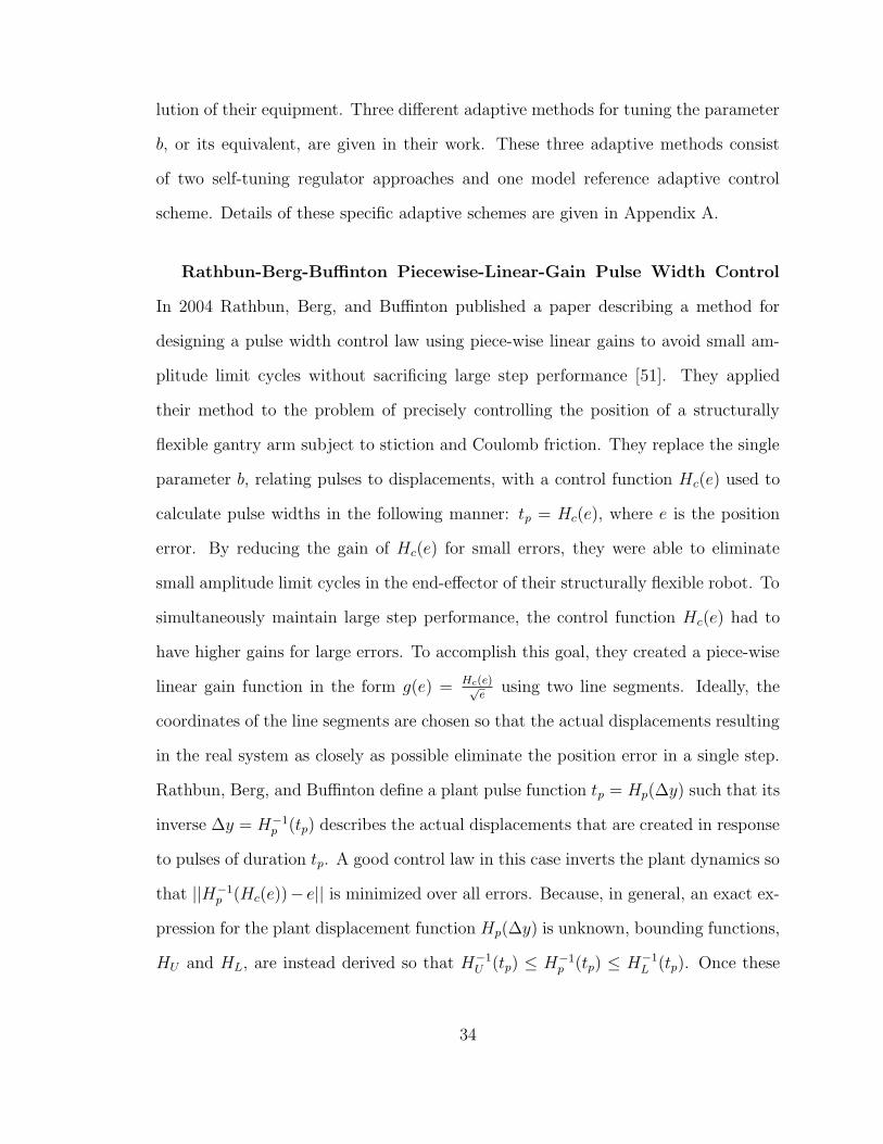
Rathbun-Berg-Buffinton Piecewise-Linear-Gain Pulse Width Control
In 2004 Rathbun, Berg, and Buffinton published a paper describing a method for
designing a pulse width control law using piece-wise linear gains to avoid small am-
plitude limit cycles without sacrificing large step performance [51]. They applied
their method to the problem of precisely controlling the position of a structurally
flexible gantry arm subject to stiction and Coulomb friction. They replace the single
parameter b, relating pulses to displacements, with a control function Hc(e) used to
calculate pulse widths in the following manner: tp = Hc(e), where e is the position
error. By reducing the gain of Hc(e) for small errors, they were able to eliminate
small amplitude limit cycles in the end-effector of their structurally flexible robot. To
simultaneously maintain large step performance, the control function Hc(e) had to
have higher gains for large errors. To accomplish this goal, they created a piece-wise
linear gain function in the form g(e) = Hc(e)√e
using two line segments. Ideally, the
coordinates of the line segments are chosen so that the actual displacements resulting
in the real system as closely as possible eliminate the position error in a single step.
Rathbun, Berg, and Buffinton define a plant pulse function tp = Hp(∆y) such that its
inverse ∆y = H−1p (tp) describes the actual displacements that are created in response
to pulses of duration tp. A good control law in this case inverts the plant dynamics so
that ||H−1p (Hc(e))− e|| is minimized over all errors. Because, in general, an exact ex-
pression for the plant displacement function Hp(∆y) is unknown, bounding functions,
HU and HL, are instead derived so that H−1U (tp) ≤ H−1
p (tp) ≤ H−1L (tp). Once these
34

upper and lower bound functions are known, Rathbun, Berg, and Buffinton provide
a method for selecting the coordinates of the line segments to define the piece-wise
linear gain function g(e) = Hc(e)√e
. Although deriving the lower and upper bound
functions can usually be derived based on first principles, the process is somewhat
tedious and depends on accurate identification of friction and actuator forces, as well
as accurate values for the masses in the system. No provision is made for changes in
payload.
Using this approach, Rathbun, Berg, and Buffinton demonstrate significant re-
ductions in ultimate positioning error when controlling the position of the robot’s
end-effector. They also improved performance by a factor of two as compared to a
constant gain pulse width control law. While effective, the method is neither adap-
tive, nor particularly easy to commission, requiring system parameters to be explicitly
identified before the coordinates of the piece-wise linear gain function can be set. A
method that is easier to commission is desired. In fact, a method that extends the
benefits of variable gains to fit even more complex displacement-pulse relations than
is possible with only two straight lines, that automatically initializing those gains,
and then adapts to changes in system parameters would be even more desirable.
35

3 Experimental Apparatus and Software
3.1 System Description
3.1.1 Mechanical Hardware
The system used to conduct the experiments consists of an Industrial Emulator manu-
factured by Educational Control Products, Model ECP 220. The ECP 220 is a rotary
system that can be mechanically reconfigured to emulate several different kinds of in-
dustrial systems on a small scale. A photograph of the system is shown in Figure 1.
The system consists of two three-phase brushless motors, two driven load wheels
whose moments of inertia can be varied with brass weights, a variable brake, and
several pulleys for connecting the motors to the loads through cogged belts. High
resolution optical encoders are used for feedback.
A single-phase, fixed-field, DC servo motor and linear motor amplifier were added
to the system for the purpose of conducting the experiments associated with this
work. A simplified schematic of the portion of the ECP 220 system used in conducting
experiments is shown in Figure 11. (Note that the right half the ECP 220 Industrial
Emulator shown in the photograph is not used for the experiments described in this
work.)
3.1.2 Equations of Motion
A free-body diagram of the ECP 220 Industrial Emulator is shown in Figure 12 where,
Jm and Jw are the respective moments of inertia of the motor and load wheel, Θm
36

Figure 11: ECP 220 Simplified Schematic
and Θw are the respective angular positions, τa is the actuation torque developed in
the motor, τmf and τwf are the friction torques, rm and rw are radii of the motor
and load wheel pulleys, T1 and T2 are the tensions in each side of the belt, ς is the
incremental stretch in the belt, and Kb is the spring constant of the belt.
T1
T2
T1
Kb
KbT
τ
τ a
Θr w
rm
τ
mf
m
Jw
wf
Jm
2
Θw
Figure 12: Free Body Diagram
37

The equations of motion representing the dynamics of the system can be found by
summing the moments on each inertia,
JmΘm = τa − τmf + rm(T1 − T2) (10)
JwΘw = −τwf + rw(T2 − T1) (11)
by calculating the incremental stretch per belt segment,
ς = rwΘw − rmΘm (12)
and finding the differential tension, T1 − T2, between the segments in the belt,
T1 − T2 = 2Kb ς (13)
Although the effort of actuation is developed in the motor, the load wheel is the
controlled entity. The compliance between the motor and load along with the multi-
ple sources of friction emulate characteristics found in many industrial applications.
Nonlinear friction arising from the motor brushes and variable brake provide an ad-
ditional challenge to controller design, but friction sources producing similar types of
friction can be found in many real machines.
3.1.3 Friction Equations
Several excellent models have been advanced in the last two decades which allow us to
predict the forces of friction with much greater fidelity. The LuGre friction model [17]
is able to predict the following friction behaviors:
• static friction
• Coulomb friction
38

• Stribeck effect
• Dahl compliance
• hysteresis in the force-velocity relation
• force rate dependent break-away friction
The LuGre model is defined by
s(ω) = sgn(ω)(
τc + (τs − τc)e−(ω/ωs)2
)
(14)
dz
dt= ω − σ0
ω
s(ω)z (15)
τf = σ0z + σ1dz
dt+ σ2ω (16)
where Equation 14 is known as the Stribeck curve, depending on angular velocity, ω,
that accounts for the combined effect of Coulomb friction torque, τc, static friction
torque, τs, and the transition between static and Coulomb friction values near the
Stribeck velocity, ωs. Equation 15 models the mean asperity deflection which helps to
model many of the friction effects described in Section 2. Here z is the mean asperity
deflection between the sliding surfaces; σ0 is torsional stiffness parameter relating the
torque developed by the asperities to the deflection z.
Equation 16 represents the composite LuGre friction torque that depends on Equa-
tions 14 and 15. The parameter σ1 is an asperity damping coefficient, and σ2 is the
usual viscous friction coefficient. Friction torques of the motor and load wheel, τmf
and τwf , in Equations 10 and 11 exhibit the type of friction given by τf in the LuGre
equations. Two sets of parameters, τc, τs, ωs, σ0, σ1, σ2 are needed to fully describe
the friction in the system: one set is needed for the motor, and the other for the load.
39

These several parameters will of course differ between the motor and load, and will
vary based on a number of factors such as position, belt tension, and temperature.
Controllers and control methods whose design and tuning must be delayed un-
til all system parameters are fully identified are the most difficult and expensive to
commission. Controllers and control methods that do not require full system identi-
fication, but which allow for at least a measure of self-tuning can be quite valuable
in the face of variations when best performance is desired on difficult to model or
unmodeled systems.
3.1.4 Motor Equations
The motor is a Clifton Precision PM DC Motor, Model: JDTH 2250 FN-1C. Perma-
nent magnets in the stator supply a fixed magnetic field; brushes supply current to
its rotating armature. Figure 13 shows a diagram of the motor model. The equations
for the dynamics of the motor are
τa = Kti (17)
dω
dt=
τa − τf
J(18)
di
dt= −Kt
Lω − R
Li + v (19)
ω =dΘm
dt(20)
where τa is the magnetic torque developed by the motor, Kt is the motor torque
constant, i is the electrical current, ω in the angular velocity of the motor shaft, τf is
40

K
xx
xx
ω
LR
+
_
+
_
ωvt
i
J
fτ
τa
Figure 13: Servo Motor
the friction torque within the motor that may be described by the LuGre equations
of the previous section, τa is the torque applied to the rest of the system, L is the
inductance of the motor windings, R is the electrical resistance of the windings and
brushes, and v is the voltage applied to the terminals of the motor.
3.1.5 Motor Amplifier
The Pulse Width Modulated (PWM) motor amplifier originally installed in the ECP
220 system was replaced with a a linear amplifier in order to gain high resolution,
reliable control over pulse durations. A linear voltage amplifier allows for precise con-
trol without interference from PWM circuitry. This replacement allowed arbitrarily
short pulses to be applied to the motor. The linear amplifier used for experiments was
based on a National Semiconductor LM12CL chip having the following specifications:
• ±10 A output current limit
• ±25 V output voltage swing
41

• a large signal rise time of less than 5 µs
• sufficient thermal conductance between its junction and case to allow for 80 W
of continuous power dissipation
The amplifier was wired in an inverting voltage feedback configuration to have an
unsaturated voltage gain Av = −5.08 volts/volt. During output saturation conditions,
the output voltage of the amplifier is limited to ±10.0 V. Saturation occurs when the
amplifier output voltage clamps against the power supply rails and no longer remains
a scaled copy of the input. When the input voltage becomes too large to be followed,
the output voltage clamps against the available power supply voltage levels. For these
experiments, the power supply voltages had to be limited to approximately half of
the amplifier’s voltage rating to safely handle the voltages associated with brushed
motor commutation and dynamic braking.
3.1.6 Transducers
To measure output positions, rotary incremental optical encoders are attached to the
shaft of the load wheel and the shaft of the motor. Encoder resolutions are 16000
and 4000 electrical counts per revolution respectively.
To measure actual current in the motor armature, a series sense resistor was
inserted in the motor amplifier circuit. The voltage across this sense resistor is pro-
portional to motor current and thus the developed motor torque. The value of the
sense resistor was carefully measured through live load testing to be 0.245 Ω with a
standard deviation of 0.0009 Ω. The torque constant of the motor was also carefully
measured in a series of torque calibration experiments to be 0.061 Nm/A with a stan-
dard deviation of 0.0014 Nm/A. Therefore, a 1.00 V measurement by the analog to
digital converter monitoring the series sense resistor implies a motor current of 4.08 A
and developed motor torque before brush and motor bearing losses of 0.249 Nm.
42

3.1.7 Signal Electronics
A US Digital PC7166 optical encoder interface is used to detect the direction and
count of encoder lines passing the optical encoder optics. The PC7166 card is used
to interface the optical encoder measurements to the control computer. This PC7166
card simultaneously reads 4 channels (in quadrature pairs) and maintains a 24 bit
counter for each channel yielding a count range of [-223, (223-1)]. This converts to
approximately ±524 revolutions before counter overflow or underflow when running
at the highest available resolution settings. A Computer Boards CIO-DAS08/JR-AO
is used for analog to digital conversion in reading the motor current sense voltage, as
well as for digital to analog conversion in generating the pulse voltages. This DAS08
card has an input and output resolution of 12 bits (1 in 4096) over a range of ±5 V
with a maximum sample rate of 20 kHz.
3.1.8 Sampling and Timing Resolution
The real-time kernel modules that are used to monitor and control all timing events
are based on an Intel Pentium III 450 MHz internal Time Stamp Counter (TSC)
having a resolution of 2.22 ns. TSC readings are converted into microseconds for all
experiments. All sampling times, pulse generation timings, and time stamps gener-
ated taken or developed in these experiments are rounded or truncated to the nearest
microsecond.
3.2 Real-Time Operating System Design
3.2.1 A New Kernel
Modern operating systems are typically of the multitasking type. A multitasking
operating system appears to simultaneously process many tasks at once. Most com-
43

puting hardware relies on a single processor, so in reality only one task may run at
once. Therefore, the operating system must divide the attention of the processor
between multiple processes. To accomplish multitasking, operating systems will typ-
ically divide time into slices. Each process is allowed to run within a given time slice
before being interrupted and rescheduled. At the end of each slice, the next scheduled
process is allowed to run. Most processes take several time slices to complete. The
order in which processes run is dictated by the operating system kernel.
The kernel generally attempts to give processes of highest priority a greater pro-
portion of the available time slices. However, to ensure that no process is completely
starved, even high priority processes are periodically interrupted by lower priority
processes. Why is the discussion of multitasking, scheduling, and priority impor-
tant? Any interruption of a real time process can be at worst catastrophic and at
best corrupt the data and control associated with the experiment. To ensure that
sampling occurs in a regular, periodic fashion, and even more importantly that the
control signals including such characteristics as pulse duration are accurately gener-
ated, the timing with which the control software executes must be exact and never
be pre-empted by other processes. For example, if a real-time control process were
running using a standard kernel and a full block of memory needed to be swapped to
disk, several tens of milliseconds of interruption to the real-time process could occur.
During this interruption, hundreds of measurement samples would likely be missed.
Worse yet, the generation of control signals would freeze at whatever voltage was
being applied at the moment when the interruption of the real-time process occurred.
This could lead to imprecise and erratic control at best. Even if the real-time control
process were given highest priority, most operating systems would still allow lower
priority processes to periodically interrupt the higher priority real-time processes.
44

There are great benefits however to being able to run a modern operating system
in conjunction with, or at least on the same machine as, a real-time control pro-
cess. These benefits include scheduling batch jobs using modern scripting languages,
streaming large data sets to disk, and starting, stopping, and monitoring processes
over a network. Perhaps the biggest incentive to finding a way to run a modern oper-
ating system in conjunction with a real-time control process is cost. Several powerful
open source operating systems, e.g. FreeBSD and Linux, are available at no cost and
run on commodity hardware. Open source software makes available to the public all
of the programming code needed to compile the software from scratch.
With open source software, nothing is hidden from view. This facilitates debug-
ging. The motivated engineer can study, tune, or modify an open source kernel or
open source applications that run on the kernel to fit his/her specific needs without
delays or service fees. If something is unclear in the system’s documentation, one can
resort to a direct analysis of the source code.
To efficiently test and compare several different control algorithms, the following
minimum requirements were defined for the real-time software needed to conduct the
experiments associated with this work:
• the real-time control processes are always given priority over non-real-time pro-
cess
• the real-time sampling of system outputs are never interrupted by lower priority
processes
• if a real-time process becomes ready for execution while another kernel process
is executing, then the real-time process can immediately interrupt or pre-empt
the other process (even before the end of the present time slice)
45

• when pre-emption does occur, the processor’s floating-point register contents (of
the interrupted process) are saved, allowing a full restoration once the real-time
process finishes execution—otherwise the real-time process will corrupt floating
point arithmetic of other processes
• an average jitter of less than 10 µs is required, where jitter is defined as short-
term variations between periodic events that do not occur at their ideal positions
in time
• sampling of all analog and optical encoder inputs must be possible at rates up
to or exceeding 10 kilosamples/second
• network communications, disk access, and other input/output processes will be
possible whenever all real-time processes are idle
To meet the above list of specifications, several alternatives were considered. Finally
a distribution of Linux was chosen for the base system. Version 2.4.23 of the Linux
kernel sources were downloaded and then patched with the Real Time Application In-
terface (RTAI) for Linux, using RTAI Kilauea Version 3.0, Revision 5. After patching
the sources, the kernel was re-compiled and re-installed.
3.2.2 Interfacing to the New Kernel
Although the newly created kernel met the above real-time specifications, additional
software was needed so that control commands and resulting response data could be
translated into a practical format. Also drivers for data acquisition cards had to be
written. To accomplish these goals, a scheme of layered processes were defined to
surround the real-time process in progressively higher layers of abstraction. These
layered processes are shown in Figure 14. The real-time processes are confined to
the innermost layer, in the figure, while the non-real-time processes are shown in the
46

outer three layers. In practice, the progressively layered design made verification and
development straightforward, and helped to make core components re-usable between
algorithms. In practice, the two innermost layers were combined into a single program,
but the conceptual separation was still evident and useful within that program.
response vectors from kernel are sent to standard out
FIFO TO STDIO TRANSLATOR
REALTIME KERNEL MODULE
BATCH CONTROL AND TRAJECTORY GENERATION
invokes realtime kernel modules specific to each control algorithmsearches/interpolates the control map to determine the width of each pulseupdates the pulse control map based on post pulse residuals
standard input is sent to kernel’s input FIFOtranslates between binary and ASCII formats
ADAPTIVE CONTROL SCRIPT
determines when to reset and warmup the systemqueues trajectory vectors into control scripts which in turn specifies the algorithm type
detects settlingreads and writes to and from FIFO’s
generates pulsesreads optical encodersexecutes realtime sampling schedule
Figure 14: Layered Processes
Even though non-real-time processes cannot be allowed to interrupt real-time
processes without data corruption or damage, the kernel memory is finite and must
periodically be streamed to disk if the process is to run without consuming all kernel
memory and without data loss. Since disk access usually requires a much longer
delay than can be tolerated by real-time control, an intermediate storage area, or
47

memory buffer, had to be created in order to pipe measurement data from the real-
time processes to the non-real-time disk storage utilities. Never missing a beat while
streaming data to standard I/O or disk turned out to be an important challenge. But
the challenge was met with satisfying results.
Many control algorithms can now be tested quickly and easily with standard
hardware. Furthermore, the layered process approach affords the benefits of using a
standard input and output routines that are familiar to most Unix users. Verification
and debugging times of the various algorithms were minimized because the input and
output and real-time functions were kept distinct and separate from the actual coding
of the algorithms.
48

4 Adaptive Impulse Control
4.1 Overview
The objective of Adaptive Impulse Control (AIC) method is to quickly move posi-
tioning machines from one point to the next without sacrificing precision. AIC is an
impulsive method. AIC is also adaptive; it is designed to improve its performance
with use. How does our review of friction in Chapter 2 inform the development of
the Adaptive Impulse Control approach?
Friction is multi-faceted. The force of friction depends of velocity, displacement,
acceleration, and path. Temperature and position dependence are also important
factors influencing the friction force. Therefore, calculating the energy required to
move from one point to the next in mechanical systems can be complex and depend
on many variables. But small displacements have been produced with repeatability
using impulsive control. The impulsive control approach can be simplified to the
calculation of single pulse per positioning event without requiring the measurement
or estimation of intra-pulse velocity or acceleration.
To control position over a wide range of displacements, pulses must be varied as a
function of desired step size. The relationship between pulse duration and step size is
seldom a simple function. A controller that automatically identifies this relationship
through online learning would be desirable. To map the complex relationship between
pulses and displacements for both fine and coarse moves, Adaptive Impulse Control
will therefore automatically tune a set of control parameters. Each control parameter
is a pulse value expected to produce a given displacement. During initialization,
49

a fixed set of log-spaced displacements are chosen for which pulse values are to be
learned. By using a log-spacing, a wide range of displacements can be covered for both
fine and coarse displacements. The pulse value expected to cause each displacement is
learned either by a short training exercise and by ongoing updates that progressively
refine the parameters.
To apply pulses for displacements not stored in the control map, the nearest stored
values are interpolated. After the interpolated pulse is applied, if the system did not
move exactly by the desired displacement, an optional update is performed. The
update attempts to correct only those specific pulse parameters that were used to
interpolate the most recently applied pulse.
When the stored relationship converges to the actual relationship of the machine,
each pulse applied to the system will be accurate. When each pulse is accurate, one
or few pulses will be needed to reach each desired destination. When fewer pulses
are needed, settling time is improved and efficiency is increased. Figure 15 shows an
overall block diagram of the AIC method. The main control loop and the adaptive
algorithm will now be briefly explained to introduce the rest of the chapter.
4.1.1 Main Control Loop
A reference position r is provided by the user or a supervisory program to the input of
the AIC controller. Control error e is calculated in the usual fashion as the difference
between the reference r and the output y. The control error is used to derive a index
value j that locates pulse information in the control map most nearly associated with
displacements equal to e. A pulse interpolation algorithm then calculates a scalar
pulse command p to cause a displacement e. This pulse command is sent to a pulse
generator that generates a single rectangular pulse of amplitude vp = sgn(p) Vsat
50

j
−1
q−1
Σ+
_ algorithm
pulse yr einterpolation
p mechanical
system
v
generatorpulseindex
encoder
µ
Σ+ _
sensitivityestimator
pulse
λupdate
algorithm
ε
vectorupdate
p
maplog−spaced
k−1j
q
Figure 15: AIC Block Diagram
and duration tp = |p|, where Vsat is a constant. The generated pulse generally causes
motion. Friction inherent in the system provides braking, as does the effect of dynamic
braking when motor voltage is again forced to zero. Each pulse will therefore cause
the system to step from one position to the next with a displacement that depends
on the size of the pulse.
If the calculation of the pulse is correct, then the system will move exactly to the
reference position r in a single step. When the calculation of the pulse is not ideal,
the system should still move closer to target so long as the initialization of the stored
parameters is reasonable. By repeating the process, multiple pulses can be used, each
progressively reducing the position error until the positioning tolerance is met.
4.1.2 Adaptive Algorithm
After a pulse is applied, the system settles on a new position, so long as the applied
pulse was long enough to cause motion. Some residual position error, ε, is likely
to remain after the pulse. Residual error measures the distance by which the last
51

pulse missed its intended displacement. If pulses are not producing their intended
displacements, then the residual error ε should be used to correct the pulse parameters
stored in the control map.
The first step in the update is to locate (or recall) the stored pulse parameters
that were responsible for generating the most recent pulse. AIC calculates a single
decimal index value j for this purpose. The integer values of j and j + 1 point to the
left and right bracketing parameters used to generate a pulse. The fractional part of
j gives the interpolation fraction. The delay operator q−1 is shown in Figure 15 to
indicate that a one step delay is applied the index value used in making the update.
The update is calculated after each pulse is applied (conceptually at the beginning
of the next pulse) and therefore should be applied to the parameters used one step
ago. The idea is that updates should apply specifically to the parameters that are
responsible for a particular residual error.
The next question is: By how much must a pulse change to produce a differential
unit of displacement? In other words, how sensitive is the system? We call this
the pulse sensitivity µ and define it as µ(d) = ∂p∂d
. Since the control map maintains
the most recent estimates of how pulses are related to given displacements, we can
numerically estimate the pulse sensitivity as a function of displacement based on the
stored map values.
Knowing the residual error and knowing the sensitivity of the system are enough
to estimate a correction. The update is simply µε. Somehow this correction must
be distributed among the pulse parameters in the control map. Several ways for
distributing the correction are explained in the sections ahead. But essentially we
are producing an update vector uk. This update vector typically has two non-zero
elements whose indices match the pulse parameters that are to be corrected. The
correction is applied as pk+1 = pk + uk.
52

In practice, a learning parameter λ is also applied to throttle the learning. If the
residual error associated with the last pulse were the result of a random disturbance or
measurement noise, rather than a poorly tuned control map, then a more conservative
correction would be desirable. A throttled correction is λµε where λ ∈ [0, 1]. When
λ is close to zero, the parameters learned in the past are not so quickly forgotten.
Finally, as always, it is important to consider the issue of stability. Before actually
distributing the throttled correction into the control map, constraints for guaranteeing
stability can be applied. Chapter 6 provides a derivation of stability constraints that
can be applied to results of pulse interpolations in the main loop and to pulse updates
made by the adaptive algorithm. We now look at the AIC method in greater detail.
4.2 Description of the New Method
The Adaptive Impulse Control (AIC) method can be implemented in three major
segments: start up, main loop, and shut down. Each segment is composed of several
subroutines. Figures 16 through 18 show the layout, order, and path forks between
subroutines.
53

1
start AIC
activate realtime modules
open FIFO’s
open data files
initialize the control table
read initial conditions
Figure 16: Start Up
54

try again
1
move on to nexttolerance met;
reference
r == EOF
read r
YES
read y
reset k
increment k
update
apply p
lookup p
calculate e
| e | < TOL
k <= MAX
report difficulty
NO
YES
YES
NO
NO
read y after settling
2
read transient response
report
Figure 17: Main Loop
55

deactivate realtime modules
zero amplifier
flush FIFO’s
close data files
plot responses
end AIC
2
Figure 18: Shutdown
56

activate real-time modules The first subroutine in the AIC method loads the real-
time kernel modules. The real-time modules are written to handle tasks that execute
according to strict timing deadlines that cannot be missed. Timing critical tasks
handled by the real-time modules include
• starting and ending the pulses
• sampling the optical encoder card and the analog to digital converter at precisely
spaced intervals
• measuring the precise time at which samples are taken
• detecting settling, i.e. determining when the system has come to rest after each
pulse
• buffering the data into memory buffers for later disk storage
Sampling must occur before, during, and after each pulse to capture all the transients.
A pulse seldom ends precisely in synchronization with a sampling event. Therefore,
the real-time modules must mix fractional and integral event times in order to suc-
cessfully apply arbitrarily long pulses without skewing the integrally spaced sample
schedule. This includes the case of a pulse whose duration is shorter than single sam-
ple period. The real-time modules are written to carefully juggle both the sampling
and pulse application schedules even though only a single timer and processor are
available.
Several different kernel modules are used to execute the various real-time events:
one module is used to install the hardware abstraction layer, one for the a real-
time scheduler, one for the first-in-first-out (FIFO) memory handler, and one for
the specific control algorithm that is to be run. Once the modules are installed, all
interrupt requests are channeled through the real time application interface. Normal
57

interrupt service routines associated with the base operating system are delayed until
all real-time processing is satisfied. This ensures all real-time functions execute on-
time without interference from other processes.
open FIFO’s Since writing to disk is an asynchronous, non-real-time process, the
real-time control process cannot wait for measurement data to be recorded on a disk
drive. In fact, any pending disk access must be put in the background while real-time
events are occurring. Otherwise control interruptions or data loss will occur, because
only a single processor is available to handle all operations. To capture the data in
real-time then, the sampled data is first buffered into first-in-first-out (FIFO) kernel
memory buffer. Ten megabytes of kernel memory are allocated for this buffer. Data
from the optical encoder interface reading load and motor angle, as well as data from
the analog to digital converter sensing motor current, and other variables are read
at 10 kilosamples/second. In all, 6 system variables of 4 bytes each in little-endian
format are streamed into the FIFO’s. Little-endian format assigns low order bits to
the first byte of a digital word and high order bits to the last byte of a digital word.
This allows small integers of different precisions to be stored in the same memory
location.
open data files Data files should be opened before any data is collected. After each
pulse, event data is appended to the data files. This design allows for trajectories
of indefinite length to be recorded without FIFO overflow. If instead, we instead
attempt to store the data from all pulses at the end of the run, the FIFO would
overflow before all the data were collected. Some control methods require vastly
more steps than others to reach the same destination. Therefore, opening files at this
stage is crucial to avoiding overflow of the FIFO buffers. During idle periods of the
real-time process, the data is streamed into the open data files after being translated
into ASCII format by the non-real-time control scripts. The ASCII format, while less
58

efficient in terms of storage, allows many different programs to post-process the data
and leaves the data in a human-readable form.
initialize the control table The control table provides a map between system dis-
placements and pulse widths. To calculate how long a pulse should be applied in
order to move the system a given distance, the control table is consulted. The lookup
section below explains how pulses are calculated after initialization. This section
explains only the initialization. For each displacement value, a corresponding pulse
value will be stored in the control table. Since memory is limited, a limited number of
displacement-pulse pairs can be recorded. Therefore, a fixed number of displacements
are initially chosen for which corresponding pulse values will later be learned.
Why choose a fixed set of distances and learn the associated pulse values, instead
of choosing a fixed set of pulse values and learning the associated displacements
caused by those pulses? Recall that in general, the control problem is to find the
control effort or pulse value required to move the system a specified distance, not vice
versa. It is also preferred to have a reliable spacing on the displacement values. If we
instead forced a regular spacing on pulse values and proceed to learn the displacements
associated with those pulses then we encounter the problem of multiple pulse values
so small that the system does not break free or move at all. The distance travel by
applying an identical pulse differs slightly from run to run, even when initial conditions
are apparently identical. Multiple zeros in the abscissa data present a challenge to
most interpolation algorithms. We prefer instead to specify an abscissa displacement
value and have the interpolation algorithm return an ordinate pulse value. Therefore,
a fixed number of regularly spaced displacements are chosen.
59

One way to cover a wide range while preserving fine resolution is to use log-spacing
on the displacement values. A possible set of displacements is
d =
[−100000
−10000
−1000
−100
−10
−1
0
1
10
100
1000
10000
100000
(21)
measured in optical encoder counts. These are the displacement values for which
pulses will be learned. Other sets of displacements can be chosen. For example,
assuming that system responses are symmetric in the forward and reverse directions
would cut the table in half. To find the pulse values, two options exist. The first option
assumes no prior knowledge of system responses. The second uses prior knowledge
recorded from earlier system responses.
60

In the case where prior system responses are either unavailable or ignored, various
training pulses are applied and the displacements recorded and interpolated into the
control table. A set of training pulses pt often used to train the system is
pt =
−100
100
1000
−1000
10000
−10000
100000
−100000
1000000
−1000000
(22)
measured in microseconds. A negative pulse value does not imply negative duration,
but rather negative amplitude. Applying these pulse values, one by one with the
control loop open, will cause the system to move various distances, none of which will
likely match any values in the previously specified d vector exactly. But the distances
are recorded and then interpolated so that not even the number of values in the initial
control table pulse vector, p0, and the training vector, pt, need be the same.
61

For example, the displacements in one training session using pulses in the above
specified pt vector, yielded displacements of
dT
t= [−1, 1,−32, 46,−800, 806,−9336, 9109,−99185, 96848] (23)
The (dt,pt) training data is then interpolated at the regularly log-spaced values in
d to yield an initial set of control values:
p0 =
−1008164
−106651
−12109
−1797
−361
−100
0
100
280
1639
12103
109140
1032332
(24)
62

The initial control table provides a basis for initial control. A pulse value for
any displacement can be interpolated over the system range. Together the d and p0
vectors then form the initial control table:
(d,p0) =
−100000 −1008164
−10000 −106651
−1000 −12109
−100 −1797
−10 −361
−1 −100
0 0
1 100
10 280
100 1639
1000 12103
10000 109140
100000 1032332
(25)
Log-spacing allows the whole range to be covered using limited memory without
sacrificing granularity at the finest displacements. The displacement vector d is now
fixed, but elements of the pulse vector, pk, column of the table can be incrementally
improved with system use if needed. (See update section below.) The subscript k is
incremented by one after every pulse.
Here only twelve training pulses were needed to initialize the control table. If more
training pulses were used, then an even more accurate set of initial control values could
be obtained. Due to the fact that the training pulses were applied only a single time,
no multi-point averaging has yet occurred. Furthermore, imperfections in these values
63

may be present from initial interpolation. The online update mechanism described
below (see update subroutine) will refine the (d, p) paired values with system use. At
this stage of control, it is sufficient to apply a few pulses if no prior information about
the system is available. Otherwise, the (d,p0) table could have been pre-generated
offline using a dynamic system model. Once of the strengths of the present approach
is that it can be applied to position control systems with or without completely
identified system models.
In the case where prior system responses are available, the above procedure can
be bypassed and the most recent (d,p) data from previous runs can be loaded instead.
Any changes in system parameters, payload or environmental changes that have oc-
curred since the last run will be corrected through the ongoing tuning that occurs
from the update subroutine.
read initial conditions The initial position of the system is recorded at the be-
ginning of each run before any pulse control begins. The position of the system is
measured by optical encoders. The contents of the registers on the optical encoder
card are translated from byte data into signed integer values. The resolution is 16000
counts/revolution on the load. The optical encoder card in this system maintains 24
digital bits of precision for ±524 revolutions before overflow.
read the reference command References can be sent to the controller either through
the keyboard or by redirecting a trajectory file into the standard input of the main
control script. The reference (or target) variable is known as r. The outer control
loop terminates when an end-of-file is encountered or a Ctrl-D is read. The reference
is read in units of encoder counts.
inner control loop Each new reference value being sent to the controller may result
in zero or more pulses. If the system is already at the newly specified position, then
no pulses will be sent. Otherwise at least one pulse will be applied. Once the system
64

achieves the new position within a specified tolerance using one or more pulses, the
controller will wait for the next reference command to be issued and continue running
the inner loop.
read yi The initial position of the system load, yi, is read before each pulse is
applied. The reading is in units of encoder counts. There are 16000 encoder counts
per revolution on the load wheel.
calculate ei The initial control error, ei, is the difference between the reference
and the initial position,
ei = r − yi (26)
lookup p The pulse value needed to move the system to the reference position,
r, ideally produces a displacement that, in a single step, completely eliminates the
initial control error, ei. In other words the ideal pulse value produces a displacement
from yi of d = ei.
Since an analytical function p = p(d, ...) is in general a complicated function whose
parameters are expensive to fully identify, we seek an alternative to full identification
of a system model and the subsequent controller design. We can directly learn the
pulse values needed to move a given set of displacements. Perhaps the most efficient
and inexpensive way to obtain pulse values p for any needed d on the operating range
is through use and tuning of a lookup table.
To cover a wide range spanning on the order of four to six orders of magnitude
of displacement without using an enormous amount of memory, a log-spacing scheme
like that shown in Equation 21 is used to define the set of displacements for which
pulse values will be learned. This table can be cut in half if the system is known to
behave symmetrically in both the forward and reverse directions.
An important distinction of the AIC method as compared to other adaptive im-
pulse control control methods is how AIC’s use of interpolation frees it from the
65

normal constraints of generating a linear or low-order polynomial control law that
must apply globally. Other methods typically tune one or a few parameters in a
single control law (a set of gains or a set of polynomial coefficients) that must operate
globally. AIC instead allows for independent adjustment of an arbitrary number of
control points. Adjustments of pulse values for the smallest displacement need not
affect coarse control in any way. This is true even if updates are not enabled. The
approach allows for localized optimization that is much more efficient and effective
than global tuning. The trade-off is that a modest amount of memory is needed (the
engineer can make the control map as granular as he/she wishes), and many points
imply the need for some sort of automated tuning.
After a table like that shown in Equation 25 has been initialized, a pulse value
can be found by either looking up the nearest neighboring point, or by interpolating
between the nearest neighboring points. In the AIC method, any of several methods
of interpolation during pulse lookup can be used in looking up p from the control
table.
Once the pulse value has been interpolated, it may optionally be truncated for
stability according to the following rule:
if |p| > 2√
|d|/B, then set p = sgn(d) 2√
|d|/B (27)
where B is a parameter for guaranteeing stability. See Chapter 6 for additional details.
apply p Once the desired pulse value is known, a pulse signal will be generated
by the digital to analog converter in the computer and sent to the input of the motor
amplifier. Pulse duration, tp, is equated to the magnitude of the pulse value, |p|.
Pulse amplitude depends on the sign of the pulse value. If the pulse value is positive,
then this indicates the need for forward motion. On the other hand, if the pulse
66

value is negative, this implies the need for reverse motion. In equation form, pulse
duration, tp, and pulse amplitude, vp are given by:
tp = |p| [microseconds]
vp = sgn(p) · Vsat [volts]
(28)
where Vsat is the saturation voltage of the amplifier. The positive and negative am-
plifier saturation voltages are symmetric in this system. Vsat, the maximum voltage
magnitude available, is chosen as the positive and negative rectangular pulse magni-
tude in pursuit of the quickest possible motions and crispest start and stop transitions.
For illustration of how pulses are generated, consider two pulse values: p1 = 3333
and p2 = −3333. The magnitude |p1| = 3333 implies a desired pulse duration of
3333 µs; the sign: sgn(p1) = 1, implies a positive fixed amplitude of +10.0 V. Together
these define a rectangular positive pulse intended to cause forward motion. Similarly,
the duration of the second pulse is 3333 µs, but its amplitude will have a negative
saturation value of −10.0 V, since sgn(p2) = −1. The rectangular negative pulse is
intended to cause reverse motion. The first plot of Figure 19 shows waveforms sent
to the motor based on these two pulse values; the second plot shows the resulting
torque developed in the motor.
The current in the motor is a response to the voltage on its terminals as applied by
the motor amplifier. The current response is also a function of the voltage generated
by the motor armature. Rotational velocities of the motor are normally quite small for
short moves, so the back emf is often negligible. For medium to large moves however,
dynamic braking can occur. Dynamic braking results when the motor amplifier forces
the voltage across the motor terminals to return to zero after a pulse. While the motor
is still spinning, the voltage generated internally will suddenly exceed the terminal
voltage, resulting in a current reversal and a braking torque. This braking torque helps
67

0.06 0.08 0.1 0.12 0.14 0.16 0.18
−10
−5
0
5
10
volts
0.06 0.08 0.1 0.12 0.14 0.16 0.18
−0.2
−0.1
0
0.1
0.2
0.3
new
ton−
met
ers
seconds
Figure 19: Example of Short Voltage Pulses and the Resulting Motor Torque
to quickly dissipate the kinetic energy even though the pulse initiating the original
motion was not followed by an explicit ‘braking’ pulse, but only a forced zeroing of
the voltage across the motor terminals. The reversal of torque is evident after the first
pulses shown in Figures 31 and 34 of the results chapter of this dissertation. With or
without dynamic braking, the resulting torque developed by the fixed-field DC motor
used in this work was verified to be directly proportional to the actual current in the
motor, with a torque constant Kt = 0.061 Nm/A. The electrical time constant of the
motor is L/R = 1.403 ms with R = 1.896 Ω and L = 2.660 mH.
In order to generate accurate timing, the real-time kernel module handles com-
munication with the digital to analog converter. It was important that fractional
sample period pulses are accurately generated. In other words, if the sampling period
T = 100 µs and p = 111, then the generated pulse will shut off 11 µs after the first
68

sample period, in between the normally scheduled sample times of 100 µs and 200 µs.
The real-time kernel module juggles pulse control with sample timing to keep both
on schedule. By developing the real-time control module in this way, artificial lim-
its are not imposed on pulse resolution and resulting displacement resolution by the
software. Any limits on displacement resolution are therefore due to the dynamics of
the system and friction physics.
read the transient response Measurements of position and motor current are made
every 100 µs during and after each pulse. Sampling continues after each pulse until all
transients have decayed. The samples are buffered into the FIFO buffers in real-time.
The contents of the FIFO’s are then asynchronously stored and post-processed by
non-real-time operating system processes.
read yf The post-pulse settling position is read after the pulse has been applied
and transients have decayed. To detect the end of motion caused by each pulse, a
moving sample window is applied. Once the last 200 samples in the moving window
are found to be identical, yf is assigned the value of the last position reading.
calculate ef The post-pulse or residual control error is calculated as
ef = r − yf (29)
perform an update In order to gain and maintain optimal tuning of the control
table, an optional update is applied to the control table at the end of every pulse re-
sponse. If pulses are not creating the desired displacements, we can probably improve
the control table. We begin with a simple update of the form
pγ,k+1 = pγ,k + λΥ (30)
69

as if this update could be applied anywhere on an interpolated control curve. The ‘γ’
subscript implies the interpolated virtual position in the control table at which the
displacement would exactly equal the error beginning at the time step, d = ei. λ is
a unit-less adaptation rate, while Υ is defined as a pro-forma update in microseconds
as the product of two important terms
Υ ≡ µef (31)
where ef is the residual error defined in Equation 29 with units of encoder counts,
and µ is the pulse sensitivity
µ ≡ ∂p
∂d(32)
with units of microseconds per encoder count. The pulse sensitivity gives an indica-
tion of how much a pulse value must change in order to effect a different amount of
displacement. This sensitivity depends on displacement since p = p(d, ...) is in gen-
eral nonlinear. The relationship between pulse values and displacement is especially
nonlinear in the transition between stick-slip and sliding motion. Pulse generation
is most affected by the exponential rise time of current in the servo motor for very
short pulses. Both of these phenomena occur when making fine displacements. The
residual error, ef , indicates the amount of displacement needed in the ideal correction.
Often an estimate of µ will be estimated at a control error associated with the last
pulse, as in
µ(ei,k) ≈∂p
∂d
∣
∣
∣
∣
d=ei,k
(33)
The adjective “pro-forma” in pro-forma update implies we are making the calcu-
lation as if we could apply the update at a control table displacement exactly equal
to the value interpolated during the pulse lookup process, even though this exact
70

displacement value is not likely to appear in the control table. Once the pro-forma
update, Υ, has been calculated, it must be distributed by one of several possible
methods among points in the control table. Section 4.5 will describe various methods
for distributing the correction.
Note that if µ and λ are considered rates of adaptation or learning, although λ
may be a scalar constant, µ = µ(d, ...) is a strong function of the desired displacement
step size. Thus, we are defining a variable adaptive law to govern corrections. See
Section 4.4 for an explanation of methods used for estimating µ(d) from control table
data.
Hence not only does the approach defined in Equations 30 to 32 indicate an
update for tuning fine control values separately from coarse control (see Section 4.5
for details), but we are also defining a adaptation law that depends on the slope of p(d)
with respect to the desired displacement d. In other words, we have proposed a system
that not only learns, but learns how fast to learn. Chapter 5, shows how the AIC
compares to other impulsive methods from an adaptive point of view, and Chapter 6
gives a necessary criterion for guaranteeing stability when certain assumptions about
the mechanical system can be made. Applying (27) on all updates and interpolations
is sufficient for guaranteeing stability.
report data After each pulse, a vector of [r, yi, ei, p, δ, ef , tf ] is appended to the
data record for later analysis.
increment the step counters An overall iteration counter, k, is incremented after
every pulse event. A specific iteration counter, n, is also maintained. The specific
iteration counter, n, tracks the number of pulses needed to reach each reference within
the specified tolerance; it is incremented once for each pulse applied since the new
reference was read. This is needed since, usually at least a few pulses are needed to
reach each new reference with the tolerance. The n counter only gets reset if one
71

of the two break conditions below occur; k gets reset only when the entire control
program is restarted. n is a crucial figure of merit; it is the number of steps needed
to reach each reference. n should be as low as possible.
break if the tolerance has been met A break in the inner loop occurs when |ef | <
tol. This action allows the main loop to read in a new reference and the inner loop
to begin again.
break if the maximum number of trials has been exhausted A break in the inner
loop occurs, with an optional program exit, when n > nmax where nmax is the maxi-
mum number of allowed pulse attempts per reference. nmax is usually set to a number
between 20 and 200.
zero the amplifier In order to foster safe exit conditions, a voltage of zero is sent
to the amplifier input just prior to program termination.
destroy the FIFO’s Since the report subroutine has already appended all neces-
sary real-time response data to the open data files and the control program no longer
requires the asynchronous communication channel between the real-time and non-
real-time processes, the first-in-first-out buffers are destroyed in order to free kernel
memory.
deactivate real-time modules At this stage the real-time kernel modules can be
removed from the kernel, allowing regular non-real-time operating system processes
to run according to normal interrupt schedules, without interference from real-time
processes.
close data files All open data files are closed and data is written to disk.
generate response plots Several browser readable plots are automatically gener-
ated at the end of each run.
72

Having reviewed each of the subroutines of the Adaptive Impulse Control (AIC)
algorithm, we now look at underlying methods of interpolation, sensitivity estimation,
and update distribution in greater depth.
4.3 Interpolation Methods for Pulse Lookups
Under AIC control, whenever the system needs to move to a new position, a pulse
value must be calculated. Using the desired displacement and values in the control
table, several methods are available for looking up and calculating the pulse value.
Nearest Neighbor Lookup The simplest option for using the control table
to find a pulse value is to perform no interpolation at all. Instead the pulse lookup
consists of simply looking up the nearest point in the control table and using that
pulse value directly to generate the pulse sent to the motor amplifier. The nearest
point, measured in terms of the difference between desired and stored displacements,
can be found according to the following equations:
p = pj (34)
where
j = arg minj=1,...,N
||dj − ej|| (35)
Recall that the data in the control table covers several orders of magnitude of
displacement. Since we prefer a sparse table in order to limit the number of control
points to be stored and learned, large gaps should exist in the table. Unless we revert
to linear spacing and substantially increase the number of points in the control table,
then the nearest neighbor lookup is likely to produce pulse values that are not ideal
because of the large distances that will exist in the table between discretely stored
73

points. But the nearest neighbor lookup is simple, very fast, and can be made to
work if the control table is made sufficiently dense.
Linear Interpolation on Raw Data The simplest interpolation method is
linear interpolation. We denote linear interpolation by
yγ = interp(x,y, xγ) (36)
where x is a vector of abscissa values whose elements must be sorted and stored in
monotonic order, whose minimum value is x1 and maximum is xmax, whose index
ranges from 1 to jmax, y is a vector whose elements are the associated ordinate values
known to correspond to those in x, xγ is the abscissa value at which we wish to
estimate an ordinate value, yγ, by interpolation. Linear interpolation is then done
by:
if xγ ≥ xmax,
j = jmax − 1
else if xγ < x1,
j = 1
else
set j to the maximum j for which xj ≤ xγ
(37)
ξ =x − xj
xj+1 − xj
, xj+1 6= xj (38)
yγ = yj + ξ · (yj+1 − yj) (39)
For convenience in later discussion, we call ξ the interpolation variable. Linear inter-
polation is simple and fast. The disadvantage of linear interpolation is that it poorly
fits curved functions when the spacing between stored points is large.
74

Note that functions that have straight sections when plotted on linear scales may
or may not appear curved on log-log axes. Functions of the class y = xa + b appear
straight on log-log axes for all a ∈ <, b = 0. However if both a and b are nonzero,
even when a = 1, the function will appear curved on log-log axes. See Figures 20 and
21 for a comparative illustration.
Piecewise Cubic Hermite Interpolation A smoother fit to curved functions
can be found by using a Piecewise Cubic Hermite Interpolation Polynomial. A cubic
polynomial is used to span between each successive pair of points. Each section of
the curve will have a distinct set of coefficients. By allowing a piecewise fit, low order
polynomials can be used. Polynomials of order of three are chosen, so four coefficients
are needed on each section. To solve for four coefficients, four conditions need to be
required. The first two conditions are the obvious conditions that the polynomial
must pass through the left and right end points established by the known data. The
other two conditions are based on choosing slope values in some way. Functions that
satisfy interpolation conditions on derivatives are known an Hermite interpolants [38].
One of the key concerns over how these last two conditions are chosen in order to
establish the polynomial coefficients for each section relate to stability of AIC. The
update law of AIC depends on pulse sensitivity. If the known data is monotonic,
then we hope that the interpolating polynomial is also everywhere monotonic. If
such a relationship between the raw data and the interpolating polynomials can be
preserved, then we can with some confidence numerically or analytically differentiate
the interpolating polynomials to obtain estimates of the pulse sensitivity. On the other
hand, due to overshoot and oscillations that easily arise when fitting polynomials
to data, several sign inversions may result that destroy our ability to rely on the
polynomial interpolations for calculating the AIC adaptation rates.
75

Fortunately, a shape-preserving method was recently introduced into MatlabTM
that is not only visually pleasing, but that also preserves monotonicity of the inter-
polants when raw data supplied to the method is itself monotonic. The method is
based on a program written earlier in Fortran by Fritsch and Carlson described by
Kahaner, Moler, and Nash [35]. It is referred to as the pchip method. This method
establishes the following slope conditions:
1. If the first differences in the raw data on either side of a data point are op-
posite in sign, or if either of them is zero, then the slopes of the interpolating
polynomials on each side of the point are forced to be zero at that point.
2. If the first differences in the raw data are of the same sign, and neither is zero,
then the slopes of the interpolating polynomials on each side of the point are
forced to match the harmonic mean of the two discrete slopes
1
mj
=1
2
(
1
µj−1
+1
µj
)
(40)
where mj is the slope the polynomials are required to have at the j th point
based on the µj−1 and µj first differences in the raw data on either side of the
point.
Slopes at either end of the overall data set require a special one-sided slope evaluations
(usually based on a three point method). Once the above four conditions (two on
endpoint values and endpoint slopes are established), then equations can be solved to
evaluate the pertinent polynomial coefficients. Once the polynomial coefficients are
known, then finally interpolants can be found by evaluating the resulting polynomial
at specific points.
An example comparing the pchip interpolation method with other interpolation
methods using actual control map data is shown in Figures 20 and 21. These figures
76

represent identical information. However, the first pair of plots are done on linearly
scaled axes; the second pair on logarithmically scaled axes. Each plot pair consists of
a wide view (on the left) and a zoomed view (on the right). Note that log-log plots
cannot display negative data. Therefore, only the first quadrant of Figure 20 can be
displayed in Figure 21.
−1 −0.5 0 0.5 1
x 105
−1.5
−1
−0.5
0
0.5
1
1.5x 10
6
displacement [encoder counts]
puls
e va
lue
[mic
rose
cond
s]
interpolation methods
nearest−neighborlinearpchiplog−log interp
0 50 100 150−2000
0
2000
4000
6000
8000
10000
displacement [encoder counts]
puls
e va
lue
[mic
rose
cond
s]
zoomed view
nearest−neighborlinearpchiplog−log interp
Figure 20: Interpolation Methods for Pulse Lookups
Log-Log Interpolation While the pchip interpolation method does have nice
properties and is quite useful for simulations, the implementation of pchip in real-time
control hardware is somewhat cumbersome. For actual AIC implementation, a simpler
77

100
105
103
104
105
106
107
displacement [encoder counts]
puls
e va
lue
[mic
rose
cond
s]
interpolation methods, log−log axes
nearest−neighborlinearpchiplog−log interp
100
101
102
103
104
displacement [encoder counts]
puls
e va
lue
[mic
rose
cond
s]
zoomed view
nearest−neighborlinearpchiplog−log interp
Figure 21: Interpolation Methods for Pulse Lookups on Log-Log Axes
method was applied to interpolate curved data over widely variable, log-spaced spans.
This method, will be referred to as log-log interpolation, and implemented as follows:
1. Read in the abscissa value x for which an ordinate value is to be found by
interpolation.
2. Find the bracketing left and right index values.
3. Take the logarithm of absolute values of each abscissa and ordinate values, as
in:
X = loga(|x|) (41)
78

4. Linearly interpolate on the transformed values to find Y .
5. Inverse transform by raising the logarithm base by the power of the transformed
interpolant Y , and re-apply the sign of the nearest original ordinate yn:
y = sgn(yn) · aY (42)
6. Return y.
An example comparing this log-log interpolation method with other interpolation
methods using actual control map data is shown in Figures 20 and 21. Note the
similarity to the pchip interpolation method. The next table, Table 2, summarizes
methods for looking up data from the control table. Because of its high fit quality
Table 2: Pertinent Methods for Fitting Data
Lookup Method Transformation Interpolation Method Fit Quality Complexitynearest-neighbor lookup none none low low
linear interpolation none linear moderate lowlog-log interpolation logarithmic linear high moderatepchip interpolation none piecewise cubic Hermite high high
and moderate complexity, the log-log interpolation method is used for AIC pulse
lookups, unless otherwise noted.
4.4 Estimating Pulse Sensitivity
Two methods have been successful in practice for estimating the sensitivity of pulses
to a unit change of displacement, µ. The first is based on taking the derivative of an
estimated relationship of pulses to displacements:
p(d) = A · sgn(d)√
|d| (43)
79

where A is a scalar coefficient found by inserting the most up-to-date control values
into
A =1
nt
nt∑
j=1
|pj|√
|dj|, dj 6= 0 (44)
nt is the number of nonzero training pairs used in the estimate. Then the estimated
pulse sensitivity function is then found by taking the derivative of p(d) with respect to
d and adding a special case to handle the singularity at zero. To bridge the singularity
near the origin, we define µ(0) as the average of the closest two values that can be
measured near zero, namely µ(−1) and µ(1). Due to the digital nature of the raw
position measurement the smallest values near zero that can be measured are plus
and minus one encoder count. Also note that µ(0) seldom needs to be evaluated since
p(0) = 0 usually never needs correction in most positioning systems.
µ(d) =
A
2√
|d|d 6= 0
A2
d = 0
(45)
Figure 22 shows the nature of p(d) and µ(d) when using Equations 43 through 45.
Note that the curve appears to poorly fit the outer four points; however, equal weight-
ing is given to each point, and many points are found near the origin. Those points
near the origin are the ones that most affect fine position control. If they are dis-
counted, then hunting during ultra-fine positioning is likely to occur and settling
times will significantly increase when working within tight tolerances.
80
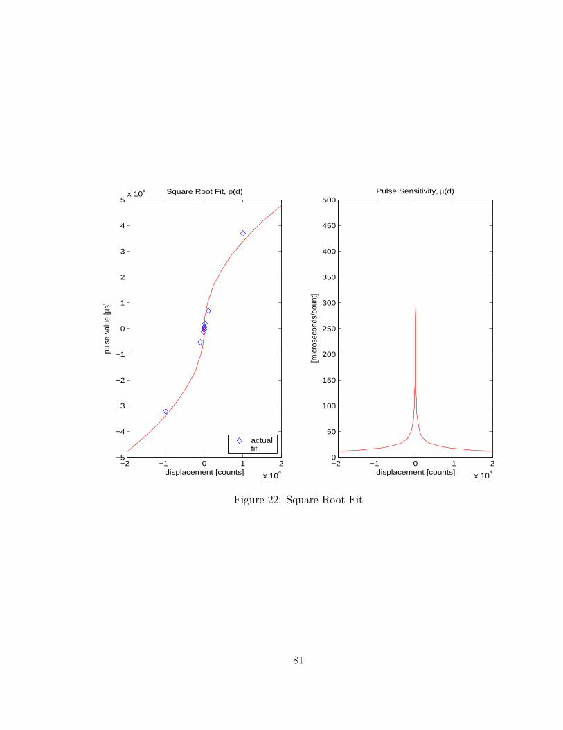
−2 −1 0 1 2
x 104
−5
−4
−3
−2
−1
0
1
2
3
4
5x 10
5
puls
e va
lue
[µs]
displacement [counts]
Square Root Fit, p(d)
actualfit
−2 −1 0 1 2
x 104
0
50
100
150
200
250
300
350
400
450
500Pulse Sensitivity, µ(d)
[mic
rose
cond
s/co
unt]
displacement [counts]
Figure 22: Square Root Fit
81

The second pulse sensitivity estimation method builds on the first. The first
method put full weight on the most recently recorded control table values. When
environmental disturbances or measurement noise is significant, it can be helpful to
put more weight on the historical average. A simple filter that provides an adjustable
balance between current and historical values can be implemented by making the
following calculation during each update:
Ak = (1 − α)Ak−1 +α
nt
nt∑
j=1
|pj|√
|dj|, dj 6= 0 (46)
where α ∈ [0, 1] is set close to zero when historical data is to be weighted heavily, and
close to one when recent data should carry more weight.
4.5 Update Distribution Methods
After an update Υ has been calculated by Equation 31, the question arises as to
how this update will be distributed among the sparse number of discrete points in
the control table; the attempted displacement will rarely align precisely with one of
the log-spaced displacement values in the control table. Interpolation is generally
used during the pulse lookup process, so during the update process should not the
update be applied by some sort of distribution to the control points that were used
in calculating the pulse? The answer to this question determines a balance between
adaptation law complexity and fairness of distribution of the update.
One Point Update The simplest distribution, of course, is to apply the entire
update to the nearest control point. The nearest control point can be found by first
calculating a decimal index value:
jγ = interp(d, j, ei); (47)
82

where the ‘γ’ subscript implies a virtual position in the table, and linear interpolation
is defined in Equations 36 through 39. The index value jγ is then rounded the nearest
integer to identify the actual index value that points to the nearest control point:
j = round(jγ) (48)
Equation 48 gives the index value used to determine which pulse value in the table
is updated. The update consists of applying the entire update to one point:
pj,k+1 = pj,k + λΥk (49)
where k is the iteration count that increase by one with each pulse application. Fig-
ure 23 shows an example of this nearest neighbor, one point approach where λ = 1.
The nearest point is over-corrected, the second closest point receives no correction at
all, but the update is simple.
83

−100 −50 0 50 100 150 200 250−3000
−2000
−1000
0
1000
2000
3000
4000
5000
6000One Point Update
displacement [encoder counts]
puls
e va
lue
[mic
rose
cond
s]
pre−updatepost−updateinitial lookuppro−forma update
Figure 23: One Point Update, Nearest Neighbor
84

Global Amplification: The All Point Update Instead of changing a single
point, it may desirable to amplify or attenuate all points in the control table by a
common factor. This type of update may be useful when changes in the system
or environment occur that have a similar impact on both large and small moves.
Examples of changes that may have global impact are changes in the mass of the
payload, in operating voltage or hydraulic supply pressure, or a significant change in
the operating temperature that affects friction.
To perform a global update, we first define an amplification factor
Ag =pγ,k + Υγ,k
pγ,k
(50)
All elements in the pulse vector in the control table are then multiplied by this factor
and the learning rate
pk+1 = λAgpk (51)
Figure 24 shows an example of Global Amplification with λ = 1. Note how the new
control curve in this case passes exactly through the pro-forma value. Note also that
the effect tends to rotate all points about the origin while preserving the character
of the overall waveshape. The disadvantage of global amplification is that unless the
shape of the curve from the initialization process happens to be a precisely scaled
copy of the curve that turns out to be ideal, then only one or a few displacements on
the updated control curve can intersect the ideal values at one time. In other words,
to make the global curve optimal for one displacement, tuning for other displace-
ments must be sacrificed. Especially when displacements of widely varying sizes are
attempted in rapid succession, the global curve will be constantly re-adjusted and can
at best approach a global average with one or few displacements exactly optimized
at any one time. The advantage of global amplification is its simplicity.
85

−100 −50 0 50 100 150 200 250−3000
−2000
−1000
0
1000
2000
3000
4000
5000
6000Multi−Point Update, Global Amplification
displacement [encoder counts]
puls
e va
lue
[mic
rose
cond
s]
pre−updatepost−updateinitial lookuppro−forma update
Figure 24: Global Amplification
Two Point Update, Simple Split A compromise between a single point up-
date and an all point update, with emphasis on local tuning, is a two point update
where the update is distributed among the two nearest control points. The update
can be split according to a simple weighting based on the interpolation variable ξ (see
Equation 38) used in the pulse lookup process. The update is divided according to
the following equations:
pj,k+1 = pj,k + (1 − ξ)λΥk (52)
pj+1,k+1 = pj+1,k + ξλΥk (53)
Figure 25 illustrates a two-point, simple split, update with λ = 1. Note that although
the post-update curve moves closer to the pro-forma value, λ would have to be in-
86

−100 −50 0 50 100 150 200 250−3000
−2000
−1000
0
1000
2000
3000
4000
5000
6000Two Point Update, Simple Split
displacement [encoder counts]
puls
e va
lue
[mic
rose
cond
s]
pre−updatepost−updateinitial lookuppro−forma update
Figure 25: Two Point Update, Simple Split
creased to a value above unity in order to intersect the pro-forma estimate. If for
example, λ were increased to a value of 2 when ξ = 0.5 then the post-update curve
would pass through the pro-forma value. However, using this same value for λ when
ξ is near 0 or 1, the post-update curve would be almost double the expected value,
and exceed the stability criteria discussed in Section 6. To produce updates that are
more balanced between over correction when ξ is near 0 or 1, and under correction
when ξ is near 0.5, the following enhanced two-point update is recommended.
87

Two Point Update, Enhanced Split Desirable properties in a two-point-
update are:
1. A new interpolation of pγ,k+1 on (dj,k+1, pj,k+1), (dj+1,k+1, pj+1,k+1) will pass
exactly through the pro-forma update point (dγ, pγ + Υ) so that
λΥk = (1 − ξ)∆pj,k + ξ∆pj+1,k (54)
where the pro-forma (virtual) index, the left bracketing proper index, and the
interpolation variables are found by
jγ = interp(d, j, ei); (55)
j = floor(jγ) (56)
ξ = jγ − j (57)
where the left and right updates are defined as
∆pj,k = pj,k+1 − pj,k (58)
∆pj+1,k = pj+1,k+1 − pj+1,k (59)
88

2. The sum of moments about the pro-forma point will be in balance if the update
compliance of each point is considered uniform so that:
0 = ∆pjξ − ∆pj+1(1 − ξ) (60)
The set of equations that solve Equations 54 and 60 simultaneously are:
pj,k+1 = pj,k +1 − ξ
1 − 2ξ + 2ξ2λΥk (61)
pj+1,k+1 = pj+1,k +ξ
1 − 2ξ + 2ξ2λΥk (62)
Equations 61 and 62 each contain a fraction that depends on the interpolation
variable ξ. Figure 26 illustrates how 1−ξ1−2ξ+2ξ2 and ξ
1−2ξ+2ξ2 , vary as a function of ξ.
An example of a Two-Point Enhanced Split update with λ = 1 is given in Figure 27.
The advantage of the enhanced split, is that the resulting update will pass exactly
through the pro-forma update (when λ = 1) for all allowed values of ξ ∈ [0, 1). The
disadvantage is that it is more complex to implement.
89

0 0.1 0.2 0.3 0.4 0.5 0.6 0.7 0.8 0.9 10
0.2
0.4
0.6
0.8
1
1.2
1.4
interpolation fraction, ξ
split
wei
ghtin
g
(1−ξ) / (1−2ξ+2ξ2)ξ / (1−2ξ+2ξ2)
Figure 26: Enhanced Split Weightings
90

−100 −50 0 50 100 150 200 250−3000
−2000
−1000
0
1000
2000
3000
4000
5000
6000Two Point Update, Enhanced Split
displacement [encoder counts]
puls
e va
lue
[mic
rose
cond
s]
pre−updatepost−updateinitial lookuppro−forma update
Figure 27: Two Point Update, Enhanced Split
91

Four updates methods have been suggested. Table 3, summarizes methods for
updating the control table. Due to its several advantages, the Two-Point Enhanced
Split distribution will be applied where possible in the empirical tests associated with
this work.
Table 3: AIC Update Methods
Update Method Affected Points Advantages
One Point Entire Update on Nearest Simple
Global Amplification All Amplified by Same Factor Fast Response to Global Influences
Two-Point, SS Two Nearest Fair Localized Weighting
Fair Localized WeightingTwo-Point, ES Two Nearest with fidelity
to Pro-Forma Calculation
4.6 Summary of the AIC Method
The essential steps comprising the control loop for Adaptive Impulse Control are
listed below:
1. Initialize an array of memory for holding pulse-displacement control points.
At this stage, various values of displacement should be chosen to cover the
anticipated operating range. Log-spacing is recommended.
2. Fill the pulse vector with a pulse value for each displacement chosen in Step 1.
One or a few training pulses may be applied if no prior response data is available.
Initial pulse values for each displacement can be interpolated based on the
results from the training pulses.
92

3. Calculate the initial control error, ei = r − yi
4. Lookup up a pulse value from the control array based on a desired displacement
of ei.
5. Apply the pulse indicated.
6. Wait. Waiting ends when the system reaches a new steady state or a timeout
period has elapsed.
7. Read the post-pulse position, yf .
8. Calculate the residual error, ef = r − yf .
9. Calculate an update, Υ = λµef , where λ is a positive learning constant, µ
estimates pulse sensitivity to a unit change in control error, and ef is the residual
error described in Step 8.
10. Distribute Υ in some fashion to update the pulse values in the control array.
11. Go to Step 3
The Adaptive Impulse Method (AIC) uses a single internal control architecture to
accurately produce large or extremely small motions. AIC can adapt on-the-fly to
improve with use or to adapt to changing system parameters or environment, such as
payload changes and bearing wear. AIC control can approach time optimal solutions
similar to bang-bang control since it uses a rectangular waveform basis for its pulses.
A braking pulse is usually not needed for systems considered here, but AIC could be
extended so that a braking pulse always follows each motion initiating pulse. AIC can
optimize settling times in one range without sacrificing settling times in another range.
Fine position control and coarse position control can be independently optimized with
93

AIC using single control architecture even for systems that have strong nonlinearities,
or for which models are not completely known.
94

5 Results
5.1 Overview
This chapter begins by showing how the ECP 220 system responds to individual step
commands using PID Control, Yang and Tomizuka Adaptive Pulse Width Control,
Adaptive Impulse Control (AIC), and Fixed Law Impulsive Control.
Differences in control parameter evolution are then compared between Yang and
Tomizuka Output STR and AIC. A Fixed-Law (non-adaptive) response to the same
repetitive trajectory is also given. Some obvious differences in the results, both in
terms of process control performance and parameter convergence, are noted.
Next the experimental schedule that was used to measure mean settling times
across a wide operating range is described. The schedule is defined in terms of pre-
scribed positioning tolerances, commanded step sizes, and randomized test trajecto-
ries. Each method undergoes 5000 individual tests.
Finally the main results are presented. Summary plots are presented that show
how each method compares to itself as tolerance is varied. Then summary plots are
recast to show, at various fixed tolerances, how the methods compare against each
other. The chapter concludes with a general summary of results.
95

5.2 Individual Response Examples for Various Methods
5.2.1 PID Responses
PID control is a long held standard by which most control methods are benchmarked.
Here we follow the same convention. First we examine the results of applying PID to
the ECP 220 test system using two different step commands: a moderately sized step
of 2000 encoder counts (0.7854 radians or 1/8 of a revolution), and a small step of 10
encoder counts (3.927 milliradians or 1/1600 of a revolution). PID control parameters
were set to K = 0.024 V/count, Ti = 0.014 seconds, and Td = 0.0038 seconds based
on Ziegler-Nichols tuning. The dynamic response to the medium step command is
shown in Figure 28. In this figure, y is the load wheel position, r is the reference
position, v is the control voltage applied to the motor terminals, and i is the resulting
electrical current in the motor armature.
The output of the system converges within (or equal to) ten encoder counts of
the reference command in 0.149 seconds. After the initial transient, however, the
system begins to hunt about the reference. This limit cycle has a mean period of
0.267 seconds. The average amplitude of the limit cycle stabilizes to ten encoder
counts. If tolerances of less than ten encoder counts were required in this instance,
then the settling time which may actually be infinite, must be practically assigned a
NaN value (Not a Number representation) or more mercifully to the maximum time
associated with the data window, which in this case is 2.000 seconds.
96

0 0.2 0.4 0.6 0.8 1 1.2 1.4 1.6 1.8 20
500
1000
1500
2000
2500
time [s]
posi
tion
[enc
oder
cou
nts]
yr
0 0.2 0.4 0.6 0.8 1 1.2 1.4 1.6 1.8 2
−10
−5
0
5
10
time [s]
volta
ge, c
urre
nt [
V, A
]
vi
Figure 28: PID Example Response, Medium Step
97

Again under PID control, the same Ziegler-Nichols control parameters are used
in order to respond to a small step. Figure 29 shows the result. The smaller scale
associated with this figure makes the limit cycle behavior more evident. In this case,
0 0.2 0.4 0.6 0.8 1 1.2 1.4 1.6 1.8 20
5
10
15
20
25
30
time [s]
posi
tion
[cou
nts]
yr(t
s , y(t
s)), tol=7
0 0.2 0.4 0.6 0.8 1 1.2 1.4 1.6 1.8 2
−10
−5
0
5
10 vi
Figure 29: PID Example Response, Small Step
the limit cycle amplitude is only seven encoder counts in amplitude, instead of ten.
The settling time therefore, for a tolerance of seven encoder counts, is 0.676 seconds
(at the point indicated by the cross mark).
On occasion, PID control is capable of achieving exact positioning. However, limit
cycles usually do occur in the ECP 220 system, as has been shown in the previous
two examples. When mean settling times are calculated based on a large number of
individual runs, one event with an infinite settling time would result in an infinite
mean. On the other hand, our testing can never measure the infinite and we must
acknowledge that if data sampling were allowed to go on for a very long time, the
98

limit cycles shown here might eventually cease. To be fair to PID, while balancing the
requirements of obtaining test results in a reasonable amount of time, the following
choice was made for dealing with PID limit cycles:
• Always take data for at least 2.0 seconds.
• If the system response has still not settled to the prescribed tolerance within
2.0 seconds, then record the settling time value as equal to 2.0 seconds, even
though the actual settling time may have been much larger.
• Plot the data on a 1.5 second scale.
Perhaps this approach gives PID a better representation than it deserves. But new
methods must be significantly better than old standards to warrant adoption. The
above approach to dealing with lack of settling in PID measurements allows for a few
outlier events to occur without completely disqualifying PID. The impulsive methods
needed no such special treatment because, as we shall shortly see, they were consis-
tently able to achieve any positioning tolerance within the resolution of the position
encoders.
Before moving forward, note that PID control achieves better precision near y = 10
counts than in the region near y = 2000 counts. Why is this the case? For both the
medium and small step, the control algorithm was identical, as were the amplifier
settings, the moments of inertia, and the total belt tension. Further investigation
shows that the torque required to turn the load wheel is far from uniform and varies
significantly with angular position. To understand and measure the variation more
precisely, a special test was executed in which the load wheel was brought to rest at
approximately 3000 different initial positions over a span of three total load wheel
revolutions. Then the torque produced by the motor was then gradually increased.
The motor torque required to break the load wheel free from its stuck state into slow
99

rotation was recorded as a function of load wheel position. The resulting break-away
torque characteristic is shown in Figure 30. Note that the variation is periodic, with
0 0.5 1 1.5 2 2.5 30
0.02
0.04
0.06
0.08
0.1
0.12
0.14
0.16
0.18
0.2
load wheel position [revolutions]
brea
kaw
ay to
rque
[Nm
]
τs
y= 10/16000, τs=0.1022
y=2000/16000, τs=0.1625
Figure 30: Measured Break-Away Torque Versus Position
the double peaks repeating once per revolution. The ratio between maximum and
minimum break-away torque is 1.83. Eccentricity of the variable brake rather than
bent pulleys, or other system problems, appears to be the source of the variation.
While resurfacing the brake rotor may have been a good option for improving
repeatability and performance, our current purpose is to thoroughly test the various
control algorithms. Similar types of variation may be present in real systems. Hence
the frictional variation inherent in the ECP 220 test system, may be useful in drawing
out convergence and performance issues that might not otherwise be noticed in a more
benign test system.
100

Note from Figure 30, the break-away torque value at y = 10 counts is less than
the break-away torque at y = 2000 counts. To complete our answer as to why better
precision is obtained near y = 10 with conventional PID control, we observe the
following about integrator windup dynamics: Less integrator windup is needed to
break the system free in the regions of lower friction torque, and with less integrator
windup, the PID output reverses more quickly each time system output crosses the
reference input (causing a change in sign of the control error). The more quickly
control effort reverses, the less distance the system must travel in each direction,
yielding a smaller steady amplitude in the limit cycle. Although PID does not achieve
the best precision, it is simple to implement and serves as a baseline. The tendency
of the system to enter limit cycles in response to gradual changes in control voltage
is something we hope to overcome with impulsive control.
5.2.2 Yang and Tomizuka Responses
Impulsive control with adaptation based on Yang and Tomizuka’s Output Self Tuning
Regulator scheme is able to reliably drive the system to any targeted position with
zero final error. Figure 31 shows an example of the response to a medium step of 2000
encoder counts. Note that two settling time points are indicated. The first settling
time occurs at ts = 0.241 seconds (indicated by a cross mark) for a tolerance of seven
encoder counts; the second settling time occurs at ts = 0.540 seconds (indicated by
a circle) is shown at tolerance of zero encoder counts. This adaptive pulse control
method achieves exact positioning. PID control by contrast could not achieve either
of these tolerances near y = 2000.
Now consider a small step. Figure 32 shows the response for Yang and Tomizuka’s
Output STR method, beginning from y = 0 with a target of r = 10. Two settling
times were again observed. These settling times were ts = 0.025, 0.556 seconds for
101

0 0.1 0.2 0.3 0.4 0.5 0.60
500
1000
1500
2000
2500
time [s]
posi
tion
[cou
nts]
yr(t
s , y(t
s)), tol=7
(ts , y(t
s)), tol=0
0 0.1 0.2 0.3 0.4 0.5 0.6−15
−10
−5
0
5
10
15
time [s]
volta
ge, c
urre
nt [
V, A
]
vi
Figure 31: Yang and Tomizuka Output STR Method, Medium Step Command
tolerances of 7, 0 encoder counts, respectively. As compared to the same small step
command under conventional PID, the settling time was 0.651 seconds quicker at a
tolerance of seven encoder counts, and infinitely quicker at a tolerance of zero.
All three of Yang and Tomizuka’s adaptive impulse methods achieve results similar
to the examples given here. Indeed, the results should be similar since they are based
on the same control law; only the adaptation scheme is changed between the Yang
and Tomizuka methods. Of the three, STR referred to output error usually produces
the best results by a small margin. Therefore it has been presented here to represent
the dynamic responses of the Yang and Tomizuka’s adaptive pulse width control
methods. When mean settling times are calculated in the sections ahead, each of the
three methods of Yang and Tomizuka, along with PID, Impulsive Fixed Law, and
AIC will be tested independently with 5000 test runs each.
102

0 0.1 0.2 0.3 0.4 0.5 0.60
5
10
15
time [s]
posi
tion
[cou
nts]
yr(t
s , y(t
s)), tol=7
(ts , y(t
s)), tol=0
0 0.1 0.2 0.3 0.4 0.5 0.6−15
−10
−5
0
5
10
15
time [s]
volta
ge, c
urre
nt [
V, A
]
vi
Figure 32: Yang and Tomizuka Output STR Method, Small Step Command
Before moving ahead to typical dynamic responses of the AIC method, it is in-
teresting to note that moving the system by a moderate or small amount using an
impulsive method tends to result in settling times that are quite similar despite the
relatively large differences in the commanded distance. At first this fact may seem
puzzling and is worth contemplation. Reviewing Figures 31 and 32 provides some
insight. The first two pulses in each case eliminate most of the control error. Then
again in each case, approximately a half of a second is then required to eliminate the
remaining error, whether the initial step was large or small. So why do small steps
consume such a large fraction of the overall settling time?
To emulate the compliance that arises in many real systems, we have coupled the
load to the motor through a belt. Belt compliance allows additional complications to
103

arise when the motor comes to rest while the load is still turning or vice versa. This
can leave residual tension in the belt which is not consistent from run to run.
To show this effect, Figure 33 illustrates the actual position data of the load
wheel and motor on the same graph. This plot is based on the same data as that
used for Figure 32. In this plot, however, the usually unmeasured variable of motor
position has been added. For sake of consistency with most real applications, motor
position data is not read by the control algorithms evaluated here; only the actual load
position is used for real-time feedback. Nevertheless, Figure 33 helps to illustrate the
0 0.1 0.2 0.3 0.4 0.5 0.6−10
−5
0
5
10
15
20
25
time [s]
posi
tion
[cou
nts]
motorload
Figure 33: Compliance Between Load and Motor
additional challenge presented to controllers. The peak difference between motor and
load position was 12 encoder counts occurring at 0.254 seconds due to belt compliance.
The intended step was only 10 encoder counts. Therefore, the compliance was even
larger than the commanded step size for parts of this example. Nevertheless, impulsive
104

control combined with adaptive learning will eventually resolve the positioning error
until it is completely eliminated.
Here we directly compare motor position to load position, even though the load
wheel pulley is four times the diameter of the motor pulley. The compensating fact
is that the optical encoder resolution of the motor is one fourth of the resolution on
the load wheel. In other words, with a perfectly stiff belt, the motor indeed turns
four times as fast, but registers a fourth as many counts per revolution.
5.2.3 AIC Responses
In presenting examples of AIC, we apply the same test conditions as above: a medium
step from 0 to 2000, and a small step from 0 to 10 encoder counts. Figure 34 shows a
response of AIC to a medium step; Figure 35 shows a response of AIC to a small step.
For the medium step, settling times for the AIC method were ts = 0.205, 0.456
seconds for tolerances of 7, 0 encoder counts, respectively. For the small step,
settling times for the AIC method were ts = 0.024, 0.157 seconds for tolerances of
7, 0 encoder counts, respectively. Note that for the medium step, AIC achieved
exact positioning with seven pulses as compared to the eight pulses used in the Yang
and Tomizuka medium step example, and in 0.084 fewer seconds for this particular
set of examples. For the small step, AIC took 4 pulses to achieve exact positioning
versus 14 pulses for the Yang and Tomizuka, consuming 0.399 fewer seconds, for this
particular set of examples.
The results so far show that AIC has the potential to produce superior performance
without sacrificing any precision. Since results can and do vary from run to run, the
final assessment regarding the relative performance of these methods must be deferred
until enough data has been collected to calculate statistically significant mean settling
105

0 0.05 0.1 0.15 0.2 0.25 0.3 0.35 0.4 0.45 0.50
500
1000
1500
2000
2500
time [s]
posi
tion
[cou
nts]
yr(t
s , y(t
s)), tol=7
(ts , y(t
s)), tol=0
0 0.05 0.1 0.15 0.2 0.25 0.3 0.35 0.4 0.45 0.5−15
−10
−5
0
5
10
15
time [s]
volta
ge, c
urre
nt [
V, A
]
vi
Figure 34: AIC Time Response, Medium Step Command
times. Section 5.5 will show the results of 30,000 experiments. Here we have presented
a few examples in detail to illustrate the typical dynamics of various methods.
5.2.4 Fixed Law Responses
In the few examples given so far, we have observed that adaptive impulsive methods
are capable of driving the ECP 220 system exactly to target or at least to zero error
within the resolution of the optical encoder measurements. To investigate whether
this performance can be maintained with adaptive control turned off after an initial
tuning period, a Fixed Law impulsive method was written. Fixed Law is identical
to the methods of Yang and Tomizuka in the process loop, but the adaptive loop is
disabled.
106

0 0.02 0.04 0.06 0.08 0.1 0.12 0.14 0.16 0.18 0.20
5
10
15
time [s]
posi
tion
[cou
nts]
yr(t
s , y(t
s)), tol=7
(ts , y(t
s)), tol=0
0 0.02 0.04 0.06 0.08 0.1 0.12 0.14 0.16 0.18 0.2−15
−10
−5
0
5
10
15
time [s]
volta
ge, c
urre
nt [
V, A
]
vi
Figure 35: AIC Time Response, Small Step Command
The fixed control law derives from d = bt2p, where d is the desired distance and tp is
the length of the pulse. The controller actually calculates tp =√
|d|/b since the input
of the controller is a desired displacement, d, and the controller must supply a pulse
width tp to the pulse generation stage of the impulsive controller. The sign of the
voltage of the pulse equal to the sign of the desired displacement in order to control
the direction of motion. To initialize the control parameter b, the Yang and Tomizuka
Output STR method was run with adaptation enabled for 1000 iterations and the
average value of b over the last 100 iterations was used as the control parameter for
Fixed Law. Figure 36 shows a response of Fixed-Law to a medium step; Figure 37
shows a response to a small step. On the whole, the Fixed Law method did quite
well when the parameter b was carefully initialized and the system was not modified.
Settling times in these individual examples were ts = 0.291, 0.562 seconds for tol-
107

0 0.1 0.2 0.3 0.4 0.5 0.60
500
1000
1500
2000
2500
time [s]
posi
tion
[cou
nts]
yr(t
s , y(t
s)), tol=7
(ts , y(t
s)), tol=0
0 0.1 0.2 0.3 0.4 0.5 0.6−15
−10
−5
0
5
10
15
time [s]
volta
ge, c
urre
nt [
V, A
]
vi
Figure 36: Fixed Law Response, Medium Step Command
erances of 7, 0 for the medium step, and ts = 0.024, 0.176 seconds for tolerances
of 7, 0 for the small step.
5.2.5 Summary of Settling Times for Individual Responses
The individual responses shown in this section have helped illustrate the typical
dynamics of the ECP 220 system in response to PID, adaptive impulse methods, and
a non-adaptive impulse method. Because settling time can vary from run to run, it
will be important to analyze mean settling times based on many runs and not these
few individual responses before making any final assessment regarding the relative
performance of the methods. Nevertheless, we can summarize the individual results
observed so far in the following table in anticipation of the statistically significant
mean settling time comparisons made in Sections 5.5.1 and 5.5.2.
108

0 0.02 0.04 0.06 0.08 0.1 0.12 0.14 0.16 0.18 0.20
5
10
15
time [s]
posi
tion
[cou
nts]
yr(t
s , y(t
s)), tol=7
(ts , y(t
s)), tol=0
0 0.02 0.04 0.06 0.08 0.1 0.12 0.14 0.16 0.18 0.2−15
−10
−5
0
5
10
15
time [s]
volta
ge, c
urre
nt [
V, A
]
vi
Figure 37: Fixed Law Response, Small Step Command
Table 4: Individual Settling Time Summary
Method Reference Step Tolerance Settling Time[ encoder counts ] [ encoder counts ] [ seconds ]
2000 7 ∞PID 2000 0 ∞
10 7 0.67610 0 ∞
2000 7 0.241Yang and Tomizuka 2000 0 0.540
Output STR 10 7 0.02510 0 0.556
2000 7 0.205AIC 2000 0 0.456
10 7 0.02410 0 0.157
2000 7 0.291Fixed Law 2000 0 0.562
10 7 0.02410 0 0.176
109

5.3 Parameter Evolution Examples
To gain some insight on how adaptation of control parameters differs between the
single-parameter adaptive methods of Yang and Tomizuka and the multi-parameter
adaptive method of Adaptive Impulse Control, we now examine some plots showing
the evolution of control parameter(s) when each is required to follow the same repeti-
tive trajectory. The trajectory considered consists of six medium forward and reverse
steps: r = [2000, 0, 2000, 0, 2000, 0, 2000, 0, 2000, 0, 2000, 0].
5.3.1 Yang and Tomizuka Evolution
The upper half of Figure 38 shows how Yang and Tomizuka’s Output STR method
0 20 40 60 80 100 120 140−1000
0
1000
2000
3000
4000
5000
k [iterations]
posi
tion
[enc
oder
cou
nts]
ry
0 20 40 60 80 100 120 1400
0.2
0.4
0.6
0.8
1
1.2x 10
−6
k [iterations]
b =
|d| /
p2 [c
ount
s / µ
s2 ]
b
Figure 38: Yang and Tomizuka Output STR Parameter Evolution
controls position while learning. The lower half of the figure shows the actual evolution
of the control parameter b. This run begins from a cold start, where the initial value
110

of b must somehow be set by the user. Yang and Tomizuka do not specify how that
initialization is to occur, so a value of b = 1 · 10−7 was chosen based on some prior
experimental data where the brake had been set to a different setting. As it turns
out, this value was about a factor of ten smaller than the average value needed for
the actual load applied in this case.
Notice that while the initial ringing is significant, Yang and Tomizuka’s method
quickly adapts. In 23 iterations (one learning iteration occurs per pulse) the first
reference target of r = 2000 encoder counts is achieved. The newly learned control
parameter value at the 23rd iteration is b = 9.839 ·10−7. A mixture of small and large
steps were taken to reach this point.
Each reference in the trajectory vector must be achieved within the require control
tolerance before a successive reference can be pursued. The control tolerance setting
here is one encoder count. The friction torque on the load wheel tends to be higher
near y = 2000 than y = 0 (recall Figure 30). Therefore, it is not unexpected that the
optimal control parameter value should be different at the two locations. Indeed, as
the next reference of r = 0 is pursued, the control parameter evolves to a new value.
This process repeats five more times.
The optimal value of the control parameter is affected not only by absolute po-
sition, but even more so on the relative difference, d, between the initial position
and the reference. Unfortunately, just as b is approaching an optimal value for fine
adjustments, a new reference is given that is usually much larger in size than the last
polishing step. Given the nonlinear nature of friction and the finite rise time of the
actuator, optimal values of b for large steps will invariably be different than for small
steps. This requires the single-parameter control law relating desired displacements
to pulse widths to be constantly re-fit through the adaptation process. And in fact,
111

the lower half of Figure 38 shows that the evolution of this single-parameter fails to
find a single sweet spot.
5.3.2 AIC Evolution
By contrast to the methods of Yang and Tomizuka, AIC tunes multiple parameters.
Each parameter in AIC affects a different range of step sizes. For the examples
shown here, five reverse and five forward lookup table displacements were chosen:
d = [−10000,−1000,−100,−10,−1, 1, 10, 100, 1000, 10000].
For each displacement, a separate pulse value is learned and stored in the lookup
table. To see how AIC values compare with Yang and Tomizuka values, the same
scaling method used by Yang and Tomizuka is here applied to the AIC parameters.
Figure 39 plots the AIC parameters as a ratio between desired displacement and the
square of the pulse value, as in b = d/p2.
In the upper plot of Figure 39 we see that very little overshoot or undershoot
occurs with AIC using the same initial conditions as was used for the Yang and
Tomizuka run, with AIC also beginning from a cold start. Part of AIC’s advantage
here is the effective initialization that occurs automatically on cold start conditions.
Recall Section 4.2 for a review of this initialization process. Not only are the coarse
moves much more accurate, but far fewer fine pulses are needed to resolve the final
positioning error associated with each reference step. Note that the whole trajectory
is completed in 42 iterations (one pulse per iteration), whereas Yang and Tomizuka’s
method required 131 iterations to complete the same trajectory. This is more than a
three-fold reduction.
The middle and lower plots of Figure 39 are free of oscillations. The parameters
associated with small moves are independently changed with respect to those that
affect large moves. Even the forward and reverse parameters are independent which is
112

0 10 20 30 40 50
0
2000
4000
k [iterations]po
sitio
n [e
ncod
er c
ount
s]
ry
0 10 20 30 40 500
1
2
x 10−6
k [iterations]
d / p
2 [cou
nts
/ µs2 ]
d=10000d=1000d=100d=10d=1
0 10 20 30 40 50
−2
−1
0x 10
−6
k [iterations]
d / p
2 [cou
nts
/ µs2 ]
d=−1d=−10d=−100d=−1000d=−10000
Figure 39: AIC Parameter Evolution, Scaled Values
a provision for machines wherein asymmetry between forward and reverse friction and
actuator forces or torques may be present. The ECP 220 system suffers from some
asymmetry. For example, bd=−1000,k=42 = −1.067·10−6 while bd=1000,k=42 = 8.901·10−7,
yielding a ratio of∣
∣
∣
bd=−1000,k=42
bd=1000,k=42
∣
∣
∣= 1.20 which is a 20% difference depending only on
the direction of motion.
While asymmetry in direction is a relatively minor effect, the optimal ratio be-
tween parameters for large and small moves is much larger. For example, even though
some additional convergence may occur if the test trajectory were longer, the differ-
ence between bd=100,k=42 = 1.734 · 10−6 and bd=10000,k=42 = 2.589 · 10−7 is significant,
yielding a ratio ofbd=100,k=42
bd=10000,k=42= 6.70. Therefore, ideal control parameters can vary
by more than a factor of six across the displacement range. Yang and Tomizuka’s
113

methods have no way to compensate for such ratios besides constantly re-tuning a
single parameter. On the other hand, AIC tends to produce a much better overall
response as its multiple parameters independently converge.
To see how the unscaled pulse values in an AIC table typically vary, both with
displacement and iteration, consider Figure 40. AIC parameters for displacements of
0 10 20 30 40 50
−100−50
050
100−10000
−8000
−6000
−4000
−2000
0
2000
4000
6000
8000
k [iterations]d [encoder counts]
p [m
icro
seco
nds]
Figure 40: AIC Parameter Evolution, Unscaled Values, 3D Zoomed
-10000 and 10000 have been omitted from this view so that the details near d = 0
are easy to see. The data shown in this figure are the identical values that were
used to create Figure 39. While the variation in the parameters with respect to k is
slow and slight, adaptation can be seen. With respect to d, to a first approximation,
p ≈ sgn(d) ·√
|d| as anticipated. The Yang and Tomizuka scaling turns out to
be quite helpful in visualizing departures from a square law. Figure 41 again uses
the data of Figure 39 but re-plots it with both scaling and in three dimensions. If
the ratio between displacement and the square of pulse duration were constant as
114

0 10 20 30 40 50
−1−0.5
00.5
1
x 104
−2
−1.5
−1
−0.5
0
0.5
1
1.5
2
2.5
x 10−6
k [iterations]d [encoder counts]
d / p
2 [cou
nts
/ µs2 ]
Figure 41: AIC Parameter Evolution, Scaled Values, 3D
the methods of Yang and Tomizuka assume, then the map would be flat in the d-
direction, except for a discontinuity at the zero crossing. Because friction torque
and actuator torque are not constant in time, especially for short pulses, the Yang
and Tomizuka assumption is only a rough approximation to the optimal map. For
a side-by-side comparison, the Yang and Tomizuka evolution is likewise re-plotted
with scaling in three dimensions in Figure 42. The lack of flexibility of Yang and
Tomizuka’s methods with respect to displacement comes at the cost of an increased
number of iterations. The increase in iterations is required because a single ratio
between d and p2 does not handle the variations that occur in real nonlinear machines
as a function of displacement. Yang and Tomizuka’s method must constantly re-fit a
single parameter relating pulses to displacements as position errors vary in size.
115

0 20 40 60 80 100 120
−1−0.5
00.5
1
x 104
−2
−1.5
−1
−0.5
0
0.5
1
1.5
2
2.5
x 10−6
k [iterations]d [encoder counts]
d / p
2 [cou
nts
/ µs2 ]
Figure 42: Yang and Tomizuka Parameter Evolution, 3D
5.3.3 Summary of Evolution Results
Examples of parameter evolution presented in this section provide insight concerning
the similarities and differences between the AIC method and the methods of Yang
and Tomizuka. The AIC adaptation scheme appears to exhibit the following benefits:
• smoother initialization
• superior process tracking
• fewer total iterations in following the same trajectory
• better parameter convergence
Although tracking a single trajectory does not provide a wide enough basis for deter-
mining whether these benefits can or do persist across all operating conditions, the
116

goal of this work is to determine if settling time improves over a wide operating range
through the use of AIC. The next section describes the design of experiments used to
test the hypothesis that AIC can improve settling times over a wide operating range
without sacrificing precision.
5.4 Mean Settling Time Experiments
The purpose of this work is to show whether AIC improves settling time performance
over a wide operating range without sacrificing precision. We desire to design a set
of experiments that will
• thoroughly test settling time as function of method, tolerance, and commanded
step size
• produce enough data to calculate statistically significant means
• avoid bias that may occur if design variables and order of execution are not
randomized
5.4.1 Potential Sources of Bias
Given the existence random variables and unmodeled effects in the system, a posi-
tioning event that occurs from the same apparent initial conditions using the same
control method and control settings produces results that may vary from run to run.
The most dominant unmodeled effect discovered so far is the dependence of friction
on absolute position. While future research may allow for compensation based on
absolute position dependence, the present research is limited to testing the ability of
the Adaptive Impulse Control method to produce pulses based only on the difference
between a current initial position and the final desired position. If this testing is suc-
cessful, then motivation will exist to extend the AIC method so that more dependent
117

variables can be used in the calculation of each pulse. This extension would generalize
the AIC lookup table, the interpolation, and the update techniques to N-dimensions.
5.4.2 Randomization of References and Step Sizes
To avoid the bias that may arise if one method were tested in a different position
range than the other methods, all methods will be given random initial positions for
each new test. The reference commands should also be randomized. By randomizing
the reference commands to r ∈ [−8000, 8000] encoder counts, this will in effect scatter
the target positions evenly across one full revolution of the load wheel. If any method
is successful in tracking those reference commands, then the initial position of each
subsequent run can also be randomized. A trajectory vector of random reference
values that accomplishes this design should scatter references, r, evenly through a
scatterplot of r versus n, where n is the trajectory iteration count as opposed to
the pulse iteration count k (many pulses may be needed to achieve one reference
within a required tolerance). Figure 43 shows one of the trajectories that was used in
testing. If these trajectory commands are followed, then the commanded step from
one reference iteration to the next will be the difference dn = rn − rn−1. Figure 44
shows the randomization of step size, d, based on the randomization of the reference,
r, shown in Figure 43. This randomization of step commands can cause displacements
greater than one revolution; however, most of the commanded displacements will be
less than a third of a revolution in size.
5.4.3 Tolerances
Tolerances larger than ten encoder counts can be reliably achieved by PID in position
control of the ECP 220 test system. Since PID is simple and fast, there is no reason
not to use it for coarse position control if fine tolerances are not needed. If fine position
118

0 100 200 300 400 500 600 700 800 900 1000−8000
−6000
−4000
−2000
0
2000
4000
6000
8000
reference iteration
targ
et p
ositi
on [c
ount
s]
Figure 43: A Random Test Trajectory
control over a wide range is needed, then we wish to know the relative benefits of each
method that can succeed below the ten encoder count limit. Therefore, the following
set of positioning tolerances was chosen for the test schedule: tol = 10, 5, 2, 1, 0
encoder counts.
5.4.4 Number of Tests per Method per Tolerance
To produce statistically meaningful results, the battery of tests was designed so that
at least 1000 settling time measurements would be analyzed per method per tolerance.
This allows for at least 30 individual settling time measurements to be averaged in
calculating a mean settling time for 30 different commanded step size intervals. Given
six methods and five chosen tolerances, this design required 30,000 individual settling
time measurements. Each data point plotted at the end of this chapter is based on
30 or more individual measurements.
119

0 100 200 300 400 500 600 700 800 900 1000−8000
−6000
−4000
−2000
0
2000
4000
6000
8000
reference iteration
com
man
ded
step
[cou
nts]
Figure 44: Random Step Commands
5.4.5 Tested Methods
The following six different methods were run:
• PID with Ziegler-Nichols gains
• Yang and Tomizuka’s Adaptive Pulse Width Control based on a Self-Tuning
Regulator referred to Output Error
• Yang and Tomizuka’s Adaptive Pulse Width Control based on a Self-Tuning
Regulator referred to Input Error
• Yang and Tomizuka’s Adaptive Pulse Width Control based on a Model Refer-
ence Adaptive Control
• Fixed Law Impulsive Control
120

• The new Adaptive Impulse Control method with the following settings fixed:
– Interpolations based on the Log-Log Interpolation technique
– Updates base on the Two-Point Update using the Enhanced Split
– The learning gain was set to a value of λ = 0.1
– The stability constraint (27) was not imposed
5.4.6 Order of Experiments
Each of the above specified methods were tested for each of the tolerances in random
order using a random trajectory patterned after the trajectory specified above. In all,
more than 30,000 individual settling time measurements were made. Each settling
time measurement required on average 0.75 seconds of data, with six four-byte vari-
ables being recorded at 10 kilosamples per second. The overall data set was larger
than 5 gigabytes before post-processing.
5.5 Mean Settling Time Results
Settling time is an important measure of performance. It tells us how fast a system
responds to a given command within an acceptable measure of precision. To be set-
tled, the output of the system must enter and stay with a tolerance of the commanded
reference as shown in Figure 2 on page 6. In general, settling times are expected to
increase with commanded step size and decreasing tolerance.
In each of the following figures mean settling times are plotted against commanded
step size magnitude. Even though commanded steps were randomized almost equally
in the forward and reverse directions, the graphs became much more manageable when
plotting against the commanded step magnitude rather than the actual signed value.
121

Signed plots are essentially symmetric about the origin, so there is no appreciable
loss of information by making this simplification. Each point plotted in the next two
sections represents the mean of 30 or more individual settling time measurements.
5.5.1 Method Fixed, Tolerance Varied
In this section, we see how each method compares against itself as the required posi-
tioning tolerance is varied. Figure 45 shows that PID control is consistent and fast for
a tolerance of 10 encoder counts. PID control becomes somewhat unpredictable at a
0 500 1000 1500 2000 2500 3000 3500 40000
0.5
1
1.5
mea
n se
ttlin
g tim
e [s
econ
ds]
commanded displacement magnitude [counts]
Note: PID would not consistently converge at tol=0,1,2tol= 5tol=10
Figure 45: PID Settling Times
tolerance of 5, and fails to converge consistently at a tolerances of 2, 1, or 0 encoder
counts. Failure to converge implies that mean settling was infinite or that the mean
value was larger than the maximum allowed measurement range of 1.5 seconds. When
attempting to achieve the smaller tolerances, PID often hunted about the reference
122

with a limit cycle amplitude greater than the specified tolerance. For low precision
applications, PID is simple and fast. For precise control, other methods can be faster
than PID, if they consistently converge.
Figure 46 shows that Yang and Tomizuka’s Output STR method can consistently
achieve all tolerances, including a tolerance of zero encoder counts. This implies that
0 500 1000 1500 2000 2500 3000 3500 40000
0.5
1
1.5
mea
n se
ttlin
g tim
e [s
econ
ds]
commanded displacement magnitude [counts]
tol= 0tol= 1tol= 2tol= 5tol=10
Figure 46: Yang and Tomizuka Output STR Settling Times
the Yang and Tomizuka’s Output STR method can consistently achieve exact posi-
tioning within the resolution limit of the measurement transducer (1/16000 revolution
per encoder count). The curves in this figure are tightly packed with the zero toler-
ance curve deviating furthest from the rest of the pack. As tolerances are tightened,
more time is typically required for settling. This trend is expected, inasmuch as more
misses of the settling band will occur as the size of the tolerance shrinks.
123

Yang and Tomizuka’s Input STR method, shown in Figure 47, is similar to Yang
and Tomizuka’s Output STR method. One outstanding point is noted on the zero
0 500 1000 1500 2000 2500 3000 3500 40000
0.5
1
1.5
mea
n se
ttlin
g tim
e [s
econ
ds]
commanded displacement magnitude [counts]
tol= 0tol= 1tol= 2tol= 5tol=10
Figure 47: Yang and Tomizuka Input STR Settling Times
tolerance curve for commanded displacements near 500 encoder counts. While the
source of this anomaly is not known, a similar trend is found in the Yang and Tomizuka
MRAC method shown in Figure 48. By contrast an opposite trend is noted at the
same displacement for AIC in Figure 50.
The MRAC method of Yang and Tomizuka is shown in Figure 48. The curves are
still close together, but not as closely packed as the STR methods.
124

0 500 1000 1500 2000 2500 3000 3500 40000
0.5
1
1.5
mea
n se
ttlin
g tim
e [s
econ
ds]
commanded displacement magnitude [counts]
tol= 0tol= 1tol= 2tol= 5tol=10
Figure 48: Yang and Tomizuka MRAC Settling Times
125

Settling curves times for the Fixed Law impulse method, shown in Figure 49, have
a perceptibly smaller slope with respect to displacement as compared to the adaptive
methods of Yang and Tomizuka. This implies that turning off adaptive control may
be beneficial in some situations.
0 500 1000 1500 2000 2500 3000 3500 40000
0.5
1
1.5
mea
n se
ttlin
g tim
e [s
econ
ds]
commanded displacement magnitude [counts]
tol= 0tol= 1tol= 2tol= 5tol=10
Figure 49: Fixed Law Settling Times
Adaptive Impulse Control, shown in Figure 50, appears to have the flattest slope
and best settling times for all tolerances except for the case of PID at a tolerance
of 10. In the next section, we will make method to method comparisons explicit by
comparing all methods for a given tolerance on a single plot, for each of the tested
tolerance values.
126

0 500 1000 1500 2000 2500 3000 3500 40000
0.5
1
1.5
mea
n se
ttlin
g tim
e [s
econ
ds]
commanded displacement magnitude [counts]
tol= 0tol= 1tol= 2tol= 5tol=10
Figure 50: Adaptive Impulse Control Settling Times
127

5.5.2 Tolerance Fixed, Method Varied
In this section, we compare position control methods against each other, starting with
the widest tolerance and improving precision progressively for each subsequent plot.
The relative performance of each method can thus be seen at every tested level of
precision.
For a tolerance equal to 10 counts, Figure 51 shows that Ziegler-Nichols tuned PID
clearly outperforms all other methods. The second fastest method, at this loosest of
0 500 1000 1500 2000 2500 3000 3500 40000
0.5
1
1.5
mea
n se
ttlin
g tim
e [s
econ
ds]
commanded displacement magnitude [counts]
PID, ZNTFixed LawYT, STR OutYT, STR InYT, MRACAIC
Figure 51: Methods Compared, Tolerance=10
all tested tolerances, is the AIC method. Remarkably, third place goes to Fixed Law
impulse control when step sizes larger than 2000. However, when step sizes are less
than 2000, the three methods of Yang and Tomizuka as well as Fixed Law are not
appreciably different. The Yang and Tomizuka Input STR method appears to be the
overall laggard in this case.
128

As we begin to improve the required precision, PID loses its edge. In fact as
Figure 52 shows, PID exhibits wild fluctuations in its mean settling curve as a function
of displacement. At this tolerance level of 5 counts, AIC is preferred for displacements
0 500 1000 1500 2000 2500 3000 3500 40000
0.5
1
1.5m
ean
settl
ing
time
[sec
onds
]
commanded displacement magnitude [counts]
PID, ZNTFixed LawYT, STR OutYT, STR InYT, MRACAIC
Figure 52: Methods Compared, Tolerance=5
above about 2300 encoder counts. Fixed Law impulsive control has the third best
performance above 2300 counts. All methods of Yang and Tomizuka are again close
competitors for smaller displacements, below about 1300 encoder counts in this case.
Input STR above 1300 counts is again the laggard, with MRAC being the best of
the three Yang and Tomizuka methods except for a few points near 200 and 600.
Even though PID control has relatively good settling times, its wild fluctuations raise
questions about whether it can be trusted to work reliably at a tolerance equal to 5
encoder counts. The value of the impulsive methods begins to appear as precision
requirements are increased.
129

For a tolerance of 2 encoder counts, Figure 53 now shows AIC as the clear winner
for displacements above 500. For displacements below 500, five of the six methods
are very close competitors. The obvious exception is PID, which is now completely
0 500 1000 1500 2000 2500 3000 3500 40000
0.5
1
1.5m
ean
settl
ing
time
[sec
onds
]
commanded displacement magnitude [counts]
Note: PID would not consistently converge at tol=2Fixed LawYT, STR OutYT, STR InYT, MRACAIC
Figure 53: Methods Compared, Tolerance=2
off the chart. For tolerance of 2 or less, PID cannot achieve the settling time criteria.
All other methods are faster than PID at this level of precision. Above 2000 encoder
counts of displacement, Fixed Law comes in second to AIC. Below 2000 counts,
Fixed Law is about the same as the three Yang and Tomizuka methods, at least until
displacements become smaller than 1000. For displacements between 300 and 800
counts, Fixed Law makes a noticeable shift for the worse, being the slowest of all
methods except PID on this short range. Input STR again appears to be the slowest
of the three Yang and Tomizuka Methods while MRAC is the fastest of the three.
130

Despite the inner rankings, at this precision level, AIC is the clear leader with twice
the performance over most of the range from 1700 counts on up.
At the second best precision level, a tolerance equal to 1 encoder count, AIC
again maintains a strong advantage. As Figure 54 shows, AIC’s mean settling time
for displacements between 800 and 4000 is roughly twice as good as any of the Yang
and Tomizuka methods. As a specific example, the mean settling time for the MRAC
0 500 1000 1500 2000 2500 3000 3500 40000
0.5
1
1.5
mea
n se
ttlin
g tim
e [s
econ
ds]
commanded displacement magnitude [counts]
Note: PID would not consistently converge at tol=1Fixed LawYT, STR OutYT, STR InYT, MRACAIC
Figure 54: Methods Compared, Tolerance=1
method at a displacement of 2800 counts is 0.905 seconds, while AIC at the same
displacement has a mean settling time of 0.472. AIC is 48% faster in this instance.
Not until commanded displacements fall below 600 counts do the other methods begin
to compete with AIC. PID again suffers from infinite settling times. When the output
of the system must be within 1/16000 of a revolution of a specified reference and speed
matters, AIC offers superior settling times.
131

As with the previous two examples, AIC offers the best overall performance even
when exact, zero tolerance, positioning is required. Figure 55 shows how the meth-
ods compare when the required tolerance is set to zero—the finest level of precision
that the ECP 220 system can attain. Conventional PID control cannot consistently
0 500 1000 1500 2000 2500 3000 3500 40000
0.5
1
1.5
mea
n se
ttlin
g tim
e [s
econ
ds]
commanded displacement magnitude [counts]
Note: PID would not consistently converge at tol=0Fixed LawYT, STR OutYT, STR InYT, MRACAIC
Figure 55: Methods Compared, Tolerance=0
converge when the tolerance equals zero. Remarkably, given enough time or pulse
attempts, all the impulsive methods eventually succeed. Fixed Law does quite well,
achieving the second best settling times for most displacements above 1600. For com-
manded displacements below 2000 encoder counts, AIC arrives on target with zero
tolerance for final error in 76% of the time required by the average of the three Yang
and Tomizuka methods. For commanded displacements above 2000 encoder counts,
AIC arrives on target in 52% of the time required by the average of the three Yang
and Tomizuka methods. Over the entire range, the AIC method arrives on target in
132

64% of the time required by the average of the three Yang and Tomizuka methods.
The AIC method offers a substantial improvement in settling time over a wide range
of displacements when zero tolerance positioning is required.
5.6 Summary
The newly developed Adaptive Impulse Control achieves significant improvements in
mean settling time for precise tolerances, including a tolerance of zero. Beginning
from a cold start, AIC offers a smooth initial response. Its automatic initialization
requires no user intervention. Even when faced with large unmodeled variations in
friction, AIC shows better parameter convergence and requires fewer iterations to
track a repetitive trajectory within a specified tolerance as compared to the methods
of Yang and Tomizuka. Both before, during, and after convergence of the control
parameters, the dynamic response of the system under AIC control is less oscillatory
when tracking the same trajectory as compared to other methods. AIC provides a
method for significantly increasing performance on nonlinear systems that must be
precisely controlled.
133
6 Stability
In this chapter we seek a set of conditions on AIC that will guarantee stability of the
overall process when adaptation is enabled.
6.1 Class of Systems Considered for Stability Analysis
We begin by restricting attention to systems that are strictly dissipative. Specifically,
we must be able to identify a minimum friction torque, τmin, such that
0 < τmin < |τf (θ)| , ∀ θ 6= 0 (63)
where
θ · τf (θ) > 0 , ∀ θ 6= 0 (64)
By convention, friction torque is defined to have a positive sense when acting in a
direction opposite of velocity. The above restrictions require that finite plant friction
τf (θ) exists for all nonzero velocity θ and that its direction opposes motion. At least
for preliminary derivations, we assume that the actuator and load are coupled with
insignificant compliance so we can model the rotary system with a single moment of
inertia J . We also assume that actuator bandwidth is finite. Given a limited available
voltage V and finite armature inductance L and resistance R, motor current i can
134

respond to a step in voltage no faster than a first-order exponential, since the equation
for the current response of the motor prior to rotation is
i(t) =V
R
(
1 − e−t
(L/R)
)
, t ≥ 0. (65)
6.2 Stability Theorem
We begin stating a theorem of stability and then show the derivation of constraints
supporting the theorem.
Theorem 6.1 Define a parameter B
B =
(
τa,max
τf,min
)
τa,max − τf,min
J(66)
based on a minimum system friction torque τmin such that
0 < τmin < |τf (θ)| , ∀ θ 6= 0 (67)
and a maximum actuator torque τa,max such that
|τa| < τa,max, ∀ t (68)
and a moment of inertia J . Assume ei,k is the initial error at the kth iteration and
|pk| is the pulse duration of the kth pulse. If
|pk| ≤ 2
√
|ei,k|B
(69)
then stability is guaranteed.
135

6.3 Derivation
For asymptotic stability, it is sufficient to impose a set of conditions that will guar-
antee:
|ef,k| < |ei,k|, ∀ k ≥ 0, ei,k 6= 0 (70)
where ei,k is the pre-pulse error and ef,k is the post-pulse error. However, due to
the difficulty of guaranteeing a minimum small displacement from any initial stuck
position, we begin by deriving the conditions for a weaker form of stability:
|ef,k| ≤ |ei,k|, ∀ k ≥ 0 (71)
This condition states that the magnitude of position error will not increase, but de-
creases or remains after a new reference is applied at k = 0. We refer to Inequality 70
as the Asymptotic Stability Condition (ASC), and Inequality 71 simply as the Sta-
bility Condition (SC).
6.3.1 Strategy
We rewrite the Stability Condition (SC) in terms of the displacement, δ, caused by
each pulse p. We then derive from first principles the maximum displacement δmax
that can be caused by a pulse p. This derivation is done in terms of rectangular
voltage pulses having duration tp = |p| and amplitude vp = sgn(p) V . From this
derivation we place bounds on every p(ei,k) generated by AIC so that stability is
guaranteed for all ei,k and k.
136

6.3.2 Derivation of Displacement Constraints
We begin by defining the displacement at the kth iteration as
δk = θi,k+1 − θi,k (72)
Recall that
ei,k+1 = θr,k+1 − θi,k+1 (73)
ei,k = θr,k − θi,k (74)
where θr,k+1 and θr,k are the reference angles. However, until the positioning tolerance
is met and a new reference is applied
θr,k+1 = θr,k (75)
Subtracting Equation 74 from Equation 73 and solving for ei,k+1 yields
ei,k+1 = ei,k − δk (76)
When inter-pulse disturbances are zero or negligible, the initial error of the next
iteration is equal to the final error of the present iteration
ei,k+1 = ef,k (77)
and Equation 76 can be rewritten as
ef,k = ei,k − δk (78)
137

We can now write the Stability Constraint in terms of displacement and initial error:
|ei,k − δk| ≤ |ei,k| (79)
Rearranging,∣
∣
∣
∣
1 − δk
ei,k
∣
∣
∣
∣
≤ 1, ei,k 6= 0 (80)
− 1 ≤ 1 − δk
ei,k
≤ 1, ei,k 6= 0 (81)
0 ≤ δk
ei,k
≤ 2, ei,k 6= 0 (82)
Solving for the constraints on δk gives two cases depending on the sign of the initial
error:
0 ≤ δk ≤ 2ei,k, ei,k > 0 (83)
2ei,k ≤ δk ≤ 0, ei,k < 0 (84)
For the case of ei,k = 0, we refer back to Inequality 71 which requires
δk = 0, ei,k = 0 (85)
These constraints on displacement, (83) through (85), guarantee stability.
6.3.3 Derivation of Pulse Constraints
To see what restrictions AIC must maintain on p = f(ei) in order to meet the dis-
placement constraints (83) through (85), we seek from first principles a bound on
the maximum total displacement δmax to a pulse p, where the pulse has a duration
tp = |p| and an amplitude vp = sgn(p) ·V . We first consider the response to a positive
pulse. The total displacement δ is decomposed into two displacements: the ramp
138

up displacement δ1 occurring during the pulse from 0 ≤ t ≤ tp, and the coast down
displacement δ2 occurring after the pulse from tp ≤ t ≤ tr where tr is the moment
when the system again comes to rest. We therefore have
δ = δ1 + δ2 (86)
and seek to find
δmax = δ1,max + δ2,max (87)
that acts as an upper bound on the displacement:
δ ≤ δmax (88)
The ramp up displacement δ1 is bounded by
δ1,max =1
2θmaxt
2p (89)
where θmax is the maximum angular acceleration:
θmax =τa,max − τf,min
J(90)
τa,max is the maximum torque developed by the motor
τa,max =Kt V
R(91)
τf,min is the lower bound on friction torque defined in (63).
Now that we have a bound on ramp up displacement, we seek a bound on the
coast down displacement. Coast down displacement is greatest if the maximum kinetic
139

energy in the system is dissipated strictly by friction using the lower bound on friction
torque:
δ2,max =Ek,max
τf,min
(92)
where the maximum kinetic energy is
Ek,max =1
2Jθ2
max (93)
Angular velocity θ is bounded by
θmax = θmaxtp (94)
where θmax is given in Equation 90. Combining Equations 92, 93, and 94 yields
δ2,max =1
2
[
Jθ2max
τf,min
]
t2p (95)
which acts as an upper bound on the coast down displacement. Combining Equa-
tions 87, 89, and 95, yields an upper bound on the total displacement
δmax =1
2
[
θmax +Jθ2
max
τf,min
]
t2p (96)
to a pulse of duration tp. For convenience let
B = θmax +Jθ2
max
τf,min
(97)
which can be simplified to
B =
(
τa,max
τf,min
)
τa,max − τf,min
J(98)
140

then
δmax =1
2Bt2p (99)
which defines an upper bound on displacement in terms of the pulse duration tp. In
particular, at the kth pulse
δmax,k =1
2Bt2p,k (100)
Now we can combine the earlier stability constraint, written in terms of displace-
ment and initial error (83), with this bound (100) in terms of pulse duration and
maximum displacement, to arrive at an upper bound on pulse values in terms of
initial error. If we require
δmax,k ≤ 2ei,k, ei,k > 0 (101)
then
δk ≤ δmax,k ≤ 2ei,k, ei,k > 0 (102)
which implies
δk ≤ 2ei,k, ei,k > 0 (103)
Combining (100) and (101) yields the sufficient condition
1
2Bt2p,k ≤ 2ei,k, ei,k > 0 (104)
that the upper bound of (83) holds. By an identical argument, requiring
2ei,k ≤ −1
2Bt2p,k, ei,k < 0 (105)
ensures that the lower bound of (84) holds. We will collect and interpret these re-
sults after first considering the restrictions needed to also satisfy the lower bound of
141

(83), the upper bound of (84), and the constraint of (85). In a single inertia system
with strictly dissipative friction, positive pulses (vp > 0) result in positive or zero
displacements (δ ≥ 0). Negative pulses (vp < 0) result in negative or zero displace-
ments (δ ≥ 0). Pulses of zero duration and amplitude (vp = 0, tp = 0) result in zero
displacement (δ = 0). Therefore, to guarantee
δk ≥ 0, ei,k > 0 (106)
δk ≤ 0, ei,k < 0 (107)
δk = 0, ei,k = 0 (108)
it is sufficient to impose
sgn(vp,k) = sgn(pk) = sgn(ei,k) (109)
which requires the sign of each pulse to cause displacements in a direction that is
consistent with (79). Also note that because tp,k = |pk| and sgn(0) = 0, (109) implies
tp,k = 0, ei,k = 0 (110)
Finally we gather and simplify the results of (104) through (110). From (104)
t2p,k ≤ 4ei,k
B, ei,k > 0 (111)
and (105)
t2p,k ≤ −4ei,k
B, ei,k < 0 (112)
142

We can combine (110), (111), and (112) into a single constraint on tp
tp,k ≤ 2
√
|ei,k|B
(113)
which is equivalent to
|pk| ≤ 2
√
|ei,k|B
(114)
and from (109) impose a single constraint on the pulse sign
sgn(pk) = sgn(ei,k) (115)
Together, Inequality 114 and Equation 115 form a stability envelope.
6.4 Stability Envelopes
6.4.1 The Stability Envelope
The Stability Envelope formed by Inequality 114 and Equation 115 is shown in Fig-
ure 56. Restricting AIC pulses to be within this envelope guarantees stability. This
envelope shows the region of pulse values resulting in stable system responses, such
that |ei,k+1| ≤ |ei,k| according to Inequality 71. Guaranteeing stability in AIC is thus
a simple matter of applying the following rule to all interpolated pulse lookups and
calculated pulse updates:
if |pk| > 2√
|ei,k|/B, then set pk = sgn(ei,k) 2√
|ei,k|/B (116)
and also ensure that we move in the correct direction:
sgn(pk) 6= sgn(ei,k), then set sgn(pk) = sgn(ei,k) (117)
143

−100 −80 −60 −40 −20 0 20 40 60 80 100−2
−1.5
−1
−0.5
0
0.5
1
1.5
2x 10
5
initial error [counts]
puls
e va
lue
[µs]
|ei,k+1
| <= |ei,k
|
Figure 56: Stability Envelope
6.4.2 Critical Pulse Times
The stability envelope can be divided into more particular sections. First we derive a
minimum pulse time tc that guarantees motion. Then we derive a pulse time td below
which the system is guaranteed to remain stuck.
To derive tc, we assume that a value of maximum friction torque τmax can be
detected so that
|τf (θ)| < τmax , ∀ θ 6= 0 (118)
To guarantee motion, motor torque must exceed this value. We thus solve for the
time tc at which
τmax = KtV
R
(
1 − e−tc/(L/R))
(119)
144

Let
τss = KtV
R(120)
then
τmax = τss
(
1 − e−tc/(L/R))
(121)
Solving for tc
e−tc/(L/R) = 1 − τmax
τss
(122)
tc =L
Rln
(
τss
τss − τmax
)
(123)
This is the minimum pulse time that guarantees motion.
To derive td, we find the time when the motor torque surpasses the minimum
friction torque given in (63). To guarantee the system will remain stuck, motor
torque must stay below this value. We thus solve for the time td at which
τmin = τss
(
1 − e−td/(L/R))
(124)
Solving for td
td =L
Rln
(
τss
τss − τmin
)
(125)
6.4.3 The Partitioned Stability Envelope
The Stability Envelope of Figure 56 can now be divided into three regions as shown
in Figure 57.
• In Region A,
|ei,k+1| < |ei,k|, tc < tp < 2
√
|ei,k|B
(126)
Pulses having these values will reduce the error magnitude. Error magnitude
can only be reduced by moving in the correct direction. Undershoot or overshoot
145

−100 −80 −60 −40 −20 0 20 40 60 80 100−2
−1.5
−1
−0.5
0
0.5
1
1.5
2x 10
5
initial error [counts]
puls
e va
lue
[µs] (ε,t
c)
(−ε,−tc)
A
A
B
BC
C
−tc
−td
td
tc
A: |ei,k+1
| < |ei,k
|B: |e
i,k+1| <= |e
i,k|
C: |ei,k+1
| = |ei,k
|
Figure 57: Partitioned Stability Envelope
may occur. Overshoot, if any is bounded so that the error magnitude of the
next iteration is smaller than the present value.
• In Region B,
|ei,k+1| ≤ |ei,k|, td ≤ tp ≤ tc (127)
Pulses with these values will reduce or maintain the present magnitude of error.
Pulses from this region may or may not be enough to move the system.
• In Region C,
|ei,k+1| = |ei,k|, 0 ≤ tp < td (128)
146

Pulses having these values cause no motion. Until adaptation shifts points into
a different region the system remains stuck.
The union A ∪ B ∪ C yields the same stability envelope as in Figure 56, except here
the curved border |p| =√
|ei,k|B
is not included. The partitioned stability envelope
gives us more insight as to the nature of the response as control points are shifted
from one region to another by adaptive control.
Because AIC tends to move unresponsive points from B and C toward A, AIC
will tend to decrease error magnitude until
− ε ≤ ei,k ≤ ε (129)
where
ε =B
4t2c (130)
Any further error reduction cannot be guaranteed when the Stability Constraint of
Equation 114 is enforced.
Summary In summary, an overall stability constraint for impulsive control has
been derived (114 and 115). A partitioned stability envelope has also been derived
that gives additional information about the nature of the response based on pulse
values as a function of initial error (126, 127, and 128). In practice, AIC was stable
without explicitly imposing the stability constraint for all trials with 0 < λ < 0.2.
Finally a limit on precision is derived (130) if the stability constraint is enforced.
147

7 Conclusions
This final chapter summarizes the results of this research and gives recommendations
for future research in the field of adaptive impulse control.
7.1 Conclusions
AIC Improves Settling Time When Precision is Required The newly
developed method of Adaptive Impulse Control (AIC) has been shown to improve
settling time significantly when precise positioning is required. When compared to
other adaptive pulse control methods, AIC achieves superior settling times over a wide
range of displacements. For small displacements AIC does as well as other impulsive
methods. For moderate to large displacements, AIC can reduce settling time by a
factor of two or more.
Impulsive Methods Provide Precise Control Adaptive Impulse Control, as
well as the other impulsive methods tested in this work, consistently achieve position
control to tolerances equal to or smaller than the resolution of the position mea-
surement transducer, which in this work was 1/16000 of a revolution. Conventional
PID control on the other hand could not consistently converge until tolerances were
relaxed to be 5 to 10 times as large.
Conventional PID Control is Effective for Coarse Position Control When
fine position control is not required and tolerances are relatively coarse, conventional
148

PID control offers superior settling time performance to the impulsive methods pre-
sented in this work. PID control should therefore be considered in applications where
tolerances are coarse. One of the reasons for the differences in performance arises from
the fact that the impulsive methods tested in this work pause between pulses to allow
motion from the present pulse to end before sampling the system state in calculating
the next pulse. Although PID control often fails to converge when positioning toler-
ances are tight, PID control does achieve excellent settling time performance when
only coarse positioning is required.
Impulsive Control Deals Effectively with Unmodeled Friction Signif-
icant time was invested during the early stages of this work in understanding the
multi-faceted nature of friction. Recent advances in friction modeling have shown
that friction force can be accurately predicted when the parameters associated with
newly advanced models can be accurately identified. However significant engineering
effort is required to identify the parameters associated with the newer, more complex
models. When the main objective is precise control of a system, rather than strictly
understanding its friction, then a control method that does not require a friction
model to be effective becomes desirable. None of the impulsive methods tested here
required a model. All the impulsive methods tested in this work were robust, even
when friction varied by more than a factor of 1.8 to 1 over the operating range.
Multiple Control Parameters Can Be Tuned by a Single Adaptive Law
The newly developed Adaptive Impulse Control (AIC) method differs from pre-
existing methods by using a set of log-spaced control parameters rather than a single
global parameter to relate displacements to pulses. While the use of multiple control
parameters has allowed improved performance, the need to initialize and tune multi-
ple parameters may have outweighed the benefits of additional performance were it
149

not for the fact that a single adaptation law has been shown effective in tuning all
the parameters at once.
The adaptation law used for AIC is simple and effective. Corrections to pulse
parameters stored in the control map are based on the product of three terms: the
residual error associated with a pulse, the pulse sensitivity specific to the just at-
tempted displacement, and a scalar learning gain. Superior convergence has been
demonstrated using this simple approach as compared to the adaptive results of pre-
existing methods. The use of several log-spaced parameters seems to actually simplify
the adaptive process rather than complicating it. Because pulse sensitivity is included
in the update calculation, AIC is effective in tuning the parameters covering a wide
range of displacement using a single update law.
Stability Constraints Can Limit Precision As part of the stability analysis
of AIC, a stability envelope was developed. When AIC control parameters are con-
strained to be within the envelope, stable control of the process is guaranteed. This
stability envelope was further divided into separate regions where control error was
either guaranteed to improve, become no worse, or remain the same. The point at
which improvement of the control error can no longer be guaranteed to improve may
be used to define a limit on control precision. However, for actual testing AIC was
found to be stable without the stability constraint and able to achieve zero tolerance
positioning within the resolution limits of the position measurement equipment.
Adaptive Impulse Control Can Reduce Design Time The advantage of
mixing adaptive control with impulsive control is that the adaptive pulse control
methods are self-tuning. Self-tuning systems significantly reduce the engineering ef-
fort needed to commission a new system. The methods of Yang and Tomizuka did
require some initialization of the adaptive law parameters. AIC required no user in-
150

tervention for initialization. Following a cold start, AIC also demonstrated superior
tracking and transient response dynamics without requiring an engineer-in-the-loop
during training.
Short-Range Performance is Similar Among Impulsive Methods When
operations are limited to a small range of commanded displacements, all impulsive
methods tested in this work produced similar results. This result is not unexpected
since it is straightforward to fit the relationship between pulses and displacement
over a narrow range of displacements using even a single parameter of adaptation.
However as the range of commanded displacements is increased AIC is shown to have
an advantage in mean settling time performance.
Summary This research has produced a new multi-parameter adaptive method
for improving the position control of machines subject to nonlinear friction. AIC
achieves position control tolerances that are not consistently possible with conven-
tional PID control. When compared to other adaptive pulse control methods, AIC
consistently improves settling times over a wide operating range when precise position
control is required.
7.2 Future Research
Hybrid Control This research has shown that PID achieves fast responses
when tolerances are relatively coarse. AIC on the other hand is best when precise
tolerances are required. Future research may allow these two methods to be com-
bined into a hybrid controller, producing fast transient behavior while achieving fine
tolerances. To implement such a controller the criteria for switching between modes
needs investigation. Simultaneously mixing the modes may also be worthwhile. For
151

example, superimposing AIC pulses on the output of an integral control term may be
useful when steady forces from gravity or a return spring are present in the system.
Adding Dependent Variables to AIC Lookups and Updates Friction
has been found to depend strongly on absolute position in the ECP 220 test system.
Certainly position dependent friction can be expected in other machines. By incorpo-
rating not just desired displacement, but also absolute position into the AIC lookups
and updates, it seems likely that further improvement in mean settling time perfor-
mance may be gained. If the friction dependence on absolute position is repeatable,
then allowing AIC to adapt pulses as a function of absolute position as well as desired
displacement is worth investigation. The transition from a one-dimensional lookup
table to a two-dimensional, or even an N-dimensional one should be straightforward.
Investigating the computational burden and memory requirements associated with in-
creasing the number of dependent variables can help guide design tradeoffs, especially
when running AIC on low-cost microcontrollers
Applying an Inner-Loop within the Pulse Generator Current flowing in
the motor may be made more consistent by closing a feedback loop within the pulse
generator. (Recall the pulse generator block shown in Figure 15.) A feedback loop in
the pulse generator can make the response of the system less sensitive to variations
such as temperature. Temperature can rise in the motor windings due to resistive
and eddy current heating which in turn leads to an increase in the resistance in
the windings. A 50 percent increase in motor winding resistance is possible over
the allowed operating range of the motor. If resistance increases, electrical current
and resulting motor torque decreases. The addition of an inner loop in the pulse
generator may allow the pulse generator to compensate for such effects. Investigating
152

how mean settling times change when such variations are reduced would be worth
future investigation.
Replacing the Pulse Generator with an Integrator Investigation of AIC
has so far been limited to position control. The nonlinear nature of low-velocity
friction may produce interesting challenges in applications where velocity is to be
controlled, rather than position. Velocity control typically requires steady direct
current offsets to be applied to the input of the plant. By replacing the pulse generator
with an integrator, steady offsets could be maintained at the plant input between
AIC iterations. If control error were calculated as the difference between a reference
velocity and the plant’s output velocity and AIC pulse outputs were integrated with
respect to time from rectangular pulses into a stepped control signal, then AIC could
be applied directly to the velocity control problem. Whether this approach would
produce benefits over conventional velocity control on highly nonlinear systems is
worth future investigation.
Adding a Braking Pulse Quicker settling can result by applying a braking
pulse following each pulse that is intended to cause motion. The duration of the
braking pulse would have to be carefully calculated to avoid velocity reversals or pre-
mature termination of the braking effect. This calculation of a braking pulse presents
a similar, but more complicated, challenge compared to calculating a single pulse
per step. Remaining error, velocity, and absolute position would probably enter the
braking pulse calculation. The need to measure or estimate velocity is not required by
the basic AIC method. Whether the actual performance benefit of adding a braking
pulse has the potential to outweigh the added cost and complexity of calculating and
applying a braking pulse could be ascertained after additional research.
153

Appendix
154

Appendix A
Yang and Tomizuka presented three adaptive methods of pulse control. A brief sum-
mary of each is presented here. They are known as the Self Tuning Regulator referred
to Output Error (Output STR), the Self Tuning Regulator referred to Input Error
(Input STR), and Model Reference Adaptive Control (MRAC).
Yang and Tomizuka Output STR Method The motivation behind Self
Tuning Regulators is to automatically estimate process parameters that are needed
to adaptively tune the controller. The controller in this case is designed to invert the
plant dynamics. Yang and Tomizuka derive an function between displacement δ and
pulse duration tp assuming the plant of mass m is subject only to Coulomb friction
fc and a rectangular motor force fp:
δk+1 =fp(fp − fc)
2mfc
t2p,k, fp > 0 (131)
δk+1 = −|fp|(|fp| − |fc|)2m|fc|
t2p,k, fp < 0 (132)
Yang and Tomizuka follow the convention of considering the displacement δk+1 to be
the result of a pulse at the kth iteration. Position is the accumulation of displacements:
yk+1 = yk + δk+1 (133)
155

For convenience Yang and Tomizuka define
b4=
fp(fp − fc)
2mfc
(134)
uk4= t2p,k sgn(fp,k) (135)
so that
δk+1 = b uk (136)
In practice, the coefficient b is unknown since values of friction, motor force, and
even system mass are seldom known with exactness. The control law is based on
an estimate of b. The estimate is written as b. The Self Tuning Regulator, referred
to output error, will adaptively adjust the value of b until the difference between
estimated output b uk and the actual output δk+1 = b uk tends to be zero for each
pulse. Figure 58 shows a block diagram of Yang and Tomizuka’s adaptive pulse
control method using Output STR for the Parameter Adaptation Algorithm (PAA).
q−1 is delay operator (ukq−1 = uk−1). Note from the diagram that if b = b and
−c
b^
b^
q−1Σ
u+
_
r e yδ 1
parameteradaptationalgorithm
bq−11
K
Figure 58: Self Tuning Regulator, Output Error Scheme
Kc = 1, then the displacement δ will equal the error e for each pulse. In other
words, when the Self Tuning Regulator is successful in estimating b, then the control
156

error will be eliminated in a single pulse, because if δ = e then the final error is
ef = r − (y + δ) = e − δ = 0.
The equations required to implement Yang and Tomizuka’s adaptive pulse control
method using Output STR for the Parameter Adaptation Algorithm (PAA) are:
εk = δk − bk−1uk−1 (137)
F−1k = λ1F
−1k−1 + λ2u
2k−1 (138)
bk = bk−1 + Fkuk−1εk (139)
uk =Kc
bk
ei,k (140)
0 < λ1 ≤ 1, 0 ≤ λ2 < 2, F (0) > 0
Note the output error ε of Equation 137 drives a correction on b (see Equation 139).
The correction is weighted by Fk which is a scalar learning rate that tends to track
(λ2u2)−1 (see Equation 138). Since Fk is multiplied by uk−1 in (139), the weighted
correction is actually proportional to 1uk−1
. In other words, the correction tends to
be normalized by the pulse command uk−1. The control law is given in Equation 140
which calculates the pulse command that is the input to the plant as uk.
To actually apply a pulse, Equation 135 can be written in AIC terms as
uk = |pk| pk (141)
where the force fp is replaced by voltage vp. The pulse value p can be solved in terms
of u as
pk = sgn(uk)√
|uk| (142)
157

The pulse duration is
tp,k = |pk| (143)
and the pulse amplitude is
vp,k = sgn(pk) Vsat (144)
Yang and Tomizuka Input STR Method Figure 59 shows a block diagram
of Yang and Tomizuka’s adaptive pulse control method using Input STR for the
Parameter Adaptation Algorithm (PAA). In this case, the coefficient b is replaced by
−^
a
q−1Σ K c
u+
_
r e yδ 1a
parameteradaptationalgorithm
11 q−1a
Figure 59: Self Tuning Regulator, Input Error Scheme
1a. This method is referred to as the input error scheme since the difference between
the estimated plant input ak−1δk and the actual plant input uk−1 is used to calculate
the error
εk = uk−1 − ak−1δk (145)
that is weighted by a scalar learning rate Fk that tends to track 1δ2k
F−1k = λ1F
−1k−1 + λ2δ
2k (146)
0 < λ1 ≤ 1, 0 ≤ λ2 < 2, F (0) > 0
158

The scalar learning rate Fk is used in turn to drive the normalized update on the
estimated coefficient ak
ak = ak−1 + Fkδk−1εk (147)
The control law is
uk = Kcakei,k (148)
where uk is the pulse command to the plant. The actual pulse duration and amplitude
are found again as shown in Equations 143 and 144. Note that this method is more
sensitive to disturbance and measurement noise since adapting the parameter estimate
depends on a measure of actual displacement δ, where the Output Error scheme above
does not. Therefore the Output Error scheme is preferred over this Input Error scheme
when noise and disturbances in the process are significant.
Yang and Tomizuka MRAC Method Figure 60 shows a block diagram of
Yang and Tomizuka’s adaptive pulse control method using Model Reference Adap-
tive Control as the Parameter Adaptation Algorithm (PAA). With Model Reference
−^
a
Σ
q−1K c q−1
u+
_
r y1e
Σ
q−1K c
1a
δ*
_
+εoparameteradaptationalgorithm
reference model
δ
1a
Figure 60: Model Reference Adaptive Control Scheme
159

Adaptive Control the adaptive law seeks to make the output of the plant match the
dynamics of a preferred plant model. The preferred plant model in this case is Kcq−1
so that the desired displacement is δ∗k+1 = Kcek when Kc = 1. This choice of preferred
reference model causes displacement to match the control error in a single pulse; when
δ = e then the final error is ef = r − (y + δ) = e − δ = 0.
The equations required to implement Yang and Tomizuka’s adaptive pulse con-
trol method using Model Reference Adaptive Control as the Parameter Adaptation
Algorithm (PAA) are:
ε0k = δ∗k − δk (149)
εk =ε0
k
1 + Ke2i,k−1
(150)
ak = ak−1 + Fkei,k−1εk (151)
where for stability of the update, the learning rate scalars F and K must be selected
so that(
K − FKc
2a
)
e2k + 1 > 0 (152)
If the control error ek remains small enough to satisfy the inequality
− FKc
2ae2
k + 1 > 0 (153)
then K can be set to zero. The actual pulse duration and amplitude are found again
as shown in Equations 143 and 144.
160

References
[1] B. Armstrong and C. C. DeWit. Friction modeling and compensation. CRC
Press, 0-8493-8570, 1996.
[2] B. Armstrong-Helouvry. Control of Machines with Friction. Kluwer Academic
Publisher, 1991.
[3] B. Armstrong-Helouvry. Challenges to systematically engineered friction com-
pensation. In Proceedings IFAC Workshop Motion Control, pages 21–30, Munich,
Germany, Oct 1995.
[4] B. Armstrong-Helouvry, P. Dupont, and C. Canudas de Wit. A survey of mod-
els, analysis tools and compensation methods for the control of machines with
friction. Automatica, 30(7):1083–1138, 1994.
[5] K. J. Astrom and T. Hagglund. PID control. The Control Handbook, pages
198–208, 1996.
[6] K. J. Astrom and B. Wittenmark. Adaptive Control. Addison Wesley, 1995.
[7] S. Bjorklund. A random model for micro-slip between nominally flat surfaces.
ASME Journal of Tribology, 119:726–732, 1997.
[8] L. Bo. The friction-speed relation and its influence on the critical velocity of
stick-slip motion. Wear, 82(3):277–289, 1982.
[9] F. P. Bowden and D. Tabor. The Friction and Lubrication of Solids. Clarendon
Press, 1954.
161

[10] M. S. Branicky. Multiple Lyapunov functions and other analysis tools for
switched and hybrid systems. IEEE Transactions on Automatic Control, 43(4),
Apr 1998.
[11] D. W. Clarke. Self-tuning control. The Control Handbook, pages 827–846, 1996.
[12] C. A. Coulomb. Theorie des machines simples, en ayant egard au frottement
de leurs parties, et a la roideur dews cordages. reprinted in Mem. Math Phus,
x:161–342, 1987.
[13] P. R. Dahl. Measurement of solid friction parameters of ball bearings. In Pro-
ceedings of the 6th Annual Symposium on Incremental Motion Control Systems
and Devices, May 1977.
[14] L. DaVinci. The Notebooks (1519). Oxford University Press, 1980.
[15] R. A. DeCarlo, S. H. Zak, and S. V. Drakunov. Variable structure, sliding-mode
controller design. The Control Handbook, 1996.
[16] C. C. DeWit and P. Lischinsky. Adaptive friction compensation with partially
known dynamic friction model. International Journal of Adaptive Control Signal
Processing, 11:65–80, 1997.
[17] C. C. DeWit, H. Olsson, K. J. Astrom, and P. Lischinsky. A new model for control
of systems with friction. IEEE Transactions on Automatic Control, 40(3):419–
425, Mar 1995.
[18] P. Dupont and E. Dunlap. Friction modeling and control in boundary lubrication.
In Proceedings of the American Control Conference, pages 1915–1919, 1993.
[19] P. Dupont, V. Hayward, B. Armstrong, and F. Altpeter. Single state elasto-
plastic friction models. IEEE Transactions on Automatic Control, Jun 2002.
162

[20] H. H. Eder. An homage to the PID controller. http://www.manufacturing.net/ctl
/article/CA607922, 2005.
[21] G. F. Franklin, J. D. Powell, and A. Emami-Naeini. Feedback Control of Dynamic
Systems. Addison Wesley, 3rd edition, 1994.
[22] G. F. Franklin, J. D. Powell, and M. L. Workman. Digital Control of Dynamic
Systems. Assison Wesley, 2nd edition, 1990.
[23] D. D. Fuller. Theory and Practice of Lubrication for Engineers. Wiley, 2nd
edition, 1984.
[24] S. Futami. Nanometer positioning and its micro-dynamics. Nanotechnology,
1(1):31–37, 1990.
[25] D. A. Haessig and B. Friedland. On the modeling and simulation of friction.
ASME Journal of Dynamic Systems, Measurements, and Control, 1991.
[26] T. Hagglund. Stiction compensation in control valves. European Control Con-
ference, 1997.
[27] B. J. Hamrock. Fundamentals of Fluid Film Lubrication. NASA, 1991.
[28] D. P. Hess and A. Soom. Friction at a lubricated line contact operating at
oscillating sliding velocities. Journal of Tribology, 112(1):147–152, 1990.
[29] Y. Hojjat and T. Higuchi. Application of electromagnetic impulsive force to
precise positioning. International Journal of the Japanese Society of Precision
Engineering, 25(1):39–44, Mar 1991.
[30] I. Horowitz, S. Oldak, and A. Shapiro. Extensions of dithered feedback systems.
International Journal of Control, 54(1):83–109, 1991.
163

[31] K. Iagnemma, G. Morel, and S. Dubowsky. A model-free fine position control
method using the base-sensor: With application to a hydraulic manipulator.
Symp. Robot Control, 1997.
[32] D. Jeon and M. Tomizuka. Learning hybrid force and position control of robot
manipulators. IEEE Transactions on Robotics and Automation, pages 423–431,
Aug 1993.
[33] J. Jeon, J. Kim, and K. Koh. Experimental evolutionary programming-based
high-precision control. IEEE Control Systems, pages 66–74, Apr 1997.
[34] V. I. Johannes, M. A. Green, and C. A. Brockley. The role of the rate of appli-
cation of the tangential force in determining the static friction coefficient. Wear,
24:381–385, 1973.
[35] D. Kahaner, C. Moler, and S. Nash. Numerical Methods and Software. Prentice
Hall, 1989.
[36] J. H. Kim, H. K. Chae, J. Y. Jeon, and S. W. Lee. Indentification and con-
trol of systems with friction using accelerated evolutionary programming. IEEE
Transactions on Control Systems Technology, pages 38–47, Aug 1996.
[37] G. Liu and A. A. Goldenberg. Comparative study of robust saturation-based
control of robot manipulators: Analysis and experiments. The International
Journal of Robotics Research, 15(5):473–491, Oct 1996.
[38] C. Moler. Numerical computing with Matlab. http://www.mathworks.com
/moler/interp.pdf, 2004.
[39] K. L. Moore. Iterative Learning Control for Deterministic Systems. Springer-
Verlag, 1993.
164

[40] K. L. Moore. An introduction to iterative learning control. Technical report,
CSOIS, Dept. of Electrical and Computer Engineering, Utah State University,
Mar 2003.
[41] G. Morel and S. Dubowsky. The precise control of manipulators with joint
friction. In IEEE Transactions on Robotics and Automation, pages 360–365,
Minneapolis, MN, 1996.
[42] M. A. Moser and W. D. Iwan. Response of a coulomb system to stochastic
excitation. Journal of Sound and Vibration, pages 223–235, 1992.
[43] H. Olsson and K. J. Astrom. Friction generated limit cycles. IEEE Transactions
on Automatic Control, pages 629–636, 2001.
[44] H. Olsson, K. J. Astrom, C. C. DeWit, M. Gafvert, and P. Lischinsky. Friction
models and friction compensation. European Journal of Control, 1998.
[45] J. H. Park and Y. M. Kim. Time-delay sliding mode control for a servo. Trans-
actions of the ASME, Journal of Dynamic Systems, Measurement, and Control,
pages 143–148, 1999.
[46] M. R. Popovic, D. M. Gorinevsky, and A. A. Goldenberg. Fuzzy logic controller
for accurate positioning of direct-drive mechanism using force pulses. IEEE
International Conference on Robotics and Automation, pages 1166–1171, Jun
1995.
[47] M. R. Popovic, D. M. Gorinevsky, and A. A. Goldenberg. A study of response
to short torque pulses and fuzzy control of positioning for devices with stick-slip
friction. The 4th IEEE Conference on Control Applications, pages 302–307, Sep
1995.
165

[48] M. R. Popovic, D. M. Gorinevsky, and A. A. Goldenberg. High-precision posi-
tioning of a mechanism with nonlinear friction using a fuzzy logic pulse controller.
IEEE Transactions on Control Systems Technology, pages 151–158, Jan 2000.
[49] E. Rabinowicz. Friction and Wear of Materials. Wiley, 1965.
[50] C. J. Radcliffe and S. C. Southward. A property of stick-slip friction models
which promotes limit cycle generation. Proceedings of the American Control
Conference, 2:1198–1203, 1990.
[51] D. B. Rathbun, M. C. Berg, and K. W. Buffinton. Piecewise-linear-gain pulse
width control for precise positioning of structurally flexible systems subject to
stiction and coulomb friction. Transactions of the ASME, Journal of Dynamic
Systems, Measurement, and Control, 126:139–143, 2004.
[52] D. B. Rathbun, M. C. Berg, and K. W. Buffinton. Pulse width control for precise
positioning of structurally flexible systems subject to stiction and coulomb fric-
tion. Transactions of the ASME, Journal of Dynamic Systems, Measurement,
and Control, 126:131–138, 2004.
[53] R. S. H. Richardson and H. Nolle. Surface friction under time-dependent loads.
Wear, 37:87–101, 1976.
[54] F. Sadeghi and P. C. Sui. Compressible elastohydrodynamic lubrication of rough
surfaces. Journal of Tribology, 111(1):56–62, 1989.
[55] J. E. Slotine and W. Li. Applied Nonlinear Control. Prentice Hall, 1991.
[56] J. Swevers, F. Al-Bender, C. G. Ganseman, and T. Prajogo. An integrated
friction model structure with improved presliding behavior for accurate friction
166

compensation. IEEE Transactions on Automatic Control, pages 675–686, Apr
2000.
[57] D. M. Tolstoi. Significance of the normal degree of freedom and natural normal
vibrations in contact friction. Wear, 10(3):199–213, 1967.
[58] E. Tung, G. Anwar, and M. Tomizuka. Low velocity friction compensation and
feedforward solution based on repetitive control. Transactions of the ASME,
Journal of Dynamic Systems, Measurement, and Control, 115:279–284, Jun 1993.
[59] M. Uchiyama. Formation of high speed motion pattern of mechanical arm by
trial. Transactions of the Society of Instrumentation and Control Engineers,
19:706–712, May 1978.
[60] R. B. van Varseveld and G. M. Bone. Accurate position control of a pneumatic
actuator using on/off solenoid valves. In International Conference on Robotics
and Automation, pages 1196–1201, Apr 1997.
[61] R. H. Wu and P. C. Tung. Studies of stick-slip friction, presliding displace-
ment, and hunting. Transactions of the ASME, Journal of Dynamic Systems,
Measurement, and Control, 124:111–117, Mar 2002.
[62] S. Yang and M. Tomizuka. Adaptive pulse width control for precice positioning
under the influence of stiction and coulomb friction. Transactions of the ASME,
Journal of Dynamic Systems, Measurement, and Control, 110:221–227, Sep 1988.
[63] D. Zhu and H. S. Cheng. Effect of surface roughness on point contact elasto-
hydrodynamic lubrication. Journal of Tribology, 110(1):32–37, 1988.
[64] J. G. Ziegler and N. B. Nichols. Optimum settings for automatic controllers.
Transactions of the ASME, 65(5):433–444, July 1942.
167