set: balanced tree - skkuarcs.skku.edu/pmwiki/uploads/courses/datastructures/2.set.pdfbalanced tree...
TRANSCRIPT

Set: Balanced Tree
Hwansoo Han
Time Analysis in Operations
2
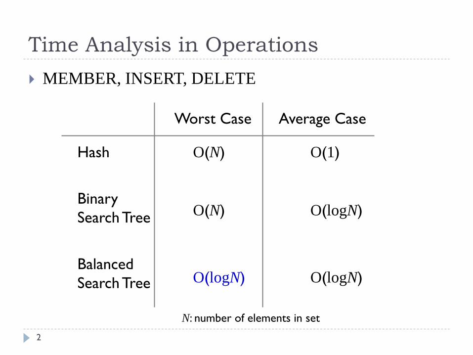
MEMBER, INSERT, DELETE
Hash
Binary
Search Tree
Balanced
Search Tree
Worst Case Average Case
O(N) O(1)
O(N) O(logN)
O(logN) O(logN)
N: number of elements in set
2-3 Tree
3
Balanced Tree – 2-3 tree
4
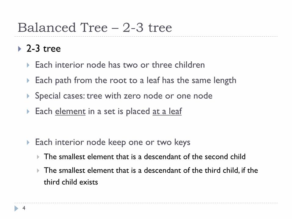
2-3 tree
Each interior node has two or three children
Each path from the root to a leaf has the same length
Special cases: tree with zero node or one node
Each element in a set is placed at a leaf
Each interior node keep one or two keys
The smallest element that is a descendant of the second child
The smallest element that is a descendant of the third child, if the
third child exists
Balanced Tree – 2-3 tree
5
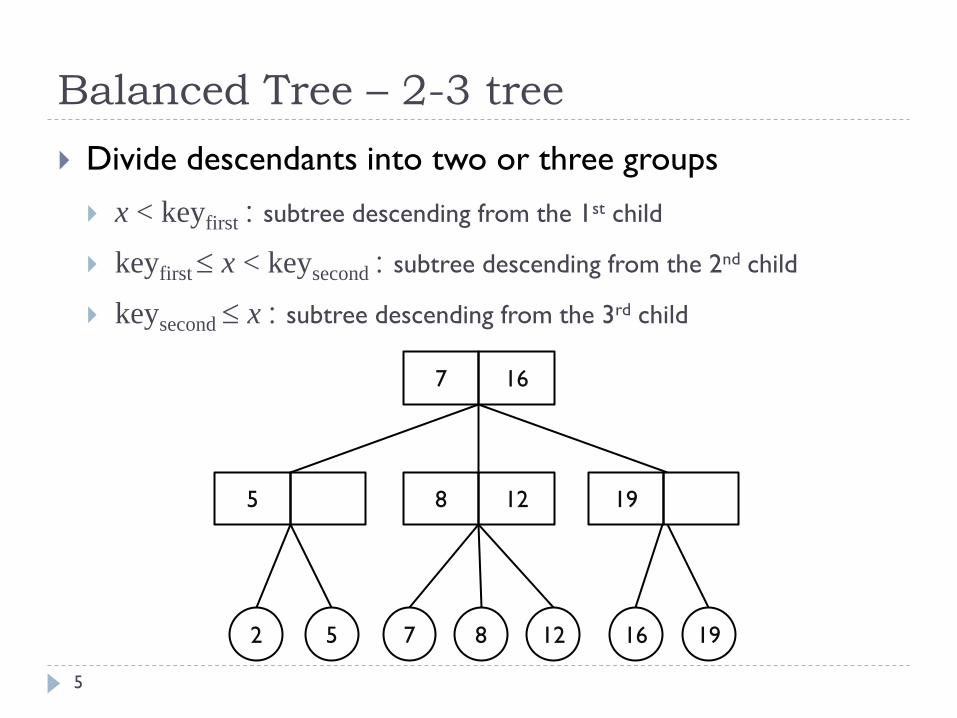
Divide descendants into two or three groups
x < keyfirst : subtree descending from the 1st child
keyfirst x < keysecond : subtree descending from the 2nd child
keysecond x : subtree descending from the 3rd child
7 16
5 8 12 19
2 5 16 19 7 8 12
2-3 Tree – operations
6
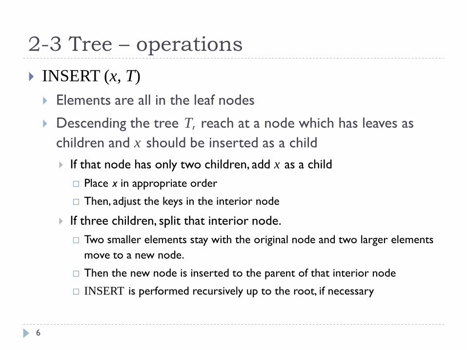
INSERT (x, T)
Elements are all in the leaf nodes
Descending the tree T, reach at a node which has leaves as
children and x should be inserted as a child
If that node has only two children, add x as a child
Place x in appropriate order
Then, adjust the keys in the interior node
If three children, split that interior node.
Two smaller elements stay with the original node and two larger elements
move to a new node.
Then the new node is inserted to the parent of that interior node
INSERT is performed recursively up to the root, if necessary
2-3 Tree - operations
7
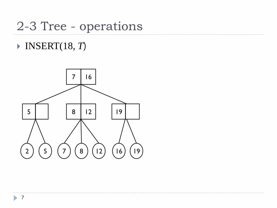
INSERT(18, T)
7 16
5 8 12 19
2 5 16 19 7 8 12
2-3 Tree - operations
8
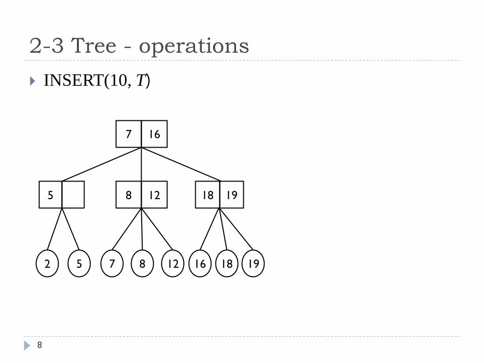
INSERT(10, T)
7 16
5 8 12 18 19
2 5 16 19 7 8 12 18
2-3 Tree - operations
9
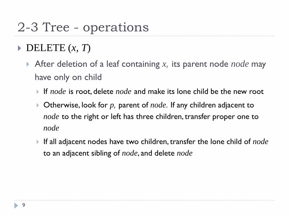
DELETE (x, T)
After deletion of a leaf containing x, its parent node node may
have only on child
If node is root, delete node and make its lone child be the new root
Otherwise, look for p, parent of node. If any children adjacent to
node to the right or left has three children, transfer proper one to
node
If all adjacent nodes have two children, transfer the lone child of node
to an adjacent sibling of node, and delete node

2-3 Tree - operations
10
DELETE (10, T)
7
5 8 18 19
2 5 16 19 7 8 18
12
10 12
16
10

2-3 Tree - operations
11
DELETE (7, T)
7
5 8 19
2 5 19 7 8 18
16
12 16
18
12
2-3 Tree - operations
12
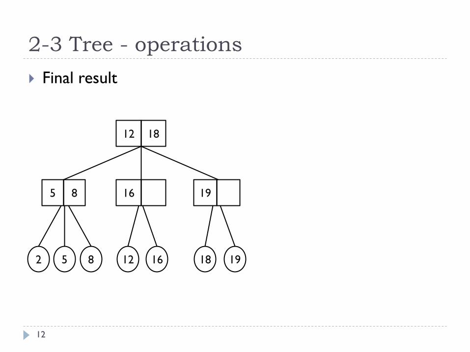
Final result
12 18
5 8 16 19
2 5 16 19 8 12 18
B-Tree
13
B-Tree
14
Balanced search tree
Height = O(logN) for the worst case
Keys are stored in internal nodes and leaves
Designed to work well on storage devices (e.g. disk)
Show good performance on disk I/O operations
Widely used in database systems
Variants
B+Tree : keys and records are stored in leaves
Copies of keys are stored in internal nodes
Leaves are linked in a list for a fast sequential search
B*Tree: dense node (at least 2/3 full, instead ½ full)
B-Tree: Motivation
15
Data structures on secondary storage
Main memory is fast but expensive
Magnetic disks are cheaper and high capacity, but slow
B-trees try to read as much information as possible in
every disk access operation

B-Tree: Definition
16
B-tree T is a rooted tree (with root root[T])
Every node x has following fields
n[x]: number of keys currently stored in node x
keys: n[x] keys stored in non-decreasing order
key1[x] ≤ key2[x] ≤ … ≤ keyn[x][x]
leaf[x]: a boolean value – true if x is a leaf, false if x is an internal node
child pointers: c1[x], c2[x], …, cn[x]+1[x], if x is an internal node
key1 key2 keyn[x] …
c1 c2 c3 cn[x] cn[x]+1

B-Tree: Definition (cont’d)
17
Properties (cont’d)
keys keyi[x] separate the ranges of keys stored in each subtree:
if ki is any key stored in a subtree with root ci[x], then
k1 ≤ key1[x] ≤ k2 ≤ key2[x] ≤ … ≤ keyn[x][x] ≤ kn[x]+1
all leaves have the same height, which is the tree’s height h
upper & lower bounds on the number of keys on a node
minimum degree of B-tree: t (a fixed integer t ≥ 2)
lower bound: at least t-1 keys (at least t children), except root
upper bound: at most 2t-1 keys (at most 2t children)
Height of B-Tree
18
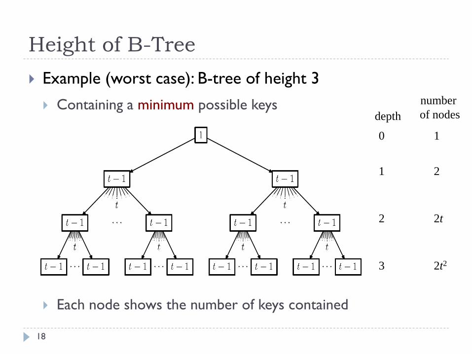
Example (worst case): B-tree of height 3
Containing a minimum possible keys
Each node shows the number of keys contained
depth
number
of nodes
0
1
2
3
1
2
2t
2t2
Height of B-Tree (cont’d)
19
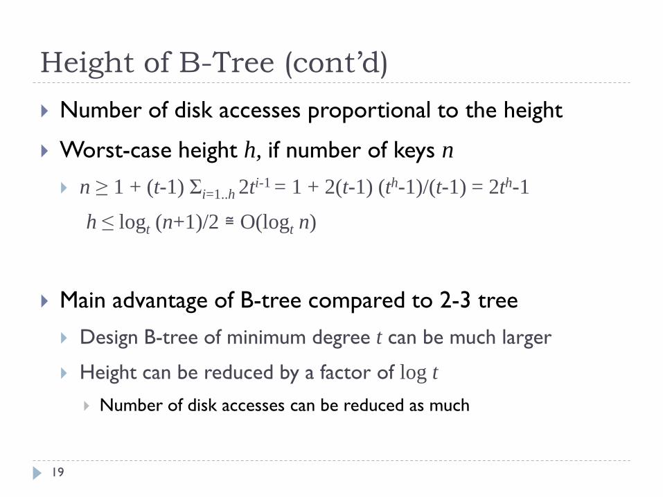
Number of disk accesses proportional to the height
Worst-case height h, if number of keys n
n ≥ 1 + (t-1) Σi=1..h 2ti-1 = 1 + 2(t-1) (th-1)/(t-1) = 2th-1
h ≤ logt (n+1)/2 ≅ O(logt n)
Main advantage of B-tree compared to 2-3 tree
Design B-tree of minimum degree t can be much larger
Height can be reduced by a factor of log t
Number of disk accesses can be reduced as much
Basic Operations on B-Tree
20
Operations
SEARCH (MEMBER)
INSERT
DELETE
Algorithms
Root of B-tree is always in main memory
DISK-READ of a node along the path downward the B-tree
B-Tree Search
21
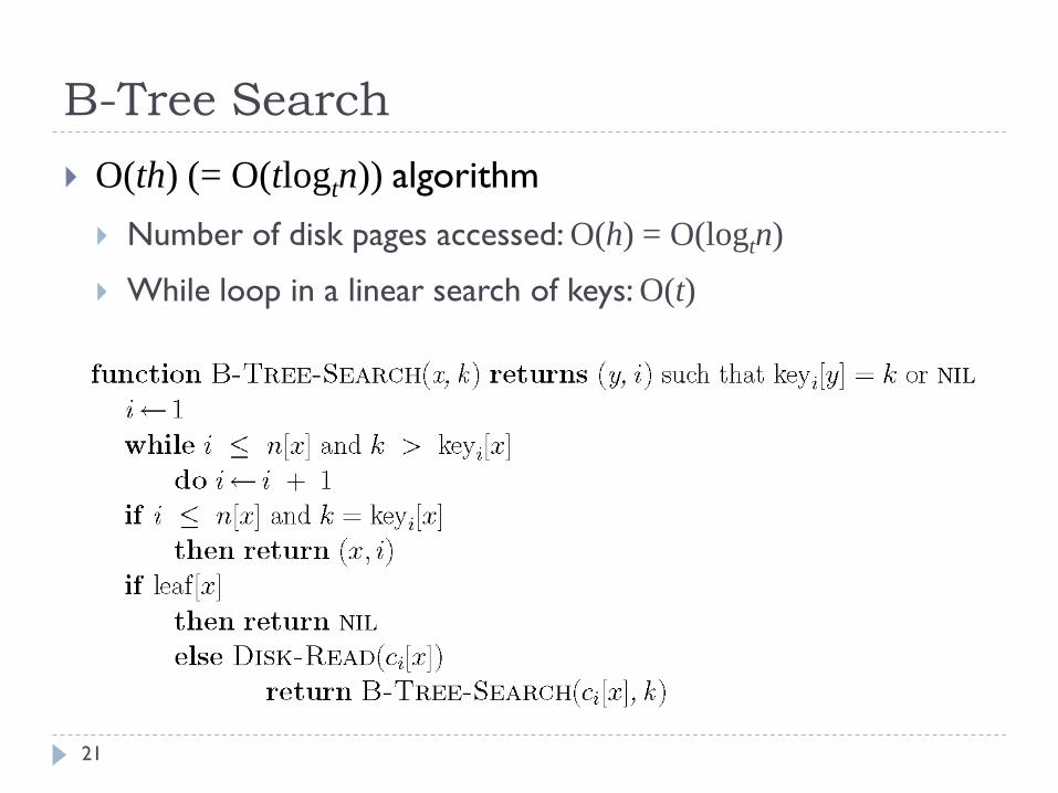
O(th) (= O(tlogtn)) algorithm
Number of disk pages accessed: O(h) = O(logtn)
While loop in a linear search of keys: O(t)
B-Tree Insert
22
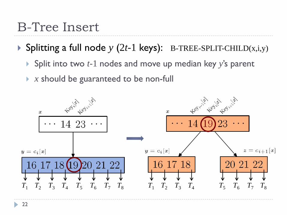
Splitting a full node y (2t-1 keys): B-TREE-SPLIT-CHILD(x,i,y)
Split into two t-1 nodes and move up median key y’s parent
x should be guaranteed to be non-full
T1 T2 T3 T4 T5 T6 T7 T8 T1 T2 T3 T4 T5 T6 T7 T8
B-Tree Insert
23
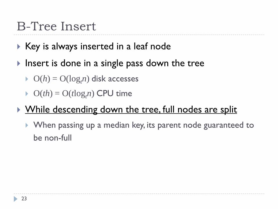
Key is always inserted in a leaf node
Insert is done in a single pass down the tree
O(h) = O(logtn) disk accesses
O(th) = O(tlogtn) CPU time
While descending down the tree, full nodes are split
When passing up a median key, its parent node guaranteed to
be non-full
B-Tree Insert – Example (I)
24
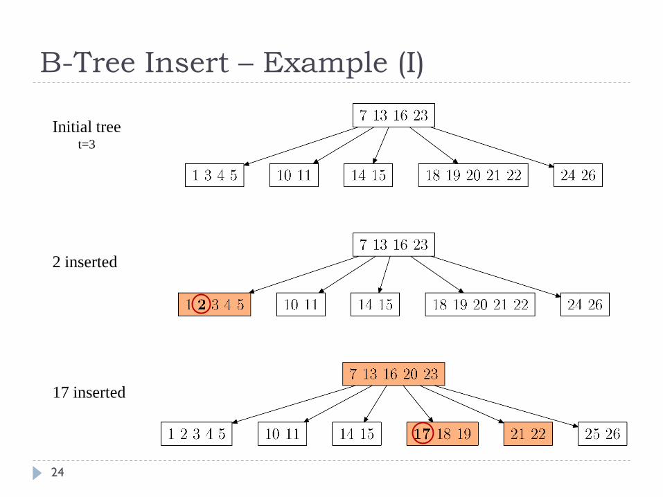
Initial tree t=3
2 inserted
17 inserted

B-Tree Insert – Example (II)
25
Initial tree t=3
12 inserted
6 inserted
B-Tree Delete
26
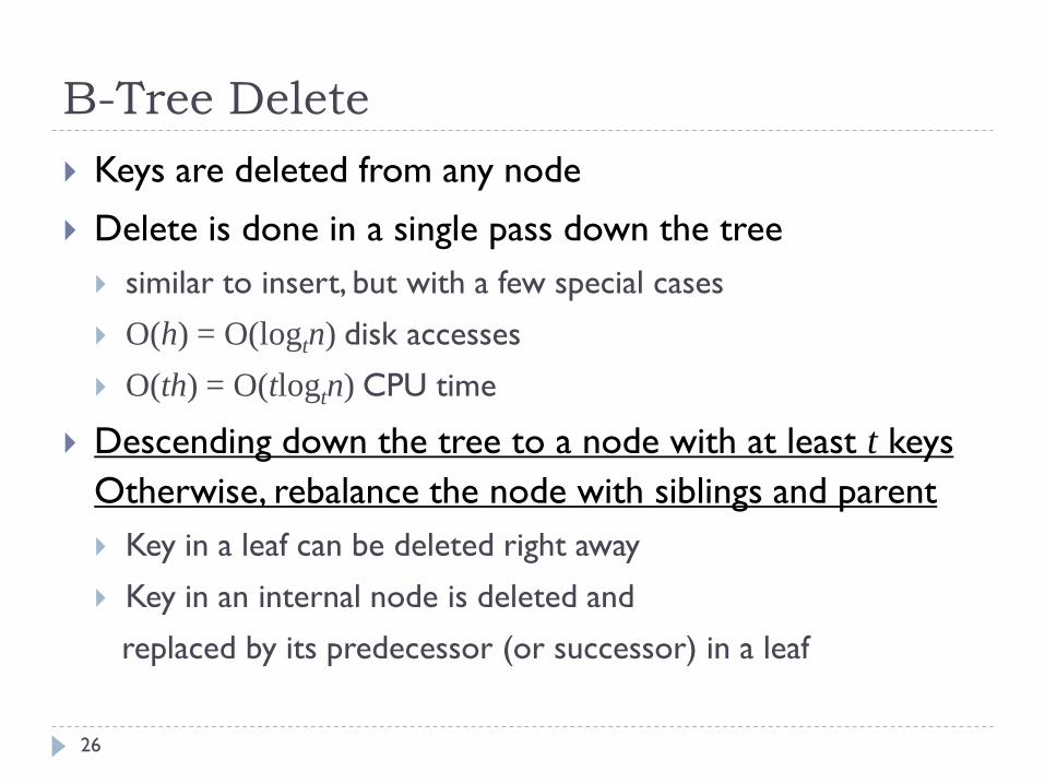
Keys are deleted from any node
Delete is done in a single pass down the tree
similar to insert, but with a few special cases
O(h) = O(logtn) disk accesses
O(th) = O(tlogtn) CPU time
Descending down the tree to a node with at least t keys
Otherwise, rebalance the node with siblings and parent
Key in a leaf can be deleted right away
Key in an internal node is deleted and
replaced by its predecessor (or successor) in a leaf
B-Tree Delete
27
k: the key to be deleted, x: the node containing the key
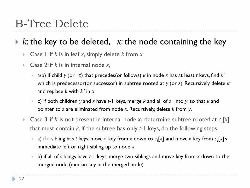
Case 1: if k is in leaf x, simply delete k from x
Case 2: if k is in internal node x,
a/b) if child y (or z) that precedes(or follows) k in node x has at least t keys, find k’
which is predecessor(or successor) in subtree rooted at y (or z). Recursively delete k’
and replace k with k’ in x
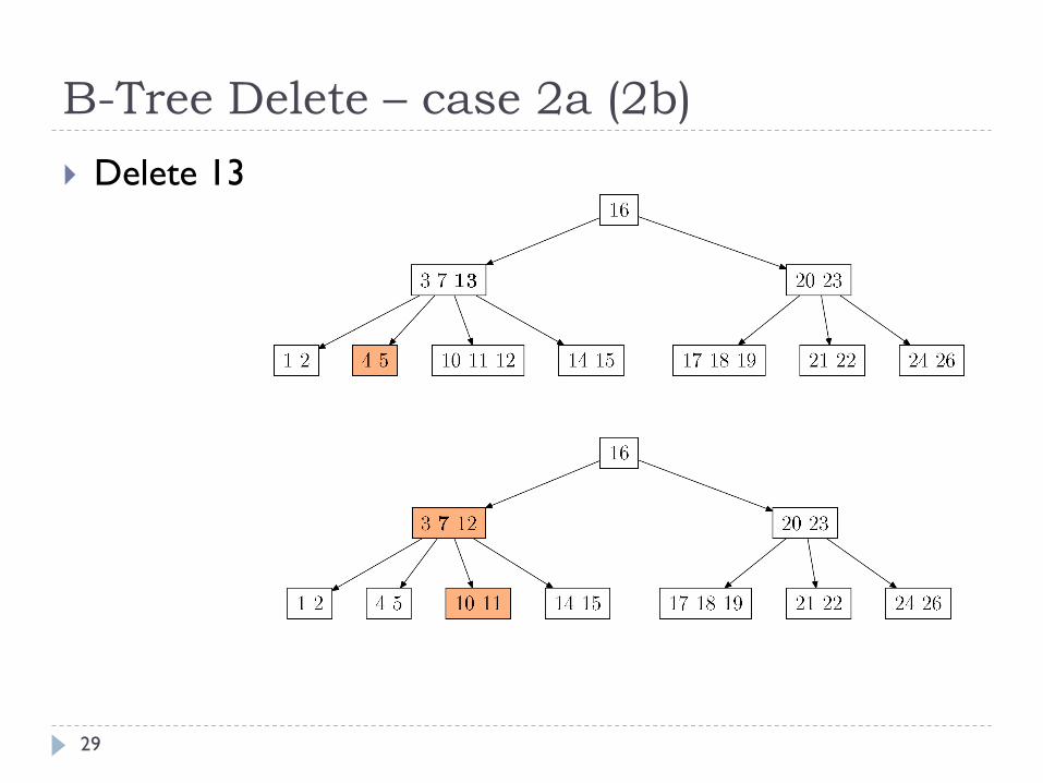
c) if both children y and z have t-1 keys, merge k and all of z into y, so that k and
pointer to z are eliminated from node x. Recursively, delete k from y.
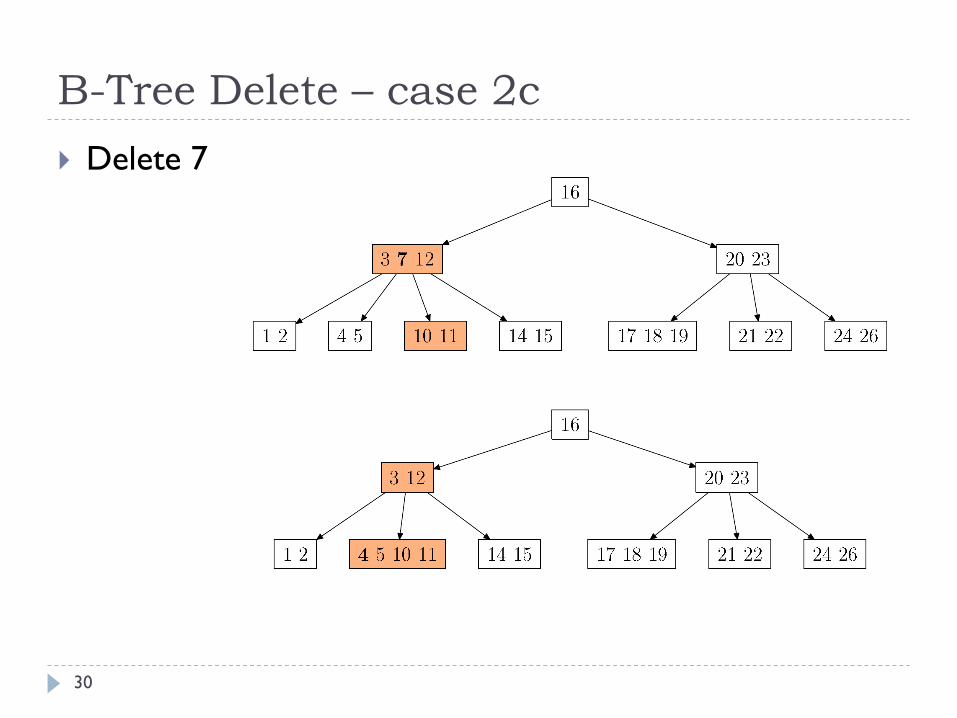
Case 3: if k is not present in internal node x, determine subtree rooted at ci[x]
that must contain k. If the subtree has only t-1 keys, do the following steps
a) if a sibling has t keys, move a key from x down to ci[x] and move a key from ci[x]’s
immediate left or right sibling up to node x
b) if all of siblings have t-1 keys, merge two siblings and move key from x down to the
merged node (median key in the merged node)

B-Tree Delete – case 1
28
Delete 6
B-Tree Delete – case 2a (2b)
29
Delete 13
B-Tree Delete – case 2c
30
Delete 7

B-Tree Delete – case 3b
31
Delete 4
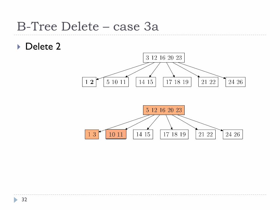
B-Tree Delete – case 3a
32
Delete 2
10 11

Hwansoo Han (SKKU)
Skip List
‣ Examples
‣ Treaps
‣ B-tree
‣ skip list
‣ Dynamic
‣ insert, delete, search
‣ Fast operation - O(log N)
‣ O(log N) with a high probability
Dynamic Search Structures
2
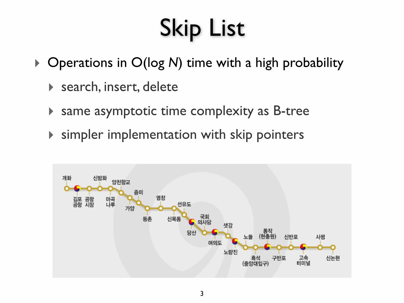
‣ Operations in O(log N) time with a high probability
‣ search, insert, delete
‣ same asymptotic time complexity as B-tree
‣ simpler implementation with skip pointers
Skip List
3
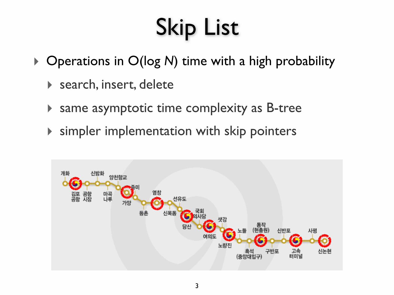
‣ Operations in O(log N) time with a high probability
‣ search, insert, delete
‣ same asymptotic time complexity as B-tree
‣ simpler implementation with skip pointers
Skip List
3

‣ Skipping along the express lane
‣ Skipping every other node
‣ additional memory usage: N/2
‣ search time: ⎡N/2⎤ + 1 (at max)
“Express Lane”
4
1 2 3 4 5 6 7 8 9 10 header

‣ Add another express lane
‣ Skipping 3 nodes and link the 4th node
‣ additional memory usage: 3/4 × N ( = N/2 + N/4)
‣ search time: ⎡N/4⎤ + 2 (at max)
Another “Express Lane”
5
1 2 3 4 5 6 7 8 9 10 header

‣ Add more “express lanes” by doubling the distance
‣ Every (2i)th node has a pointer to 2i ahead
‣ 50% nodes belong to 2 pointer lists,
‣ 25% nodes belong to 3 pointer lists,
‣ 12.5% nodes belong to 4 pointer lists, ...
Generalized “Express Lanes”
6
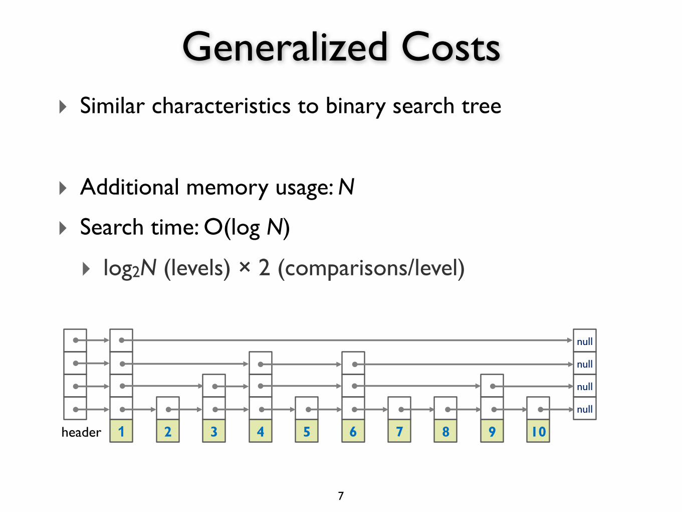
‣ Similar characteristics to binary search tree
‣ Additional memory usage: N
‣ Search time: O(log N)
‣ log2N (levels) × 2 (comparisons/level)
Generalized Costs
7
1 2 3 4 5 6 7 8 9 10
null
null
null
null
header
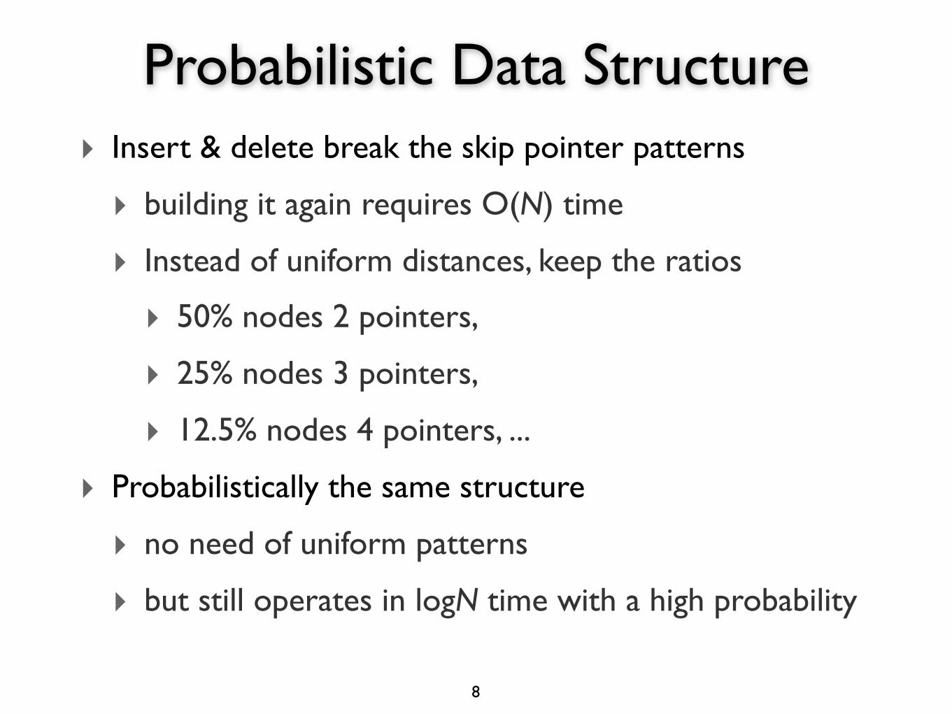
‣ Insert & delete break the skip pointer patterns
‣ building it again requires O(N) time
‣ Instead of uniform distances, keep the ratios
‣ 50% nodes 2 pointers,
‣ 25% nodes 3 pointers,
‣ 12.5% nodes 4 pointers, ...
‣ Probabilistically the same structure
‣ no need of uniform patterns
‣ but still operates in logN time with a high probability
Probabilistic Data Structure
8
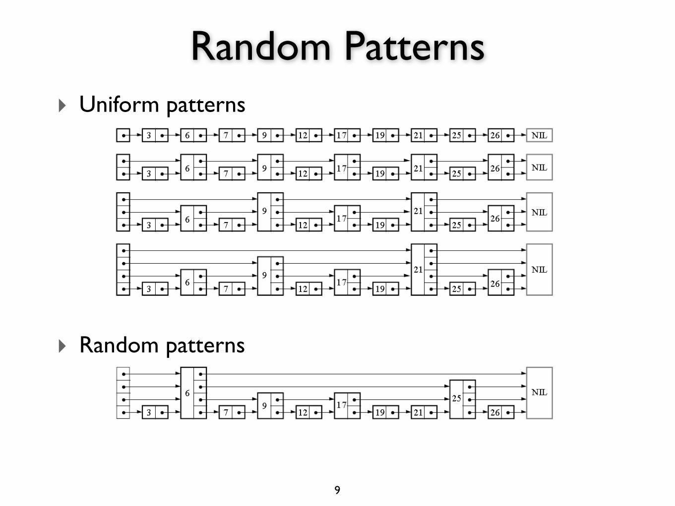
‣ Uniform patterns
‣ Random patterns
Random Patterns
9

‣ Fraction p of the nodes with level i pointers also have level i+1 pointers
‣ p = 1/2 (original discussion)
‣ p can be 1/4 for performance and memory usage
‣ Maximum number of pointers at level 1: log1/p N
‣ Most implementation fixes the max number to 20
‣ Number of levels: log1/p N
‣ Search time: O(log N) = (log1/p N) × 1/p
Fraction p
10
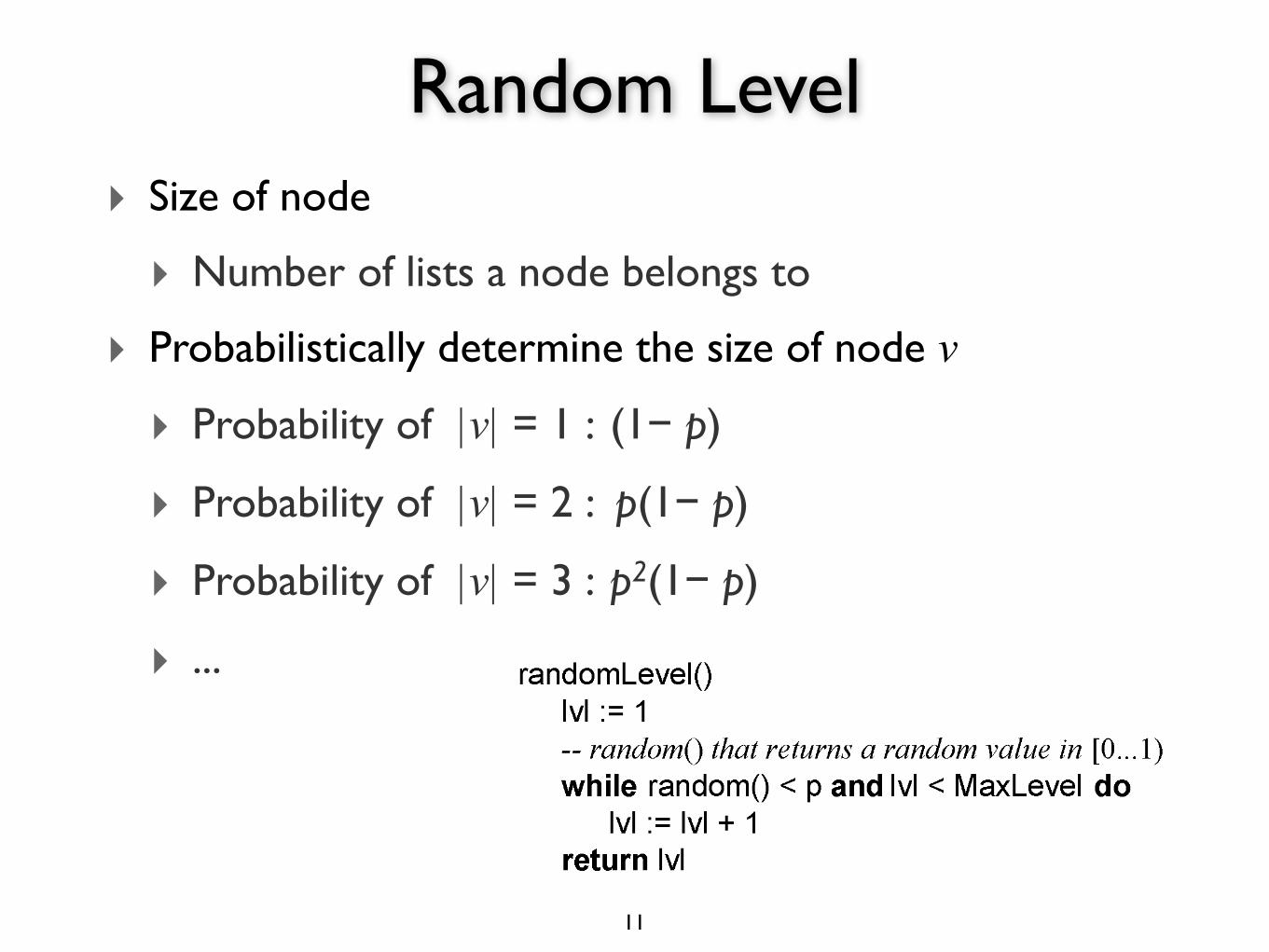
‣ Size of node
‣ Number of lists a node belongs to
‣ Probabilistically determine the size of node v
‣ Probability of |v| = 1 : (1− p)
‣ Probability of |v| = 2 : p(1− p)
‣ Probability of |v| = 3 : p2(1− p)
‣ ...
Random Level
11
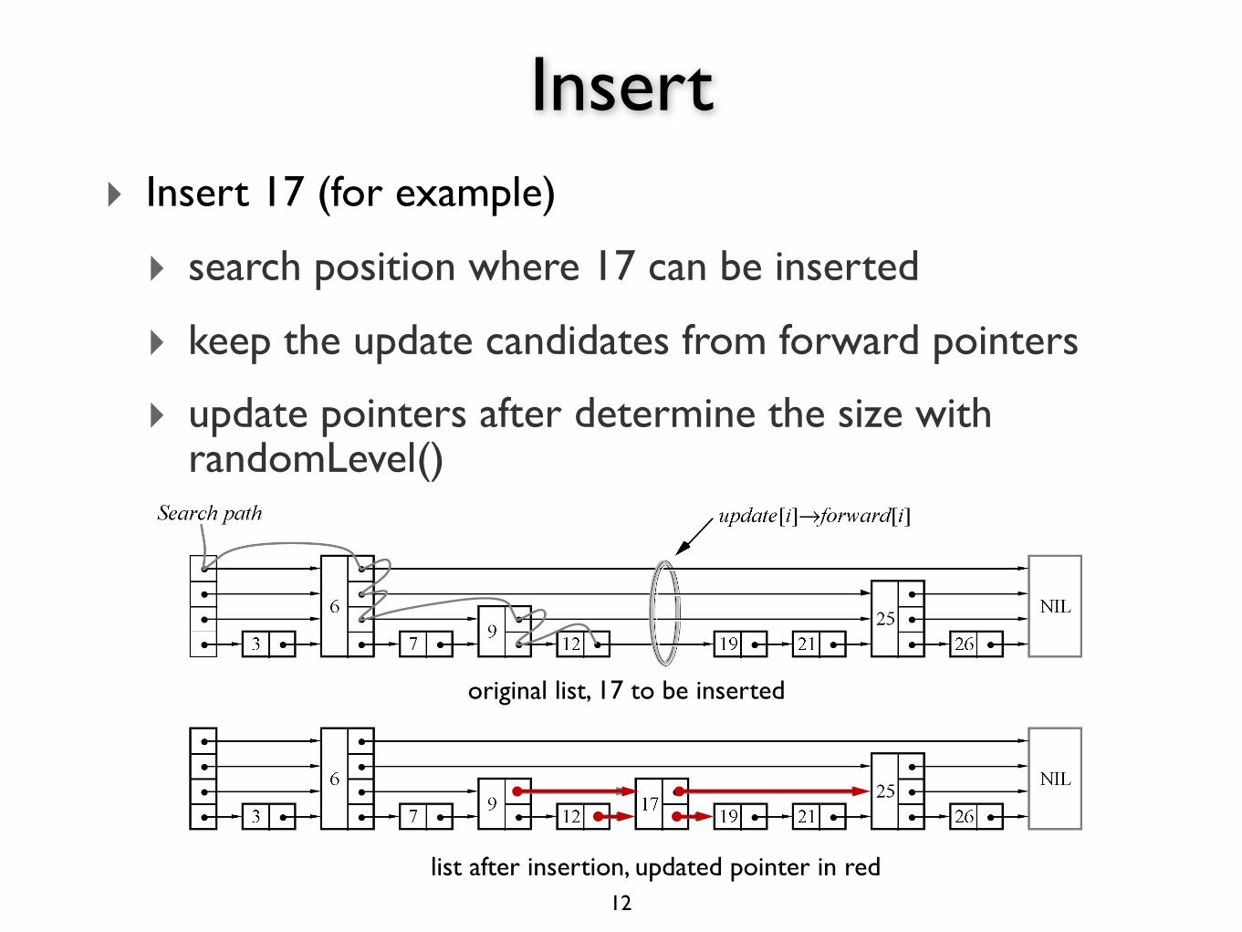
‣ Insert 17 (for example)
‣ search position where 17 can be inserted
‣ keep the update candidates from forward pointers
‣ update pointers after determine the size with randomLevel()
Insert
12
list after insertion, updated pointer in red
original list, 17 to be inserted
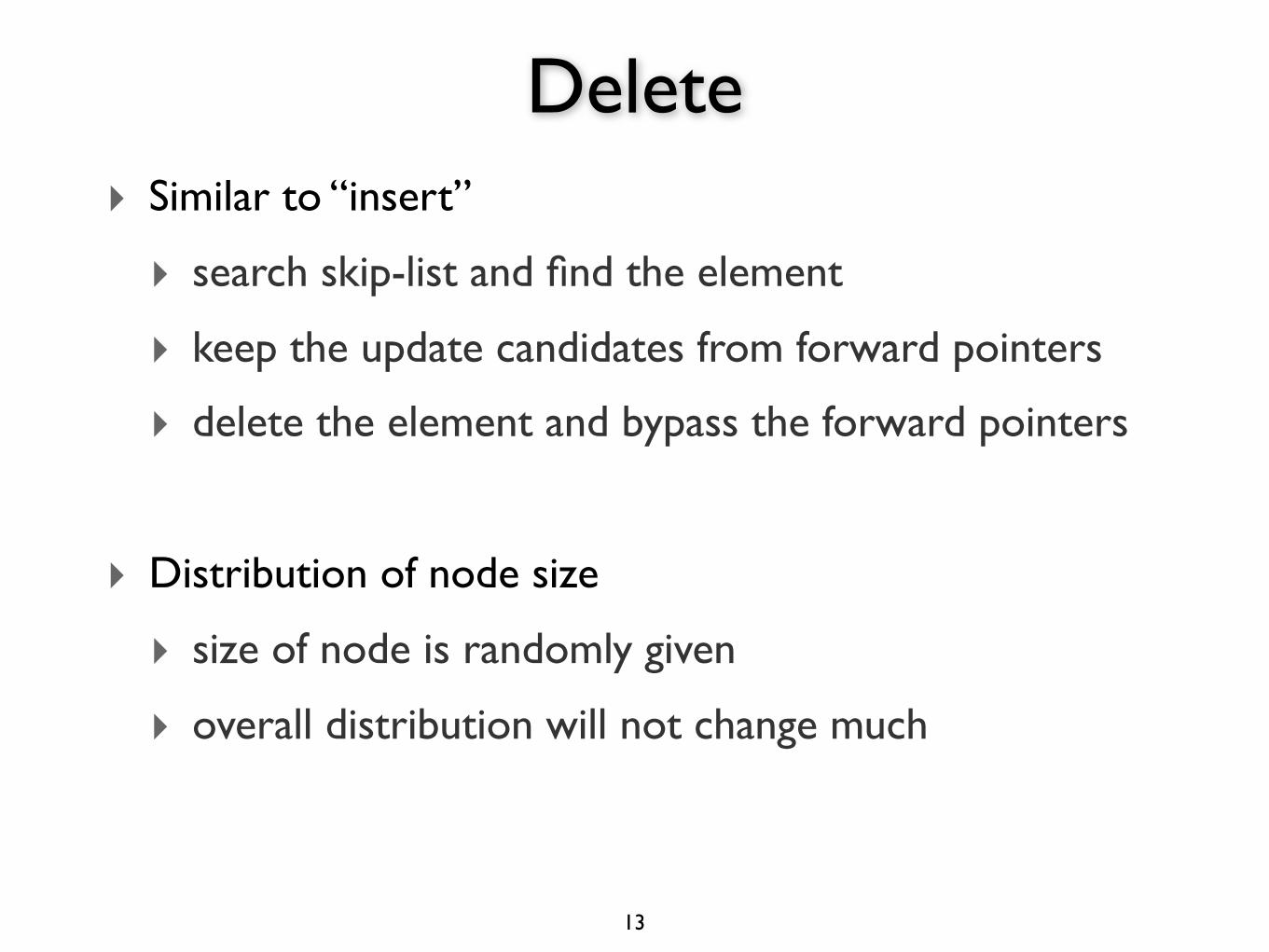
‣ Similar to “insert”
‣ search skip-list and find the element
‣ keep the update candidates from forward pointers
‣ delete the element and bypass the forward pointers
‣ Distribution of node size
‣ size of node is randomly given
‣ overall distribution will not change much
Delete
13
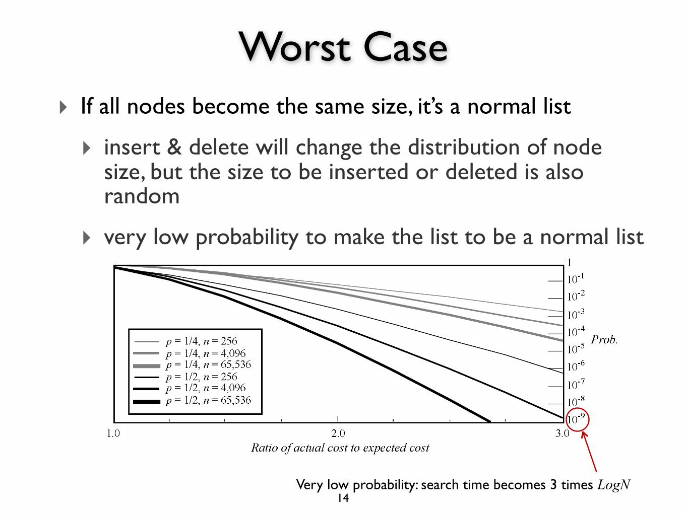
‣ If all nodes become the same size, it’s a normal list
‣ insert & delete will change the distribution of node size, but the size to be inserted or deleted is also random
‣ very low probability to make the list to be a normal list
Worst Case
14Very low probability: search time becomes 3 times LogN
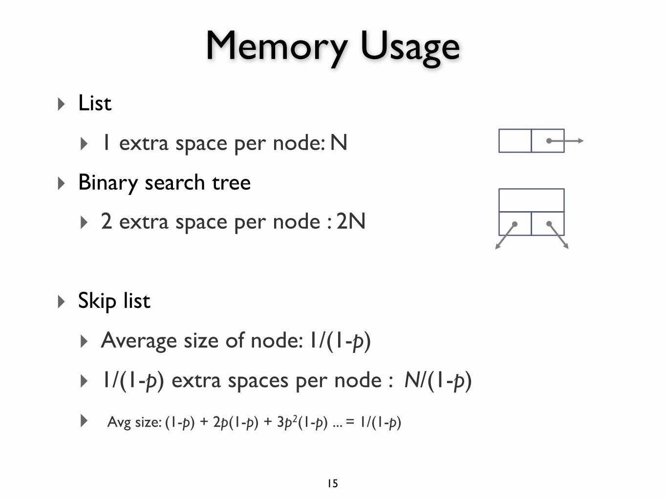
‣ List
‣ 1 extra space per node: N
‣ Binary search tree
‣ 2 extra space per node : 2N
‣ Skip list
‣ Average size of node: 1/(1-p)
‣ 1/(1-p) extra spaces per node : N/(1-p)
‣ Avg size: (1-p) + 2p(1-p) + 3p2(1-p) ... = 1/(1-p)
Memory Usage
15
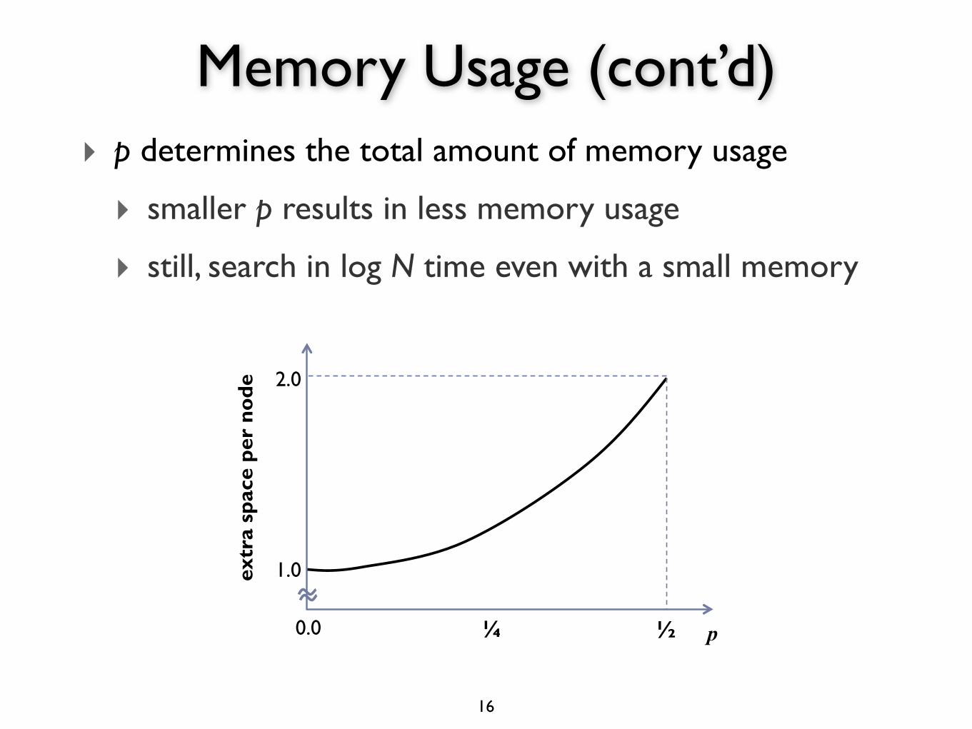
‣ p determines the total amount of memory usage
‣ smaller p results in less memory usage
‣ still, search in log N time even with a small memory
Memory Usage (cont’d)
16
2.0
1.0
0.0 ½
extr
a sp
ace
per
node
p ¼
‣ Useful in parallel computing
‣ concurrent insert in different parts
‣ no need of global rebalancing
‣ Resource discovery in ad-hoc wireless network
‣ Skip Graphs - robust to the loss of any single node
‣ Sometimes, skip list performs worse than B-tree
‣ due to memory locality, and
‣ more space requirement (from fragmentation)
Skip List Usage
17
‣ Redis (BSD)
‣ open source persistent key/value store for Posix systems
‣ Qmap (GPL, LGPL)
‣ template class of Qt which provides a dictionary type
‣ Skipdb (BSD)
‣ open source database format using ordered key/value pairs
‣ ConcurrentSkipListSet, ConcurrentSkipListMap in Java 1.6
‣ concurrent version of Set and Map using skip list
Skip List Adoption
18