Session 4: Visualization and GUIprogramming Version 1.0.2

Aaron Ponti

Contents

1 Visualization 11.1 A MATLAB graph . . . . . . . . . . . . . . . . . . . . . . . . . . . 11.2 Figure toolbars . . . . . . . . . . . . . . . . . . . . . . . . . . . . . 31.3 Types of plots . . . . . . . . . . . . . . . . . . . . . . . . . . . . . 4

1.3.1 Two-dimensional plotting functions . . . . . . . . . . . . 41.3.2 Three-dimensional plotting functions . . . . . . . . . . . 5

1.4 Interactive plots with the plot tools . . . . . . . . . . . . . . . . . 61.5 Basic plotting commands . . . . . . . . . . . . . . . . . . . . . . . 7

1.5.1 Creating Figure Windows . . . . . . . . . . . . . . . . . . 71.5.2 Displaying Multiple Plots per Figure . . . . . . . . . . . . 81.5.3 Specifying the Target Axes . . . . . . . . . . . . . . . . . 8

1.6 Using High-Level Plotting Functions . . . . . . . . . . . . . . . 91.6.1 Functions for Plotting Line Graphs . . . . . . . . . . . . 91.6.2 Programmatic plotting . . . . . . . . . . . . . . . . . . . . 91.6.3 Creating line plots . . . . . . . . . . . . . . . . . . . . . . 101.6.4 Specifying line style . . . . . . . . . . . . . . . . . . . . . 121.6.5 Colors, line styles, and markers . . . . . . . . . . . . . . . 131.6.6 Specifying the Color and Size of Lines . . . . . . . . . . 141.6.7 Adding Plots to an Existing Graph . . . . . . . . . . . . 141.6.8 Line Plots of Matrix Data . . . . . . . . . . . . . . . . . . 151.6.9 Plotting with two y-axes . . . . . . . . . . . . . . . . . . . 171.6.10 Combining linear and logarithmic axes . . . . . . . . . . 17

1.7 Setting axis parameters . . . . . . . . . . . . . . . . . . . . . . . . 181.7.1 Axis Scaling and Ticks . . . . . . . . . . . . . . . . . . . . 181.7.2 Axis Limits and Ticks . . . . . . . . . . . . . . . . . . . . 191.7.3 Semiautomatic Limits . . . . . . . . . . . . . . . . . . . . 191.7.4 Axis tick marks . . . . . . . . . . . . . . . . . . . . . . . . 191.7.5 Example — Specifying Ticks and Tick Labels . . . . . . . 191.7.6 Setting aspect ratio . . . . . . . . . . . . . . . . . . . . . . 20

1.8 Printing and exporting . . . . . . . . . . . . . . . . . . . . . . . . 211.8.1 Graphical user interfaces . . . . . . . . . . . . . . . . . . 221.8.2 Command line interface . . . . . . . . . . . . . . . . . . . 27

1.9 References . . . . . . . . . . . . . . . . . . . . . . . . . . . . . . . 28

1

2 Creating Graphical User Interfaces 282.1 What is a GUI? . . . . . . . . . . . . . . . . . . . . . . . . . . . . . 282.2 Ways to build MATLAB GUIs . . . . . . . . . . . . . . . . . . . . 292.3 Creating a simple GUI with GUIDE . . . . . . . . . . . . . . . . 30

2.3.1 Laying out the GUI with GUIDE . . . . . . . . . . . . . . 302.3.2 Adding code to the GUI . . . . . . . . . . . . . . . . . . . 38

2.4 Creating a simple GUI programmatically . . . . . . . . . . . . . 412.4.1 Creating a GUI code file . . . . . . . . . . . . . . . . . . . 412.4.2 Laying out a simple GUI . . . . . . . . . . . . . . . . . . . 42

2.5 References . . . . . . . . . . . . . . . . . . . . . . . . . . . . . . . 47

1 Visualization

1.1 A MATLAB graph

The MATLAB environment offers a variety of data plotting functions plus a setof Graphical User Interface (GUI) tools to create, and modify graphic displays.

A figure is a MATLAB window that contains graphic displays (usually dataplots) and UI components. You create figures explicitly with the figure function,and implicitly whenever you plot graphics and no figure is active.

h = figure;

By default, figure windows are resizable and include pull-down menus andtoolbars.

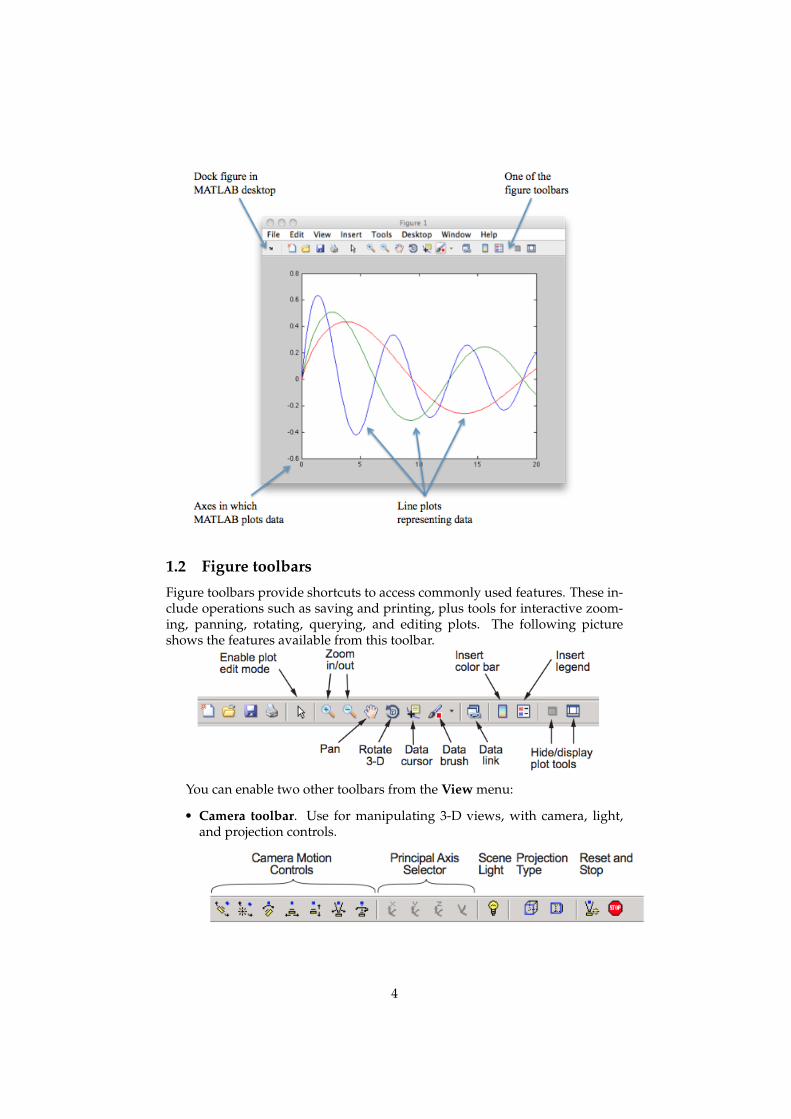
A plot is any graphic display you can create within a figure window. Plotscan display tabular data, geometric objects, surface and image objects, and an-notations such as titles, legends, and colorbars. Figures can contain any num-ber of plots. Each plot is created within a 2-D or a 3-D data space called an axes.You can explicitly create axes with the axes or subplot functions.

A graph is a plot of data within a 2-D or 3-D axes. Most plots made withMATLAB functions and GUIs are therefore graphs. When you graph a one-dimensional variable (e.g., rand(100,1)), the indices of the data vector (in thiscase 1:100) become assigned as x values, and plots the data vector as y values.Some types of graphs can display more than one variable at a time, otherscannot.

x = 0:.2:20;y = sin(x)./sqrt(x+1);y(2,:) = sin(x/2)./sqrt(x+1);y(3,:) = sin(x/3)./sqrt(x+1);plot(x,y)

2

The resulting figure contains a 2-D set of axes.The plot function uses a default line style and color to distinguish the data

sets plotted in the graph. You can change the appearance of these graphic com-ponents or add annotations to the graph to present your data in a particularway.

This graphic identifies the components and tools of a figure window.

3

1.2 Figure toolbars

Figure toolbars provide shortcuts to access commonly used features. These in-clude operations such as saving and printing, plus tools for interactive zoom-ing, panning, rotating, querying, and editing plots. The following pictureshows the features available from this toolbar.

You can enable two other toolbars from the View menu:

• Camera toolbar. Use for manipulating 3-D views, with camera, light,and projection controls.

4

• Plot Edit toolbar. Use for annotation and setting plot and object proper-ties.

1.3 Types of plots

You can construct a wide variety of 2-D and 3-D MATLAB plots with very little,if any, programming required on your part. The following two tables classifyand illustrate most of the kinds of plots you can create. They include line, bar,area, direction and vector field, radial, and scatter graphs. They also include 2-D and 3-D functions that generate and plot geometric shapes and objects. Most2-D plots have 3-D analogs, and there are a variety of volumetric displays for3-D solids and vector fields. Plot types that begin with “ez” (such as ezsurf ) areconvenience functions that can plot arguments given as functions.

1.3.1 Two-dimensional plotting functions

The table below shows all available MATLAB 2-D plot functions. You can getdocumentation for each of the functions by typing help function_name in theMATLAB console, for example:

help plotyy

5

1.3.2 Three-dimensional plotting functions

The table below shows all available MATLAB 3-D and volumetric plot func-tions. It includes functions that generate 3-D data (cylinder, ellipsoid, sphere),but most plot either arrays of data or functions.

6

1.4 Interactive plots with the plot tools

Most of the plotting functions shown in the previous tables are accessible throughthe Figure Palette, one of the Plot Tools you can access via the figure windowView menu. When the Figure Palette is active and you select one, two or morevariables listed within it, you can generate a plot of any appropriate type byright-clicking and selecting a plot type from the context menu that appears.The lowest item on that menu is More Plots. When you select More Plots, thePlot Catalog opens for you to browse through all plot types and generate oneof them, either to display the variables you selected in the Figure Palette or aMATLAB expression you can specify in the Plot Catalog window.

7

We won’t discuss the plot tools in this course.

1.5 Basic plotting commands

1.5.1 Creating Figure Windows

MATLAB graphics are directed to a window that is separate from the Com-mand Window. This window is referred to as a figure. The characteristics ofthis window are controlled by your computer’s windowing system and MAT-LAB figure properties.

Graphics functions automatically create new MATLAB figure windows ifnone currently exist. If a figure already exists, that window is used. If multiplefigures exist, one is designated as the current figure and is used (this is gener-ally the last figure used or the last figure you clicked the mouse in). The figurefunction creates figure windows. For example,

figure

creates a new window and makes it the current figure. You can make an exist-ing figure current by clicking it with the mouse or by passing its handle (thenumber indicated in the window title bar), as an argument to figure.

figure(2)

The handle is returned when the figure is created.

h = figureh =

3

8

1.5.2 Displaying Multiple Plots per Figure

You can display multiple plots in the same figure window and print them onthe same piece of paper with the subplot function. subplot(m,n,i) breaks the fig-ure window into an m-by-n matrix of small subplots and selects the ith subplotfor the current plot. The plots are numbered along the top row of the figurewindow, then the second row, and so forth. For example, the following state-ments plot data in four different subregions of the figure window.

t = 0:pi/20:2*pi;[x,y] = meshgrid(t);subplot(2,2,1); plot(sin(t),cos(t)); axis equal;subplot(2,2,2); z = sin(x)+cos(y); plot(t,z); axis([0 2*pi -2 2]);subplot(2,2,3); z = sin(x).*cos(y); plot(t,z); axis([0 2*pi -1 1]);subplot(2,2,4); z = (sin(x).^2)-(cos(y).^2); plot(t,z); axis([0 2*pi -1 1]);

Each subregion contains its own axes with characteristics you can controlindependently of the other subregions. This example uses the axis function toset limits and change the shape of the subplots. See the axes, axis, and subplotfunctions for more information.

1.5.3 Specifying the Target Axes

The current axes is the last one defined by subplot. If you want to access apreviously defined subplot, for example to add a title, you must first make thataxes current. You can make an axes current in three ways:

9

• Click on the subplot with the mouse.

• Call subplot with the m, n, i specifiers.

subplot(2,2,2); title(’Top Right Plot’);

• Call subplot with the handle (identifier) of the axes.

h = get(gcf,’Children’);subplot(h(1)); title(’Most recently created axes’);subplot(gca); title(’Current active axes’);

The call

get(gcf,’Children’);

returns the handles of all the axes, with the most recently created one first. Thefunction gca returns the handle of the current active axes.

1.6 Using High-Level Plotting Functions

1.6.1 Functions for Plotting Line Graphs

Many types of MATLAB functions are available for displaying vector data asline plots, as well as functions for annotating and printing these graphs. Thefollowing table summarizes the functions that produce basic line plots. Thesefunctions differ in the way they scale the plot’s axes. Each accepts input in theform of vectors or matrices and automatically scales the axes to accommodatethe data.

Function Descriptionplot Graph 2-D data with linear scales for both axesplot3 Graph 3-D data with linear scales for both axesloglog Graph with logarithmic scales for both axes

semilogx Graph with a logarithmic scale for the x-axis and a linear scale for the y-axissemilogy Graph with a logarithmic scale for the y-axis and a linear scale for the x-axis

plotyy Graph with y-tick labels on the left and right side

1.6.2 Programmatic plotting

The process of constructing a basic graph to meet your presentation graphicsrequirements is outlined in the following table. The table shows seven typicalsteps and some example code for each. If you are performing analysis only, youmay want to view various graphs just to explore your data. In this case, steps 1and 3 may be all you need. If you are creating presentation graphics, you maywant to fine-tune your graph by positioning it on the page, setting line stylesand colors, adding annotations, and making other such improvements.

10

Step Typical code1 Prepare your data x = 0:0.2:12;

y1 = besselj(1,x);y2 = besselj(2,x);y3 = besselj(3,x);

2 Select a window and positiona plot region within thewindow

figure(1);subplot(2,2,1);

3 Call elementary plottingfunction

h = plot(x,y1,x,y2,x,y3);

4 Select line and markercharacteristics

set(h,’LineWidth’,2, ...{’LineStyle’},{’–’;’:’;’-.’});set(h,{’Marker’},{’none’;’o’;’x’ });set(h,{’Color’},{’r’;’g’;’b’});

5 Set axis limits, tick marks, andgrid lines

axis([0 12 -0.5 1]);grid on;

6 Annotate the graph with axislabels, legend, and text

xlabel(’Time’);ylabel(’Amplitude’);legend(h,’First’,’Second’,’Third’);title(’Bessel Functions’);[y,ix] = min(y1);text(x(ix),y,’First Min \rightarrow’, ...’HorizontalAlignment’,’right’);

7 Export graph print -depsc -tiff -r200 myplot

1.6.3 Creating line plots

The plot function has different forms depending on the input arguments. Forexample, if y is a vector, plot(y) produces a linear graph of the elements of yversus the index of the elements of y. If you specify two vectors as arguments,plot(x,y) produces a graph of y versus x. For example, the following statementscreate a vector of values in the range [0, 2π] in increments of π/100 and thenuse this vector to evaluate the sine function over that range. MATLAB plotsthe vector on the x-axis and the value of the sine function on the y-axis.

t = 0:pi/100:2*pi;y = sin(t);plot(t,y);grid on % Turn on grid lines for this plot

11

Appropriate axis ranges and tick mark locations are automatically selected.You can plot multiple graphs in one call to plot using x-y pairs. MATLAB

automatically cycles through a predefined list of colors (determined by the axesColorOrder property) to allow discrimination between sets of data. Plottingthree curves as a function of t produces

y = sin(t);y2 = sin(t-0.25);y3 = sin(t-0.5);plot(t,y,t,y2,t,y3)

12

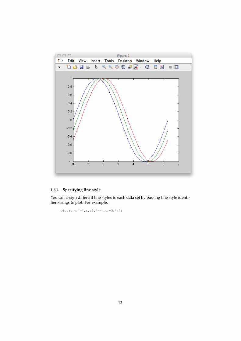
1.6.4 Specifying line style

You can assign different line styles to each data set by passing line style identi-fier strings to plot. For example,

plot(t,y,’-’,t,y2,’--’,t,y3,’:’)

13

The graph shows three lines of different colors and lines styles representingthe value of the sine function with a small phase shift between each line, asdefined by y, y2, and y3. The lines are blue solid, green dashed, and red dotted.

1.6.5 Colors, line styles, and markers

The basic plotting functions accepts character-string arguments that specifyvarious line styles, marker symbols, and colors for each vector plotted. In thegeneral form,

plot(x,y,’linestyle_marker_color’)

linestyle_marker_color is a character string (delineated by single quotation marks)constructed from:

• A line style (e.g., dashed, dotted, etc.)

• A marker type (e.g., x, *, o, etc.)

• A predefined color specifier (c, m, y, k, r, g, b, w)

For example,

plot(x,y,’:squarey’)

14

plots a yellow dotted line and places square markers at each data point. Ifyou specify a marker type, but not a line style, only the marker is plotted.The specification can consist of one or none of each specifier in any order. Forexample, the string

’go--’

defines a dashed line with circular markers, both colored green. You can alsospecify the size of the marker and, for markers that are closed shapes, you canspecify separately the colors of the edges and the face.

1.6.6 Specifying the Color and Size of Lines

You can control a number of line style characteristics by specifying values forline properties:

• LineWidth — Width of the line in units of points

• MarkerEdgeColor — Color of the marker or the edge color for filled mark-ers (circle, square, diamond, pentagram, hexagram, and the four trian-gles)

• MarkerFaceColor — Color of the face of filled markers

• MarkerSize — Size of the marker in units of points

For example, these statements,

x = -pi:pi/10:pi;y = tan(sin(x)) - sin(tan(x));plot(x,y,’--rs’,’LineWidth’,2,...’MarkerEdgeColor’,’k’,...’MarkerFaceColor’,’g’,...’MarkerSize’,10)

produce a graph with:

• A red dashed line with square markers

• A line width of two points

• The edge of the marker colored black

• The face of the marker colored green

• The size of the marker set to 10 points

Try!

1.6.7 Adding Plots to an Existing Graph

You can add plots to an existing graph using the hold command. When youset hold to on, MATLAB does not remove the existing graph; it adds the newdata to the current graph, rescaling if the new data falls outside the range ofthe previous axis limits.

For example, these statements first create a semilogarithmic plot, then adda linear plot.

15

semilogx(1:100,’+’)hold all % hold plot and cycle line colorsplot(1:3:300,1:100,’--’)hold off

grid on % Turn on grid lines for this plot

The x-axis limits are reset to accommodate the new data, but the scaling fromlogarithmic to linear does not change.

1.6.8 Line Plots of Matrix Data

When you call the plot function with a single matrix argument

plot(Y)

one line is plotted for each column of the matrix. The x-axis is labeled with therow index vector 1:m, where m is the number of rows in Y. For example,

Z = peaks;

returns a 49-by-49 matrix obtained by evaluating a function of two variables.Plotting this matrix

plot(Z)

16

produces a graph with 49 lines.

In general, if plot is used with two arguments and if either X or Y has morethan one row or column, then:

• If Y is a matrix, and x is a vector, plot(x,Y) successively plots the rowsor columns of Y versus vector x, using different colors or line types foreach. The row or column orientation varies depending on whether thenumber of elements in x matches the number of rows in Y or the numberof columns. If Y is square, its columns are used.

• If X is a matrix and y is a vector, plot(X,y) plots each row or column of Xversus vector y. For example, plotting the peaks matrix versus the vector1:length(peaks) rotates the previous plot.

• If X and Y are both matrices of the same size, plot(X,Y) plots the columnsof X versus the columns of Y. You can also use the plot function withmultiple pairs of matrix arguments.

plot(X1,Y1,X2,Y2,...)

This statement graphs each X-Y pair, generating multiple lines. The dif-ferent pairs can be of different dimensions.

17

1.6.9 Plotting with two y-axes

The plotyy function enables you to create plots of two data sets and use bothleft and right side y-axes. You can also apply different plotting functions toeach data set. For example, you can combine a line plot with a stem plot of thesame data.

t = 0:pi/20:2*pi;y = exp(sin(t));plotyy(t,y,t,y,’plot’,’stem’)

1.6.10 Combining linear and logarithmic axes

You can use plotyy to apply linear and logarithmic scaling to compare two datasets having different ranges of values.

t = 0:900; A = 1000; a = 0.005; b = 0.005;z1 = A*exp(-a*t);z2 = sin(b*t);

[haxes,hline1,hline2] = plotyy(t,z1,t,z2,’semilogy’,’plot’);

This example saves the handles of the lines and axes created to adjust and labelthe graph. First, label the axes whose y value ranges from 10 to 1000. This isthe first handle in haxes because it was specified first in the call to plotyy. Use

18

the axes function to make haxes(1) the current axes, which is then the target forthe ylabel function.

axes(haxes(1))ylabel(’Semilog Plot’)

Now make the second axes current and call ylabel again.

axes(haxes(2))ylabel(’Linear Plot’)

You can modify the characteristics of the plotted lines in a similar way. Forexample, to change the line style of the second line plotted to a dashed line,use the statement

set(hline2,’LineStyle’,’--’)

1.7 Setting axis parameters

1.7.1 Axis Scaling and Ticks

When you create a MATLAB graph, the axis limits and tick-mark spacing areautomatically selected based on the data plotted. However, you can also spec-ify your own values for axis limits and tick marks with the following functions:

19

• axis — Sets values that affect the current axes object (the most recentlycreated or the last clicked on).

• axes — Creates a new axes object with the specified characteristics.

• get and set — Enable you to query and set a wide variety of properties ofexisting axes.

• gca — Returns the handle (identifier) of the current axes. If there aremultiple axes in the figure window, the current axes is the last graphcreated or the last graph you clicked on with the mouse. The followingtwo sections provide more information and examples

1.7.2 Axis Limits and Ticks

By default, axis limits are chosen to encompass the range of the plotted data.You can specify the limits manually using the axis function. Call axis with thenew limits defined as a four-element vector.

axis([xmin,xmax,ymin,ymax]);

The minimum values must be less than the maximum values.

1.7.3 Semiautomatic Limits

If you want to autoscale only one of a min/max set of axis limits, but you wantto specify the other, use the MATLAB variable Inf or -Inf for the autoscaledlimit.

axis([-Inf 5 2 2.5]);

1.7.4 Axis tick marks

The tick-mark locations are based on the range of data so as to produce equallyspaced ticks (for linear graphs). You can specify different tick marks by settingthe axes XTick and YTick properties. Define tick marks as a vector of increasingvalues. The values do not need to be equally spaced. For example:

set(gca,’YTick’,[2 2.1 2.2 2.3 2.4 2.5]);

produces a graph with only the specified ticks on the y-axis.

1.7.5 Example — Specifying Ticks and Tick Labels

You can adjust the axis tick-mark locations and the labels appearing at eachtick mark. For example, this plot of the sine function relabels the x-axis withmore meaningful values.

x = -pi:.1:pi;y = sin(x);plot(x,y);set(gca,’XTick’,-pi:pi/2:pi);set(gca,’XTickLabel’,{’-pi’,’-pi/2’,’0’,’pi/2’,’pi’})

20

These functions (xlabel, ylabel, title, text) add axis labels and draw an arrow thatpoints to the location on the graph where y = sin(−π/4).

xlabel(’-\pi \leq \Theta \leq \pi’);ylabel(’sin(\Theta)’);title(’Plot of sin(\Theta)’);text(-pi/4,sin(-pi/4),’\leftarrow sin(-\pi\div4)’,...

’HorizontalAlignment’,’left’);

The Greek symbols are created using TEX character sequences.

1.7.6 Setting aspect ratio

By default, graphs display in a rectangular axes that has the same aspect ratioas the figure window. This makes optimum use of space available for plotting.You exercise control over the aspect ratio with the axis function. For example,

t = 0:pi/20:2*pi;plot(sin(t),2*cos(t));grid on

produces a graph with the default aspect ratio. The command

axis square

makes the x- and y-axes equal in length.The square axes has one data unit in x to equal two data units in y. If you

want the x- and y-data units to be equal, use the command

21

axis equal

This produces an axes that is rectangular in shape, but has equal scaling alongeach axis. If you want the axes shape to conform to the plotted data, use thetight option in conjunction with equal.

axis equal tight

The generated plots are displayed in the following figure.

1.8 Printing and exporting

There are four basic operations that you can perform in printing or transferringfigures you’ve created with MATLAB graphics to specific file formats for otherapplications to use.

22

Opeation DescriptionPrint Send a figure from the screen directly

to the printer.Print to File Write a figure to a PostScript® file to

be printed later.Export to File Export a figure in graphics format to a

file, so that you can import it into anapplication.

Export to Clipboard Copy a figure to the MicrosoftWindows clipboard, so that you canpaste it into an application.

1.8.1 Graphical user interfaces

In addition to typing MATLAB commands, you can use interactive tools foreither Microsoft Windows or UNIX® to print and export graphics. The tablebelow lists the GUIs available for doing this and explains how to open themfrom figure windows.

Dialog Box How to open DescriptionPrint (Windows andUnix)

File > Print or printdlgfunction

Send figure to the printer, selectthe printer, print to file, andseveral other options

Print Preview File > Print Preview orprintpreview function

View and adjust the final output

Export File > Export Export the figure in graphicsformat to a file

Copy Options Edit > Copy Options Set format, figure size, andbackground color for Copy toClipboard

Figure Copy Template File > Preferences Change text, line, axis, and UIcontrol properties

Before you print or export a figure, preview the image by selecting PrintPreview from the figure window’s File menu. If necessary, you can use the setfunction (see below) to adjust specific characteristics of the printed or exportedfigure. Adjustments that you make in the Print Preview dialog also set figureproperties; these changes can affect the output you get should you print thefigure later with the print command.

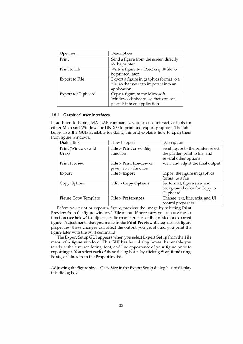
The Export Setup GUI appears when you select Export Setup from the Filemenu of a figure window. This GUI has four dialog boxes that enable youto adjust the size, rendering, font, and line appearance of your figure prior toexporting it. You select each of these dialog boxes by clicking Size, Rendering,Fonts, or Lines from the Properties list.

Adjusting the figure size Click Size in the Export Setup dialog box to displaythis dialog box.

23

The Size dialog box modifies the size of the figure as it will appear whenimported from the export file into your application. If you leave the Width andHeight settings on auto, the figure remains the same size as it appears on yourscreen. You can change the size of the figure by entering new values in theWidth and Height text boxes and then clicking Apply to Figure. To go back tothe original settings, click Restore Figure.

Adjusting the rendering Click Rendering in the Export Setup dialog box todisplay this dialog box.

You can change the settings in this dialog box as follows.

• Colorspace. Use the drop-down list to select a colorspace. Your choices

24

are:

– Black and white

– Grayscale

– RGB color

– CMYK color

• Custom Color. Click the check box and enter a color to be used for thefigure background. Valid entries are:

– white, yellow, magenta, red, cyan, green, blue, or black

– Abbreviated name for the same colors — w, y, m, r, c, g, b, k

– Three-element RGB value — examples: [1 0 1] is magenta. [0 .5 .4] isa dark shade of green.

• Custom Renderer. Click the check box and select a renderer from thedrop-down list:

– painters (vector format)

– OpenGL (bitmap format)

– Z-buffer (bitmap format)

• Resolution. You can select one of the following from the drop-down list:

– Screen — The same resolution as used on your screen display

– A specific numeric setting — 150, 300, or 600 dpi

– auto — automatic selection of a suitable setting

• Keep axis limits. Click the check box to keep axis tick marks and limitsas shown. If unchecked, automatically adjust depending on figure size.

• Show uicontrols. Click the check box to show all user interface controlsin the figure. If unchecked, hide user interface controls.

Changing font characteristics Click Fonts in the Export Setup dialog box todisplay this dialog box.

25

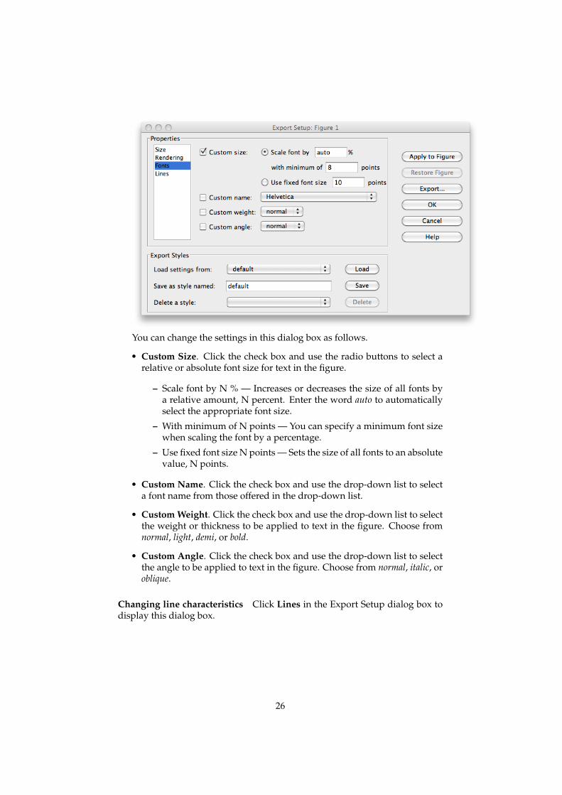
You can change the settings in this dialog box as follows.

• Custom Size. Click the check box and use the radio buttons to select arelative or absolute font size for text in the figure.

– Scale font by N % — Increases or decreases the size of all fonts bya relative amount, N percent. Enter the word auto to automaticallyselect the appropriate font size.

– With minimum of N points — You can specify a minimum font sizewhen scaling the font by a percentage.

– Use fixed font size N points — Sets the size of all fonts to an absolutevalue, N points.

• Custom Name. Click the check box and use the drop-down list to selecta font name from those offered in the drop-down list.

• Custom Weight. Click the check box and use the drop-down list to selectthe weight or thickness to be applied to text in the figure. Choose fromnormal, light, demi, or bold.

• Custom Angle. Click the check box and use the drop-down list to selectthe angle to be applied to text in the figure. Choose from normal, italic, oroblique.

Changing line characteristics Click Lines in the Export Setup dialog box todisplay this dialog box.

26

You can change the settings in this dialog box as follows.

• Custom width. Click the check box and use the radio buttons to select arelative or absolute line size for the figure.

– Scale line width by N % — Increases or decreases the width of alllines by a relative amount, N percent. Enter the word auto to auto-matically select the appropriate line width.

– With minimum of N points — Specify a minimum line width whenscaling the font by a percentage.

– Use fixed line width N points — Sets the width of all lines to anabsolute value, N points.

Convert solid lines to cycle through line styles. When colored graphicsare imported into an application that does not support color, lines that couldformerly be distinguished by unique color are likely to appear the same. Forexample, a red line that shows an input level and a blue line showing outputboth appear as black when imported into an application that does not supportcolored graphics. Clicking this check box causes exported lines to have differ-ent line styles, such as solid, dotted, or dashed lines rather than differentiatingbetween lines based on color.

Saving and Loading Settings If you think you might use these export set-tings at another time, you can save them now and reload them later. At thebottom of each Export Setup dialog box, there is a panel labeled Export Styles.To save your current export styles, type a name into the Save as style namedtext box, and then click Save. If you then click the Load settings from drop-down list, the name of the style you just saved appears among the choices ofexport styles you can load. To load a style, select one of the choices from thislist and then click Load. To delete any style you no longer have use for, selectthat style name from the Delete a style drop-down list and click Delete.

27

Exporting the figure When you finish setting the export style for your figure,you can export the figure to a file by clicking the Export button on the right sideof any of the four Export Setup dialog boxes. As new window labeled Save Asopens. Select a folder to save the file in from the Save in list at the top. Select afile type for your file from the Save as type drop-down list at the bottom, andthen enter a file name in the File name text box. Click the Save button to exportthe file.

1.8.2 Command line interface

You can print a MATLAB figure from the command line or from a MATLABfile. Use the set function to set the properties that control how the printed figurelooks. Use the print function to specify the output format and start the print orexport operation.

The set function changes the values of properties that control the look of afigure and objects within it. These properties are stored with the figure; someare also properties of children such as axes or annotations. When you changeone of the properties, the new value is saved with the figure and affects thelook of the figure each time you print it until you change the setting again.

To change the print properties of the current figure, the set command hasthe form

set(gcf, ’Property1’, value1, ’Property2’, value2, ...)

where gcf is a function call that returns the handle of the current figure, andeach property value pair consists of a named property followed by the valueto which the property is set. For example,

set(gcf, ’PaperUnits’, ’centimeters’, ’PaperType’, ’A4’, ...)

sets the units of measure and the paper size.The print function performs any of the four actions shown in the table be-

low. You control what action is taken, depending on the presence or absence ofcertain arguments.

Action Print commandPrint a figure to a printer printPrint a figure to a file for later printing print filenameCopy a figure in graphics format tothe clipboard

print -dfileformat

Export a figure to a graphics formatfile that you can later import into anapplication

print -dfileformat filename

You can also include optional arguments with the print command. For ex-ample, to export Figure No. 2 to file spline2d.eps, with 600 dpi resolution, andusing the EPS color graphics format, use

print -f2 -r600 -depsc spline2d

The functional form of this command is

print(’-f2’, ’-r600’, ’-depsc’, ’spline2d’);

28

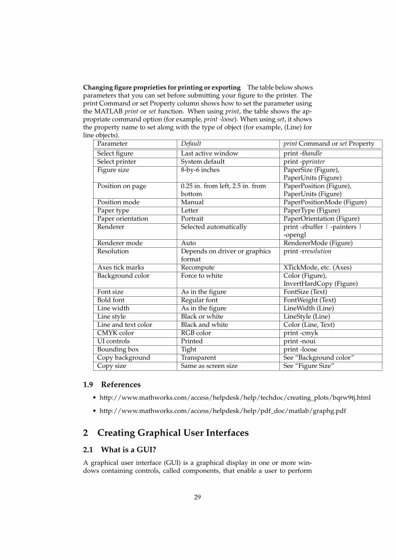
Changing figure proprieties for printing or exporting The table below showsparameters that you can set before submitting your figure to the printer. Theprint Command or set Property column shows how to set the parameter usingthe MATLAB print or set function. When using print, the table shows the ap-propriate command option (for example, print -loose). When using set, it showsthe property name to set along with the type of object (for example, (Line) forline objects).

Parameter Default print Command or set PropertySelect figure Last active window print -fhandleSelect printer System default print -pprinterFigure size 8-by-6 inches PaperSize (Figure),

PaperUnits (Figure)Position on page 0.25 in. from left, 2.5 in. from

bottomPaperPosition (Figure),PaperUnits (Figure)

Position mode Manual PaperPositionMode (Figure)Paper type Letter PaperType (Figure)Paper orientation Portrait PaperOrientation (Figure)Renderer Selected automatically print -zbuffer | -painters |

-openglRenderer mode Auto RendererMode (Figure)Resolution Depends on driver or graphics

formatprint -rresolution

Axes tick marks Recompute XTickMode, etc. (Axes)Background color Force to white Color (Figure),

InvertHardCopy (Figure)Font size As in the figure FontSize (Text)Bold font Regular font FontWeight (Text)Line width As in the figure LineWidth (Line)Line style Black or white LineStyle (Line)Line and text color Black and white Color (Line, Text)CMYK color RGB color print -cmykUI controls Printed print -nouiBounding box Tight print -looseCopy background Transparent See “Background color”Copy size Same as screen size See “Figure Size”

1.9 References

• http://www.mathworks.com/access/helpdesk/help/techdoc/creating_plots/bqrw9tj.html

• http://www.mathworks.com/access/helpdesk/help/pdf_doc/matlab/graphg.pdf

2 Creating Graphical User Interfaces

2.1 What is a GUI?

A graphical user interface (GUI) is a graphical display in one or more win-dows containing controls, called components, that enable a user to perform

29

interactive tasks. The user of the GUI does not have to create a script or typecommands at the command line to accomplish the tasks. Unlike coding pro-grams to accomplish tasks, the user of a GUI need not understand the detailsof how the tasks are performed. GUI components can include menus, toolbars,push buttons, radio buttons, list boxes, and sliders—just to name a few. GUIscreated using MATLAB tools can also perform any type of computation, readand write data files, communicate with other GUIs, and display data as tablesor as plots.

Most GUIs wait for their user to manipulate a control, and then respondto each action in turn. Each control, and the GUI itself, has one or more user-written routines (executable MATLAB code) known as callbacks, named for thefact that they “call back” to MATLAB to ask it to do things. The execution ofeach callback is triggered by a particular user action such as pressing a screenbutton, clicking a mouse button, selecting a menu item, typing a string or a nu-meric value, or passing the cursor over a component. The GUI then respondsto these events. You, as the creator of the GUI, provide callbacks which definewhat the components do to handle events. This kind of programming is oftenreferred to as event-driven programming. In the example, a button click is onesuch event. In event-driven programming, callback execution is asynchronous,that is, it is triggered by events external to the software. In the case of MATLABGUIs, most events are user interactions with the GUI, but the GUI can respondto other kinds of events as well, for example, the creation of a file or connectinga device to the computer.

2.2 Ways to build MATLAB GUIs

A MATLAB GUI is a figure window to which you add user-operated controls.You can select, size, and position these components as you like. Using call-backs you can make the components do what you want when the user clicksor manipulates them with keystrokes. You can build MATLAB GUIs in twoways:

• Use GUIDE (GUI Development Environment), an interactive GUI con-struction kit.

• Create code files that generate GUIs as functions or scripts (program-matic GUI construction).

The first approach starts with a figure that you populate with components fromwithin a graphic layout editor. GUIDE creates an associated code file contain-ing callbacks for the GUI and its components. GUIDE saves both the figure (asa FIG-file) and the code file. Opening either one also opens the other to run theGUI.

In the second, programmatic, GUI-building approach, you create a code filethat defines all component properties and behaviors; when a user executes thefile, it creates a figure, populates it with components, and handles user inter-actions. The figure is not normally saved between sessions because the code inthe file creates a new one each time it runs. As a result, the code files of the twoapproaches look different.

Programmatic GUI files are generally longer, because they explicitly defineevery property of the figure and its controls, as well as the callbacks. GUIDE

30

GUIs define most of the properties within the figure itself. They store the defi-nitions in its FIG-file rather than in its code file. The code file contains callbacksand other functions that initialize the GUI when it opens.

2.3 Creating a simple GUI with GUIDE

This section shows you how to create the graphical user interface (GUI) shownin the following figure. using GUIDE.

The GUI contains:

• An axes component

• A pop-up menu listing three different data sets that correspond to MAT-LAB functions: peaks, membrane, and sinc

• A static text component to label the pop-up menu

• Three push buttons, each of which displays a different type of plot: sur-face, mesh, and contour

2.3.1 Laying out the GUI with GUIDE

• Start GUIDE by typing:

>> guide

at the MATLAB prompt. The GUIDE Quick Start dialog displays, asshown in the following figure.

31

• In the Quick Start dialog, select the Blank GUI (Default) template. ClickOK to display the blank GUI in the Layout Editor, as shown in the fol-lowing figure.

• Display the names of the GUI components in the component palette. Se-lect Preferences from the MATLAB File menu. Then select GUIDE >Show names in component palette, and click OK. The Layout Editor

32

then appears as shown in the following figure.

• Set the size of the GUI by resizing the grid area in the Layout Editor. Clickthe lower-right corner and drag it until the GUI is approximately 3 incheshigh and 4 inches wide. If necessary, make the window larger.

33

• Add three push buttons, a static text area, a pop-up menu, and an axesto the GUI. Select the corresponding entries from the component paletteat the left side of the Layout Editor and drag them into the layout area.Position all controls approximately as shown in the following figure.

34

• If several components have the same parent, you can use the AlignmentTool to align them to one another. To align the three push buttons:

1. Select all three push buttons by pressing Ctrl and clicking them.

2. Select Align Objects from the Tools menu to display the AlignmentTool.

3. Make these settings in the Alignment Tool, as shown in the follow-ing figure:

– 20 pixels spacing between push buttons in the vertical direction.– Left-aligned in the horizontal direction.

35

• Use the Alignment Tool to align and distribute all controls in the figure.

• The push buttons, pop-up menu, and static text have default labels whenyou create them. Their text is generic, for example Push Button 1. Changethe text to be specific to your GUI, so that it explains what the componentis for.

• To change the text of the first Push Button:

1. Select Property Inspector from the View menu.

2. In the layout area, click the Push Button you want to modify.

3. In the Property Inspector, select the String property and then replacethe existing value with the word Surf.

4. Select each of the remaining push buttons in turn and repeat steps 2and 3. Label the middle push button Mesh, and the bottom buttonContour.

36

• The pop-up menu provides a choice of three data sets: peaks, membrane,and sinc. These data sets correspond to MATLAB functions of the samename. To list those data sets as choices in the pop-menu:

1. In the layout area, select the pop-up menu by clicking it.

2. In the Property Inspector, click the button next to String. The Stringdialog box displays.

3. Replace the existing text with the names of the three data sets: Peaks,Membrane, and Sinc. Press Enter to move to the next line.

4. When you have finished editing the items, click OK. The first itemin your list, Peaks, appears in the pop-up menu in the layout area.

37

• In this GUI, the static text serves as a label for the pop-up menu. The usercannot change this text. This topic shows you how to change the statictext to read Select Data.

1. In the layout area, select the static text by clicking it.

2. In the Property Inspector, click the button next to String. In theString dialog box that displays, replace the existing text with thephrase Select Data.

3. Click OK. The phrase Select Data appears in the static text compo-nent above the pop-up menu.

• In the Layout Editor, your GUI now looks like in the following figure,and the next step is to save the layout.

38

• When you save a GUI, GUIDE creates two files, a FIG-file and a code file.The FIG-file, with extension .fig, is a binary file that contains a descrip-tion of the layout. The code file, with extension .m, contains MATLABfunctions that control the GUI.

• To save a GUI you can either choose Save as... from the File menu or Runit (from the Tools menu). If you try to run an unsaved Figure, GUIDE willask you to save it first. Save the Figure as simpleGUI.fig (in the currentpath): GUIDE saves the files simpleGUI.fig and simpleGUI.m. The latterfile is opened in the Editor.

• Run the figure by choosing Tools > Run or from the MATLAB console, bytyping:

>> simpleGUI

• Now the GUI is designed, but it does not do anything!

2.3.2 Adding code to the GUI

When you saved your GUI in the previous section, GUIDE created two files:a FIG-file simpleGUI.fig that contains the GUI layout and a file, simpleGUI.m,

39

that contains the code that controls how the GUI behaves. The code consistsof a set of MATLAB functions (that is, it is not a script). But the GUI did notrespond because the functions contain no statements that perform actions yet.

Here we will see how to add code to the file to make the GUI do things.

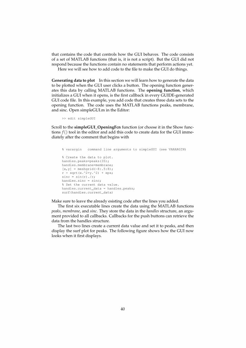
Generating data to plot In this section we will learn how to generate the datato be plotted when the GUI user clicks a button. The opening function gener-ates this data by calling MATLAB functions. The opening function, whichinitializes a GUI when it opens, is the first callback in every GUIDE-generatedGUI code file. In this example, you add code that creates three data sets to theopening function. The code uses the MATLAB functions peaks, membrane,and sinc. Open simpleGUI.m in the Editor:

>> edit simpleGUI

Scroll to the simpleGUI_OpeningFcn function (or choose it in the Show func-tions f () tool in the editor and add this code to create data for the GUI imme-diately after the comment that begins with

% varargin command line arguments to simpleGUI (see VARARGIN)

% Create the data to plot.handles.peaks=peaks(35);handles.membrane=membrane;[x,y] = meshgrid(-8:.5:8);r = sqrt(x.^2+y.^2) + eps;sinc = sin(r)./r;handles.sinc = sinc;% Set the current data value.handles.current_data = handles.peaks;surf(handles.current_data)

Make sure to leave the already esisting code after the lines you added.The first six executable lines create the data using the MATLAB functions

peaks, membrane, and sinc. They store the data in the handles structure, an argu-ment provided to all callbacks. Callbacks for the push buttons can retrieve thedata from the handles structure.

The last two lines create a current data value and set it to peaks, and thendisplay the surf plot for peaks. The following figure shows how the GUI nowlooks when it first displays.

40

Programming the popup menu The pop-up menu enables the user to selectthe data to plot. When the GUI user selects one of the three plots, MATLAB setsthe pop-up menu Value property to the index of the selected string. The pop-up menu callback reads the pop-up menu Value property to determine the itemthat the menu currently displays, and sets handles.current_data accordingly.

• To program the pop-up menu callback, right-click on the pop-up menuin GUIDE and select View Callbacks > Callback.

• This will display the popupmenu1_Callback() function in the Editor.

• Add the following code to the popupmenu1_Callback() after the comments.This code first retrieves two pop-up menu properties:

– String — a cell array that contains the menu contents

– Value — the index into the menu contents of the selected data set

It then uses a switch statement to make the selected data set the currentdata. The last statement saves the changes to the handles structure.

% Determine the selected data set.str = get(hObject, ’String’);val = get(hObject,’Value’);% Set current data to the selected data set.switch str{val}case ’Peaks’ % User selects peaks.handles.current_data = handles.peaks;

case ’Membrane’ % User selects membrane.handles.current_data = handles.membrane;

case ’Sinc’ % User selects sinc.handles.current_data = handles.sinc;

41

end% Save the handles structure.guidata(hObject,handles)

Programming the push buttons Each of the push buttons creates a differenttype of plot using the data specified by the current selection in the pop-upmenu. The push button callbacks get data from the handles structure and thenplot it.

• Right-click the Surf push button in the Layout Editor to display a contextmenu. From that menu, select View Callbacks > Callback.

• This will display the pushbutton1_Callback() function in the Editor.

• Add the following code to the pushbutton1_Callback() after the comments:

% Display surf plot of the currently selected data.surf(handles.current_data);

• Repeat previous steps for the Mesh push button and add this code to thepushbutton2_Callback():

% Display mesh plot of the currently selected data.mesh(handles.current_data);

• Repeat previous steps for the Contour push button and add this code tothe pushbutton3_Callback():

% Display contour plot of the currently selected data.contour(handles.current_data);

• Save the simpleGUI.m file.

Running the GUI Run the GUI from the MATLAB console.

>> simpleGUI;

2.4 Creating a simple GUI programmatically

In this section we will create the same GUI as in the previous one, but withoutusing GUIDE.

2.4.1 Creating a GUI code file

We will start by creating the backbone of our M-file. In the MATLAB consoletype:

>> edit simpleGUI2

and add the following code in the file:

function simpleGUI2% SIMPLEGUI2 Select a data set from the pop-up menu, then% click one of the plot-type push buttons. Clicking the button% plots the selected data in the axes.end

Save the file in the current path.

42

2.4.2 Laying out a simple GUI

Creating the figure In MATLAB, a GUI is a figure. This first step creates thefigure and positions it on the screen. It also makes the GUI invisible so that theGUI user cannot see the components being added or initialized. When the GUIhas all its components and is initialized, the example makes it visible.

% Initialize and hide the GUI as it is being constructed.f = figure(’Visible’,’off’,’MenuBar’,’None’,’Position’,[360,500,450,285]);

The call to the figure function uses two property/value pairs. The Position prop-erty is a four-element vector that specifies the location of the GUI on the screenand its size: [distance from left, distance from bottom, width, height]. Add the pre-vious code right after the initial comments in simpleGUI2.m.

Adding the components The example GUI has six components: three pushbuttons, one static text, one pop-up menu, and one axes. Start by writing state-ments that add these components to the GUI. Create the push buttons, statictext, and pop-up menu with the uicontrol function. Use the axes function tocreate the axes.

• Add the three push buttons to your GUI by adding these statements toyour code file following the call to figure.

% Construct the components.hsurf = uicontrol(’Style’,’pushbutton’,...

’String’,’Surf’,’Position’,[315,220,70,25]);hmesh = uicontrol(’Style’,’pushbutton’,...

’String’,’Mesh’,’Position’,[315,180,70,25]);hcontour = uicontrol(’Style’,’pushbutton’,...

’String’,’Countour’,’Position’,[315,135,70,25]);

These statements use the uicontrol function to create the push buttons.Each statement uses a series of property/value pairs to define a push but-ton:

– Style — In the example, pushbutton specifies the component as apush button.

– String — Specifies the label that appears on each push button. Here,there are three types of plots: Surf, Mesh, Contour.

– Position — Uses a four-element vector to specify the location of eachpush button within the GUI and its size: [distance from left, distancefrom bottom, width, height]. Default units for push buttons are pixels.

Each call returns the handle of the component that is created (hsurf, hmesh,hcontour).

• Add the pop-up menu and its label to your GUI by adding these state-ments to the code file following the push button definitions.

hpopup = uicontrol(’Style’,’popupmenu’,...’String’,{’Peaks’,’Membrane’,’Sinc’},...’Position’,[300,50,100,25]);

htext = uicontrol(’Style’,’text’,’String’,’Select Data’,...’Position’,[325,90,60,15]);

43

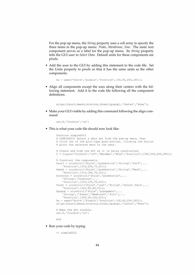
For the pop-up menu, the String property uses a cell array to specify thethree items in the pop-up menu: Peaks, Membrane, Sinc. The static textcomponent serves as a label for the pop-up menu. Its String propertytells the GUI user to Select Data. Default units for these components arepixels.

• Add the axes to the GUI by adding this statement to the code file. Setthe Units property to pixels so that it has the same units as the othercomponents.

ha = axes(’Units’,’pixels’,’Position’,[50,60,200,185]);

• Align all components except the axes along their centers with the fol-lowing statement. Add it to the code file following all the componentdefinitions.

align([hsurf,hmesh,hcontour,htext,hpopup],’Center’,’None’);

• Make your GUI visible by adding this command following the align com-mand.

set(f,’Visible’,’on’)

• This is what your code file should now look like:

function simpleGUI2% SIMPLEGUI2 Select a data set from the pop-up menu, then% click one of the plot-type push buttons. Clicking the button% plots the selected data in the axes.

% Create and hide the GUI as it is being constructed.f = figure(’Visible’,’off’,’MenuBar’,’None’,’Position’,[360,500,450,285]);

% Construct the components.hsurf = uicontrol(’Style’,’pushbutton’,’String’,’Surf’,...

’Position’,[315,220,70,25]);hmesh = uicontrol(’Style’,’pushbutton’,’String’,’Mesh’,...

’Position’,[315,180,70,25]);hcontour = uicontrol(’Style’,’pushbutton’,...

’String’,’Countour’,...’Position’,[315,135,70,25]);

htext = uicontrol(’Style’,’text’,’String’,’Select Data’,...’Position’,[325,90,60,15]);

hpopup = uicontrol(’Style’,’popupmenu’,...’String’,{’Peaks’,’Membrane’,’Sinc’},...’Position’,[300,50,100,25]);

ha = axes(’Units’,’Pixels’,’Position’,[50,60,200,185]);align([hsurf,hmesh,hcontour,htext,hpopup],’Center’,’None’);

% Make the GUI visible.set(f,’Visible’,’on’)

end

• Run your code by typing

>> simpleGUI2

44

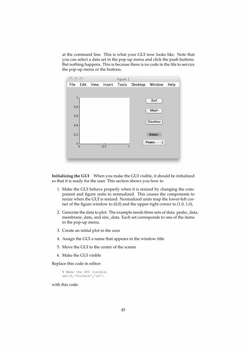
at the command line. This is what your GUI now looks like. Note thatyou can select a data set in the pop-up menu and click the push buttons.But nothing happens. This is because there is no code in the file to servicethe pop-up menu or the buttons.

Initializing the GUI When you make the GUI visible, it should be initializedso that it is ready for the user. This section shows you how to

1. Make the GUI behave properly when it is resized by changing the com-ponent and figure units to normalized. This causes the components toresize when the GUI is resized. Normalized units map the lower-left cor-ner of the figure window to (0,0) and the upper-right corner to (1.0, 1.0).

2. Generate the data to plot. The example needs three sets of data: peaks_data,membrane_data, and sinc_data. Each set corresponds to one of the itemsin the pop-up menu.

3. Create an initial plot in the axes

4. Assign the GUI a name that appears in the window title

5. Move the GUI to the center of the screen

6. Make the GUI visible

Replace this code in editor:

% Make the GUI visible.set(f,’Visible’,’on’)

with this code:

45

% Initialize the GUI.

% Change units to normalized so components resize automatically.set([f,ha,hsurf,hmesh,hcontour,htext,hpopup],’Units’,’normalized’);

% Generate the data to plot.peaks_data = peaks(35);membrane_data = membrane;[x,y] = meshgrid(-8:.5:8);r = sqrt(x.^2+y.^2) + eps;sinc_data = sin(r)./r;

% Create a plot in the axes.current_data = peaks_data;surf(current_data);

% Assign the GUI a name to appear in the window title.set(f,’Name’,’Simple GUI’)

% Move the GUI to the center of the screen.movegui(f,’center’)

% Make the GUI visible.set(f,’Visible’,’on’);

• Run your code by typing simpleGUI2 at the command line. The initial-ization above cause it to display the default peaks data with the surf func-tion, making the GUI look like this.

Programming the pop-up menu The pop-up menu enables users to select thedata to plot. When a GUI user selects one of the three data sets, MATLAB setsthe pop-up menu Value property to the index of the selected string. The pop-upmenu callback reads the pop-up menu Value property to determine which itemis currently displayed and sets current_data accordingly. Add the followingcallback to your file following the initialization code and before the final endstatement.

46

% Pop-up menu callback. Read the pop-up menu Value property to% determine which item is currently displayed and make it the% current data. This callback automatically has access to% current_data because this function is nested at a lower level.function popup_menu_Callback(source,eventdata)% Determine the selected data set.str = get(source, ’String’);val = get(source,’Value’);% Set current data to the selected data set.switch str{val}case ’Peaks’ % User selects Peaks.current_data = peaks_data;

case ’Membrane’ % User selects Membrane.current_data = membrane_data;

case ’Sinc’ % User selects Sinc.current_data = sinc_data;

endend

Programming the push buttons Each of the three push buttons creates a dif-ferent type of plot using the data specified by the current selection in the pop-up menu. The push button callbacks plot the data in current_data. They auto-matically have access to current_data because they are nested at a lower level.Add the following callbacks to your file following the pop-up menu callbackand before the final end statement.

% Push button callbacks. Each callback plots current_data in the% specified plot type.function surfbutton_Callback(source,eventdata)% Display surf plot of the currently selected data.surf(current_data);

endfunction meshbutton_Callback(source,eventdata)% Display mesh plot of the currently selected data.mesh(current_data);

endfunction contourbutton_Callback(source,eventdata)% Display contour plot of the currently selected data.contour(current_data);

end

Associating callbacks to their components When the GUI user selects a dataset from the pop-up menu or clicks one of the push buttons, MATLAB softwareexecutes the callback associated with that particular event. But how does thesoftware know which callback to execute? You must use each component’sCallback property to specify the name of the callback with which it is associated.

• To the uicontrol statement that defines the Surf push button, add the prop-erty/value pair

’Callback’,{@surfbutton_Callback}

so that the statement looks like this:

hsurf = uicontrol(’Style’,’pushbutton’,’String’,’Surf’,...

47

’Position’,[315,220,70,25],...’Callback’,{@surfbutton_Callback});

Callback is the name of the property. surfbutton_Callback is the name ofthe callback that services the Surf push button.

• Similarly, to the uicontrol statement that defines the Mesh push button,add the property/value pair

’Callback’,{@meshbutton_Callback}

• To the uicontrol statement that defines the Contour push button, add theproperty/value pair

’Callback’,{@contourbutton_Callback}

• To the uicontrol statement that defines the pop-up menu, add the prop-erty/value pair

’Callback’,{@popup_menu_Callback}

Running the GUI Run the GUI by typing the name of the code file at thecommand line.

>> simpleGUI2

2.5 References

• http://www.mathworks.com/access/helpdesk/help/techdoc/creating_guis/bqz79mu.html

• http://www.mathworks.com/access/helpdesk/help/pdf_doc/matlab/buildgui.pdf

48