1

Sesame: Self-Constructive Energy Modeling for Battery-Powered Mobile Systems

Technical Report 2010-1213

Mian Dong and Lin Zhong Dept. of Electrical & Computer Engineering, Rice University

ABSTRACT

System energy models are important for energy opti-mization and management in mobile systems. However, existing system energy models are built in lab with the help from a second computer. Not only are they labor-intensive; but also they will not adequately account for the great di-versity in the hardware and usage of mobile systems. Moreover, existing system energy models are intended for energy estimation for time intervals of one second or long-er; they do not provide the required rate for fine-grain use such as per-application energy accounting.

In this work, we study a self-modeling paradigm in which a mobile system automatically generates its energy model without any external assistance. Our solution, Se-same, leverages the possibility of self power measurement through the smart battery interface and employs a suite of novel techniques to achieve accuracy and rate much higher than that of the smart battery interface.

We report the implementation and evaluation of Se-same on a laptop and a smartphone. The experiment results show that Sesame generates system energy models of 95% accuracy at one estimation per second and 88% accuracy at one estimation per 10ms, without any external assistance. A five-day field study with four laptop users further de-monstrates the effectiveness, efficiency, and noninvasive-ness of Sesame.

1. Introduction An energy model estimates the energy consumption by

a mobile system in a given time period. Mathematically, an energy model can be represented by a function such that

  , , … , ,

where is the energy consumption in time interval and , , …, are the system behavior data for the same period that can be read in software. To use the terminology of regression analysis, is the response of the model and , ,…, are the predictors. Most system energy models employ a linear function for

. The most important metrics of a model is accuracy and rate, or the reciprocal of the time interval t for which the energy consumption is modeled. While the importance of a high accuracy is obvious, a high rate is also important for many reasons. First, per-application energy accounting a multitasking system, which requires energy estimation for time intervals of 10ms or shorter or at 100Hz. Per-

application energy accounting is useful not only for detect-ing rogue applications [1] but also for incentive mechan-isms for applications that require a mobile device to con-sume energy for a goal beyond serving its owner, e.g., par-ticipatory sensing [2, 3] and cooperative communication [4]. Second, energy models are the foundation to energy management and optimization in operating systems (OS) [5-8] and software [9].

Existing system energy modeling approaches are how-ever fundamentally limited in two important ways. First, all existing methods generate the model of a system in the lab using high quality external power measurements. Such methods are not only labor-intensive but also produce fixed energy models that are determined by the workload used in model construction. Modern mobile systems such as smartphones and laptops challenge such methods as will be analyzed in Section 3. Moreover, while cycle-accurate hardware power models exist, all reported system energy models have a low rate. That is, they estimate energy con-sumption for a time interval of one second or longer. In another word, they estimate energy at a rate of 1Hz or low-er. While they work well for certain objectives, e.g., ther-mal analysis/management and battery lifetime estimation, energy models of 1Hz are fundamentally inadequate for applications such as per-application energy accounting.

Our approach to address these two limitations of exist-ing methods is to enable a mobile system to construct a high-rate system energy model without external assistance. We call this approach self modeling, or Sesame. Instead of using special circuitry for system power measurement, e.g., [10, 11], our key idea to leverage the smart battery inter-face already available on mobile systems.

Toward realizing Sesame, we answer two technical questions in this work. First, can battery interfaces provide the necessary accuracy and rate for the energy models from 1Hz to 100Hz? We report an extensive characteriza-tion study of the battery interfaces of existing mobile sys-tems, reveal their fundamental limitations in accuracy and rate, and suggest methods to overcome them. In particular, we leverage the linearity of the energy model and random nature of battery interface error to devise a model molding method that achieves high accuracy and high rate when combined with principal component analysis. Second, how can we realize Sesame on resource-limited mobile devices? With improved data collection support and properly sche-duled model construction, we show that Sesame can be

2

realized with negligible overhead and without intruding normal usage.

We implement Sesame for both laptop computers and smartphones. We evaluate the implementation both in lab and through two five-day field studies with four laptop users and four smartphone users, respectively, and com-pare the generated models against accurate external mea-surement. The evaluation shows that Sesame can automati-cally generate and adapt energy models. For a Thinkpad T61 laptop, Sesame achieves an accuracy of 88% at 100Hz and 95% at 1Hz, with a battery interface of only 0.5Hz and without any external assistance; Sesame also achieves an accuracy of 82% at 100Hz and 88% at 1Hz for a Nokia N900 smartphone with a battery interface only of 0.1Hz. The accuracy of the models generated by Sesame is com-parable with that by state-of-the-art system energy model-ing work employing a second system for measurement. Moreover, our two field studies of four laptop users and four smartphone users show that Sesame is able to build such energy models without interrupting users.

In summary, we make the following research contribu-tions in building Sesame.

A characterization of battery interfaces on modern mobile devices and their limitations.

A suite of techniques to overcome the limitations of battery interfaces and fuel gauge ICs for self energy modeling for a rate up to 100Hz.

The realization and evaluation of Sesame that auto-matically constructs accurate and fine-grain energy models using the battery interface.

The rest of the paper is organized as follows. Section 2 discusses related work in system energy modeling. Section 3 provides motivations to the proposed self-modeling ap-proach. Section 4 reports our characterization of smart bat-tery interfaces on commercial mobile systems. Section 5 offers the design of Sesame and its key technical compo-nents in order to address the limitations of the smart battery interfaces and reduce the overhead of self model construc-tion. Section 6 describes the implementation details of Se-same. Section 7 evaluates the Sesame through both lab and field-based studies. Sections 8 and 9 discuss the limitations of Sesame and conclude the paper, respectively.

2. Related Work and Background There is an extensive body of literature on system

energy modeling. All existing methods except [12] are based on external assistance. That is, they all employ a second computer to collect power measurement of the tar-get system. We note that many computing systems can directly measure their own power consumption. For exam-ple, power supply units of high-end systems are often equipped with a power meter that can be digitally con-nected to the system. Modern battery-powered systems can acquire system power consumption from the smart battery

interface. The authors of [10] leverage the special property of switching regulators to measure the energy output of a switching regulator. Such self power measurement is the prerequisite to self energy modeling.

There are two major approaches toward system energy modeling. The first is component-wise [5, 6, 8, 13-15]. That is, they calculate the system energy based on aggre-gating the energy consumption by major system compo-nents. This approach suffers in that there are components that are invisible to the model or the OS. Measurement of modern mobile systems [16] has shown that “invisible” components such as the northbridge and southbridge can account for as much as 50% of the system energy con-sumption. Therefore, Sesame takes the second group’s approach, which to model the system energy consumption without the models of each component, or integral model-ing [17, 18]. This approach treats the system as a whole without breaking it down to components.

Moreover, existing system energy modeling methods give energy estimation at a fixed, low rate, such as one per minute [19], one per several seconds [6], and one per second (1Hz) [17, 18, 20]. In contrast, Sesame is able to generate energy models with much higher rates; it achieves 88% accuracy at 100Hz with a battery interface of only 0.5Hz. It is worth noting that energy models for a system component, e.g., processor [21, 22] and memory [23], can achieve much higher rates, often cycle-accurate. Yet such models require circuit-level power characterization, which is impractical to system energy modeling.

A very recent work reports Joulemeter, a system that builds power models of virtual machines using built-in power sensors coming with servers [12]. Joulemeter does share our philosophy of self-modeling. But Joulemeter is inadequate for the goal of Sesame for three important rea-sons. (i) Most importantly, Joulemeter gives one estimation per two seconds (0.5Hz), inadequate for applications such as per-process energy accounting. A key novelty of Se-same lies in its combination of model molding and PCA to realize one estimation per 10ms (100Hz). (ii) Joulemeter employs a linear model with fixed predictors known befo-rehand to dominate a server’s power consumption. In con-trast, Sesame is truly adaptive by statistically/automatically selecting the best predictors. Sesame’s adaptation is impor-tant to mobile devices where hardware/usage diversity is high. (iii) Joulemeter employs an expensive calibration to construct the model, making it inherently inefficient for adaptation achieved by Sesame.

3. Why Self Modeling? We next highlight the dependencies of energy models

on the configuration, usage and even the battery of a mo-bile system and therefore motivate the proposed self-modeling approach. Out of simplicity, we use the 1Hz energy model from [20, 24] based on CPU utilization. Our target system is a Thinkpad T61 laptop. We measure its

3

power with a USB-2533 Data Acquisition System from Measurement Computing along with another PC.

3.1 Dependency on Hardware Energy models may change due to hardware change.

For example, if more memory is added, the system power consumption will likely increase, given the same CPU uti-lization. We study three hardware configurations of the T61 laptop with only minor differences, i.e., fixed CPU frequency of 2GHz, fixed CPU frequency of 800MHz; and DVS (dynamic voltage scaling) enabled. Similar to exist-ing modeling methods, we build a calibrator program that switches between busy loops and idle with a controllable duty cycle to produce workload with different CPU utiliza-tions. At each level of CPU utilization, we measure the laptop’s power consumption. Figure 1 (left) presents the linear energy model for each of the hardware configura-tions. It clearly shows that there are considerable differ-ences (up to 25%) among three models. This simple exam-ple demonstrates the generic dependency of energy models on hardware configuration. We note that the model differ-ence in this particular example can be eliminated by adding CPU frequency as a predictor. However, it is impractical to include all predictors that can account for every hardware detail because not all hardware components are visible to the OS and collecting the values of a large number of pre-dictors would incur significant overhead.

3.2 Dependency on Usage Using the same setup, we next illustrate how usage of

the system can impact its energy model. Different software may invoke different hardware components. Since some components are invisible to the OS, difference in invisible components induced by software will not be noticed by the OS. To demonstrate the usage dependency, we build three linear models by running three different benchmarks: the dummy calibrator described above, a SW Developer benchmark (Developer), and a Media Player benchmark (Player), both of the latter two from the Linux Battery Life Toolkit (BLTK) [25]. As shown in Figure 1 (right), the difference among their estimations can be as high as 25%. Again, one may argue that such difference can be reduced by incorporating as many benchmarks as possible into a factory-built model. However, using more benchmarks will lead to a model that generalizes decently but does not achieve high accuracy for the most common usage. As the usage of mobile systems by different users can be very different [26] and the usage by the same user can evolve over time [27], factory-built models are unlikely to provide an improved accuracy for all users and all usage.

3.3 Dependency on Battery The energy consumption of a battery-powered system

is impacted by the internal resistance of the battery, which varies from battery to battery. To illustrate this, we use two G1 smartphones (Phone 1 and Phone 2) and two batteries

(Battery 1 and Battery 2) for four combinations. We build an energy model similar to that used in [18] for Phone 1 and battery 1 and test the model on all four combinations. In all the tests, we use the same benchmark described in Section 4. Table 1 provides the root mean square (RMS) of relative errors for each combination. As shown in the table, the error of the linear model is as low as 5% on Phone 1+Battery 1 where the model is built. And the model works pretty accurate, error less than 7%, on Phone 2+Battery 1. However, the error almost doubles when Battery 2 is used.

The dependencies of the system energy models on configuration, usage, and battery suggest “personalized” models be built for a mobile system, which is only possible through a self-modeling approach.

4. Battery Interface Characterization We next provide an experimental characterization of

smart battery interfaces available in modern mobile sys-tems. We focus on their limitations in accuracy and rate in order to suggest solutions.

4.1 Smart Battery Interface Primer Most batteries of modern mobile systems employ the

smart battery interface in order to support intelligent charg-ing, battery safety, and battery lifetime estimation [28].

A smart battery interface includes both hardware and software components. The key hardware of a smart battery interface is a fuel gauge IC that measures battery voltage, temperature, and maybe current. The fuel gauge IC esti-mates the remaining battery capacity with one of the fol-lowing two methods. The first employs a built-in battery model that estimates remaining capacity using the voltage and temperature, e.g., Maxim MAX17040. The other me-thod measures the discharge current using a sense resistor, e.g., Maxim DS2760 and TI BQ20z70. By periodically measuring the discharge current, the fuel gauge IC can

Figure 1: Linear system energy models based on CPU utilization with (left) different configurations and (right) different usage

Table 1: RMS error of an energy model lab-built with Phone 1+Battery 1 for four phone-battery combinations.

Phone 1 Phone 2 Battery 1 5% 7% Battery 2 11% 12%

15

20

25

30

35

40

0% 50% 100%

System power (W

)

CPU utilization

DVFS Enabled800 MHz2GHz

15

20

25

30

35

40

0% 50% 100%

System power (W

)

CPU utilization

CalibraterDeveloperPlayer

4

count the total charges drawn from the battery and calcu-late the remaining capacity accordingly. Apparently, a smart battery interface with current measurement capabili-ty is much better for self energy measurement.

In software, the fuel gauge IC exposes several regis-ters that store the values of temperature, voltage, remaining capacity, and sometimes discharge current, of the battery and updates these registers periodically. The OS, often through ACPI, provides a battery driver that can read such registers through a serial bus such as SMBus and I2C. Li-nux employs a virtual file system for the readings from the battery driver so that applications can access battery infor-mation through a standard file system read API.

4.2 Experimental Setup To investigate the accuracy and rate of battery inter-

face readings, we have characterized three types of mobile systems, i.e., laptop, smartphone and PDA, as summarized by Table 2. In the characterization, we employ a set of benchmark applications for each of the mobile system. For laptops and the smartphone with Maemo, we use the BLTK [12]. For other smartphones, we use JBenchmark [13] and 3DMarkMobile [14]. Having each benchmark running, we measure the discharge current out of the bat-tery using 1KHz sampling rate, average every ten samples and use the data, at a rate of 100Hz, as the ground truth (DAQ) to compare with the readings from battery interfac-es. The measurement is performed at the output of the bat-tery with the system being powered by the battery.

4.3 Key Findings We make the following observations. First, there is a

huge variety in the smart battery interfaces on mobile sys-tems. We identify three types. (i) The voltage-based inter-face gives the remaining battery capacity based on the bat-tery output voltage, e.g., Nokia N810 and N900. (ii) The instant interface gives the instant discharge current, such as Nokia N85 (See Figure 2 (a)). (iii) Finally, the filtered in-terface gives a low-pass filtered reading of the discharge current, such as Thinkpad T61. The fuel gauge IC used in T61 battery interface employs a low-pass filter that reports discharge current values by averaging ten readings in last 16 seconds. This low-pass filter effect is illustrated in Fig-ure 2 (b) and is designed to facilitate the estimation of bat-tery lifetime using history [15]. Unlike N85, the battery interface readings of T61 have a delay, around 16 seconds,

than the real values. We note that modern mobile devices are increasingly using the instant interfaces. We further find that different mobile devices have different reading rates in their battery interfaces. That is, they try to give the average discharge current for time intervals of different lengths. The shorter the interval, the higher reading rate the interface has. Table 2 summarizes the battery interface reading rates of all the mobile systems we have characte-rized.

Consequently, our second observation is: the rate of the smart battery interface is low with 4Hz being the high-est observed. The reason is simple: high-rate measurement requires a more expensive and more power-hungry fuel gauge IC, which does not bode well for a cost-sensitive and power-sensitive battery for mobile systems. Some fuel gauge ICs, e.g., TI BQ2019 [29], employ a charge counter, which increases by one unit whenever a certain amount of charge is drawn from the battery. As a result, the higher the current, the faster counter updates, up to 30Hz during peak power consumption. However, because a mobile system consumes moderate or low power in most of the time, the average measurement rate is only 1.138Hz according to the datasheet [29]. The low rate of smart battery interfaces is an important barrier toward our goal of realizing Sesame with high rate (up to 100Hz).

Our third observation is: the error of the instant bat-tery interface reading is high. We use three representative systems, N85, T61 and N900 to demonstrate this. The bat-tery interfaces of N85 and T61 can measure current at 4Hz

Table 2: Battery interface of popular mobile systems

System OS Current

Measurement Reading

Rate Lenovo Thinkpad T61 Linux Yes 0.5 Hz

Dell Latitude D630 Linux Yes 1 Hz Nokia N85/N96 Symbian Yes 4 Hz

Nokia N810/N900 Maemo No (voltage) ~0.1Hz Google G1/Nexus One Android Yes ~0.25Hz

(a)

(b) Figure 2: Current readings from accurate external mea-surement and battery interface for (a) N85; (b) T61

Figure 3: Error vs. rate for battery interface readings

0.1

0.2

0.3

0 30 60 90

Current (A)

Time (s)

Bat I/FDAQ

1

3

5

0 30 60 90

Current (A)

Time (s)

Bat I/FDAQ

0%10%20%30%40%50%

0.01 0.1 1 10 100

RMS of Relative

 Error

Rate (Hz)

N85T61N900

5

and 0.5Hz, respectively. That of N900 does not support direct current measurement but the average current for a period can be calculated from the readings of the remain-ing battery capacity at the beginning and end of the period at 0.1Hz. To evaluate the accuracy of these battery inter-faces, we prepare the ground truth using the measurement from the 100Hz DAQ. For example, to compare with the 4Hz readings from N85, we use the average of the corres-ponding 25 samples collected from the 100Hz DAQ data as the ground truth. Figure 3shows the root mean square (RMS) of all the relative errors for N85 at 4Hz (33%), for T61 at 0.5Hz (19%), and for N900 at 0.1Hz (45%). Such high instant errors pose a great challenge to energy model-ing using smart battery interface readings.

On the other hand, we also observe that the instant er-rors can be reduced by averaging readings to reduce the rate. For example, we can average every four readings from the N85 4Hz battery interface to produce the average current for each second or a 1Hz reading. This 1Hz current reading will have only 10% RMS error compared to 33% at 4Hz. Figure 3 shows the RMS errors for N85, T61, and N900 as the reading rate is reduced down to 0.01Hz or one reading per 100s. The RMS error decreases as the reading rate decreases. There are two reasons for this error reduc-tion. First, random noises in the smart battery interfaces contribute significantly to the instant error. By averaging the instant readings to produce a low reading, the random noise can be canceled out. Second, the low-pass filter em-ployed by a battery interface introduces significant error, e.g., Figure 2 (b) for T61. By averaging the instant read-ings to reduce the reading rate, the reduced rate will ap-proach or even drop below that of the low-pass filter’s cu-toff frequency, which leads to reduced error. We note that the first type of errors will be handled in model building such as linear regression thanks to their randomness; while the second type of errors are dependent on each other and should be treated as random errors. We call the second type of errors systematic errors and treat them specially, as will be described in Section 5.3.

Finally, accessing the battery interface in software contributes little to the system energy consumption in the battery interface reading. To obtain the extra energy con-sumed in battery interface reading, we run each of the benchmark twice. In the first time; we perform the experi-ment as described above, while in the second time, we only measure the power using the USB-2533 Data Acquisition System. Then we compare the average power consumption of the two and the results show that the contribution of battery interface reading is negligible, less than 1% for both systems.

5. Design of Sesame We next provide the design of Sesame and our key

techniques to overcome the limitations of battery interfaces

5.1 Design Goals and Architecture We have the following design goals for Sesame to ca-

ter a broad range of needs in energy models.

Sesame requires no external assistance. It will collect the data traces, identify important predictors, and subse-quently build a model out of them without another com-puter or measurement instrument.

Sesame shall incur low overhead and complexity be-cause it runs when the system is being used. To achieve this, Sesame schedules the computation intensive tasks to run in system idle period when it is on AC power supply. Therefore, only data collection and some simple calcula-tion are performed during system usage.

Sesame should achieve higher accuracy and rate than the battery interface. To serve a broad range of applica-tions of energy models, Sesame should achieve high accu-racy at rates as high as 100Hz. It utilizes several techniques to overcome the limitation set by the battery interface.

Sesame must adapt to changes either in hardware or usage. Sesame monitors the accuracy of the energy model in use and adapts it accordingly when the accuracy is be-low a certain threshold.

Figure 4 presents the architecture of Sesame with three major components: data collector, model constructor, and model manager, described in detail below.

5.2 Data Collector The Sesame data collector interacts with the native OS

to acquire predictors for energy modeling. Only the lowest layer of the data collector is platform-specific. The data collector considers the following system behavior data as widely used in existing system energy modeling work.

First, Sesame uses system statistics, such as CPU tim-ing statistics and memory usage, supported by modern OSes. For example, Linux uses the sys and proc file system to provide information about processor, memory, disk, and process, and the dev file system to provide information of peripherals such as network interface card. Sesame further utilizes the Advanced Configuration and Power Interface (ACPI) available on modern mobile systems. ACPI pro-

Figure 4: Architecture of Sesame with three major components

Data Collector

Sesame

Model Constructor

Predictor transformation

Model

Model manager

Operating System

Bat I/FSTATS

Energy  readings Stats readings 

Predictors Responses

Model molding

Application specific predictors

6

vides platform-independent interfaces for the power state of hardware, including the processor and peripherals. In Linux, the ACPI information can be found in /proc/acpi/. Thanks to ACPI, Sesame is able to access the power status of many system components just as reading a file.

It is important to note that Sesame can incorporate any predictor that can be acquired in software. For example, an application can supply its own internal “knob” as a predic-tor so that Sesame can correlate the system energy con-sumption with the knob.

5.2.1 Error in Predictors Sesame must overcome the errors in predictor readings

in order to achieve a high accuracy at a high rate. There are two major sources of errors, which are more significant when reading at a higher rate.

First, some predictors are updated slowly by the OS. When the update rate is close to the reading rate, errors will occur. For example, the processor P-state residency is updated by increasing one at every kernel interrupt in Li-nux, 250Hz or once every 4ms by default. When predictors are collected at 100Hz or once every 10ms, there can be an error as high as 20%. Moreover, for some predictors, there exists a delay from when the predictor values are updated to when corresponding system activities are actually per-formed. Such predictors include the predictors related to I/O operations such as disk traffic and wireless interface traffic. For example, when the OS issues a write request to disk, the system statistics indicating sectors written to disk is immediately updated, while the write operation may be deferred by the disk driver.

Sesame employs the total-least-squares method [30], a variant of linear regression, to overcome the impact of pre-dictor errors. While a normal linear regression minimizes the mean squares of residuals only in responses, the total-least-squares method minimizes the total squares of resi-duals in both responses and predictors. Suppose the data set used for linear regression has m data points; each data point includes n predictors, , 1,2… , , 1,2,… , , and one response, , 1,2, … , . In regression termi-nology, the measurement matrix of predictors is

, and the response vector is , … , . The goal of linear regression is to find a coefficient vector

, … , such that is minimized. Here, | is the residuals in , i.e., the difference

between the response vector and the estimated response vector, in which | is a combined matrix with a vector of all 1s and . When there are errors in the predictors, or

, the objective function in the total-least-squares method is ∑ ∑ , where is the residual, or error,

of the element in the ith row and the jth column of . Nu-merical algorithms such as the QR-factorization and the Singular Value Decomposition (SVD) are well-known to be effective to solve such a problem [30]. Our experiments

showed that the error can be reduced by about 20% by us-ing the total-least-squares method. The time complexity of the SVD solution is .

5.2.2 Overhead Reduction There is overhead for accessing the predictors. This is

particularly true if Sesame is implemented out of the kernel space and each access will incur a few system calls, taking several hundred microseconds. Such overhead, along with the overhead of reading the battery interface, sets the limit of the accuracy and rate of Sesame. To reduce this over-head, Sesame employs two special design features.

First, Sesame treats predictors differently based on their update rates. For predictors that are updated faster than or comparable to the target rate, Sesame actively polls them at the target rate. These predictors include processor timing statistics and memory statistics, etc. For predictors that are updated much slower, Sesame polls them as slow as their update rates. These predictors include I/O traffic. There are also a group of predictors that are changed by user interactions such as display brightness, speaker vo-lume, WiFi on/off switch and so on. Sesame leverages the system events produced by their updates to read them only when there is a change.

Second, Sesame implements a new system call that is able to read multiple data structures in the OS at the same time. This bundled system call also takes an input parame-ter that masks the predictors of no interest. This system call is one of the very few Sesame components that are plat-form-specific.

We note that the overhead discussed above is also true for all existing system energy modeling methods. The only additional data Sesame collects is the response, i.e., the battery interface reading. This additional overhead is very small as we measured in Section 4.3.

5.3 Model Constructor The model constructor is the core of Sesame. It em-

ploys two iterative techniques, namely model molding and predictor transformation, as illustrated in Figure 4, to over-come the limitations of smart battery interfaces.

5.3.1 Model Molding for Accuracy and Rate Model molding involves two steps to improve the ac-

curacy and rate, respectively. The first step, called stret-ching, constructs a highly accurate energy model of a much lower rate than needed. The rationale is the third finding described in Section 4.3 that accuracy is higher for the av-erage battery interface reading of a longer period of time and, therefore, an energy model of a low rate based on the battery interface is inherently more accurate when there exist systematic errors in battery interface readings such as the low-pass filter effect in T61. For example, Sesame will construct an energy model of 0.01Hz in the first step of model molding even if the targeted rate is 100Hz. To con-

7

struct the low-rate energy model, Sesame calculates the energy consumption for a long interval by adding all the readings of the battery interface over the same interval. For example, when the rate is 0.01Hz (one reading per 100s) and the battery interface is 0.5Hz (one reading per two seconds), 50 consecutive readings of the battery interface are aggregated to derive the energy consumption for the interval of 100s. The key design issue is the choice of the low rate. A very low rate will lead to low error but it will also lead to poor generalization of the produced model, due to reduced coverage by the training data. According to our experience with many systems, we consider 0.02~0.01Hz a reasonably good range. We should note that we only need to perform model stretching when there exist systematic errors in the battery interface readings such as low-pass filter effect in T61. This is because random errors of bat-tery interface will be handled by linear regression.

Since the first step builds a highly accurate but low-rate model, the second step of model molding compresses the low-rate model to construct a high-rate one. Let

1, denote the energy model for time intervals of T. is the estimated energy consumption during time interval , , … , is the vector of predictors in the same interval, and

, … , is the vector of coefficients derived from linear regression. To estimate the energy consumption of a time interval of t << T, we simply collect the vector of pre-dictors for t, or , and use the same to calculate the energy consumption for the interval as 1, .

The rationales for this heuristic are twofold. (i) Ideally, the linear energy model, 1, , holds for any length of the time interval, T. That is, should remain the same for time interval of all lengths. The Appendix provides more mathematically insight into this heuristics. (ii) can be easily obtained. Many predictors are up-dated much faster than the response, or the battery inter-face reading. For example, Linux updates CPU statistics at from 250 to 1000Hz. For predictors that are not updated in , their values are regarded as unchanged.

To show the effectiveness of model molding, we per-form an experiment with a T61 laptop and the same setup as that used in Section 7. We build a linear model of

0.01Hz, feed it with predictors in various rates, and com-pare the resulted energy estimation with direct external measurements. As shown in Figure 5, at all rates from 0.01Hz to 100Hz, the accuracy of the “molded” model (Molded model w/o PCA) is always better than the battery interface (Bat/IF). The most improvement is observed for time intervals of 0.1 to 10 seconds.

Next, we will show that model molding will further improve the accuracy when combined with the second technique: predictor transformation.

5.3.2 Predictor Transformation We find that principal component analysis (PCA)

helps to improve the accuracy of a molded model by trans-forming the original predictors. PCA is not new itself but has never been explored in system energy modeling. It identifies the independent dominating factors in the predic-tors for the response.

To construct the linear energy mode, we need to col-lect a large amount of data including both the response (energy consumption) and predictors. As defined in Sec-tion 5.2, denotes the by measurement matrix of predictors in time interval t. Each column of , i.e.,

, … , , is a measurement vector containing   measurements of predictor ,  1, … , . PCA transforms the predictors as follows. First, a Singular Value Decom-position (SVD) is performed on the transposed matrix of predictors , i.e. ∗, where is an by  unitary matrix, is by  with non-negative numbers on the diagonal and zeros off the diagonal, and ∗ is the con-jugate transpose of , an by  unitary matrix. is then projected to a reduced space defined by its   largest singular vectors to produce a l by m matrix , i.e., ∗ ∗ . Let denote the ith row of ; is apparently a linear combination of measurement vectors of the original predictors, i.e.,

, , … , , and the linear combinations lead to transformed predictors. We note the time complexity of PCA is , or  since ≫ .

Sesame uses the transformed predictors, instead of the original predictors, to construct the energy model as described in Section 5.3.1. By using different , Sesame is able to build energy models of different accuracies. A small potentially requires fewer original predictors and, therefore, reduces the overhead of data collection, though at the cost of reduced accuracy. Sesame applies predictor transformation and model molding iteratively to reduce while maintaining a required accuracy.

Figure 5 shows that the molded model using all trans-formed predictors (w/all PCs) ( ) is always better than the one using the original predictors (w/o PCA). The im-pact of on the model accuracy is also apparent. As shown in Figure 5, when 2, or only top two principal compo-nents are used, the accuracy of the model is closed to that

Figure 5: Estimation errors on T61 for different rates and with different selections of predictors through PCA-based predictor transformation

0%

10%

20%

30%

0.01 0.1 1 10 100

RMS of Relative

 Error

Rate (Hz)

Bat I/FMolded Model w/o PCAMolded Model w/ 1PCMolded Model w/ 2PCs

8

when When 1, the accuracy will be highly re-duced, sometimes even worse than the one without PCA. Therefore, Sesame adopts 2 in the rest of the paper unless otherwise indicated.

5.4 Model Manager for Adaptability Because the model constructor may generate multiple

models for different system configurations, the model manager organizes multiple energy models in a Hash table whose key is a list of system configurations. And each en-try of the Hash table represents the energy model asso-ciated with a specific system configuration. Here, system configuration includes three categories: (i) hardware in-formation such as component manufacturer and model; (ii) software settings such as DVS enabled/disabled; and (iii) predictors updated by user interactions such as screen brightness and speaker volume. The model manager keeps the model on the entry of current configuration as the ac-tive model. An individual model is comprised of several coefficients and the size is typically less than 1KB.

The model manager also periodically compares the energy number calculated by the model and the response value to check the accuracy. Since the battery interface is inaccurate at a high rate, the model manager checks the error of a stretched version of the active model. That is, the manager compares a very low-rate energy readings from the active energy model and from the battery interface (~0.01Hz in our implementation). The low-rate readings are obtained by aggregating the readings over ~100 seconds. If the error of the active model is higher than a given threshold, the model manager will start the model constructor to build a new one by including new predictors. Using this procedure, Sesame is able to adapt the model for usage change.

6. Implementation of Sesame We have implemented Sesame for Linux-based mobile

systems. The implementation works for both laptops and smartphones/PDAs using a Linux kernel. The implementa-tion follows the architecture illustrated in Figure 4 with the model manager being the main function.

Our implementation is developed in C with around 1600 lines of codes and compiled to 320KB binary. The same code works in both platforms without any modifica-tion. The mathematical computation such as SVD is based on the GNU Scientific Library [31], which is about 800KB in binary. Sesame should work on any Linux-like system that supports GSL. Only the lowest layer of the data collec-tor needs to be adapted for a non-Linux platform.

Sesame can be launched with user specified parame-ters. In particular, the user can specify rate and preferred predictors to leverage the user’s prior knowledge. Sesame also provides library routines that can be used by applica-tions of energy models in energy management and optimi-

zation. To communicate with Sesame, a program should first start Sesame while specifying the rate and the paths of the predictors. Then the program should be able to get the energy number of a time interval in the past by providing the start and end points of the interval.

6.1.1 Data Collector We implement the data collector as three subroutines

that are in charge of initial predictor list building, data col-lection and configuration monitoring, respectively. A file is used to specify the paths of predictor candidates and confi-guration files. By extending this library file, one can easily make Sesame work with a new platform. On T61, the data collector uses the battery interface provided by ACPI. The rate of the ACPI battery interface of T61 is 0.5Hz. On N900, the data collector talks to the HAL layer through D-Bus to access the battery interface at 0.1Hz. Table 3 pro-vides the initial predictors used for each system.

All the data involved in the computation have only one copy and all the routines use the pointer to gain access to the data. Sesame keeps all the data traces only during pre-dictor transformation and saves them to storage, disk or flash, when it has collected 1000 data entries. Since Se-same collects data once every 10ms during model con-struction, the data rate is quite low. Typically, there are about 25 predictors, all 16-bit integers, to collect for each sample, the data rate is only 5KBps and the maximal size of data trace in memory at one time is 50KB.

6.1.2 Model Constructor We implement the model constructor as a subroutine

that is called by the model manager. One technical chal-lenge of implementing the model constructor is to organize data to be used for model construction in an efficient way so that response can be fast indexed given a specific set of predictors. Therefore, we choose to use hash maps to or-ganize all the data. In a hash map, the key is a vector com-prised of values of all the predictor being used, and the value is a pointer of a structure that has two members, i.e., the number and average of the responses corresponding to the predictors. When a new data sample is passed from the data collector, the model constructor first uses the predictor values to calculate an index of the hash map, finds the structure linked to the corresponding map entry, and up-dates the two members of the structure.

The most time consuming computation to construct a model includes PCA and linear regression. In our current implementation, the total execution time to finish the whole process takes less than one minute on T61 and about ten minutes on N900. Because neither PCA nor linear re-gression is needed real-time, they can easily be offloaded to the cloud. In our currently realization, they are per-formed when the system is wall-powered and idle.

9

7. Evaluation In this section, we report an extensive set of evalua-

tions of Sesame in three aspects: overhead, rate/accuracy, and the capability of adaptation using two Linux-based mobile platforms. We also report the results of two field studies to validate whether Sesame is able to generate energy models without interrupting users. For evaluation, we use the same DAQ system described in Section 4.2 to measure the system power consumption at 100Hz.

7.1 Systems and Benchmarks We have evaluated Sesame using two mobile systems

with representative form factors, laptop (Thinkpad T61) and smartphone (Nokia N900). Table 3 provides their spe-cifications. As we showed in Section 4, the T61 battery interface supports current measurement at 0.5Hz; that of N900 does not support current measurement but current can be inferred for 0.1Hz. Both battery interfaces are ex-tremely challenging to Sesame due to their low rate, espe-cially that of N900.

We choose the following three sets of benchmarks to cover diverse scenarios in mobile usage: compute-intensive (CPU2006), interactive (BLTK), and network-related (NET). CPU2006 is from SPEC. It stresses a system's pro-cessor and memory subsystem. The Linux Battery Life Toolkit (BLTK) from Less Watts [25] is designed for mea-suring the power performance of battery-powered laptop systems. Only three of the six BLTK benchmarks (Idle, Reader, and Developer) can run on N900. Finally, we choose three representative network applications that run on both T61 and N900 as NET. Table 4 provides the de-tailed information for BLTK and NET.

In experiments reported in Sections 7.2-7.4, we train and evaluate the models generated by Sesame using the same benchmarks. Therefore, the errors we will present are fitting errors as in regression terms. This evaluation is rea-

sonable and also insightful because Sesame is intended to build models based on regular usages that are usually repe-titive. Importantly, we complement this evaluation with a five-day filed study of four laptop users in which Sesame generates models using real traces in everyday use.

7.2 Overhead We next show the overhead of Sesame is negligible.

Figure 6 shows the overhead breakdown of self-modeling in terms of time taken for each critical stage, including response collection, predictor collection and model calcu-lation. Since complicated computation such as PCA and linear regression is scheduled when the system is idle and being wall-powered, the model calculation only includes simple operation such as linear transformation of predic-tors into principal components. As shown in the figure, the total computation time of self-modeling is about 3000 µs and 5000 µs for T61 and N900, respectively, if no optimi-zation technique is used. When the data is collected at 100Hz, the overhead would account for about 30% and 50% of the period on T61 and N900, respectively, which is too high for the system.

We further show how the design of Sesame helps keep the overhead low. While predictor collection dominates the overall overhead, it could have been much worse without Sesame. First, predictor transformation will reduce the number of predictors such that overhead will be reduced. Second, most importantly, a bundled system call that ob-tains all the predictor values at one time will significantly reduce the time in predictor collection. As shown in the figure, the optimized overhead of computation time of self-modeling is about 300 µs and 1200 µs for T61 and N900, or about 3% and 12% of the period on T61 and N900, re-spectively. We note that the numbers above are in the worst case when response collection is performed. Actual-ly, response collection is scheduled to operate every 2

Table 3: Specifications and initial predictors of platforms used in Sesame evaluation

T61 N900 Processor Intel Core 2 Duo T7100

(2GHz) TI OMAP 3430 (600 MHz)

Chipset Intel GM965 N/A Memory DDR, 2GB DDR 128MB Storage Disk 250 GB, 5400rpm Flash 32 GB Network Wifi Wifi and 3G Display 14.1” LCD 3.5" LCD OS Linux kernel 2.6.26 Maemo 5 Initial predictors

CPU P-state Residency CPU C-state Residency Retired Instructions L1/L2 Cache Misses Free Memory Disk Traffic Wireless I/F Traffic Battery Level LCD Backlight Level

CPU Utilization Free Memory Flash Traffic Wireless I/F Traffic Call Duration Battery Level LCD Backlight Level

Table 4: Benchmarks used in the lab evaluation

BLTK Description Idle System is idle while no program is running. Reader Human actions are mimicked to read local

webpages in Firefox. Office Human actions are mimicked to operate

Open Office. Player Mplayer plays a DVD movie Developer Human actions are mimicked to edit pro-

gram files in VI and then Linux kernel is complied.

Gamer Human actions are mimicked to play a part of 3D game

NET Description Web Browser Human actions are mimicked to read web-

pages on internet in Firefox. Downloader Files of 1GB size are downloaded through

SSH. Video Streamer Videos on Youtube are played in Firefox

10

seconds and 10 seconds on T61 and N900, respectively. Therefore, the overhead of Sesame is only 1% and 5%.

The contributions of the delay to the energy consump-tion can be estimated as roughly the same or slightly larger percentage-wise. Such low overhead explains the effec-tiveness of Sesame. As shown in Figure 6, the overhead of Sesame is higher for N900 than for T61. The main reason is the rate of accessing various system statistics, for both predictors and responses, is much lower on N900 than on T61. Because the system consumes extra energy for Se-same data collection, the larger overhead of N900 contri-butes its higher error, as will be shown later.

7.3 Accuracy and Rate We next show how Sesame improves the accuracy and

rate with model molding and predictor transformation.

Figure 7 shows the tradeoff curves of accuracy (in terms of the RMS of relative error) and rate (in terms of the length of the time intervals for energy estimation) for the model generated by Sesame for T610 and N900. For com-parison, we also put in the tradeoff curve of the model gen-erated using accurate external measurement with sampling rate of 100Hz, which can be also viewed as the best tra-deoff curve that Sesame can possibly achieve. The relative error of each sample is calculated by comparing the esti-mation by an energy model with the accurate external mea-surement.

As shown in Figure 7, the accuracy of the Sesame on T61 is 95% at 1Hz, which is much better than the battery interface reading at the same rate. Also, Sesame is able to achieve an accuracy of 88% at 100Hz using the battery interface readings of only 0.5Hz. On N900, Sesame achieves accuracy of 86% and 82% at 1Hz and 100Hz, respectively, using the battery interface with an accuracy of only 55% at 0.1Hz. Such results highlight the effective-ness of model molding, predictor transformation, and overhead reduction by Sesame.

7.4 Model Convergence and Adaptation Sesame is able to adapt the energy model to the

change of configuration or usage of the computing system. We devise two experiments to test how Sesame adapts to

the two types of changes with the error threshold set to be 10%. The error reported in this section is monitored by Sesame and calculated based on a rate of 0.001Hz.

In the first experiment, the T61 is running the Devel-oper benchmark repeatedly. At the beginning, the DVS is disabled on T61 and an energy model with accuracy 92% at 1Hz, as shown in Figure 8 (Left), has been established that does not include predictors of P-state residency. Then we enable DVS, which increases the error to 17% and trig-gers Sesame to build a new model. In the next ten execu-tions of the benchmarks, Sesame performs predictor trans-formation and includes P1 residency as an additional pre-dictor. Finally the new energy model is able to reduce the error below the threshold (10%).

In the second experiment, T61 first runs the Developer benchmark and an energy model with accuracy 92% at 1Hz, as in experiment one. Then we switch the benchmark to the Office and the error monitored by Sesame gradually becomes worse, as in Figure 8 (Right). When the error ex-ceeds the error threshold (10%), Sesame starts building a new energy model, which also eventually leads to an error below the threshold.

We also validate the adaptability of Sesame on N900 and observe similar results.

7.5 Field Study We performed two field studies to evaluate if Sesame

is able to build an energy model without interrupting nor-mal usage and with dynamics of real field usage. The first field study involved four participants who use Linux lap-tops regularly. The four laptops were owned by the partici-

Figure 7: Model molding improves accuracy and rate. Se-same is able to increase the model rate to 100Hz

Figure 8: Model adaptation to (left) System configuration change and (right) Usage change. Error threshold is 10%

0%

5%

10%

15%

20%

0.01 0.1 1 10 100

RMS of Relative

 Error

Rate (Hz)

Sesame

Bat I/F

T61

0%

10%

20%

30%

40%

50%

0.01 0.1 1 10 100

RMS of Relative

 Error

Rate (Hz)

Sesame

Bat I/F

N900

0%

5%

10%

15%

20%

0 10 20 30

Error

Benchmark repeating

Old modelNew model

0%

5%

10%

15%

20%

0 10 20 30

Error

Benchmark repeating

Old modelNew model

Figure 6: Overhead of Sesame in terms of execution time. Predictor collection is most expensive among the three steps. PCA and the bundled system call (syscall) help reduce the overhead of predictor collection significantly

0 1 2 3 4 5

T61 (original)

T61 (pca)

T61 (pca+syscall)

N900 (original)

N900 (pca)

N900(pca+syscall)

Latency (ms)

response collectionpredictor collectionmodel calculation

11

pants and had diversified hardware specifications, as listed in Table 5. They, however, had battery interfaces similar to that of T61 described in Section 4, i.e., with a rate of 0.5Hz and the low-pass filter effect. The second study in-volved another four participants who are smartphone users. Each participant was given a Nokia N900 and was asked to use the N900 as their primary phone for a week with their own SIM card in. All eight participants are ECE and CS graduate students from Rice University. The results clearly show that Sesame is able to (1) build energy models for different computing systems based on platform and usage; (2) converge in 16 hours of usage in laptops and 12 hours of usage in N900; (3) provide energy models with error of at most 12%@1Hz and 18%@100Hz for laptops and 11%@1Hz and 22%@100Hz for N900, which is compara-ble with state-of-the-art system energy modeling methods based on high-speed external measurement. Most impor-tantly, Sesame achieves so without interrupting users.

7.5.1 Procedure Before the study, we inform the participants that the

purpose of the field study is to test the properties of their batteries and they should use the mobile systems, their laptops or N900, as usual. We install Sesame on their mo-bile systems. To evaluate whether Sesame will affect the

user experience, we set Sesame work in the first four days and stop in the last day without telling the participants. Thus, Sesame generates two energy models, with rates of 1Hz and 100Hz for the mobile system during the first four days. On the sixth day, we ask each participant to bring his/her mobile system to the lab and set up a high-speed power measurement with it. Then we ask the participants use their mobile system for 30 minutes during which Se-same is estimating energy based on the model it generated in the past five days.

We ask the participants to give a score from 1 to 5 to their experience of each day in the five-day trial regarding delay in responses. 5 means most satisfied for each of the five days in the field.

7.5.2 Results Figure 9 shows the model evolvement during the

modeling process. The error is calculated based on the av-erage power readings from the battery interface in every hour. As shown in the figure, the models of all four laptop users converge in 16 hours and such convergence time for all N900 users is 12 hours. We compare the error of mod-els generated by Sesame and that of models built from ac-curate external measurement. We build the linear model using predictors listed in Table 3 and the benchmarks de-scribed in Table 4. As shown in Figure 10, Sesame pro-vides energy readings with error of at most 12%@1Hz and 18%@100Hz for laptops and 12%@1Hz and 22%@100Hz for N900, which is comparable to models built from high-speed, high-accuracy external power measurement (Exter-nal in Figure 10).

And the results show that all the N900 users and three of the laptop users give a straight 5 for all the five days in the field study, indicating that they didn’t notice any inter-ruption in user experience. The only one participant (laptop User 2) gives two 4s for the first two days in the filed study, i.e., predictor transformation phase. The reason for the delay is he was running computation intensive applica-tions while the initial predictor set includes ones related with performance counters which are expensive to access.

Figure 9: Estimation errors of the models generated in the field study: model evolution in the first five days; errors are calculated relative to the averaged readings from battery in-terfaces in every 100 seconds in laptops and in every 1000 seconds in N900.

Figure 10: Comparison with readings from battery inter-faces and models built base on measurements in the sixth day; errors are calculated relative to external.

0%

10%

20%

30%

7 9 11 13 15

RMS of Relative

 Error

Time (hour)

Laptop User 1

User 2

User 3

User 4

0%

10%

20%

30%

7 9 11 13 15RMS of Relative

 Error

Time (hour)

User 1User 2User 3User 4

N900

0%

10%

20%

30%

1 2 3 4

RMS of Relative

 Error

User

Sesame@1HzExternal@1HzSesame@100HzExternal@100Hz

Laptop

0%

10%

20%

30%

1 2 3 4

RMS of Relative

 Error

User

Sesame@1HzExternal@1HzSesame@100HzExternal@100Hz

N900

Table 5: Specifications of laptops used in field study

User1 User2 User3 User4 Model T60 T61 Z60m X200s

CPU Core 2 Duo T5600

@1.8GHz

Core 2 Duo T7300

@2.0GHz

Pentium M @1.6GHz

Core 2 Duo L9400

@1.8GHZ MEM.

DDR2 2GB DDR2 4GB DDR2 1GB

DDR3 4GB

DISK SATA 80GB

5400rpm

SATA 250GB

5400rpm

SATA 60GB

5400rpm

SATA 160GB

7200rpm WIC Intel

3945ABG Intel

4965AGN Intel

4965AGN Intel

5300AGN OS Linux

2.6.31 Linux 2.6.26

Linux 2.6.31

Linux 2.6.31

12

8. Discussions 8.1 Why Accuracy is Low at High Rate?

Sesame achieves a lower accuracy at 100Hz than that at 1Hz. Although the accuracy at 100Hz is still comparable to that of models built with high-speed external measure-ments, one may wonder: what limits the accuracy at the highest rate? We have identified three factors and discuss them below.

8.1.1 Overhead of Data Collection First, the system energy modeling is limited by the

overhead of data collection for both the predictors and the response. The data collection introduces extra energy con-sumption and reduces the model accuracy. For an energy model of a higher rate, the predictors are collected at a higher frequency and, therefore, the energy overhead by data collection will account for a higher percentage of the measured energy. When the predictors are read at 1Hz, our experiments showed that the energy overhead only ac-counts for 1% of the system energy consumption. But such overhead can be as high as 20% of error when predictors are read at 100Hz. We conjecture such overhead may be calibrated and considered in the modeling to further im-prove the accuracy.

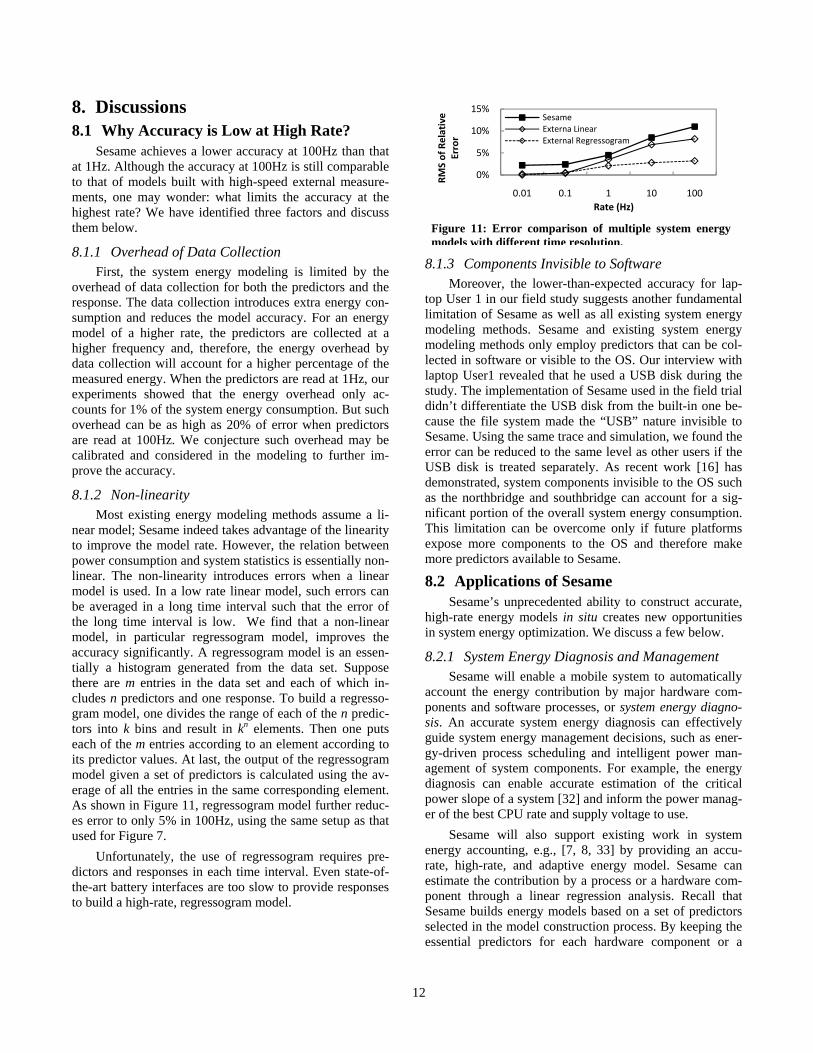
8.1.2 Non-linearity Most existing energy modeling methods assume a li-

near model; Sesame indeed takes advantage of the linearity to improve the model rate. However, the relation between power consumption and system statistics is essentially non-linear. The non-linearity introduces errors when a linear model is used. In a low rate linear model, such errors can be averaged in a long time interval such that the error of the long time interval is low. We find that a non-linear model, in particular regressogram model, improves the accuracy significantly. A regressogram model is an essen-tially a histogram generated from the data set. Suppose there are m entries in the data set and each of which in-cludes n predictors and one response. To build a regresso-gram model, one divides the range of each of the n predic-tors into k bins and result in kn elements. Then one puts each of the m entries according to an element according to its predictor values. At last, the output of the regressogram model given a set of predictors is calculated using the av-erage of all the entries in the same corresponding element. As shown in Figure 11, regressogram model further reduc-es error to only 5% in 100Hz, using the same setup as that used for Figure 7.

Unfortunately, the use of regressogram requires pre-dictors and responses in each time interval. Even state-of-the-art battery interfaces are too slow to provide responses to build a high-rate, regressogram model.

8.1.3 Components Invisible to Software Moreover, the lower-than-expected accuracy for lap-

top User 1 in our field study suggests another fundamental limitation of Sesame as well as all existing system energy modeling methods. Sesame and existing system energy modeling methods only employ predictors that can be col-lected in software or visible to the OS. Our interview with laptop User1 revealed that he used a USB disk during the study. The implementation of Sesame used in the field trial didn’t differentiate the USB disk from the built-in one be-cause the file system made the “USB” nature invisible to Sesame. Using the same trace and simulation, we found the error can be reduced to the same level as other users if the USB disk is treated separately. As recent work [16] has demonstrated, system components invisible to the OS such as the northbridge and southbridge can account for a sig-nificant portion of the overall system energy consumption. This limitation can be overcome only if future platforms expose more components to the OS and therefore make more predictors available to Sesame.

8.2 Applications of Sesame Sesame’s unprecedented ability to construct accurate,

high-rate energy models in situ creates new opportunities in system energy optimization. We discuss a few below.

8.2.1 System Energy Diagnosis and Management Sesame will enable a mobile system to automatically

account the energy contribution by major hardware com-ponents and software processes, or system energy diagno-sis. An accurate system energy diagnosis can effectively guide system energy management decisions, such as ener-gy-driven process scheduling and intelligent power man-agement of system components. For example, the energy diagnosis can enable accurate estimation of the critical power slope of a system [32] and inform the power manag-er of the best CPU rate and supply voltage to use.

Sesame will also support existing work in system energy accounting, e.g., [7, 8, 33] by providing an accu-rate, high-rate, and adaptive energy model. Sesame can estimate the contribution by a process or a hardware com-ponent through a linear regression analysis. Recall that Sesame builds energy models based on a set of predictors selected in the model construction process. By keeping the essential predictors for each hardware component or a

Figure 11: Error comparison of multiple system energy models with different time resolution.

0%

5%

10%

15%

0.01 0.1 1 10 100

RMS of Relative

 Error

Rate (Hz)

SesameExterna LinearExternal Regressogram

13

group of hardware components, Sesame can construct a model in which the sum of products of the predictors and their coefficient represents the energy contribution of the corresponding hardware component.

Sesame can account energy by process using OS-reported account of each process’s contribution to the val-ue of a predictor. For example, the OS reports CPU P-state residency as contributed by an individual process. Thus, the product of each predictor and its coefficient in the li-near model can be further broken down into contributions from multiple processes through the corresponding hard-ware component associated with the predictor.

8.2.2 Software Energy Optimization Sesame can be also used to drive software energy op-

timization with energy models constructed through real usage by taking predictors from an individual application. Many software applications provide tunable variables or “knobs” to provide different qualities of services, either as inherent parameters for energy-aware adaptation, e.g., [34], or as variables selected by the developers for tuning the software for energy efficiency. The challenge to using such “knobs” lies in the difficulty to quantify their impact on system energy because the efficiency of an application is highly dependent on the system configuration and usage. An energy model based on such knobs are necessary [9, 35]. Sesame can readily solve this problem by incorporat-ing such knobs as predictors in its energy construction to build an application-specific energy model only using the application knobs and therefore estimate the connections between them and the system energy directly. Because such estimations provide quantitative information regard-ing the energy savings by turning different knobs, the ap-plication can be adapted in situ either automatically by itself or by the user to effectively make tradeoffs between quality of service and efficiency.

9. Conclusions In this work, we demonstrated the feasibility of self-

energy modeling of mobile systems, or Sesame, with which a mobile system constructs an energy model of itself without any external assistance. We reported a Linux-based prototype of Sesame and showed it achieves 95% accuracy for laptop (T61) and 86% for smartphone (N900) with a rate of 1Hz, which is comparable to existing system energy models built in lab with the help of a second com-puter. Moreover, Sesame is able to achieve 88% and 82% accuracy for T61 and N900, respectively, at 100Hz, which is at least 100 times faster than existing system energy models. Our field study with four laptop users and four smartphone users further attested to Sesame’s effectiveness and noninvasiveness. The high accuracy and high rate of system energy models built by Sesame allows for innova-tive applications of system energy models, e.g., energy-aware scheduling, rogue application detection, and incen-

tive mechanisms for participatory sensing, on a multitask-ing mobile system.

Finally, although Sesame was originally intended for mobile systems, the self-modeling approach is readily ap-plicable to other systems with self power measurement capability, e.g., servers powered by a power supply unit with a power meter. The overhead reduction and accura-cy/rate improvement techniques of Sesame will be instru-mental.

10. References [1] H. Kim, J. Smith, and K. Shin, "Detecting energy-greedy

anomalies and mobile malware variants," in Proc. ACM/USENIX Int. Conf. Mobile Systems, Applications, and Services (MobiSys) Breckenridge, CO, USA, 2008.

[2] S. Reddy, D. Estrin, and M. Srivastava, "Recruitment framework for participatory sensing data collections," Per-vasive Computing, pp. 138-155, 2010.

[3] J. Burke, D. Estrin, M. Hansen, A. Parker, N. Ramanathan, S. Reddy, and M. Srivastava, "Participatory sensing," in Workshop on World-Sensor-Web (WSW), 2006.

[4] K. J. R. Liu, A. K. Sadek, W. Su, and A. Kwasinski, Coop-erative Communications and Networking: Cambridge Uni-versity Press, 2009.

[5] M. Anand, E. B. Nightingale, and J. Flinn, "Ghosts in the machine: interfaces for better power management," in Proc. ACM/USENIX Int. Conf. Mobile Systems, Applications, and Services (MobiSys) Boston, MA, USA, 2004.

[6] F. Bellosa, A. Weissel, M. Waitz, and S. Kellner, "Event-driven energy accounting for dynamic thermal manage-ment," in Proc. Workshop on Compilers and Operating Sys-tems for Low Power (COLP'03) New Orleans, Louisiana, USA, 2003.

[7] R. Neugebauer and D. McAuley, "Energy is just another resource: energy accounting and energy pricing in the Ne-mesis OS," in Proc. Workshop on Hot Topics in Operating Systems (HotOS-VIII) Oberbayern, Germany, 2001.

[8] H. Zeng, C. S. Ellis, A. R. Lebeck, and A. Vahdat, "ECO-System: managing energy as a first class operating system resource," in Proc Int. Conf. Architectural Support for Pro-gramming Languages and Operating Systems (ASPLOS-X) San Jose, CA, USA, 2002.

[9] J. Flinn and M. Satyanarayanan, "Energy-aware adaptation for mobile applications," in Proc. ACM Symp. Operating Systems Principles (SOSP) Charleston, SC, USA, 1999.

[10] P. Dutta, M. Feldmeier, J. Paradiso, and D. Culler, "Energy Metering for Free: Augmenting Switching Regulators for Real-Time Monitoring," in Proc. Int. Conf. Information Processing in Sensor Networks (IPSN) St. Louis , MO , USA, 2008.

[11] R. Fonseca, P. Dutta, P. Levis, I. Stoica, C. A. Berkeley, and C. A. Stanford, "Quanto: Tracking energy in networked em-bedded systems," in Proc. Symp. Operating System Design and Implementation (OSDI), 2008, pp. 323–338.

[12] A. Kansal, F. Zhao, J. Liu, N. Kothari, A. Bhattacharya, and N. Computing, "Virtual Machine Power Metering and Provi-sioning," in Proc. ACM Symposium on Cloud Computing, 2010.

[13] J. S. Chase, D. C. Anderson, P. N. Thakar, A. M. Vahdat, and R. P. Doyle, "Managing energy and server resources in

14

hosting centers," in Proc. ACM Symp. Operating Systems Principles (SOSP) Banff, Alberta, Canada, 2001.

[14] T. L. Cignetti, K. Komarov, and C. S. Ellis, "Energy estima-tion tools for the Palm," in Proc. ACM Int. Workshop on Modeling, Analysis and Simulation of Wireless and Mobile Systems (MSWiM'00) Boston, MA, USA, 2000.

[15] M. Anand, E. B. Nightingale, and J. Flinn, "Self-tuning wireless network power management," in Proc. ACM Int. Conf. Mobile Computing and Networking (MobiCom) San Diego, CA, USA, 2003.

[16] R. Muralidhar, H. Seshadri, K. Paul, and S. Karumuri, "Li-nux-based Ultra Mobile PCs," in Proceedings of Linux Sym-posium Ottawa, Canada, 2007.

[17] PowerTutor, "http://powertutor.org/." [18] A. Shye, B. Scholbrock, and G. Memik, "Into the wild: stud-

ying real user activity patterns to guide power optimizations for mobile architectures," in Proc. IEEE/ACM Int. Symp. Microarchitecture (MICRO-42) New York, New York, USA, 2009.

[19] X. Fan, W. Weber, and L. Barroso, "Power provisioning for a warehouse-sized computer," in Proc. Int. Symp. Computer Architecture (ISCA) San Diego, CA, USA, 2007.

[20] D. Economou, S. Rivoire, C. Kozyrakis, and P. Rangana-than, "Full-system power analysis and modeling for server environments," in Proc. Workshop on Modeling Benchmark-ing and Simulation (MOBS'06) Boston, MA, USA, 2006.

[21] D. Brooks, V. Tiwari, and M. Martonosi, "Wattch: a frame-work for architectural-level power analysis and optimiza-tions," in Proc. Int. Symp. Computer Architecture (ISCA) Vancouver, British Columbia, Canada, 2000.

[22] G. Contreras and M. Martonosi, "Power prediction for intel XScale processors using performance monitoring unit events," in Proc. ACM/IEEE Int. Symp. Low Power Elec-tronics and Design (ISLPED) San Diego, CA, USA, 2005.

[23] F. Rawson, "MEMPOWER: A Simple Memory Power Analysis Tool Set," IBM Austin Research Laboratory2004.

[24] P. Ranganathan and P. Leech, "Simulating complex enter-prise workloads using utilization traces," 2007.

[25] BLTK, "http://www.lesswatts.org/projects/bltk/." [26] H. Falaki, R. Mahajan, S. Kandula, D. Lymberopoulos, R.

Govindan, and D. Estrin, "Diversity in Smartphone Usage," in Proc. ACM Int. Conf. Mobile Systems, Applications, and Services (MobiSys) San Francisco, CA, 2010.

[27] A. Rahmati and L. Zhong, "A longitudinal study of non-voice mobile phone usage by teens from an underserved ur-ban community," Technical Report 0515-09, Rice Universi-ty, 2009.

[28] SBS, "http://smartbattery.org/." [29] Texas Instruments, "SBS-Complaint Gas Gauge IC Use

With The bq29311," 2002. [30] S. V. Huffel and P. Lemmerling, Total Least Squares and

Errors-in-Variables Modeling: Analysis, Algorithms and Applications: Dordrecht, The Netherlands: Kluwer Academ-ic Publishers, 2002.

[31] GSL, "http://www.gnu.org/software/gsl/." [32] A. Miyoshi, C. Lefurgy, E. V. Hensbergen, R. Rajamony,

and R. Rajkumar, "Critical power slope: understanding the runtime effects of frequency scaling," in Proceedings of the 16th international conference on Supercomputing New York, New York, USA: ACM, 2002.

[33] F. Bellosa, "The benefits of event-driven energy accounting in power-sensitive systems," in Proceedings of the 9th work-

shop on ACM SIGOPS European workshop: beyond the PC: new challenges for the operating system Kolding, Denmark, 2000.

[34] J. Flinn and M. Satyanarayanan, "Energy-aware adaptation for mobile applications," SIGOPS Oper. Syst. Rev., vol. 33, pp. 48-63, 1999.

[35] J. Lorch and A. Smith, "Software strategies for portable computer energy management," IEEE Personal Communica-tions, vol. 5, pp. 60-73, June 1998.

Appendix: Invariance of Linear Models

The key technique employed by Sesame to overcome the accuracy and rate limitations of battery interfaces is model molding, which first builds a linear energy model for long time intervals and then uses the same model for much shorter intervals. See Section 5.3.1. Model molding fun-damentally assumes that the liner energy model is invariant at different time scales. That is, it assumes the coefficient vector of the linear model, | , is the same for T of different lengths.

We next provide the physical rationale behind this heuristics. Suppose a system includes components, the th component has states, 1,2, … , the th compo-

nent in the th state consumes power , 1,2, … ,

1,2, … , . Let denote the time the th component spends in the th state during the time interval of T. The energy consumption of the system during the interval can be there-fore calculated as

∑ ∑ ,

which is essentially a linear function of . When we divide the time interval from both sides, we have

/ ∑ ∑ / .

Now if we use / , the ratio of time that the th com-ponent spends in the th state, as predictors, the average power consumption of the system, / , can be calculated using the same no matter what time scale T is in. Because it is impractical to obtain / for all compo-nents and their states, practical energy models have to use system statistics as used in this work. Such system statis-tics cover major power consumers in the system and they are usually highly related to / , e.g., CPU utilization, but they usually involve the activities of multiple components and thus are correlated with each other. Therefore, the use of PCA can minimize the correlation among the system statistics and generate a new set of predictors independent with each other and closer to / . The invariance of will largely hold for a linear model built with the new pre-dictors generated by PCA.