sesam user manual wadam - høgskulen på vestlandethome.hib.no/ansatte/tct/ftp/h2017 marinteknisk...
TRANSCRIPT

SESAM USER MANUAL
WADAMWave Analysis by Diffraction and Morison theory
Valid from program version 9.3
SAFER, SMARTER, GREENER

Sesam User Manual
Wadam
Date: March/2017
Valid from program version 9.3
Prepared by DNV GL - Software
E-mail support: [email protected]
E-mail sales: [email protected]
c©DNV GL AS. All rights reserved
This publication or parts thereof may not be reproduced or transmitted in any form or by any means, including copying
or recording, without the prior written consent of DNV GL AS.

Table of contents
1 INTRODUCTION . . . . . . . . . . . . . . . . . . . . . . . . . . . . . . . . . . . . . . . . . . . . . 21.1 Wadam – Wave Analysis by Diffraction and Morison Theory . . . . . . . . . . . . . . . . . . . . . 21.2 Wadam in the Sesam system . . . . . . . . . . . . . . . . . . . . . . . . . . . . . . . . . . . . . . 31.3 How to Read this Manual . . . . . . . . . . . . . . . . . . . . . . . . . . . . . . . . . . . . . . . . 31.4 Terminology and Notation . . . . . . . . . . . . . . . . . . . . . . . . . . . . . . . . . . . . . . . 41.5 Status List . . . . . . . . . . . . . . . . . . . . . . . . . . . . . . . . . . . . . . . . . . . . . . . . 41.6 Wadam Extensions . . . . . . . . . . . . . . . . . . . . . . . . . . . . . . . . . . . . . . . . . . . 5
2 FEATURES OF WADAM . . . . . . . . . . . . . . . . . . . . . . . . . . . . . . . . . . . . . . . . . 62.1 Definition of Model Types in Wadam . . . . . . . . . . . . . . . . . . . . . . . . . . . . . . . . . . 62.1.1 The Coordinate Systems . . . . . . . . . . . . . . . . . . . . . . . . . . . . . . . . . . . . . . . . 72.1.2 The Panel Model . . . . . . . . . . . . . . . . . . . . . . . . . . . . . . . . . . . . . . . . . . . . 92.1.3 The Morison Model . . . . . . . . . . . . . . . . . . . . . . . . . . . . . . . . . . . . . . . . . . . 102.1.4 The Composite Model . . . . . . . . . . . . . . . . . . . . . . . . . . . . . . . . . . . . . . . . . 162.1.5 Single Super element Composite model . . . . . . . . . . . . . . . . . . . . . . . . . . . . . . . 172.1.6 Multi-Body Modelling . . . . . . . . . . . . . . . . . . . . . . . . . . . . . . . . . . . . . . . . . . 172.1.7 Mass Modelling . . . . . . . . . . . . . . . . . . . . . . . . . . . . . . . . . . . . . . . . . . . . . 182.1.8 Structural Modelling . . . . . . . . . . . . . . . . . . . . . . . . . . . . . . . . . . . . . . . . . . 192.1.9 Free Surface Modelling . . . . . . . . . . . . . . . . . . . . . . . . . . . . . . . . . . . . . . . . . 202.1.10 Load Case Numbering and Load Case Combinations . . . . . . . . . . . . . . . . . . . . . . . . 20
2.2 Global Response Analysis . . . . . . . . . . . . . . . . . . . . . . . . . . . . . . . . . . . . . . . . 232.2.1 General . . . . . . . . . . . . . . . . . . . . . . . . . . . . . . . . . . . . . . . . . . . . . . . . . 232.2.2 Computation of Wave Loads . . . . . . . . . . . . . . . . . . . . . . . . . . . . . . . . . . . . . . 232.2.3 The Global Response Results . . . . . . . . . . . . . . . . . . . . . . . . . . . . . . . . . . . . . 24
2.3 The Calculation of Detailed Loads on a Structural Model . . . . . . . . . . . . . . . . . . . . . . 242.3.1 General . . . . . . . . . . . . . . . . . . . . . . . . . . . . . . . . . . . . . . . . . . . . . . . . . 242.3.2 The Structural Load Types . . . . . . . . . . . . . . . . . . . . . . . . . . . . . . . . . . . . . . . 242.3.3 Deterministic Loads . . . . . . . . . . . . . . . . . . . . . . . . . . . . . . . . . . . . . . . . . . 252.3.4 Detailed Loads Transfer to a Model with Shell or Solid Elements . . . . . . . . . . . . . . . . . 252.3.5 Detailed Loads Transfer to a Model with Beam Elements . . . . . . . . . . . . . . . . . . . . . . 25
2.4 Environmental Description . . . . . . . . . . . . . . . . . . . . . . . . . . . . . . . . . . . . . . . 252.4.1 Surface Waves . . . . . . . . . . . . . . . . . . . . . . . . . . . . . . . . . . . . . . . . . . . . . 252.4.2 Current Profiles . . . . . . . . . . . . . . . . . . . . . . . . . . . . . . . . . . . . . . . . . . . . . 272.4.3 Water Depth . . . . . . . . . . . . . . . . . . . . . . . . . . . . . . . . . . . . . . . . . . . . . . 27
2.5 Results Types Reported from Wadam . . . . . . . . . . . . . . . . . . . . . . . . . . . . . . . . . 272.5.1 Units . . . . . . . . . . . . . . . . . . . . . . . . . . . . . . . . . . . . . . . . . . . . . . . . . . . 272.5.2 Result Reference Point . . . . . . . . . . . . . . . . . . . . . . . . . . . . . . . . . . . . . . . . . 282.5.3 Dimensioning of Results . . . . . . . . . . . . . . . . . . . . . . . . . . . . . . . . . . . . . . . . 282.5.4 Transfer Functions and Phase Definitions . . . . . . . . . . . . . . . . . . . . . . . . . . . . . . 292.5.5 Hydrostatic Results . . . . . . . . . . . . . . . . . . . . . . . . . . . . . . . . . . . . . . . . . . . 302.5.6 Global Mass Matrix . . . . . . . . . . . . . . . . . . . . . . . . . . . . . . . . . . . . . . . . . . . 302.5.7 Added Mass Matrix . . . . . . . . . . . . . . . . . . . . . . . . . . . . . . . . . . . . . . . . . . . 312.5.8 Damping Matrix . . . . . . . . . . . . . . . . . . . . . . . . . . . . . . . . . . . . . . . . . . . . 312.5.9 Exciting Forces and Moments . . . . . . . . . . . . . . . . . . . . . . . . . . . . . . . . . . . . . 312.5.10 Rigid Body Motion . . . . . . . . . . . . . . . . . . . . . . . . . . . . . . . . . . . . . . . . . . . 322.5.11 Second Order Mean Drift Forces . . . . . . . . . . . . . . . . . . . . . . . . . . . . . . . . . . . 322.5.12 Second Order Sum and Difference Frequency Results . . . . . . . . . . . . . . . . . . . . . . . 322.5.13 Fluid Kinematics . . . . . . . . . . . . . . . . . . . . . . . . . . . . . . . . . . . . . . . . . . . . 322.5.14 Wave Drift Damping . . . . . . . . . . . . . . . . . . . . . . . . . . . . . . . . . . . . . . . . . . 322.5.15 Distributed Hydrostatic Loads . . . . . . . . . . . . . . . . . . . . . . . . . . . . . . . . . . . . . 332.5.16 Distributed Hydrodynamic Loads . . . . . . . . . . . . . . . . . . . . . . . . . . . . . . . . . . . 332.5.17 Load Sum Reports . . . . . . . . . . . . . . . . . . . . . . . . . . . . . . . . . . . . . . . . . . . 342.5.18 Sectional Loads . . . . . . . . . . . . . . . . . . . . . . . . . . . . . . . . . . . . . . . . . . . . . 352.5.19 Roll Damping Coefficients . . . . . . . . . . . . . . . . . . . . . . . . . . . . . . . . . . . . . . . 362.5.20 Global drag-coefficient for roll-damping . . . . . . . . . . . . . . . . . . . . . . . . . . . . . . . 37
2.6 Calculation Methods . . . . . . . . . . . . . . . . . . . . . . . . . . . . . . . . . . . . . . . . . . . 372.6.1 Calculation of Wave Loads from Potential Theory . . . . . . . . . . . . . . . . . . . . . . . . . . 37
|Sesam User Manual|Wadam|[92-7052] www.dnvgl.com/software Page i

2.6.2 Calculation of Wave Loads from Second Order Potential Theory . . . . . . . . . . . . . . . . . . 382.6.3 Removal of Irregular Frequencies . . . . . . . . . . . . . . . . . . . . . . . . . . . . . . . . . . . 392.6.4 Damping free surface lid . . . . . . . . . . . . . . . . . . . . . . . . . . . . . . . . . . . . . . . 392.6.5 The Equation of Motion . . . . . . . . . . . . . . . . . . . . . . . . . . . . . . . . . . . . . . . . 402.6.6 Morison’s Equation . . . . . . . . . . . . . . . . . . . . . . . . . . . . . . . . . . . . . . . . . . . 402.6.7 Calculation of Tank Pressures, Quasi-static Method . . . . . . . . . . . . . . . . . . . . . . . . . 412.6.8 Calculation of Tank Pressures, Full Dynamic Method . . . . . . . . . . . . . . . . . . . . . . . . 422.6.9 Pressure Loads up to Free Surface . . . . . . . . . . . . . . . . . . . . . . . . . . . . . . . . . . 432.6.10 Reduced pressure up to the free surface . . . . . . . . . . . . . . . . . . . . . . . . . . . . . . . 432.6.11 Wave-current interaction . . . . . . . . . . . . . . . . . . . . . . . . . . . . . . . . . . . . . . . 44
2.7 The Save-Restart System . . . . . . . . . . . . . . . . . . . . . . . . . . . . . . . . . . . . . . . . 44
3 USER’S GUIDE TO WADAM . . . . . . . . . . . . . . . . . . . . . . . . . . . . . . . . . . . . . . 453.1 Column-stabilized Unit . . . . . . . . . . . . . . . . . . . . . . . . . . . . . . . . . . . . . . . . . 453.2 Global Response for a Ship . . . . . . . . . . . . . . . . . . . . . . . . . . . . . . . . . . . . . . . 493.3 Handling of fluid compartments . . . . . . . . . . . . . . . . . . . . . . . . . . . . . . . . . . . . 523.4 Free surface lids . . . . . . . . . . . . . . . . . . . . . . . . . . . . . . . . . . . . . . . . . . . . . 53
4 EXECUTION OF WADAM . . . . . . . . . . . . . . . . . . . . . . . . . . . . . . . . . . . . . . . . 564.1 Program Environment . . . . . . . . . . . . . . . . . . . . . . . . . . . . . . . . . . . . . . . . . . 564.1.1 The Input Files . . . . . . . . . . . . . . . . . . . . . . . . . . . . . . . . . . . . . . . . . . . . . 564.1.2 Output Files . . . . . . . . . . . . . . . . . . . . . . . . . . . . . . . . . . . . . . . . . . . . . . . 584.1.3 The Save-Restart File . . . . . . . . . . . . . . . . . . . . . . . . . . . . . . . . . . . . . . . . . 58
4.2 Processor dependent optimization . . . . . . . . . . . . . . . . . . . . . . . . . . . . . . . . . . . 584.3 Program Requirements . . . . . . . . . . . . . . . . . . . . . . . . . . . . . . . . . . . . . . . . . 594.4 Program Limitations . . . . . . . . . . . . . . . . . . . . . . . . . . . . . . . . . . . . . . . . . . . 594.5 Warnings and Error Messages . . . . . . . . . . . . . . . . . . . . . . . . . . . . . . . . . . . . . 59
Appendices . . . . . . . . . . . . . . . . . . . . . . . . . . . . . . . . . . . . . . . . . . . . . . . . . . . . .
A THEORY . . . . . . . . . . . . . . . . . . . . . . . . . . . . . . . . . . . . . . . . . . . . . . . . . . A1A 1 Hydrostatic Forces . . . . . . . . . . . . . . . . . . . . . . . . . . . . . . . . . . . . . . . . . . . . A1A 1.1 Hydrostatic Coefficients . . . . . . . . . . . . . . . . . . . . . . . . . . . . . . . . . . . . . . . . A1
A 2 Morison Element Formulations . . . . . . . . . . . . . . . . . . . . . . . . . . . . . . . . . . . . . A1A 2.1 The Anchor Element Formulation . . . . . . . . . . . . . . . . . . . . . . . . . . . . . . . . . . . A2A 2.2 The TLP Mooring Element Formulation . . . . . . . . . . . . . . . . . . . . . . . . . . . . . . . . A2
A 3 Calculation Methods . . . . . . . . . . . . . . . . . . . . . . . . . . . . . . . . . . . . . . . . . . . A3A 3.1 Linearisation of Roll Restoring . . . . . . . . . . . . . . . . . . . . . . . . . . . . . . . . . . . . . A3A 3.2 Calculation of Line Loads . . . . . . . . . . . . . . . . . . . . . . . . . . . . . . . . . . . . . . . A4A 3.3 The Mapping of Loads from Panel Models to Finite Element Models . . . . . . . . . . . . . . . . A5A 3.4 Calculation of Tank Pressures . . . . . . . . . . . . . . . . . . . . . . . . . . . . . . . . . . . . . A6A 3.5 Global drag-coefficient for roll . . . . . . . . . . . . . . . . . . . . . . . . . . . . . . . . . . . . . A7
B The Wadam Print File List of Contents . . . . . . . . . . . . . . . . . . . . . . . . . . . . . . B1
References . . . . . . . . . . . . . . . . . . . . . . . . . . . . . . . . . . . . . . . . . . . . . . . . . . . . .
|Sesam User Manual|Wadam|[92-7052] www.dnvgl.com/software Page 1

1 INTRODUCTION
1.1 Wadam – Wave Analysis by Diffraction and Morison Theory
Wadam is a general analysis program for calculation of wave-structure interaction for fixed and floatingstructures of arbitrary shape, e.g. semi-submersible platforms, tension-leg platforms, gravity-base struc-tures and ship hulls.
The analysis capabilities in Wadam comprise:
• Calculation of hydrostatic data and inertia properties
• Calculation of global responses including:
– First and second order wave exciting forces and moments
– Hydrodynamic added mass and damping
– First and second order rigid body motions
– Sectional forces and moments
– Steady drift forces and moments
– Wave drift damping coefficients
– Internal tank pressures
• Calculation of selected global responses of a multi-body system
• Automatic load transfer to a finite element model for subsequent structural analysis including:
– Inertia loads
– Line loads for structural beam element analysis
– Pressure loads for structural shell/solid element analysis
– Pressure loads up to the free surface
Wadam calculates loads using:
• Morison’s equation for slender structures
• First and second order 3D potential theory for large volume structures
• Morison’s equation and potential theory when the structure comprises of both slender and largevolume parts. The forces at the slender part may optionally be calculated using the diffracted wavekinematics calculated from the presence of the large volume part of the structure.
The Wadam results may be presented directly as complex transfer functions or converted to time domainresults for a specified sequence of phase angles of the incident wave. For fixed structures Morison’s equa-tion may also be used with a time domain output option to calculate drag forces due to time independentcurrent.
The same analysis model may be applied to both the calculation of global responses in Wadam and thesubsequent structural analysis. For shell and solid element models Wadam also provides automatic mappingof pressure loads from a panel model to a differently meshed structural finite element model.
The 3D potential theory in Wadam is based directly on the Wamit program developed by MassachusettsInstitute of Technology Ref. [1] and Ref. [2].
|Sesam User Manual|Wadam|[92-7052] www.dnvgl.com/software Page 2

1.2 Wadam in the Sesam system
Wadam is an integrated part of the Sesam suite of programs. It is tailored to calculate wave loads on modelscreated by the Sesam preprocessors Patran-Pre, Prefem, GeniE and Presel. The models are read by Wadamfrom the Input Interface File (T-file). The Wadam analysis control data is generated by the Hydrodynamicdesign tool HydroD.
The results from the Wadam global response analysis may be stored on a Hydrodynamic Results InterfaceFile (G-file) for statistical postprocessing in Postresp. The loads mapped to structural finite elements may bestored on the Loads Interface File (L-file) for a subsequent structural analysis in Sestra.
Figure 1.1 shows Wadam in the Sesam system. A detailed description of the input and output files is givenin Section 4.
Figure 1.1: Sesam overview
1.3 How to Read this Manual
Section 2 FEATURES OF WADAM describes the problems Wadam can solve. Descriptions of models, environ-ment and results produced by Wadam are included.
Section 3 USER’S GUIDE TO WADAM presents tutorial examples. Each example includes a discussion of themodelling, execution and results interpretation phases. Both simple examples and engineering applicationsare included.
Section 4 EXECUTION OF WADAM describes the input and output files of Wadam. The memory and diskstorage requirements are discussed together with some rules of thumb on execution time for different typesof analysis. Finally, the chapter lists the problem size limitations in Wadam.
Appendix A THEORY includes additional theory description for Wadam.
|Sesam User Manual|Wadam|[92-7052] www.dnvgl.com/software Page 3

1.4 Terminology and Notation
Composite model A hydro model consisting of a panel model and Morison model repre-senting separate parts of the structure. See Section 2.1.4.
FE Abbreviation for ’finite-element’ like in FE model.
HydroD The hydrodynamic design tool. This is a modern graphical tool formodelling the input data to Wadam. Wadam is started directly fromwithin this application.
Hydrodynamic Results Interface File A file containing results from a global response analysis. This file istermed G-file for short. The post-processor Postresp performs sta-tistical post-processing of these results. See Section 2.2 and Sec-tion 4.1.2.
Hydro model Hydrodynamic model. A model used for calculating hydrodynamicloads from potential theory and Morison’s equation. See Section 2.1.
Hydro property Hydrodynamic properties including added mass, drag coefficients, el-ement diameters and anchor characteristics required for calculatinghydrodynamic loads.
Input Interface File A file containing geometrical information of the structure (FE modelplus hydro model). This file is termed T-file for short. See Sec-tion 4.1.1.
Loads Interface File A file containing loads for a subsequent structural analysis. This fileis termed L-file for short. See Section 4.1.2.
Prewad Was Wadam’s interactive preprocessor. This has now been removed.
RSQ File Wadam’s save-restart file <user-defined name>.RSQ; see Section 2.7and Section 4.1.3.
S-file A file containing information on the relation between load cases andwave frequencies. See Section 2.3.
swl Abbreviation for ’still water level’.
1.5 Status List
There exists for Wadam (as for all other Sesam programs) a Status List providing additional information. Thismay be:
• Reasons for update (new version)
• New features
• Errors found and corrected
• Etc.
The most recently updated status lists can be accessed over the internet. Go to www.dnvgl.com/softwareand select the Support link. Then log in to the Customer portal for Sesam. A user name and password isrequired to access this site. Please follow the instructions given to obtain access.
In the Status List Browser window narrow the number of entries listed:
• Entries relevant to a specific version only
• Entries of a specific type, e.g. Reasons-for-Update
• Entries containing a given text string
|Sesam User Manual|Wadam|[92-7052] www.dnvgl.com/software Page 4

1.6 Wadam Extensions
Wadam has the following extensions which require separate license keys:
2ORD Calculation of second order sum- and difference- frequency transfer functions for bodies inmonochromatic and bi-chromatic incident waves.
NBOD Calculation of first-order hydrodynamic analysis of multiple bodies.
STRU Transfer of hydrodynamic loads to structural finite element models with beam, shell and solid ele-ments.
WDD Computation of Wave Drift damping coefficients.
|Sesam User Manual|Wadam|[92-7052] www.dnvgl.com/software Page 5

2 FEATURES OF WADAM
This section describes the features of the Wadam program. The section is organised with Section 2.1 de-scribing the modelling concepts adopted in Wadam. Thereafter, Section 2.2 and Section 2.3 describe thetwo main analysis capabilities:
• Global response analysis for calculating rigid body type of results.
• Detailed load calculation for transfers of finite element type of loads to a structural model.
The environmental definition including both surface waves and current profiles is introduced in Section 2.4.The description of the results produced by Wadam is included in Section 2.5. Basic calculation methods aredescribed in Section 2.6. Additional information on calculation methods is included in Appendix A.
2.1 Definition of Model Types in Wadam
The definition of models in Wadam includes three main model types: (1) the hydro model which is used tocalculate hydrodynamic forces, (2) the structural model where hydrodynamic and hydrostatic loads are rep-resented as finite element loads and (3) the mass model. The mass model is relevant for floating structuresonly and may be defined as finite elements with mass properties or as a global mass matrix. Alternatively,the distributed mass points specified in a file can be given as input to the mass model from HydroD. Thedifferent model types, see Figure 2.1, are described in this section. Wadam reads the various models fromInput Interface Files generated by e.g. the Sesam preprocessors GeniE, Patran-Pre and Presel.
Figure 2.1: Overview of model types in Wadam
The hydro model may, see Figure 2.1, consist of either:
• A panel model for calculation of hydrodynamic results from potential theory
• A Morison model for calculation of hydrodynamic loads from Morison’s equation
• A combination of a panel- and a Morison model – called a composite model. The composite model isused when potential theory and Morison’s equation are applied to different parts of the hydro model.
The legal combinations of panel and Morison models are shown in Figure 2.2.
The element types interpreted by Wadam are listed in Table 2.1. Other element types present in the variousWadam models will be neglected.
|Sesam User Manual|Wadam|[92-7052] www.dnvgl.com/software Page 6

Figure 2.2: Hydro model combinations
Table 2.1: Overview of Sesam element types interpreted in the various Wadam models
Type of elementNumberof nodes
Panelmodel
Morisonmodel
Massmodel
Structuralmodel
Beam elements
Beam 2 v v v
Curved beam 3 v v
Shell elements
Triangular flat thin shell 3 v v v
Quadrilateral flat thin shell 4 v v v
Subparametric curved triangular thick shell 6 v v v
Subparametric curved quadrilateral thick shell 8 v v v
Multilayered curved triangular shell 6 v v v
Multilayered curved quadrilateral shell 8 v v v
Solid elements
Triangular prism 6 v v v
Linear hexahedron 8 v v v
Tetrahedron 4 v v v
Isoparametric triangular prism 15 v v v
Isoparametric hexahedron 20 v v v
Isoparametric tetrahedron 10 v v v
Mass elements
One node mass element 1 v v v
2.1.1 The Coordinate Systems
Wadam uses three different coordinate systems for single-body hydro models:
• A global coordinate system
• An input coordinate system
• Local finite element coordinate systems
For multi-body hydro models a more general definition applies to the coordinate systems; see Section 2.1.6.
|Sesam User Manual|Wadam|[92-7052] www.dnvgl.com/software Page 7

The global coordinate system, denoted (Xglo, Yglo, Zglo), is right handed with the origin in the still water level.The Z-axis is normal to the still water level and the positive Z-axis is pointing upwards as shown in theFigure 2.3 and Figure 2.4. By default, the results refer to the global coordinate system. The origin is termedthe results reference point or the motion reference point. It is also possible, for the user, to specify anotherresult reference point.
Figure 2.3: 2D representation of a TLP hull with input coordinate system below the swl
Figure 2.4: 2D representation of a semi-submersible with centre of gravity along the globalz-axis
The input coordinate system, denoted (xinp, yinp, zinp), is the coordinate system in which the hydro modeland the structural model are defined. Wadam imposes the restriction that all input models, i.e. the panel,Morison, mass and FE models must be modelled with the same input coordinate system. The coordinates ofthe off-body points are given in the global coordinate system in HydroD.
If the Hydrodynamic preprocessor HydroD is used, there are no constraints on the position or orientation ofthe input coordinate system. The input coordinate system is specified in relation to the global coordinatesystem by 3 translations and 3 Euler angles.
Local finite element coordinate systems are also used in the hydro model when this includes a Morisonmodel. These local coordinate systems are discussed in the sections where they are referred to.
|Sesam User Manual|Wadam|[92-7052] www.dnvgl.com/software Page 8

2.1.2 The Panel Model
The panel model is used to calculate the hydrodynamic loads and responses from potential theory.
The panel model may be a single superelement or a hierarchy of superelements. It may describe either theentire wet surface or it may take advantage of either one or two planes of symmetry of the wet surface.With symmetry planes employed the computational effort to solve the potential problem is reduced bothwith respect to CPU and disk space resources. When the panel model includes more than one body, seeSection 2.1.6, there is the restriction that no planes of symmetry can be exploited.
The symmetry plane option requires that the basic part, i.e. the actually modelled part, is modelled onthe positive side of the symmetry planes as shown in Figure 2.5. Figure 2.6 also shows the basic part of aTension Leg Platform (TLP) panel model.
Note: No panels are allowed in the symmetry plane(s).
Figure 2.5: Symmetry plane definitions
Figure 2.6: The basic part of a TLP panel model
The basic part of a panel model consists of quadrilateral or triangular panels representing the wet surfacesof a body. The panel model can be modelled in GeniE or Patran-Pre using standard finite elements, or withinHydroD from a section model. If more than one superelement is modelled the superelements must beassembled in Presel. The elements accepted in the panel model are defined in Table 2.1.
Note that panels are constructed by drawing straight line segments between the corner nodes of the finiteelement sides. Twisted panels are then forced to be planar by projecting element corner nodes onto panelvertices in the plane defined by the line segment midpoints. The plane of the panel is defined by a pointbeing the mean of the element corner points and a normal vector being the cross product of the directionalvectors of the lines between the straight edge midpoints.
The wet surface of a panel model is identified by defining a dummy load on the panel model in GeniE orPatran-Pre by applying a so-called HYDRO-PRESSURE load with load case number one to all external wetsurfaces of the model. Panels will be generated for all element sides below the still water level and abovethe sea bed where HYDRO-PRESSURE load is defined. The model may be verified in HydroD by displaying
|Sesam User Manual|Wadam|[92-7052] www.dnvgl.com/software Page 9

the mesh with dummy hydro pressure illustrated by arrows pointing from the fluid onto the wet elementsides. In Patran-Pre the corresponding option is the Hydro, Element Uniform load.
Wadam will automatically adjust the wet element sides extending above the still water level into panels withits uppermost edge and vertices in the still water level. Depending on the shape and orientation of the wetelement sides this may actually lead to either an adjustment or a division of a wet element side into newpanels as shown by examples in Figure 2.7. This automatic algorithm is also used to adjust panels extendingbelow the sea-bed.
Figure 2.7: Panel adjustments at the still water level
The Wadam data check reports all the panels extracted from the input panel model noting specifically thosepanels which have been adjusted or divided into two separate panels.
The modelling of a panel model with thick shell elements, which often is the case when the panel model isdefined as the wet surface of a structural model, may introduce significant deviations in the representationof volume and area exposed to wave forces. It may be required to establish a separate panel model withnodes on the outer surface of the thick shell structural model.
From version 9.3 of Wadam, a panel model can be defined on the free surface either in the interior domainfor removal of irregular frequencies or in the exterior domain for assigning of free surface damping. In eitherof these applications, the panel elements on the free surface should be defined as a separated dummy bodyin each domain with the dummy hydro pressure pointing upwards.
The following items should be remembered when modelling a panel model:
• The pressure variation as a function of draught is at a maximum close to the surface, i.e. smallelement heights should be used close to the surface.
• The pressure variation is large close to the edges in the structure, i.e. element sizes normal to theedge length should be small.
• The elements should be modelled as planar as possible. Elements which are too twisted should bedivided into smaller elements.
• Large changes in element size for neighbouring elements should be avoided.
• The largest element diagonal should be smaller than 1/6 of the smallest wave length analysed.This requirement shall also be applied for the free surface lids described in Section 2.6.3 and Sec-tion 2.6.4.
It is also noted that the mesh refinement of a hydro model normally needs to be high if the mean drift forcesby pressure integration shall be obtained. This compared to the calculation of rigid body responses wherereliable results may be obtained with a considerably coarser mesh.
2.1.3 The Morison Model
The Morison model is used to calculate hydrodynamic loads based on Morison’s equation. In addition torepresenting the complete or parts of the structure the Morison model is used to include external forcesfrom mooring lines and tethers in a hydro model.
The Morison model is put together from a set of Morison elements. The Morison elements are based on 2node beam elements and single nodes in a first level superelement generated by Patran-Pre or GeniE. TheMorison elements are actually defined by assigning hydrodynamic properties to nodes and beam elementsin HydroD.
|Sesam User Manual|Wadam|[92-7052] www.dnvgl.com/software Page 10

The different types of Morison elements available for calculation of hydrostatic and hydrodynamic effectsare:
• 2D Morison elements for calculation of hydrostatic and hydrodynamic loads on wet 2 node beamelements
• 3D Morison elements for calculation of hydrostatic and hydrodynamic loads in three directions inspecific nodes
• Pressure area elements for calculation of hydrostatic and hydrodynamic loads at the ends of 2DMorison elements
• Anchor and TLP elements for calculation of additional restoring contributions in specific nodes
Note: The Morison model must be modelled as one single first level superelement. No symme-try plane options are available for the Morison model.
Figure 2.8 shows a beam model and Figure 2.9 the corresponding Morison model representation with 2DMorison elements and pressure area elements. The modelling principles for establishing different types ofMorison elements are discussed in the following subsections.
Figure 2.8: 2 node beam element model of a semi-submersible platform
Figure 2.9: Morison model representation of a semi-submersible platform with 2D Morisonelements and pressure area elements
|Sesam User Manual|Wadam|[92-7052] www.dnvgl.com/software Page 11
2D Morison Elements
A 2D Morison element is defined as a 2 node beam element in a preprocessor and assigned a section numberto be matched by a hydro property section specified in HydroD.
A 2D Morison element is used to include added mass and drag forces according to Morison’s equation; seeSection 2.6.6. It is also used to include hydrostatic restoring contributions.
The hydro property description for a 2D Morison element include added mass and viscous drag coefficientsin the two directions perpendicular to the longitudinal element axis. The hydrodynamic coefficients arespecified in a coordinate system local to each 2D Morison element; see Figure 2.12. In addition, the diameterof the element is specified. The length and diameter may either be taken from the preprocessor generatedbeam model or specified by HydroD.
The section numbers play an important role in the analysis of a Morison model. The use of section numbersto include different hydrodynamic effects in the Morison model should therefore be carefully planned beforesection numbers are assigned to 2D beam elements in the preprocessor. E.g. if different drag and inertiacoefficients shall be used in different locations this should be reflected by the section definitions.
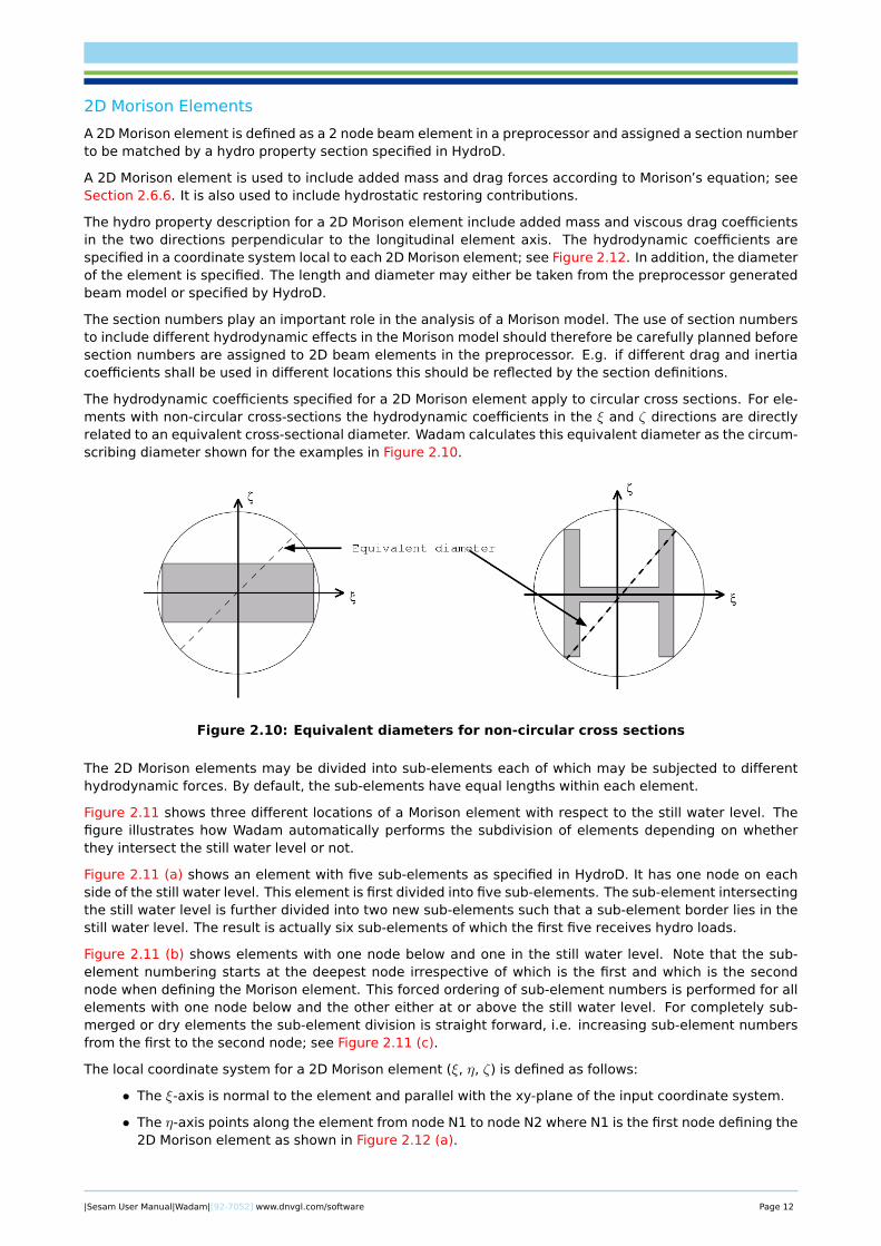
The hydrodynamic coefficients specified for a 2D Morison element apply to circular cross sections. For ele-ments with non-circular cross-sections the hydrodynamic coefficients in the ξ and ζ directions are directlyrelated to an equivalent cross-sectional diameter. Wadam calculates this equivalent diameter as the circum-scribing diameter shown for the examples in Figure 2.10.
Figure 2.10: Equivalent diameters for non-circular cross sections
The 2D Morison elements may be divided into sub-elements each of which may be subjected to differenthydrodynamic forces. By default, the sub-elements have equal lengths within each element.
Figure 2.11 shows three different locations of a Morison element with respect to the still water level. Thefigure illustrates how Wadam automatically performs the subdivision of elements depending on whetherthey intersect the still water level or not.
Figure 2.11 (a) shows an element with five sub-elements as specified in HydroD. It has one node on eachside of the still water level. This element is first divided into five sub-elements. The sub-element intersectingthe still water level is further divided into two new sub-elements such that a sub-element border lies in thestill water level. The result is actually six sub-elements of which the first five receives hydro loads.
Figure 2.11 (b) shows elements with one node below and one in the still water level. Note that the sub-element numbering starts at the deepest node irrespective of which is the first and which is the secondnode when defining the Morison element. This forced ordering of sub-element numbers is performed for allelements with one node below and the other either at or above the still water level. For completely sub-merged or dry elements the sub-element division is straight forward, i.e. increasing sub-element numbersfrom the first to the second node; see Figure 2.11 (c).
The local coordinate system for a 2D Morison element (ξ, η, ζ) is defined as follows:
• The ξ-axis is normal to the element and parallel with the xy-plane of the input coordinate system.
• The η-axis points along the element from node N1 to node N2 where N1 is the first node defining the2D Morison element as shown in Figure 2.12 (a).
|Sesam User Manual|Wadam|[92-7052] www.dnvgl.com/software Page 12

Figure 2.11: The sub-element division of 2D Morison elements
• The ζ-axis is the third axis in the right handed cartesian coordinate system defined by ξ and η.
• The ξ-axis is parallel with the xinp-axis if the η-axis is parallel with the zinp-axis; see Figure 2.12 (b).
3D Morison Elements
A 3D Morison element is defined in HydroD and can only be connected to nodes in the Morison model.
A 3D Morison element may be used to include loads which cannot be represented with a 2D Morison elementin a hydro model. Drag forces and added mass forces in the longitudinal direction of a 2D Morison elementare examples of forces that can be included with a 3D Morison element.
A 3D Morison element may be viewed as a submerged sphere which can receive both hydrostatic andhydrodynamic loads. It will not contribute to the restoring matrix.
The hydro property description for a 3D Morison element includes added mass and viscous drag coefficientsin three directions together with a diameter of the submerged sphere.
The local coordinate system for a 3D Morison element (ξ, η, ζ) will by default coincide with the coordinatesystem of the Morison model (xinp, yinp, zinp). If the local coordinate system shall be different from that ofthe Morison model a guiding point defining the local η-axis must be specified. Figure 2.12 shows this withnode N1 being the 3D Morison element and node N2 being the guiding point. The ξ- and ζ-axes are definedas described above for 2D Morison elements.
The forces on a 3D Morison element is acting at the node to which the 3D Morison element is connected.
|Sesam User Manual|Wadam|[92-7052] www.dnvgl.com/software Page 13
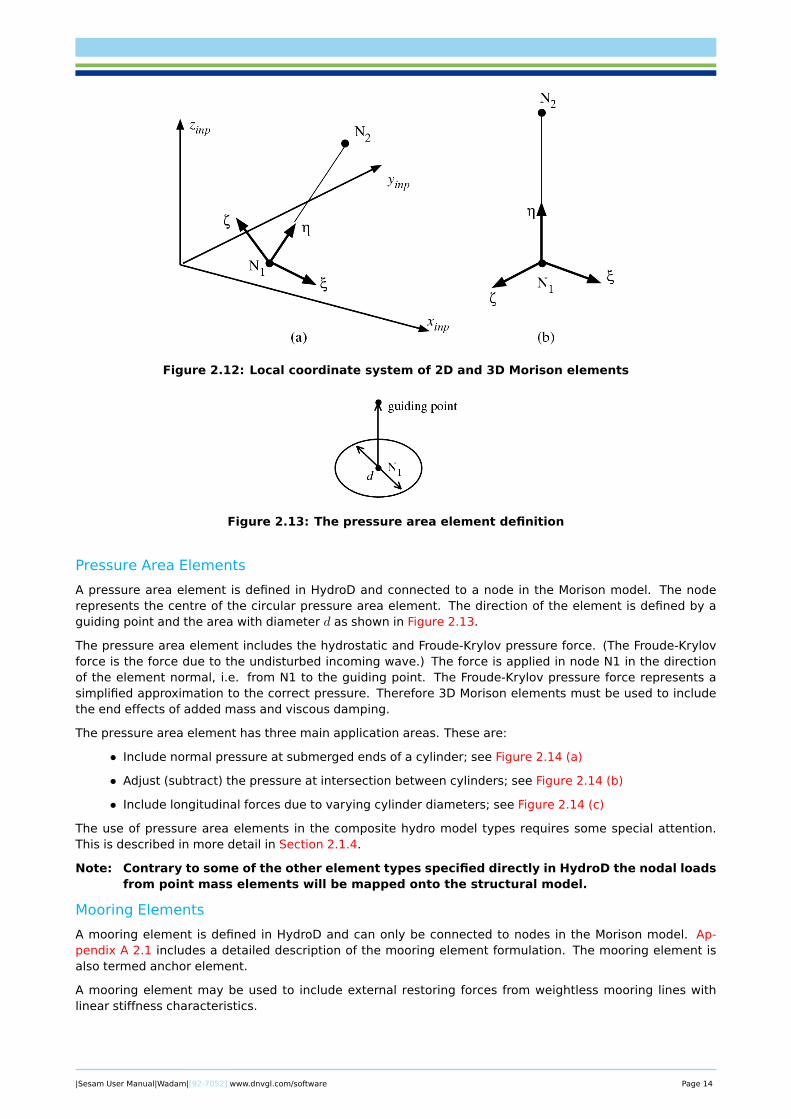
Figure 2.12: Local coordinate system of 2D and 3D Morison elements
Figure 2.13: The pressure area element definition
Pressure Area Elements
A pressure area element is defined in HydroD and connected to a node in the Morison model. The noderepresents the centre of the circular pressure area element. The direction of the element is defined by aguiding point and the area with diameter d as shown in Figure 2.13.
The pressure area element includes the hydrostatic and Froude-Krylov pressure force. (The Froude-Krylovforce is the force due to the undisturbed incoming wave.) The force is applied in node N1 in the directionof the element normal, i.e. from N1 to the guiding point. The Froude-Krylov pressure force represents asimplified approximation to the correct pressure. Therefore 3D Morison elements must be used to includethe end effects of added mass and viscous damping.
The pressure area element has three main application areas. These are:
• Include normal pressure at submerged ends of a cylinder; see Figure 2.14 (a)
• Adjust (subtract) the pressure at intersection between cylinders; see Figure 2.14 (b)
• Include longitudinal forces due to varying cylinder diameters; see Figure 2.14 (c)
The use of pressure area elements in the composite hydro model types requires some special attention.This is described in more detail in Section 2.1.4.
Note: Contrary to some of the other element types specified directly in HydroD the nodal loadsfrom point mass elements will be mapped onto the structural model.
Mooring Elements
A mooring element is defined in HydroD and can only be connected to nodes in the Morison model. Ap-pendix A 2.1 includes a detailed description of the mooring element formulation. The mooring element isalso termed anchor element.
A mooring element may be used to include external restoring forces from weightless mooring lines withlinear stiffness characteristics.
|Sesam User Manual|Wadam|[92-7052] www.dnvgl.com/software Page 14

Figure 2.14: Application areas for the pressure area element
The mooring elements are connected to nodes in the Morison model. The first connection node for themooring element is the guiding point, also termed the fairlead. The second connection point may be at awindlass as shown in Figure 2.15 (a). The two mooring element connections may optionally be the samenode. The hydro properties of a mooring element include the element orientation, the pre-tension and therestoring characteristics.
The element orientation includes two different angles; The angle αinc between the still water level and themooring line and the angle αx between the positive x-axis and the mooring line as shown in Figure 2.15 (b).Note that the angle αinc ≤ π/2 with respect to the negative x-axis for nodes with x < 0.
Figure 2.15: Mooring element definitions
The restoring contributions from the mooring elements are assembled into the body restoring matrix andhence contribute to the rigid body motion. The rigid body motion computed yields dynamic restoring forcesacting in the mooring element nodes. They are mapped onto the structural model as nodal loads. No nodalmoment loads are transferred to the structural model.
Note: Spring elements on the Input Interface File are neglected.
TLP Mooring Elements
A TLP mooring element is defined in HydroD and connected to nodes in the Morison model. It is based on theformulation given in [5]. In addition Appendix A 2.2 summarises the description of the TLP mooring elementformulation.
A TLP mooring element may be used to include external restoring forces from a weightless tether with lineartether characteristics.
|Sesam User Manual|Wadam|[92-7052] www.dnvgl.com/software Page 15

The hydro properties of a TLP mooring element include the length L of the tether, the pre-tension and theelastic stiffness parameter λ. A horizontal offset position xoffset, yoffset may also be specified as shown inFigure 2.16. Note that the tether length shall be the actual length at the offset position.
Figure 2.16: The TLP mooring element
The restoring contributions from the TLP mooring elements are assembled into the body restoring matrix andhence contribute to the rigid body motion. The rigid body motion computed yields dynamic restoring forcesacting in the mooring element nodes. They are mapped onto the structural model as nodal loads.
Note: No nodal moment loads are transferred to the structural model.
2.1.4 The Composite Model
The composite model is a hydro model suitable for structures consisting of both slender and large volumeparts. The slender parts are represented with a Morison model and the large volume parts with a panelmodel.
The hydrodynamic forces on a composite model are computed from potential theory for the panel modeland from Morison’s equation for the Morison model. The hydrodynamic exciting forces and matrices fromboth theories are accumulated in the system of equation of motions for the composite model.
The wave kinematics applied in Morison’s equation may either be taken from the incident wave field. or itmay be specified to depend on the diffracted wave field generated from solving the diffraction problem forthe panel part of the composite model. Figure 2.17 shows a composite model where the risers, modelledwith 2D Morison elements, may optionally be exposed to loads from a diffracted wave field caused by theshaft of the large volume structure.
Figure 2.17: Example of a composite model with a panel model and a non-overlapping Morisonmodel
|Sesam User Manual|Wadam|[92-7052] www.dnvgl.com/software Page 16

With a composite model the pressure area element shall normally be included in the Morison model for allwave lengths.
2.1.5 Single Super element Composite model
From version 8.1-09 of Wadam, the beams receiving loads from the Morison model and the shells or solidsreceiving loads from the panel model may be modelled in the same 1. level super element. The panel modelmay then be defined separately, whereas the Morison model is the same super element as the structuralmodel. It is also possible to have the panel model, the Morison model and the structural model all in thesame super element.
From version 9.1 of Wadam, only the active nodes and elements in the Morison model are taken into account.The accumulation of Morison element for the 2D Morison Section only takes the sections which have beendefined as input. All other elements will be ignored. Moreover, only the nodes which are connected to theeffective Morison elements are counted. With this treatment, it is more practical to use large model asMorison model, especially for the single super element composite model in load transfer analysis.
2.1.6 Multi-Body Modelling
The hydrodynamic and mechanical interaction between a number of structures can be analysed with themulti-body option. The hydrodynamic interaction is computed from the potential theory as applied for asingle structure with the principal extension that the number of degrees of freedom is increased from 6to 6N where N is the number of structures. A stiffness coupling between structures cannot be describeddirectly in Wadam.
Each of the bodies may be represented with a hydro model and optionally a structural model and a massmodel. The bodies may be either fixed or floating.
A hierarchical set of coordinate systems is introduced in which the individual structures and their inputmodels are specified. The coordinate systems applied in a multi-body analysis are therefore different fromthose of a single-body analysis; see Figure 2.18. The coordinate systems are defined as follows:
• The global coordinate system (Xglo, Yglo, Zglo) is a right handed Cartesian coordinate system withits origin at the still water level and with the z-axis normal to the still water level and the positivez-axis pointing upwards.
• The individual body coordinate systems (xB, yB, zB) of each structure are specified relative to theglobal coordinate system.
• The input coordinate system (xinp, yinp, zinp) of each input model included in a body is specifiedrelative to the body coordinate system of that body.
Figure 2.18: The hierarchical coordinate system definition
|Sesam User Manual|Wadam|[92-7052] www.dnvgl.com/software Page 17

The body independent coordinates are described in the global coordinate system, e.g. the fluid kinematicsevaluation points.
The coordinates related to a particular body are described in the corresponding body coordinate systems,e.g. the result reference coordinate system.
The coordinates related to the individual input models are described in the input coordinate systems, e.g.nodal coordinates of the input models.
Multibody mass modelling
The multi-body mass modelling is done by specifying the mass matrix for each body. The inertia propertiesare given in the body coordinate-system.
Multibody damping
The damping between the bodies because of wave-generation (the potential damping) is computed by theprogram. In addition, an external damping may be specified as input. This is given in the form of damping-matrices for each body and for the damping between the bodies.
The damping force on body i, because of a motion of body j is then to be given as a set of damping matricesfor all pairs of bodies, including the damping of body i because of the motion of body i. Generally, thesedamping matrices are defined such that they map the motion of body j in the body coordinate-system ofbody j onto the force (and moment) on body i in the coordinate-system of body i.
Multibody restoring
The hydrostatic restoring of each body is computed by the program. In addition, an external restoring maybe specified as input. The external restoring is defined rhe same way as for the external damping.
Sequence of the bodies
From version 9.3, Wadam can perform analysis on a floating body with a fixed one. However, a fixed bodyshould be given in the order after all floating bodies. In case a dummy body for a free surface lid is used,such dummy body should be given after all other "regular" bodies. Moreover, the dummy body for an interiorfree surface lid should be given after all other type of bodies. One may check Section 2.6.3 or Section 2.6.4for the calculation methods when a free surface lid is included as a dummy body. It should be noted that, fora multi-body analysis with mixed floating and fixed bodies (or with free surface lids), responses in the resultinterface file are only available for the floating bodies.
An analysis is regarded as a hydrodynamic multi-body analysis if more than one regular body is defined.
2.1.7 Mass Modelling
Global mass information is required in Wadam for analysis of floating structures. The mass is used both inthe hydrostatic calculations to report imbalances between weight and buoyancy of the structure and in theequation of motion.
Wadam provides two methods to establish global mass matrices:
• Direct input specification of a global mass
• Assembling of a global mass matrix from a mass file (no utilisation of symmetry planes)
Wadam transfers accelerations to Loads Interface Files for subsequent structural analysis. A consistentcalculation of inertia loads from these accelerations is ensured in Wadam and Sestra by access to the samemodule for finite element mass generation.
For beam element models there is the alternative option to calculating inertia loads in Wadam and transfer-ring the loads to the Loads Interface Files.
The remaining part of this section describes the two methods for establishing global mass information. Itshould be noted that for either of the two methods, the mass matrix is by default calculated by HydroD, fromthe specified user input.
|Sesam User Manual|Wadam|[92-7052] www.dnvgl.com/software Page 18

Direct Input Specification of Global Mass
The direct input specification of a global mass comprises giving the total mass of the structure togetherwith the centre of gravity, the gyration radii and the products of inertia. The centre of gravity is specifiedwith respect to the input coordinate system. The gyration radii and the products of inertia are specified withrespect to the global coordinate system. In HydroD there are more options to choose the coordinate systemfrom which the user specified mass is given.
Alternatively, a 6 by 6 mass matrix can be specified as direct input to Wadam from HydroD.
The direct input specification of a global mass cannot be used together with the option to integrate forces onsectional planes in the hydro model. This is because the global mass matrix does not include any informationof the mass distribution on the particular elements and hence the inertia force contributions from theseelements cannot be computed. As described below the option to generate the mass from a mass modelmust be used to obtain these sectional forces.
Assembling of Global Mass Matrix from Mass Model
The mass model used in the assembling of a global mass matrix may be defined by using a finite elementmodel built from an arbitrary superelement hierarchy. With this option mass contributions are assembledfrom the element types defined in Table 2.1.
The assembling of a global mass matrix from a mass model should be used together with the option tointegrate forces on sectional planes in the hydro model.
The mass model must be defined in the same coordinate system as used for the other input models. This isdescribed in more detail in Section 2.1.1.
The mass model may be identical to the structural model or it may be a completely different superelementhierarchy.
Alternatively, a point mass file, which describes a list of point mass and its coordinates, can be given asmass model.
2.1.8 Structural Modelling
Wadam may be used to calculate hydrostatic and hydrodynamic loads on a structural model; see also Sec-tion 2.3.
The structural model may be built from an arbitrary large superelement hierarchy. It may include any of thefinite element types defined in Sesam. However, only the finite element types listed in Table 2.1 will receivehydrostatic and hydrodynamic loads.
The finite-elements which shall receive hydrostatic and hydrodynamic loads must be identified in the mod-elling phase. The technique to identify elements differs between beam elements and element types withsurfaces (shells and volumes) as described in the two subsections below.
Nodal accelerations from rigid body motion will be calculated for all the nodes in a structural model. Ifthe structural model consists of more than one superelement a combination of loads from different su-perelements is required in the super element assembling performed in Presel. The combination of loads isdescribed in Section 2.1.10.
Loads on Super elements with Beams
The beam elements and nodes which shall receive hydrostatic and hydrodynamic loads from Wadam mustbe included in a Morison model. The loads are transferred to the beam elements and nodes which areconnected to Morison elements in HydroD: see Section 2.3.5.
Note that both hydrostatic and hydrodynamic load contributions on free ends of beam elements require theelement ends to be closed with Morison pressure area elements as described in Section 2.1.3.
|Sesam User Manual|Wadam|[92-7052] www.dnvgl.com/software Page 19

Loads on Super elements with Shell and Solid Elements
For shell and solid elements loads are transferred to the finite element sides which are identified as wet. InGeniE this is done by assigning a wet surface property to the wet plates. The dummy hydro pressure loaddefined in GeniE (or Hydro, Element uniform load in Patran-Pre) is used to identify the wet element sides.The definition of wet sides of the structural model is equivalent to the definition of panels in the panel model;see Section 2.1.2. Wet element sides may be included in several superelements of a structural model.
Wadam transfers pressure loads to both the external wet surface of a structural model and to the wetsurfaces of internal tanks. The dummy load case number of the HYDRO-PRESSURE load must be used toidentify which of the wet elements shall receive external and which shall receive internal HYDRO-PRESSUREloads. The rules for this dummy load case numbering is the following:
External wet surface: The HYDRO-PRESSURE load case number must be equal to one.
Internal wet surface: The HYDRO-PRESSURE load case for the first internal wet surface (tank) must beequal to two. Additional internal tanks are numbered consecutively with load casenumber three assigned to tank number two and so on.
It is important in the definition of wet element sides that the direction of the pressure load is pointing fromthe fluid towards the element side. For this purpose Patran-Pre or GeniE provides the option to visualizethe direction of the pressures defined on the finite-element mesh. Figure 2.19 shows an idealised view ofthe normal vectors pointing towards wet element sides. This load can also be visualized and verified inHydroD.
Figure 2.19: Idealised view of hydro pressures on structural element sides
The dummy load cases used to identify wet structural elements will not be in conflict with load cases gener-ated by Wadam or other load cases defined by the pre-processors.
2.1.9 Free Surface Modelling
The free surface model used in the second order sum- and difference- frequency force calculation in Wadammay be generated by GeniE, Patran-Pre or HydroMesh. It may optionally also be interpreted directly fromthe Wamit version 5.3S free surface format, ref. [2].
The part of the free surface actually modelled by surface panels is defined by the radius of a circle as shownin Figure 2.20. This so-called partitioning radius R must enclose the hydro model. It should be determinedaccording to the decaying rate of local waves. An appropriate approximation is R ∼ O (h) for shallow waterand R ∼ O (λ) for deep water. Here h is the water depth and λ� h is the longest wave length involved. Theratio h/λ may have to be substantially larger than 1 to achieve accuracy in deep water, ref. [3].
The free surface must be meshed with 4 node shell elements (no 3 node elements). The HYDRO-PRESSUREload case can point in either positive or negative z-direction.
The free surface model shall have the same symmetry properties as the panel model.
2.1.10 Load Case Numbering and Load Case Combinations
The default load case numbers LC generated by Wadam on the Loads Interface Files are given from thefollowing equation:
LC = (((MM − 1) ·NOK + (LL− 1)) ·NPHA+ IPHA) · I ·NSEL+ ISEL (2.1)
|Sesam User Manual|Wadam|[92-7052] www.dnvgl.com/software Page 20

Figure 2.20: Free surface mesh
where
MM is the actual heading number
NOK is the total number of frequencies
LL is the actual frequency number
NPHA is the number of phase angles if the time output option is specified, NPHA = 1 ifcomplex loads are generated
IPHA is the actual phase angle number, IPHA = 1 if complex loads are generated
I is zero for static load cases and one for dynamic load cases
NSEL is the number of occurrences of the first level superelement in question
ISEL is the actual occurrence number of the first level superelement in question
For a given first level superelement with complex loads Equation (2.1) will generate load case numbers 1through NSEL as static load cases and load cases number NSEL + 1 through NOK · NOH · (NSEL + 1) asdynamic load cases. Table 2.2 illustrates the correspondence between superelement occurrence and wavefrequency and heading angle.
The relation between superelement occurrence numbers in Wadam and the superelement index numbers inPresel is important when performing load case combinations in Presel. This is discussed in Example 2.2.
For loads transferred to a structure modelled with shell or solid elements Wadam includes some optionsto manipulate the generation of loads on the Loads Interface Files and the numbering of load cases. Morespecifically, for floating structures Wadam by default generates four different types of loads represented asstatic and dynamic loads respectively. These are:
• Hydrostatic pressure and gravity summed together in the first global load case.
• Hydrodynamic pressure loads and nodal accelerations summed together for each combination ofincident wave frequency and heading angle into global load cases starting with load case numbertwo.
For the case of load transfer from a panel model to a shell/solid model each of the four load types abovemay optionally be suppressed. This is controlled from HydroD.
For structural models consisting of one superelement only Wadam will by default generate a hydrostaticload case for the still water condition and a sequence of hydrodynamic load cases, one for each specifiedcombination of wave frequency and wave direction. If deterministic load calculation is specified separateload cases are also created for each specified phase angle. The load cases generated by Wadam will be theglobal load cases for single superelement structural models.
|Sesam User Manual|Wadam|[92-7052] www.dnvgl.com/software Page 21

For structural models defined from a hierarchy of superelements the hydrostatic and hydrodynamic loadcases for each superelement will include the load cases for all the occurrences of each particular superele-ment. Equation (2.1) is used to assign the unique load case numbers for all occurrences of superele-ments.
Furthermore, for structural models defined from a hierarchy of superelements the load cases created byWadam for first level superelements are combined into new higher level load cases in Presel. The loadcase combination is performed recursively, i.e. repeated for each new higher level superelement createdin Presel. At the structure level the load case combinations coincides with the global load cases. Seealso the Presel User’s Manual for a description of the assembling of superelement hierarchies and loadcombinations.
The term superelement occurrence number defines the actual location of a superelement in a superele-ment hierarchy. The number is found by counting the occurrences of a superelement from left to right in asuperelement hierarchy (or from top and down in hierarchy as printed by Presel).
Two simple examples are included to describe the relation between global load case numbers and the loadcase numbers generated by Wadam. In both examples the set of global loads include one static load caseand 6 dynamic load cases defined as the combinations of three incident wave frequencies and two headingangles.
Example 2.1: Load case numbering for a single superelement model
This example consists of a structural model built from one single superelement. Here the load case numbersgenerated by Wadam directly coincides with the global load case numbers. Table 2.2 shows the correspon-dence between the global load case numbers and the wave frequency and heading combinations.
Table 2.2: Load case numbering for a single superelement structural models
Load case number(global = Wadam)
Load case description
1 Hydrostatic
2 β = 0◦, ω = 0.1
3 β = 0◦, ω = 0.2
4 β = 0◦, ω = 0.3
5 β = 90◦, ω = 0.1
6 β = 90◦, ω = 0.2
7 β = 90◦, ω = 0.3
Example 2.2: Load case numbering for a model assembled in a superelement hierarchy
This example is a model consisting of a first level superelement, superelement number 10, used in twodifferent positions in a two level superelement hierarchy. The top level superelement number is 100. Adopt-ing the terms used above there are two occurrences of the same first level superelement in this hierarchy.Figure 2.21 shows the superelement hierarchy.
Figure 2.21: Two-level superelement hierarchy with occurrence 1 and 2 of superelement 10included in superelement 100
Table 2.3 shows the correspondence between the global and Wadam generated load case numbers. Thetable also includes the superelement occurrence numbers, a description of the separate load cases and thePresel generated superelement index numbers.
|Sesam User Manual|Wadam|[92-7052] www.dnvgl.com/software Page 22
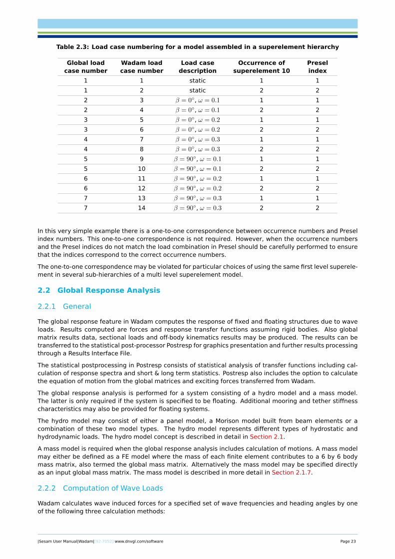
Table 2.3: Load case numbering for a model assembled in a superelement hierarchy
Global loadcase number
Wadam loadcase number
Load casedescription
Occurrence ofsuperelement 10
Preselindex
1 1 static 1 1
1 2 static 2 2
2 3 β = 0◦, ω = 0.1 1 1
2 4 β = 0◦, ω = 0.1 2 2
3 5 β = 0◦, ω = 0.2 1 1
3 6 β = 0◦, ω = 0.2 2 2
4 7 β = 0◦, ω = 0.3 1 1
4 8 β = 0◦, ω = 0.3 2 2
5 9 β = 90◦, ω = 0.1 1 1
5 10 β = 90◦, ω = 0.1 2 2
6 11 β = 90◦, ω = 0.2 1 1
6 12 β = 90◦, ω = 0.2 2 2
7 13 β = 90◦, ω = 0.3 1 1
7 14 β = 90◦, ω = 0.3 2 2
In this very simple example there is a one-to-one correspondence between occurrence numbers and Preselindex numbers. This one-to-one correspondence is not required. However, when the occurrence numbersand the Presel indices do not match the load combination in Presel should be carefully performed to ensurethat the indices correspond to the correct occurrence numbers.
The one-to-one correspondence may be violated for particular choices of using the same first level superele-ment in several sub-hierarchies of a multi level superelement model.
2.2 Global Response Analysis
2.2.1 General
The global response feature in Wadam computes the response of fixed and floating structures due to waveloads. Results computed are forces and response transfer functions assuming rigid bodies. Also globalmatrix results data, sectional loads and off-body kinematics results may be produced. The results can betransferred to the statistical post-processor Postresp for graphics presentation and further results processingthrough a Results Interface File.
The statistical postprocessing in Postresp consists of statistical analysis of transfer functions including cal-culation of response spectra and short & long term statistics. Postresp also includes the option to calculatethe equation of motion from the global matrices and exciting forces transferred from Wadam.
The global response analysis is performed for a system consisting of a hydro model and a mass model.The latter is only required if the system is specified to be floating. Additional mooring and tether stiffnesscharacteristics may also be provided for floating systems.
The hydro model may consist of either a panel model, a Morison model built from beam elements or acombination of these two model types. The hydro model represents different types of hydrostatic andhydrodynamic loads. The hydro model concept is described in detail in Section 2.1.
A mass model is required when the global response analysis includes calculation of motions. A mass modelmay either be defined as a FE model where the mass of each finite element contributes to a 6 by 6 bodymass matrix, also termed the global mass matrix. Alternatively the mass model may be specified directlyas an input global mass matrix. The mass model is described in more detail in Section 2.1.7.
2.2.2 Computation of Wave Loads
Wadam calculates wave induced forces for a specified set of wave frequencies and heading angles by oneof the following three calculation methods:
|Sesam User Manual|Wadam|[92-7052] www.dnvgl.com/software Page 23

• Morison’s equation applied to a Morison model
• The MacCamy-Fuchs formula applied to a Morison model
• The potential theory applied to a panel model
• A method in which Morison’s equation and the potential theory both are applied to compute hydro-dynamic loads on the same hydro model. This type of hydro model is termed a composite modeland is described in Section 2.1.4. With the composite model the wave kinematics applied in Mori-son’s equation may optionally be modified to take into account the diffracted wave field due to thepresence of a panel part in the hydro model.
The motion responses for a hydro model is obtained by solving the equations of motion for a set of wavefrequencies and heading angles. The rigid body added mass, damping and restoring matrices used in theequations of motion may be calculated by applying Morison’s equation, the potential theory or the compositemethod as described above. Except for frequency dependent added mass matrices these matrices mayalternatively be specified directly by the user.
2.2.3 The Global Response Results
The wave induced forces and moments and the motion responses calculated by Wadam are reported withrespect to a motion reference point which is, by default, located at the intersection between the still waterlevel and a vertical line through the common origin of the models used in the analysis. The coordinatesystems in Wadam are described in Section 2.1.1.
The results available from a global response analysis of a hydro model include transfer functions for:
• Wave exciting forces and moments
• Motion responses
• Sectional loads
• Rigid body matrices
• Off-body kinematics
• Surface elevations
Section 2.5 describes all these result types in more detail.
2.3 The Calculation of Detailed Loads on a Structural Model
2.3.1 General
The detailed load calculation feature provides a tool for automatically transferring wave loads from a hydro-dynamic analysis into finite element loads for a structural analysis.
Both hydrostatic and hydrodynamic loads on a structural model may be calculated. The results, which maybe both FE pressure loads and nodal loads, will be transferred to Loads Interface Files for subsequent linearstatic or dynamic analysis in Sestra. Wadam also transfers environmental information and load case num-bering information to Sestra on a separate file (the S-file). The latter is specifically required for a subsequentstochastic fatigue analysis using Framework or Stofat.
2.3.2 The Structural Load Types
Three different load types may be generated by Wadam and transferred to a structural model. Theseare:
• Hydrostatic loads with contributions from forces in the still water condition and pre-tension frommooring and tether systems
• Gravity load representing the weight of the structure
• Hydrodynamic loads with contributions from exciting forces from incident waves, forces from waveinduced motion and rigid body accelerations
|Sesam User Manual|Wadam|[92-7052] www.dnvgl.com/software Page 24

Detailed descriptions of distributed loads are included in Section 2.5.15 and Section 2.5.16.
Wadam generates separate load case numbers for the hydrostatic load and for each of the hydrodynamicloads, i.e. for each wave frequency and heading. When having a superelement hierarchy model, theseloads may be combined into new load cases with Presel. The new combined load cases will be used duringsubsequent structural analysis and postprocessing. Section 2.1.10 contains a more detailed description ofload case numbering and load case combinations in Sesam.
2.3.3 Deterministic Loads
Wadam also provides the option to report transfer functions for FE loads as deterministic loads (time do-main). That is loads represented for specified phase angles of incident waves with given wave ampli-tudes.
The deterministic results presentation may also be used together with the option to calculate the followingtypes of loads:
• Non-linear viscous drag forces from Morison’s equation for fixed structures.
• Pressure loads up to the instantaneous free surface, see Section 2.6.9.
• Time invariant current profiles added to the incident wave field in the calculation of forces by Mori-son’s equation. See Section 2.4.2 for the description of current profiles in Wadam.
2.3.4 Detailed Loads Transfer to a Model with Shell or Solid Elements
The transfer of detailed loads to a large volume structure modelled with shell or solid elements is performedas follows:
• The hydrostatic load at still water condition is calculated as normal pressures directly on the shelland solid element surfaces defined as wet sides.
• The hydrodynamic pressure loads on shell or solid elements can only be obtained from a potentialtheory calculation based on a panel model. The actual mapping of panel pressures into normalpressure loads in a structural model is automatically performed by the algorithm described in Ap-pendix A 3.3.
• Independent nodal loads require a Morison model to be used together with the panel model. Morespecifically, if loads from mooring lines and tethers shall be included in a structural system a Morisonmodel consisting of the connection nodes must be created.
2.3.5 Detailed Loads Transfer to a Model with Beam Elements
The transfer of loads to a slender structure, for example a jacket or a jackup, modelled with beam elementsis performed as follows:
• The hydrostatic load at the still water condition is represented as loads on beam elements and nodesin the structural model.
• The hydrodynamic loads are calculated for the beam elements and nodes corresponding to the Mori-son elements. The hydrodynamic pressure loads obtained by Morison’s equation are representeddirectly as line loads and nodal loads on the beam element model to be transfered to structuralanalysis.
2.4 Environmental Description
2.4.1 Surface Waves
The models in Wadam may when first order potential theory and Morison’s equation are applied be exposedto planar and linear harmonic waves, i.e. waves described by the Airy wave theory. For the second orderoption for the potential theory see [3] for a detailed description of the theoretical background.
|Sesam User Manual|Wadam|[92-7052] www.dnvgl.com/software Page 25

Figure 2.22: Surface wave definitions
The incident waves may be specified by either wave lengths, wave angular frequencies or wave periods. Thedirection of the incident waves are specified by the angle β between the positive x-axis and the propagatingdirection as shown in Figure 2.22 (a).
The incident wave used in Wadam is defined as
η = Re[A ei(ωt−k(x cos β+y sin β))
](2.2)
which alternatively may be written as
η = A cos (ωt− k (x cosβ + y sinβ)) (2.3)
This represents a wave with its crest at the origin for t = 0 as shown in Figure 2.22 (b).
The fluid velocity v = vxi+ vyj+ vzk and acceleration a = axi+ ayj+ azk for the incident waves are:
vh = vxi + vyj = Aωk
k
cosh (kz + kd)
sinh (kd)cos (ωt− k · x)
vz = −Aω sinh (kz − kd)
sinh (kd)sin (ωt− k · x)
(2.4)
ah = −axi + ayj = Aω2k
k
cosh (kz + kd)
sinh (kd)sin (ωt− k · x) (2.5)
az = −Aω2 sinh (kz − kd)
sinh (kd)cos (ωt− k · x) (2.6)
where
d Depth
k Absolute value of wave number
ω Wave angular frequency
A Wave amplitude
x = xi + yj – location in the x-y plane
k = k (i cosβ + j sinβ) – two dimensional wave number
z Vertical coordinate with z-axis upward, z = 0.0 at still water level
β Direction of wave propagation
The finite depth dispersion relation used in the above expressions is
ω2 = gk tanh (kd) (2.7)
The wave period is given by
T =2π
ω(2.8)
|Sesam User Manual|Wadam|[92-7052] www.dnvgl.com/software Page 26

and the wave length is
λ =2π
k(2.9)
For a more detailed description of linear wave theory see [8].
The fluid kinematics above the still water level is obtained by constant extrapolation in Wadam.
2.4.2 Current Profiles
Wadam provides the option to specify time invariant current profiles for the calculation of deterministicMorison element forces.
Note: The current profile can only be used for fixed structures.
The current profile may be specified at a set of positions along the z-axis of the global coordinate system.Current values at intermediate z-positions are obtained by linear interpolation. The direction of the currentin the horizontal plane is specified at each positions.
Figure 2.23: Current profile definition
2.4.3 Water Depth
Wadam provides the option to specify a water depth. The water depth is used in two different calculationphases in the program:
• It is used in the processing of the panel model to remove all panels below the sea-bed.
• It is used in the calculation of Green’s functions for finite water depth.
2.5 Results Types Reported from Wadam
2.5.1 Units
When performing an analysis with Sesam the user must apply a set of consistent units. The same units mustbe used in all programs throughout the analysis from modelling to results presentation.
The basis for determining a set of consistent units is the fundamental equation:
f = ma (2.10)
In terms of the fundamental units of mass [M], length [L] and time [T] this equation may be written:[F =
ML
T2
](2.11)
|Sesam User Manual|Wadam|[92-7052] www.dnvgl.com/software Page 27

Force, stress, density, etc. are not fundamental units and must be derived in terms of the units of mass,length and time. Whenever possible it is simplest to use S.I. units:
[L] Length in meters (m)
[M] Mass in kilograms (kg)
[T] Time in seconds (s)
Force will then be in Newton (N):
1N = 1kg m
s2(2.12)
The units used in Wadam is controlled by the acceleration of gravity [L/T2] and the fluid density [M/L3]. Allother input data must be expressed in terms of these units. For example:
• Fluid kinematic viscosity: [L2/T]
• Fluid velocity: [L/T]
2.5.2 Result Reference Point
For single-body structures the results from Wadam are reported with respect to a default result referencepoint which is coinciding with the origin of the global coordinate system; see Section 2.1.1. For multi-bodystructures there is one result reference point for each body coinciding with the body coordinate systems;see Section 2.1.6.
The result reference point can also be specified by the user. In this case, the user specifies the displacementof the result reference point relative to the default point. The displacement is given for all three directions ofthe axes of the global coordinate-system. The results relative to the user-specified result point are obtainedby linear transformations of the end-results. The drift-forces are then not transformed correctly to secondorder in the amplitude and should normally not be used in this context.
2.5.3 Dimensioning of Results
Wadam reports results on dimensionalised and non-dimensionalised form as follows:
• The Hydrodynamic Results Interface File contains dimensionalised results.
• The Loads Interface Files contain dimensionalised results.
• The Wadam print file contains both forms as follows:
– Chapters 2 and 5 contain dimensionalised results.
– Chapter 4 contains non-dimensionalised results.
Table 2.4: Dimensionalising factors for matrices
Dn entryi,j
Result type i = 1-3, j = 1-3i = 1-3, j = 4-6i = 4-6, j = 1-3 i = 4-6, j = 4-6
Inertia matrix ρV ρV L ρV L2
Added mass matrix ρV ρV L ρV L2
Damping matrix ρV√g/L ρV
√gL ρV L
√gL
Restoring matrix ρV g/L ρV g ρV gL
|Sesam User Manual|Wadam|[92-7052] www.dnvgl.com/software Page 28

Table 2.5: Dimensionalising factors for results
Dn modeiResult type i = 1− 3 j = 4− 6
Exciting forces ρV gA/L ρV gA
Motion A A/L
Drift forces ρgLA2 ρgL2A2
Sectional loads ρV gA/L ρV GA
Fluid pressures ρgA
Fluid velocities√g/LA
Fluid accelerations gA/L
2nd order forces ρgLA2 ρgL2A2
2nd order motions A2/L A2/L2
2nd order pressures ρgA2/L
The non-dimensionalising factor Dn specified in Table 2.4 and Table 2.5 may be used to obtain dimension-alised results Fd from the formula:
Fd = DnFn (2.13)
where Fn is a non-dimensionalised result reported in chapter 4 in the Wadam print file. The factors used inthe tables are:
ρ Density of the fluid
g Acceleration of gravity
L Characteristic length
V Displaced volume of the body
A Amplitude of the incoming wave, equal to one for harmonic results
2.5.4 Transfer Functions and Phase Definitions
The transfer functions in Wadam describe responses for bodies in harmonic waves. The reported responsesare normalised with respect to the incident wave amplitudes. With a transfer function H(ω, β) the corre-sponding time dependent response variable R(ω, β, t) can be expressed as
R(ω, β, t) = ARe[H((ω, β)) eiωt
](2.14)
where A is the amplitude of the incoming wave, ω is the frequency of the incoming wave, β describes thedirection of the incoming wave and t denotes time. The phase angle φ between the incident wave and thetime varying response is defined from
R(ω, β, t) = ARe[|H((ω, β))| ei(ωt+φ)
](2.15)
where |H| is the amplitude of the transfer function. The transfer function and the phase angle may beexpressed as
H = HRe + iHIm and φ = atanHIm
HRe(2.16)
The time varying response can alternatively be expressed as
R(ω, β, t) = A [HRe cosωt−HIm sinωt] (2.17)
The phase lead φ of the response relative to an incident wave with the wave crest at the origin of the globalcoordinate system is shown in Figure 2.24.
|Sesam User Manual|Wadam|[92-7052] www.dnvgl.com/software Page 29

Figure 2.24: Definition of phase between the response and the incident wave
2.5.5 Hydrostatic Results
Wadam calculates the hydrostatic restoring results from the hydro model. It is given with dimensions andinclude:
• The sum of displaced volume of the panel and Morison part of the model
The total displaced volume is reported together with the separate contributions from the panel andMorison parts.
For the panel model the volume is reported from three different calculations, i.e. from summingup of control volumes in the three different directions. The reported total volume is taken as themedian of the three volumes (not mean but middle value of three values).
Note: If the separate control volumes are differing by a significant number this normally indi-cates that the wet surface of the model is not properly defined.
• The centre of buoyancy
• The water plane area
• The metacentric height
• The global hydrostatic restoring matrix assembled from both hull restoring and additional stiffnessterms
The additional hydrostatic stiffness terms included in the hydro model may include contributions from:
• Risers, mooring lines or tethers represented with Morison mooring or tether elements
• Stiffness matrices specified directly on the analysis control data
For multi-body models the hydrostatic restoring matrix for each body is reported.
Note: In the hydrostatic restoring contribution from the Morison elements the local waterplanemoment for each Morison member is not included. This can cause errors if some ofthe beams have a large diameter. The fix to this problem is to include this restoringcontribution as an additional restoring matrix.
2.5.6 Global Mass Matrix
A 6 by 6 mass inertia coefficient matrix is reported for each body. It is generated according to the inputdefinition and hence may be calculated from either:
• The hydro model
• The structural model
• A specific mass model
|Sesam User Manual|Wadam|[92-7052] www.dnvgl.com/software Page 30
• The input definition of an inertia mass matrix based on:
– Specifying the centre of gravity and the radii of gyration together with the total mass
– Specifying the 6 by 6 global mass matrix
2.5.7 Added Mass Matrix
The 6 by 6 added mass matrix is reported for each separate body. The added mass interaction matricesbetween any two bodies in a multi-body system are also reported. The added mass matrix is calculatedaccording to the type of the hydro model as follows:
• Frequency dependent added mass from potential theory
• Frequency independent added mass from Morison’s equation
For the composite hydro model the added mass at a given frequency is reported with both frequency de-pendent and independent contributions.
2.5.8 Damping Matrix
The 6 by 6 damping matrix is reported for each separate body. The potential damping interaction matri-ces between any two bodies in a multi-body system are also reported. The damping matrix is calculatedaccording to the type of the hydro model as follows:
• Frequency dependent damping from potential theory
• Frequency independent linearised viscous damping from Morison’s equation
• HydroD specified frequency dependent or frequency independent 6 by 6 damping matrices
For the composite hydro model type the damping for a given frequency is reported as both frequency de-pendent and independent contributions.
2.5.9 Exciting Forces and Moments
The transfer functions for exciting forces and moments due to the incident waves are reported for each bodyat all the combinations of frequencies and wave headings. The transfer functions for rigid body forces andmoments are calculated as follows:
• By integration of exciting forces from all types of Morison elements obtained from the linearisedMorison’s equation
• By integration of pressures on all the panels obtained by solving the diffraction problem
• By applying the Haskind relation on the radiation potentials if no detailed panel pressures shall becalculated
For the composite model type the exciting forces from the panel and Morison parts are reported both sepa-rately and as the combination used in the subsequent analysis, e.g. in the equation of motion.
By selecting time domain output the above results will be reported as deterministic forces and moments atspecified phases of the incident waves with given wave amplitudes.
For fixed structures the deterministic Morison option may be used to include the following non-linear effectsin Morison’s equation:
• Non-linear viscous drag formulation
• Time invariant current may be superimposed on the fluid velocities.
• Forces and moments may be calculated up to the free surface by constant extrapolation of the linearwave profile.
|Sesam User Manual|Wadam|[92-7052] www.dnvgl.com/software Page 31

2.5.10 Rigid Body Motion
The transfer functions for rigid body motion due to the incident waves are reported for each body for allthe combinations of wave frequencies and heading angles. The roll, pitch and yaw motions are reported inradians.
The equation of motion is assembled from the calculated global matrices and transfer functions as describedin the previous sections. The HydroD specified damping and stiffness matrices will be added to the otherwisecalculated matrices.
By specifying the time domain output format the motions will be reported as deterministic motions at spec-ified phases of the incident waves with given wave amplitudes.
2.5.11 Second Order Mean Drift Forces
The second order mean drift forces due to the linear incident waves are reported both on the print file andin the Hydrodynamic Results Interface File. They are calculated by one of the following methods:
• Momentum conservation in the three horizontal degrees of freedom
• Pressure integration in all six degrees of freedom. This method will also give the mean drift forceson each individual body in a multi-body analysis.
2.5.12 Second Order Sum and Difference Frequency Results
The transfer functions for sum and difference frequencies are reported in the print file and on the Hydrody-namic Results Interface File. The following second order results are available:
• The quadratic second order force
• The second order forces on the body by an indirect calculation method
• The second order pressure distribution on the body (available in the print file and in the Wamitoutput file format)
• The second order wave elevation at specified points (only available in the Wamit output file format)
2.5.13 Fluid Kinematics
The transfer functions for pressure and particle velocity in specified points in the fluid is reported both onthe print file and in the Hydrodynamic Results Interface File. The fluid kinematics points are specified in thefluid domain outside the hydro model. The fluid kinematics depends on the type of hydro model:
• It is obtained from the incident undisturbed wave field if only Morison’s equation is applied.
• It is obtained from the diffracted wave field if the potential theory is applied to a fixed structure.
• It is obtained from the radiated and diffracted wave field if the potential theory is applied to a floatingstructure.
By specifying the time domain output format the fluid kinematics will be reported as deterministic pressureand velocities at specified phases of the incident waves with given wave amplitudes.
The surface elevation η in a radiated and diffracted wave field is obtained from potential theory as
η =p
ρg(2.18)
where p is the non-dimensionalised pressure at the still water level.
2.5.14 Wave Drift Damping
The Wave Drift Damping describes the rate of change of the Mean Drift force with forward speed computedat zero speed. The sign of this rate of change is in most cases negative, meaning that this will representa damping mechanism for the slow drift motion excited by the second-order difference frequency forces ordue to the interaction of the waves with a current.
|Sesam User Manual|Wadam|[92-7052] www.dnvgl.com/software Page 32

The 3x3 Wave Drift Damping matrix (surge, sway, yaw) is reported in the Hydrodynamic Results InterfaceFile. This matrix is computed according to the methods described in [9].
The computation of the wave drift damping requires a free surface mesh which is defined as input exactly likethe free surface mesh for second-order analysis. The mesh used in the Wave Drift Damping computationsdoes, however, not need to have a circular outer boundary.
A Morison model can not be used if Wave Drift Damping is to be computed.
The iterative equation-solver for the potential-solution can not be applied if Wave Drift Damping is com-puted.
2.5.15 Distributed Hydrostatic Loads
The hydrostatic loads on a structural model is calculated directly on the individual finite elements of themodel. It is represented on the Loads Interface Files as a real load case.
Structural Beam Models
For wet beam structural superelements the hydrostatic load case is represented as line loads on the beamfinite elements and as nodal loads on nodes receiving loads from 3D Morison elements and pressure areaelements. In addition, the pre-tension from Morison anchor and TLP elements are included as nodal loads inthe hydrostatic load case.
A general description of line loads on beam finite elements is included in Appendix A 3.2.
Note: Pressure Area Elements should always be defined at the end of vertical members suchas the legs on a semi-submersible.
Structural Shell or Solid Models
For wet surfaces of shell and solid elements in a structural model the hydrostatic loads are representedas normal pressures. Because the hydrostatic pressure intensities are evaluated individually at the z-coordinate of each node the normal pressure on wet element sides will have a variation in the z-direction asopposed to the hydrodynamic loads which are constant over each element.
The gravity component of the static load is included by writing the acceleration of gravity to the LoadsInterface File.
2.5.16 Distributed Hydrodynamic Loads
The distributed hydrodynamic loads are calculated in a body fixed coordinate system and include the follow-ing contributions:
• Exciting forces from incident waves
• Forces from wave induced motion
• Fluctuating hydrostatic pressure forces due to the body motion
The distributed forces presented in the Wadam print file are:
• Transfer functions for pressures on the panels in the hydro model 1
• Transfer functions for forces acting at the centre of gravity for 2D Morison elements
• Transfer functions for nodal forces acting on nodes in the hydro model which are connected to thefollowing Morison element types:
– 3D Morison elements
– Pressure area elements
– Mooring and TLP elements
The distributed loads transferred to the Loads Interface Files are:1Not including fluctuating hydrostatic pressure.
|Sesam User Manual|Wadam|[92-7052] www.dnvgl.com/software Page 33

• Transfer functions for normal pressures on the wet sides of shell and solid elements. The pressuresare constant over the elements. These loads originate from pressures at the centroid of panels ac-cording to the mapping algorithm described in Appendix A 3.3. They include fluctuating hydrostaticpressure.
• Transfer functions for line loads on beam elements. These loads originate from forces at the centreof gravity of 2D Morison sub-elements and dry Morison elements. The calculation of line loads on 2node beam elements is described in Appendix A 3.2.
• Transfer functions for loads at nodes which are connected to Morison elements
• An acceleration field acting on all the nodes in the structural model
• The inertia components are only included as loads if the mass model is specified as a distributedmass model.
Wadam and the structural analysis program Sestra both employ the standard Sesam finite element libraryto generate a mass representation. This implies that the connection between accelerations and inertia loadsis consistently handled in the two programs.
2.5.17 Load Sum Reports
Load sums are important tools to verify both the correctness of input models to Wadam and of the consis-tency between Wadam and subsequent structural analyses.
Wadam reports load sums on both the structural model and the hydro model in chapter 5.1 in the print file.Note that these load sums are reported with dimensions.
• Load sums for the loads transferred to the structural beam model:
– The sum of hydrostatic loads transferred to a beam model is reported in the print file asstatic loads. It includes the hydrostatic forces from each Morison type of element as follows:
∗ The buoyancy and pre-tension components from mooring and TLP elements are al-ways included.
∗ The gravity components are only included if the mass model is specified as a dis-tributed mass model.
– The sum of hydrodynamic loads acting on the beam model is reported in the print file foreach incident wave frequency and wave heading. It includes the hydrodynamic forces fromeach Morison type of element as follows:
∗ The hydrodynamic pressure components acting on beams and nodes
∗ The inertia components are only included if the mass model is specified as a dis-tributed mass model.
• Load sums for the loads transferred to the structural shell/solid model:
– The sum of hydrodynamic pressure loads transferred to the shell and solid structural modelis reported in the print file for each incident wave frequency and wave heading. It includesthe part of the hydrodynamic loads actually transferred to normal pressure loads on shelland solid elements. Note that this load sum does not include inertia loads.
– The sum of pressures and inertia loads acting on the structural model may be calculatedfrom the Sestra data check where the accelerations transferred from Wadam are convertedinto inertia loads; see Section 2.5.16.
• Load sums for the hydro model:
– The sum of hydrodynamic forces acting on a panel model is reported in the print file foreach incident wave frequency and heading. It includes the pressures acting at the centroidof each panel in the hydro model. Note that this load sum does not include inertia loads.
|Sesam User Manual|Wadam|[92-7052] www.dnvgl.com/software Page 34

2.5.18 Sectional Loads
Wadam calculates sectional loads by integration of distributed forces on specified sides of given planes inter-secting a hydro model. The frequency dependent exciting and inertia forces are included in the integration.The sectional planes are specified in the input coordinate system and must be normal to one of the mainaxes of the global coordinate system. A moment reference point is specified for each plane. Figure 2.25displays a simple submerged beam model with a sectional plane xinp = 0. The moment reference point isdefined in the input coordinate system (xinp, yinp, zinp).
Figure 2.25: Sectional loads at a plane through x = 0
The sectional loads are reported in the Wadam print file and on the Hydrodynamic Results Interface File ascomplex transfer functions.
Still water sectional loads are reported on the Wadam print file.
The sectional loads are integrated with respect to a body fixed coordinate system. The sectional load on acut comes from the integration of F-ma over that part of the structure which is on the positive or negativeside of the cut. The components of the load are in the global system. This means that for the dynamicloads the load computed by integration over the positive side and the load computed by integration overthe negative side will be equal in magnitude, but have a phase difference of 180 degrees.
As an example we consider a ship cut at x = 0 normal to the x-axis:
If integration over the positive side is specified the sectional load will be the force acting on the part of thehull with x < 0 from the part with x > 0. This means that the static bouyancy force will give a positivevertical shear force and a negative vertical bending moment. We will also find that the phase angle of thevertical bending moment in a hogging situation is close to zero for long waves.
If integration over the negative side is specified the static bouyance force will give a positive vertical shearforce and a positive vertical bending moment. The phase angle for the vertical bending moment in a longwave will be close to +/- 180 degrees.
The contributions to the sectional loads from different hydro models are computed as follows:
• For Morison models the exciting and inertia forces, obtained at the centre of gravity of each Morisonsub-element on the specified side of the sectional plane, are included.
• For panel models the exciting forces at the centroid of each panel are included. The inertia forcesare included with respect to a centre of gravity calculated for the part of the model that is on thespecified side of the sectional plane.
• For panel models the sectional loads from integrating the hydrostatic pressure loads on the panelmodel are also reported in the print file (LIS-file).
Note: Sectional loads calculation should be used with care when global matrices are specifieddirectly as input to Wadam. This is because the global matrices do not provide thedetailed information required to integrate distributed force contributions.
In addition to the total sectional loads it is also possible to compute and write to the Global Results InterfaceFile (G-file) differnt parts of the sectional load. This includes sectional added mass matrix, sectional dampingmatrix, sectional body mass matrix and sectional excitation force. These quantities cannot be handled byPostresp, but they may be read into DeepC.
|Sesam User Manual|Wadam|[92-7052] www.dnvgl.com/software Page 35

To compute these sectional load details a modification of the Wadam*.FEM file must be done manually: Openthis file in an editor an find the card WADAMA1. (This is one of the first cards on the file.) Change the 19thnumber on this card from 0 to 1.
2.5.19 Roll Damping Coefficients
Wadam calculates the roll damping coefficient B44 by including contributions from the following hydrody-namic effects:
• Potential damping from surface wave radiation
• Linearised viscous damping from skin-friction of the hull
• Linearised viscous damping from eddy-making
• Linearised viscous damping from bilge keel
The potential damping effect is included in the radiation potentials and is defined within the regular lineartheory.
The linearized viscous roll damping effects from eddy-making due to the naked hull is computed based onempirical data given by Tanaka, [6], while the damping coefficient from skin-friction and eddy-making frombilge keels are computed according to Kato, [7]. These originally non-linear viscous damping contributionsare linearised in order to be included in the harmonic equations of motion.
The potential damping and the skin friction contributions are calculated from a strip model which is auto-matically generated from a panel model. The other two effects are calculated from information about thebilge keel.
From version 9.3 of Wadam, a new roll damping model is available which is based on ITTC RecommendedProcedures [14]. The new model is different from Tanaka/Kato’s approach in the method on evaluating theeddy-making and bilge keel damping components. In addition, a simplified formula is implemented for pre-dicting the eddy-making component of a sharp-corner box hull with very shallow draught. Moreover, The hulllift damping component will be added when the forward speed is given for roll damping calculation.
The viscous damping coefficient is generally defined as
B∗44 = Kη4max
In Wadam the coefficient K is calculated approximately as a function of the wave-frequency, the hull formand the bilge keel dimensions. The variable η4max is the maximum expected roll angle.
When viscous roll damping is included in the equation of motion the roll angle amplitude is not known inadvance rather it is a part of the solution. Therefore, the user has to estimate the maximum expected rollangle for each wave heading. The calculated transfer function for roll motion is compared with the maximumvalue specified for that heading. If the computed roll motion is ’close’ to the specified angle then the rolltransfer function for that value is assumed to be ’correct’. If the difference is not acceptable then anotherη estimate must be made and the roll motion re-computed. Note, however, that the potential solution isindependent of η. Hence the potential should be saved during the first computation and the program shouldbe submitted with a restart option during this iteration process. If the maximum roll angle is taken fromshort term statistics (only one sea state) then Wadam can perform the iteration process automatically. If themaximum roll angle is taken from long term statistics then the iteration must be carried out manually.
It should be kept in mind that these coefficients are only valid within the range of tests and models used inthe experiments. Extrapolation outside this range should be performed with care.
The roll damping option in Wadam also includes a linearised roll restoring coefficient in the equation ofmotion. The calculation of this coefficient is described in Appendix A 3.1.
Note: The Roll damping model can only be used for ship-like structures with symmetry aboutthe XZ-plane.
Note: When Tanaka/Kato approach is applied, the computation of the bilge keel dampingbreaks down when the bilge keel is very small. The symptom is that the damping startsto increase when the width of the bilge keel decrease. The exact limit is case dependent,but as an indication the width of the bilge keel should not be smaller than 10 cm.
|Sesam User Manual|Wadam|[92-7052] www.dnvgl.com/software Page 36

2.5.20 Global drag-coefficient for roll-damping
A global coefficient for quadratic damping of the roll-motion can be given as user-specified input. Thismakes it possible to use results from model-tests directly. The quadratic damping is linearized by stochasticlinearization. This way, model tests performed independent of sea-states can be used in connection withany given sea-state valid for the actual location of the structure. The formulation of the method of stochasticlinearization is explained in Appendix A 3.5.
Note: This kind of damping should not be combined with any other types of damping effects,except the potential dampimg. In other words, the old roll-damping model, the Morisonmodel or user-specified linear damping are not to be combined with the global tortionaldrag.
2.6 Calculation Methods
2.6.1 Calculation of Wave Loads from Potential Theory
The potential theory as described in Newman, ref. [1], is applied in Wadam to calculate first order radiationand diffraction effects on large volume structures. The actual implementation is based on Wamit2, ref. [2],which uses a 3D panel method to evaluate velocity potentials and hydrodynamic coefficients.
This implementation can be used for infinite and finite water depths and both single bodies and multipleinteracting bodies can be analysed. The flow is assumed to be ideal and time-harmonic. The free surfacecondition is linearised for the first order potential theory while the non-linear free surface condition is im-posed for the second order potential theory computation. The radiation and diffraction velocity potentials onthe wet part of the body surface are determined from the solution of an integral equation obtained by usingGreen’s theorem with the free surface source potentials as the Green’s functions. The source strengths areevaluated based on the source distribution method using the same source potentials.
The integral equation is discretisized into a set of algebraic equations by approximating the body surfacewith a number of plane quadrilateral panels. The source strengths are assumed to be constant over eachpanel. Two, one or no planes of symmetry of the body geometry may be present. The solution of thealgebraic equation system provides the strength of the sources on the panels. The equation system, which iscomplex and indefinite, may be solved by a direct LU factorization method or by an iterative method.
When using the direct solver, the integral equation is solved directly for each frequency. The time spentfor different wave frequency is virtually equal. In comparison, more iterations are needed for shorter wavesthan for long waves when running with iterative solver. In addition, some more effort is required for differentwave headings comparing with the direct solver. Moreover, iterative solver is more sensible to the meshquality. Generally, the CPU time for direct solver is increasing with panel number following O(N)
3 whereasiterative solver is following O(N)
2, where N is the total panel number in an analysis. It is suggested thatdirect solver shall be used when N is less than 10000 and with many wave headings included. Whereas theiterative solver becomes more favorable when N is more than 15000.
Boundary Value Problem Formulation
The assumption of potential flow allows defining the velocity flow as the gradient of the velocity potential Φthat satisfies the Laplace equation
∇2Φ = 0 (2.19)
in the fluid domain. The harmonic time dependence allows defining a complex velocity potential φ relatedto Φ by
Φ = Re(φ eiωt
)(2.20)
where ω is the frequency of the incident wave and t is time. The associated boundary-value problem willbe expressed in terms of the complex velocity potential φ with the understanding that the product of allcomplex quantities with the factor eiωt applies. The linearised form of the free-surface condition is
φz −Kφ = 0, on z = 0 (2.21)
2Wamit is a computer program developed by Massachusetts Institute of Technology.
|Sesam User Manual|Wadam|[92-7052] www.dnvgl.com/software Page 37

where K = ω2/g and g is the acceleration of gravity. The velocity potential of the incident wave is definedby
φ0 =igA
ω
cosh (kz +H)
cosh kHe−k(x cos β+y sin β) (2.22)
where the wave number k is the real root of the dispersion relation and β is the angle between the directionof propagation of the incident wave and the positive x-axis.
Linearisation of the problem permits decomposition of the velocity potential φ into the radiation and diffrac-tion components:
φ = φR + φD, φR = iω
6∑j=1
ξjφj , φD = φ0 + φ7 (2.23)
The constants ξj denote the complex amplitudes of the body oscillatory motion in its six rigid-body degreesof freedom and φj the corresponding unit-amplitude radiation potentials. The velocity potential φ7 repre-sents the disturbance of the incident wave by the body fixed at its undisturbed position. The total diffractionpotential φD denotes the sum of φ7 and the incident wave potential.
On the undisturbed position of the body boundary the radiation and diffraction potentials are subject to theconditions
φjn = nj , φDn = 0 (2.24)
where (n1, n2, n3) = n and (n4, n5, n6) = r × n, where r = (x, y, z). The unit vector n is normal to the bodyboundary and points out of the fluid domain. The boundary value problem must be supplemented by acondition of outgoing waves applied to the velocity potentials φj , for j = 1, ..., 7.
The boundary value problems Equation (2.19) - Equation (2.24) are solved by using Green’s theorem toderive integral equations for the radiation and diffraction velocity potentials on the body boundary. Theintegral equation satisfied by the radiation velocity potentials φj on the body boundary takes the form
2πφj(x) +
∫∫Sb
φj(ξ)∂G(ξ;x)
∂nξdξ =
∫∫Sb
njG(ξ;x)dξ (2.25)
where Sb denotes body mean wet surface. The Green function G(ξ;x) represents the velocity potential atthe field point x due to a point source located at point ξ.
The corresponding equation for the total diffraction velocity potential φD is
2πφD(x) +
∫∫Sb
φD(ξ)∂G(ξ;x)
∂nξdξ = 4πφ0(x) (2.26)
When the fluid velocity components are to be calculated, the integral equation take the following generalform for source instead of velocity potential.
2πσ(x) +
∫∫Sb
σ(ξ)∂G(ξ;x)
∂nxdξ =
∂φ(x)
∂nx(2.27)
2.6.2 Calculation of Wave Loads from Second Order Potential Theory
The second order theory applied in Wadam is described in [3] and [4]. Wadam calculates sum- and difference-frequency components of the second order forces, moments and rigid body motions (Quadratic TransferFunctions) in the presence of bi-chromatic and bi-directional waves.
|Sesam User Manual|Wadam|[92-7052] www.dnvgl.com/software Page 38

2.6.3 Removal of Irregular Frequencies
Wadam provides an option to remove the irregular frequencies from the radiation-diffraction solution. Thismethod is based on extending the integral equation Equation (2.25) and Equation (2.26) to include a panelmodel of the interior water plane,(
2π
−4π
)φ(x) +
∫∫Sb+Si
φ(ξ)∂G(ξ;x)
∂nξdξ =
∫∫Sb
∂φ(ξ)
∂nξG(ξ;x)dξ, x ∈
(Sb
Si
)(2.28)
where Si denotes the interior free surface. Equation (2.28) indicates a fixed body (or free surface) conditionon the interior free surface panels. The corresponding equation for the source formulation is taking thefollowing form.(
2π
−4π
)σ(x) +
∫∫Sb+Si
σ(ξ)∂G(ξ;x)
∂nxdξ =
∂φ(x)
∂nx, x ∈
(Sb
Si
)(2.29)
The panel model of the water plane can be automatically created by Wadam or provided by the user (fromversion 9.3). When the automatic meshing option is applied, panels on the interior free surface is appendedto the panel model of each body, and the connectivity between the free surface panels and the waterlinesegments is enforced. However, this option should not be used for the body, if a ray from the centroidof the water-plane area could intersect the waterline more than once, for example, a floater with multiplecolumns or a drilling ship with a moon-pool. Instead, a separated panel model for the interior water-planearea should be provided. Such a panel model can be included as a dummy body in a multi-body analysis.One may check Section 2.1.6 to determine the order of the bodies when this option is used. It should benoted that the connectivity between the free surface panels and those on the wet hull surface on waterlinesegments is recommended but not mandatory.
2.6.4 Damping free surface lid
It is known that linear potential flow theory over-predicts the free surface elevations in a confined water-plane area, for example, the gap between two ship-hulls or the moon-pool area of a drilling ship. Wadam(from version 9.3) provides an option to suppress the unrealistic free surface elevations with an panel modelplaced on the confined water-plane area with a imposed damping free surface condition as following.
φn = Kφ(1− 2iε− ε2), on Se (2.30)
Comparing with Equation (2.21), the additional terms with linear damping factor ε are added on the exteriorfree surface area Se .
The integral equation Equation (2.25) and Equation (2.26) are extended to include a panel model of theexterior water plane where the linear damping is imposed.(
2π
4π
)φ(x)+
∫∫Sb
φ(ξ)∂G(ξ;x)
∂nξdξ+K(2iε+ε2)
∫∫Se
φ(ξ)∂G(ξ;x)
∂nξdξ =
∫∫Sb
∂φ(ξ)
∂nξG(ξ;x)dξ, x ∈
(Sb
Se
)(2.31)
The corresponding equation for the source formulation is taking the following form.(2π
4π
)σ(x) +
∫∫Sb+Se
σ(ξ)∂G(ξ;x)
∂nxdξ =
(∂φ(x)∂nx
Kφ(1− 2iε− ε2)
), x ∈
(Sb
Se
)(2.32)
The panel model for the damping free surface lid can be included as a dummy body in a multi-body analysis.One may check Section 2.1.6 to determine the order of the bodies when this option is used. The lineardamping factor ε is determined by the geometry of the confined water area and can be obtained from modeltest.
|Sesam User Manual|Wadam|[92-7052] www.dnvgl.com/software Page 39

2.6.5 The Equation of Motion
The equation of motion in Wadam is established for harmonic motion of rigid body systems expressed in theglobal coordinate system.
By applying Newtons law and including the added mass, damping and exciting force contributions acting onthe panel and Morison parts of a hydro model the complex 6 by 1 motion vector X(ω, β) can be found fromthe equation of motion[
−ω2 (M + A(ω)) iω (B(ω)p + Bv) + C + Ce
]X(ω, β) = F(ω, β) (2.33)
where
M represents the 6 by 6 body inertia matrix
A(ω) represents the 6 by 6 frequency dependent added mass matrix
B(ω)p represents the 6 by 6 frequency dependent potential damping matrix
Bv represents the 6 by 6 linearised viscous damping matrix
C represents the 6 by 6 hydrostatic restoring matrix
Ce represents the 6 by 6 external restoring matrix
F(ω, β) is the 6 by 1 complex exciting force vector for frequency ω and incident waveheading angle β
The eigenvalues λ and eigenvectors Φ of the rigid body system is obtained for a given incident wave fre-quency by solving the eigenvalue problem
[−λ (M + A(ω)) + C] Φ = 0 (2.34)
The natural periods of the rigid body system at a given incident wave frequency is expressed as
T =2π√λ
(2.35)
2.6.6 Morison’s Equation
Morison’s equation is used in Wadam to calculate contributions to the equation of motion Equation (2.33)and to calculate the detailed forces F acting on 2D Morison elements and 3D Morison elements. The formof Morison’s equation used in this calculation is given in Equation (2.36) with the effect of relative motionincluded.
F = ω2 (M + ρVMCa)− ω2ρVM (Ca + I)x + iωB (x− ξ) + fc + fg + fb (2.36)
|Sesam User Manual|Wadam|[92-7052] www.dnvgl.com/software Page 40

where
ω Incident wave frequency
M 3 by 3 diagonal mass inertia matrix
Ca 3 by 3 diagonal added mass coefficient matrix
I 3 by 3 identity matrix
ρ Density of water
VM Displaced volume of the Morison element
B Linearised viscous damping matrix expressed as B = 12ρσCD · 8
3πVmax
CD 3 by 3 diagonal drag coefficient matrix
σ Projected area of the Morison element
x Complex amplitude of the incident wave field
ξ Complex amplitude of the motion
fc Fluctuating hydrostatic restoring force representing the first order restoring contribu-tions integrated in the equation of motion
fg Fluctuating gravity force representing the acceleration of gravity calculated in a coor-dinate system fixed with the Morison model
fb Fluctuating buoyancy force calculated in a coordinate system fixed with the Morisonmodel
The linearised viscous damping matrix B in Morison’s equation (Equation (2.36)) is obtained from linearisa-tion of the general viscous drag force FD expressed as
FD =1
2ρσCD (v − x) |v − x| = 1
2ρσCD
8
3πVmax (v − x) = B (v − x) (2.37)
The term
8
3πVmax (2.38)
is a standard result obtained by assuming equal work done at resonance by the non-linearised and theequivalent linear damping term. Vmax is a linearising velocity amplitude specified as input to Wadam. Theone and same Vmax is applied in the linearised drag force calculation for all the motion modes and for all theincident wave frequencies.
For deterministic analysis of fixed structures Morison’s equation is expressed on the form
F = ρVM (1 + Ca) v +1
2ρσCDv|v| (2.39)
where time independent current may be included in v.
The contributions from Morison elements are calculated in the particular element local coordinate systems.The contributions are transformed into the body coordinate system prior to the assembling of rigid bodyquantities.
The wave kinematics in Equation (2.36) and Equation (2.39) may be taken from the incident wave field asdescribed in Section 2.4.1. Optionally the wave kinematics may also be taken from the diffracted wave fieldcalculated from potential theory.
2.6.7 Calculation of Tank Pressures, Quasi-static Method
Wadam calculates by an approximate algorithm the harmonic pressure load on the wet finite element sidesin internal tanks.
|Sesam User Manual|Wadam|[92-7052] www.dnvgl.com/software Page 41

The loads are calculated by applying a hydrostatic pressure distribution in the accelerated reference framefixed with respect to the tank. The pressure load is divided in a constant and an oscillating part and repre-sented by separate load cases. The pressure gradient is given by
∇p = ρ (g − a) (2.40)
where g is the acceleration due to gravity, a is the complex acceleration of the mid-point of the tank and ρ isthe mass density of water. The gravity vector described in a coordinate system oscillating with the body hasa constant and an oscillating part. Accordingly, the pressure gradient described in the body-fixed coordinatesystem has a constant part ρg and an oscillating (dynamic) or fluctuating part:
∇pf = ρ (gf − a) (2.41)
where gf is the fluctuating part of gravity. A detailed outlining of the tank pressure calculation is included inAppendix A 3.4.
The tanks are modelled by defining wet surfaces for the tanks, in separate load cases. See also Section 2.1.8.The number of the loadcase will be one higher than the number of the tank. The loadcase numbering muststart at 2, since the wet surfaces with load case 1 are for the external pressure. All surfaces with the sameload case number will be assumed by Wadam to be part of the same tank.
The filling of the tanks is controlled by assigning the hydro-pressure load only to the wet part of the tankwalls. No sloshing effects are included in this formulation and no moments of inertia about the center ofmass of the fluid are accounted for.
By default, the gradient-value is computed in an approximation to the centroid of the tank and the point ofzero pressure is taken as an aproximated centroid of the "roof "of the tank. These reference-points may, insome cases, not be adequate to use. Because of this, the user has the possibility to specify on input, thepreferred coordinates for gradient-point and point of zero for each tank. The coordinates of the points aregiven in the input system of the model. The user may choose, whether only the gradient-point, only thepoint of zero, or both are to be given as input.
Note: The mass of the tank fluid must be included in the mass model for Wadam. In thestructural (FE) model the inertia forces from the tank fluid are represented as pressureloads and should therefore not be included in the structural mass.
2.6.8 Calculation of Tank Pressures, Full Dynamic Method
As an alternative approach to the quasi-static method, the full dynamic method can be selected to solve thepotential flow problem in the isolated fluid domain for each tank (see [10], [11] and [12]) .
The added mass and restoring stiffness of each tank enter into the global motion equation and the radiationpotentials with the resulting motions determine the actual pressure loads in the tanks with the given internalfree surface level:
∇p = −ρ (Φi + gz) (2.42)
in which, Φ is the total radiation potential in a tank.
To calculate the internal tank fluid dynamics, tank definitions shall be included in the panel model, followingthe same practice as for the tanks in the structure model. The geometry, wet surface, and the load casenumbers shall correspond to those in the structure model, so that correct load transfer mapping can besecured.
Tanks are classified into three types: empty, partially filled and fully filled. The empty tanks are bypassed inthe calculation. For a partially filled tank, the zero point of the hydrostatic pressure is, by default in HydroD,put to the mean internal free surface level. The adjustment of the panels at the internal tank surface iscarried out in the same way as for the external wet panels. For a fully filled tank, the zero point of thehydrostatic pressure is, by default in HydroD, at the top point of the tank geometry. It may also, by the user,even be defined above it. A panel element located at the roof center is found by Wadam to have the zerodynamic pressure for a fully filled tank. It should be noted that, different from the quasi-static method, theacceleration reference point (gradient point) is not used.
|Sesam User Manual|Wadam|[92-7052] www.dnvgl.com/software Page 42

Moreover, the tank fluid shall be excluded from the mass model, since it is represented by the added massfrom the internal radiation problem.
Wadam version 9.0.4 assumes the internal tanks take the same symmetry property as for the external wethull. From version 9.1 of Wadam, the symmetry could be different between tanks and external hull. It shouldbe noted, HydroD Version V4.6-03 prepares the input to Wadam in such a way that the symmetry propertyfor all tanks follow the symmetry property for external wet hull. However, With version newer than V4.6-03,HydroD always assumes that there is no symmetry at all for tanks, so that the complete geometry shall begiven for each tank in the panel model.
2.6.9 Pressure Loads up to Free Surface
Wadam may be used to extrapolate to the free surface the panel pressures calculated by first order potentialtheory (up to the still water level). Note that this implies that the dry finite elements below the still waterlevel will receive no loads when the free surface is below the still water level as shown in Figure 2.26.A constant extrapolation, also called stretching, of pressures above the still water level is applied. Thispressure extrapolation option depends on the amplitudes of the waves and hence this option is only availablewhen results in the deterministic output format is specified.
Figure 2.26: Constant extrapolation of panel pressures to the free surface
Note that the pressures only will be received by the finite elements above the still water level defined aswet in the structural model.
For a panel model this option is available for both fixed and floating structures, but the intersection of thestructure and the free surface must be vertical. If a Morison model is included the option is only availablefor fixed structures.
2.6.10 Reduced pressure up to the free surface
One of the "stretching" methods is the approach referred to as reduced loads. This is a kind of "mean-stretching" applied in frequency domain.
In this procedure, the loads are multiplied with a linearly attenuated reduction factor in a zone betweensome given distance below and above the still-water level. Below the still-water level, the reduction factoris applied directly. Above the still-water level, the reduction factor is applied to the loads extrapolated fromjust below (ideally at) the still-water level.
The loads are attenuated linearly down to zero as the level increases from still-water level and up to a givenamplitude. This amplitude is typically an extreme-level of the waves (eg a 20 year level). For an amplitudeA the pressure load on a panel with centroid at level zc above the still-water level zw are then:
PR = wP0; zw ≤ zc ≤ A (2.43)
where P0 is the pressure at the panel-centroid nearest to still-water level approximately vertically below thepanel with centroid at zc and w is the linear attenuation factor defined by
w =A− (zc − zw)
2A(2.44)
The reduction is continued down below the still-water level, but is then applied to the pressure at the panel-centroid:
PR = wP (zc); A ≤ (zc − zw) < 0 (2.45)
|Sesam User Manual|Wadam|[92-7052] www.dnvgl.com/software Page 43

where P (zc) is the pressure at the panel-centroid at zc. P (zc) and P0 are the standard pressure-calculationsfrom the boundary value problem bounded by the still-water level.
The pressure reduction procedure is only applicable to vertical, or nearly vertical, sides of the body, typicallythe mid-section of a ship hull. The limits in x-direction, of the region we want to apply pressure-reduction oncan be given as input. If no limits are given the program tries to perform pressure reduction on the wholebody.
2.6.11 Wave-current interaction
Based on the perturbation expansion used for the wave-drift damping calculation (see [9]), results for theRAO’s for a small current or forward speed, are obtained. Added mass and damping matrix and fluid velocityat off-body points are still presented only for zero speed. This feature can not be combined with dynamictank pressure approach in the same analysis. A comparative study between Wadam and two other computerprograms is presented in [13], where it is indicated that Wadam can be applied to the conditions with currentspeed up to around 1-2 m/s.
2.7 The Save-Restart System
The save-restart option in Wadam provides a mechanism to store potentials from the solution of the ra-diation and diffraction problem from one Wadam run to the next. Hence, for a given model the radiationand diffraction potentials for combinations of incident wave frequencies and heading angles need only becalculated once.
The save-restart file may be viewed as a database for the calculated potentials. That is, potentials fordifferent combinations of frequencies and heading angles may be appended to the save-restart file from asequence of runs. Furthermore, Wadam may extract potentials for a subset of the frequencies and headingangles stored on the file.
If the model is changed the save-restart database (Wadam.RSQ) must be deleted. Otherwise Wadam will notrun. Notice, however, that when Wadam is executed from HydroD this application allows for managementof multiple restart databases.
|Sesam User Manual|Wadam|[92-7052] www.dnvgl.com/software Page 44

3 USER’S GUIDE TO WADAM
This chapter describes how to use Wadam to analyse typical hydrodynamic problems involving fixed, float-ing and tethered structures. Simple tutorial examples as well as more real life engineering problems arepresented. Some practical modelling guidance is also provided.
The examples have been selected to demonstrate the main features of Wadam. They do not cover all optionsin the program. The text for each example explains the options used in that specific example only.
The panel models shown in this section may be used as guidance during the modelling phase. It is howeverimportant to create a panel model suitable for the type of analysis to be performed. A panel model that issuitable for global response analysis is not necessarily acceptable for other types of analyses. This remarkis equally important for the structural model.
3.1 Column-stabilized Unit
A column-stabilized unit can refer to a TLP or a Semi-submersible. The hydrodynamic analysis on a column-stabilized unit normally involves both potential flow theory applied on a panel model and Morison equationsapplied on a Morison model. The following calculations are performed in Wadam for global response analysis.The first two points are automatically calculated while the rest is optional for this analysis.
• Hydrostatic calculation in which both the hydrostatic and inertial properties for the structure arecalculated
• Calculation of hydrodynamic exciting forces, added mass, damping and global motion response
• Eigenvalue calculations for rigid body motions. One set of eigenvalues is calculated for each waveperiod.
• Sectional forces in specified sections. These are used for selection of waves to be used in a structuralanalysis.
• Calculation of constant drift forces and moments including the effect of motion. These are used in asucceeding analysis where the maximum offsets are calculated.
• Calculation of fluid kinematics in specified points used for air gap and wave up welling analyses. Thefluid kinematics include the effect of radiation and reflection of waves from the floater.
In case a structure model is included in the analysis, the following detailed loads will be calculated andtransfered to the structure model.
• Hydrostatic loads
– Gravity acceleration force
– Hydrostatic pressure
– Pretension force acting on anchor/TLP elements
– Buoyancy force on Morison beams and nodes
• Hydrodynamic loads
– Rigid body accelerations and fluctuating gravity
– Hydrodynamic pressure caused by radiation, diffraction and incoming waves
– Restoring pressure induced by the body heave, pitch and roll motions
– Reaction forces on anchor/TLP elements caused by rigid body motions of the floater
– Morison force as line loads on beams where Morison sections are defined
– Fluctuating buoyancy force and incoming wave pressure on nodes when pressure area ele-ments are defined with Morison model
Preparation for this analysis in Wadam consists of the following steps:
• Creation of the panel model in GeniE or Patran-Pre. Symmetry of the structure can be utilized sothat and only one quarter or half of the wet hull is modelled
|Sesam User Manual|Wadam|[92-7052] www.dnvgl.com/software Page 45

• Creation of beam elements for the Morison model in Patran-Pre or GeniE
• Creation of structural model in Patran-Pre or GeniE
• Including the above Input Interface Files in HydroD, define relevant properties, define mass modeland loading condition
• Specifying environmental properties and execution directives where computation parameters andoptions are specified.
Panel Model
The basic part of the panel model for a TLP is shown in Figure 3.1. Since the TLP is double symmetric onlyone quarter of the panel model is modelled. The remaining parts of the model are generated in Wadam bythe symmetry option.
Figure 3.1: Basic part of the TLP panel model from two view points
The basic part of the panel model is modelled as one first level superelement in Patran-Pre or GeniE. It isrequired that it is modelled in quadrant one, that is with x, y ≥ 0. The input coordinate system is located atthe water level in the centre of the TLP.
The wet sides of the panel model are identified in in Patran-Pre or GeniE by dummy hydro pressure actingtowards the wet hull from the fluid.
The mesh density is important for the hydrodynamic loads. It is of importance that the mesh density re-flects the hydrodynamic pressure variation around the structure. In areas where the pressure variation islarge element sizes should be small. One may check Section 2.1.2 for more requirements on the meshdensity.
Morison Model
The Morison model is a beam element model; see Figure 3.2 for a TLP. As required by Wadam, the sameinput coordinate system as for the panel model is used. Only two node beam elements are accepted asinput for Morison model. Morison beams are included in HydroDin groups identified by beam cross sectionproperty. It is possible to use the same T file as for the structure model, where only part of the beam sec-tions are taken and rest of the model ignored for Morison model. One may refer to Section 2.1.5 for details.Only those effective beams are accounted as a part of Morison model. The pressure area elements andTLP/anchor elements are only allowed to attached on the nodes belongs to the effective Morison beams. Allrelevant properties are assigned in HydroD for the Morison cross sections, pressure area elements, TLP/an-chor elements. One may check Section 2.1.3 carefully when specifying the input parameters for Morisonelements.
The diameter, added mass and drag coefficients of a Morison cross section can be tuned in HydroD forpractical reason. For example, in case the Morison section is defined for columns or braces of the floaterwhere panel model are also defined, one can decrease the diameter and increase the drag coefficient sothat the product of the them are unchanged. The purpose of this operation is to avoid double counting thebuoyancy force from both the panel model and the Morison model.
|Sesam User Manual|Wadam|[92-7052] www.dnvgl.com/software Page 46

In case load transfer is included in the analysis, the line and nodal loads will be transfered to the same beamor node elements where Morison beams, pressure area elements, TLP/anchor elements are defined.
Figure 3.2: Morison model
Structural Model
The underwater part of the structural model for a TLP is shown in Figure 3.3.
The model is built from first level superelement model created in e.g. Patran-Pre or GeniE. The whole struc-ture model may contain only one first level superelement model or be built together in the hierarchy withmore than one first level superelement models. In the later case, both the geometry assembly and the de-scription of load case numbers is built using Presel. The load case number description includes wave loadsfrom Wadam and loads defined in the pre-processors, see Section 2.1.10 for further description.
Wet surfaces on the structural model are identified in Patran-Pre or GeniE by use of the same modellingsteps as for the panel model. See Section 2.1.8 for further description.
The structural model could also have been used as the hydro model for calculation of hydrodynamic loads,see Section 2.1.8 for details. Separate models are normally used to optimise panel dimensions and shapesas well as to minimise the number of panels in the panel model.
Structural mass is distributed with a high degree of accuracy in the model. This is necessary in order to in-clude the inertia forces, transferred as nodal accelerations, in a proper way in the structural analysis.
Depending on the purpose of the structure analysis, the structural model could be a coarse mesh globalmodel, or one of the local fine mesh sub-models. The global structural model is used to do load transferfor a subsequent structural analysis where the ultimate limit state (ULS) capacity of the hull structure ischecked. the local fine mesh sub-model is used for the fatigue limit state (FLS) check. Program Submod canbe used to apply the displacement as the boundary condition for the sub-model from the FE analysis resultsof the global model. It is important that the input and results from these analyses are consistent.
|Sesam User Manual|Wadam|[92-7052] www.dnvgl.com/software Page 47

Figure 3.3: The sub-sea part of the structural shell model
Mass Model
When doing a global response analysis, a simple mass model can be adopted in HydroD by specifying totalmass, center of gravity and radius of gyration. When load cross sections are included, it is required thata distributed mass model shall be used. When a load transfer analysis is performed, the distributed massmodel is often referred to the same T file as used for the global structure model. For detailed description ofthese options, one may check Section 2.1.7.
HydroD is very efficient to determine or verify a mass model which is in balance with the buoyancy force (andpretension force when TLP/anchor elements are specified) from a given loading condition. For any of abovementioned mass model option, the global mass matrix (and sectional mass matrices when cross sections aredefined with distributed mass model) are computed by HydroD and transferred to Wadam analysis throughWADAM1.FEM file.
Check of Results
During a Wadam analysis, several checks should be performed carefully through the output files, includingthe list or print file, G file, L and S files, check Section 4.1.2 for details. The following checks should as aminimum be made after a global response analysis:
• Error and warning messages
Wadam will give error or warning messages if the input data and the input models contain inconsis-tencies.
• Hydrostatic properties calculated on the model
All hydrostatic data are printed in the Wadam listing. These properties are more closely explainedin Section 2.5.5.
• Mass properties
A summary of the mass calculations is given in the Wadam listing.
• Rigid body eigenperiods for the structure
The eigenperiods show whether Wadam has interpreted the stiffness and mass properties as ex-pected and is an extra check of these values.
• Transfer functions for exciting forces, added mass, damping and rigid body motions
|Sesam User Manual|Wadam|[92-7052] www.dnvgl.com/software Page 48

The transfer functions should generally not be too irregular. Large jumps in the transfer functions,especially for added mass and potential damping, may be caused by too large wave period steps, thepresence of irregular frequencies or numerical problems in Wadam. The irregular frequencies mayusually be removed by the removal of irregular frequency option, check Section 2.6.3 for details.
In addition to the checkpoints mentioned above, the following points should be checked in the analysiswhere the load transfer to a structural model is specified:
• Information about matching between elements in the panel model and the structural model
All wet elements in the structural model should receive wave pressure loads from the analysis. Ifthe distance from one element in the structural model to the nearest element in the panel model orthe difference in orientation of the element normals is too large then Wadam will not transfer anyloads to the element. A warning will be given in the print file; see Appendix A 3.3. In such casesthe tolerances specified in HydroD should be increased. It is, however, important to be aware ofthe possible problems when the tolerances are increased. The transferred pressures may not becorrect for these elements and the load sums for the structural model and the panel model may notbe satisfactory.
• Difference between calculated loads on the panel model and loads transferred to the structuralmodel
The total pressure loads transferred from the panel model to the structural model are printed in theWadam listing. These load sums should be checked against the sum of calculated pressures on thepanel model. A large difference indicates that a new analysis should be performed changing eitherthe tolerance, the panel model or the structural model. The transfer of pressure loads from thepanel model to the structural model is described in detail in Appendix A 3.3.
• Load sums for the wave loads in the structural analysis
The sum of loads printed in the Wadam listing contains pressure loads on wet elements only. Inertiaforces are not included and thus the total load sums cannot be checked. The total load sums musttherefore be checked in the structural analysis. Since all loads are transferred from Wadam – includ-ing the restoring loads from the TLP/anchor elements – the load sums for wave load cases shouldbe close to zero in the structural analysis. Large forces in the load sums indicate errors either in theload transfer or in the load combinations in Presel.
3.2 Global Response for a Ship
This example illustrates how Wadam may be used in a typical global response analysis for a ship with noforward speed. This calculation is in principle equal to global response analysis for other types of struc-tures. The ship used in this example is a typical Aframax tanker with a 62.4 metre long bilge keel on eachside.
This analysis is used for two different purposes:
• Sectional forces are calculated for several sections along the ship. As the ship, in principle, is equalto a beam with loads sectional forces may be used directly for dimensioning purposes within certainlimits. Combinations of the sectional force components are used to calculate stresses in variouspositions of the ship. It should however be remembered that this is a simplification. Structuralanalysis should be used for more detailed stress calculations. The sectional forces combination isperformed in the statistical postprocessor Postresp.
• Based on the global responses acceleration components and combined accelerations in specifiedpoints may be calculated in Postresp. This is of less importance for the tanker used in this examplebut may be important for other types of ships or barges transporting heavy equipment.
For both alternatives the roll response is of major importance. Non-linear roll damping and restoring aretherefore included according to a linearising procedure. Potential theory is used for all wave periods. For-ward speed is not allowed in Wadam and is consequently not included.
The two significant differences are the non-linear viscous roll damping and the corrections in restoring forcesdue to the non-linear GZ-curve. Both effects are introduced in a linearised form.
The following calculations are performed in Wadam for this analysis. The first two tasks are automaticallycalculated while the others are specified for this analysis.
|Sesam User Manual|Wadam|[92-7052] www.dnvgl.com/software Page 49

• Hydrostatic calculation in which both the hydrostatic and inertial properties for the structure arecalculated
• Calculation of hydrodynamic exciting forces, added mass, damping and global motion response forthe ship
• Eigenvalue calculations for rigid body motions.
• Calculation of sectional forces in specified sections
• Calculation of linearised viscous roll damping and restoring terms
Preparations for the analysis in Wadam consist of the following steps:
• Creation of the panel model in Patran-Pre or GeniE. Symmetry of the structure is exploited and onlyone half of the ship is modelled.
• Creation of beam elements for the mass model in GeniE or Patran-Pre.
• Including the panel model in HydroD on which the strip model with bilge keel are created for rolldamping evaluation
• Definition of a loading condition in HydroD where the mass model and a GZ-curve is included.
• Definition environmental properties and execution directives where computation parameters andoptions are specified.
Panel Model
The total panel model of the ship is shown in Figure 3.4. The basic part of the panel model consists of onehalf only. The total model is generated in Wadam through reflection (mirroring) of the basic part.
Figure 3.4: Total panel model of the ship including reflected part
The basic part of the panel model is modelled as one first level superelement in Prefem. The coordinatesystem for the model is located at the water level above the centre of gravity of the ship. Modelling advicefor the panel model is given in Section 2.1.2.
Mass Model
The mass model for the ship is shown in Figure 3.5. This is a global response calculation where the lo-cal mass distribution is modelled in a manner adequate for the sectional force calculations. The mass issimply modelled as transverse beams representing the mass of each section thereby ensuring that the rollradius of gyration and metacentric heights are correct. Large additional masses are modelled with pointmasses.
Figure 3.5: Mass model for the ship
|Sesam User Manual|Wadam|[92-7052] www.dnvgl.com/software Page 50
Roll Damping Model
For a ship or barge the roll motions will generally be much larger than for floating offshore structures. Theselarge roll motions increase the viscous damping significantly. The non-linear damping contributions aretherefore included in a linearised manner in Wadam; see Section 2.5.19. The non-linear behaviour of theroll restoring is also linearised and included in the model. Reference is made to Appendix A 3.1 for furtherdescription. It should be noted that the strip roll damping model described in this section can only be usedfor monohull ships. Moreover, a panel model with symmetry about the XZ-plane should be used.
The following non-linear contributions are included in the model:
• Viscous damping from skin friction and eddy-making for the naked hull
HydroD can guide users to create a strip model which uses the panel model as the basis. The stripmodel consists of a group of YZ-plane cuts along x axis of the ship. The 2D geometry of the wethull in each cut will be used to evaluate the skin friction and eddy-making damping. Integration willthen performed to get the damping over the whole ship length. The length, bilge Radius and Striptype can be defined in HydroD and transfered to a Wadam analysis. There are following 3 typesoption available, see Section 2.5.19 for details. Be noted that the strip type is only relevant whenTanaka/Kato method is chosen.
2011 ITTC method for conventional hul l2011 ITTC method for barge hul lTanaka/Kato method
• Viscous damping due to the bilge keel
The presence of bilge keel and its location at each strip with its width and angle can be defined inHydroD interactively. The definition will be transfered to the Wadam analysis.There are two optionsas following available for the method to evaluate the bilge keel damping. One may check [14] fordetails. Be noted that the options is irrelevant when Tanaka/Kato method is chosen.
Integration along the hul lSimplified method
• Viscous damping due to forward speed
It is possible to include the forward speed effect on viscous damping if one of the ITTC methods areselected, see [14] for details. When a forward speed is given, the lifting damping component will becalculated. The skin friction and eddy-making damping will also be affected by the forward speed.
• Roll restoring from the GZ-curve
The roll restoring coefficient is modified on basis of the given GZ-curve defined in HydroD. The GZ-curve to be given as input to Wadam requires equal steps in roll-angle.
When defining the Wadam analysis in HydroD more input parameters for roll damping model are given: flowtype, stochastic linearization options and maximum roll angle. The flow type will determine the Reynold’snumber used for evaluation of the skin friction damping. The non-linear contributions described aboveare linearized according to the maximum expected roll angle for each wave heading. When the stochasticlinearization is to be used, the maximum roll angle given in HydroD will be taken as input to the first iteration.The final roll angles are found from a sequence of analyses performed until convergence between input rollangles in each iteration and computed extreme roll angles from the sea state specified in HydroD is achieved.Satisfactory convergence is analysis dependent but should at least be achieved when the error in the angleis less than 0.1 degrees. Such a stochastic linearization can only be used to find the linearized roll dampingin a short term sea state. In case one want to evaluate the linearized roll damping for a long term sea state,manual iterations can be performed between Wadam and Postresp analyses.
Check of Results
In addition to the checkpoints mentioned in Section 3.1 for a global response analysis, the following shouldbe checked in a global response analysis of a ship:
• Roll angles
|Sesam User Manual|Wadam|[92-7052] www.dnvgl.com/software Page 51

The computed roll RAOs are transferred to Postresp for statistical post-processing. For given seastate considered, the maximum roll angles should be equal to the converged maximum roll anglescalculated in Wadam.
3.3 Handling of fluid compartments
This example illustrates how fluid dynamics in compartments is handled by using Wadam from HydroD.Comparisons are made between the quasi-static method and full dynamic method described in Section 2.6.7and Section 2.6.8. The model used in this example is a 3 meter length floating barge with two rectangletanks, see Figure 3.6 for the panel model and layout of the two rectangle tanks. The main particulars of thebarge model can be found in [10]. One should be noted that when fluid dynamics in compartments is to beaccounted for, a structure model, which holds the definitions of compartments, is needed in HydroD even ifa load transfer is not included in the Wadam analysis.
Figure 3.6: Panel and structure model for a floating barge with two compartments
Panel model and structure model
The panel model and structure model are all referred to the same input interface file, where the first loadcase LC1 with dummy hydro pressure are applied to the external wet hull surface, dummy hydro pressureLC2 and LC3 applied to the two tanks respectively. There is no symmetry condition applied, though thegeometry of the model is symmetrical about the XZ-plane. It should be noted that though the symmetriccondition is not allowed to be used for tanks, it can be used for the external wet hull for panel model. For thequasi-static method, the dummy hydro pressure for tanks are not used for the panel model. In comparison,radiation potential problems are solved for each tank in addition to the external wet hull when full dynamicmethod are used so that the geometry for each tank is needed in the panel model by Wadam. Geometry foreach compartment is identified by dummy hydro pressure with unique load case number. It is practical touse the same input interface file for the panel model and structure model when the full dynamic approach isused. They can be different, as long as the geometry and load case numbering for each tank are matchingbetween the two input interface files.
Mass model
The same mass model for the hull structure is defined in HydroD for both quasi-static method and full dy-namic method. However, the mass matrix written to WADAM1.FEM (as input to the Wadam analysis) isdifferent between the two methods. When quasi-static method is used, the mass of the compartment con-tent is included by HydroD and added to the hull mass, whereas the compartment fluid mass is consideredin terms of tank added mass, and therefore not included in the mass model for the dynamic method.
Restoring matrix due to compartment free surface
The internal free surface of a partially filled tank can bring a negative stiffness for roll and pitch motions.When quasi-static method is used, such stiffness due to the presence of internal tank free surface is com-puted, put together for all tanks by HydroD and then transferred to Wadam by a "user specified" restoringmatrix. In comparison, for the full dynamic method, the restoring matrix of each tank is computed in Wadaminstead, as a part of the solution.
|Sesam User Manual|Wadam|[92-7052] www.dnvgl.com/software Page 52

Compartment points
The compartment points are acceleration point and zero-level point for each compartment. In most cases,the acceleration point should be the geometry center of the fluid volume in a compartment, whereas thezero-level point is the geometry center of the internal fluid free surface in the compartment. These pointscan be computed by HydroD (also can optionally be specified or changed by users) provided that the com-plete geometry of a tank is available in the given structure model. Otherwise, the compartment points shallbe carefully defined by the user. The compartment points are transferred to a Wadam analysis throughWADAM1.FEM file.
When the quasi-static method is being used, both acceleration point and zero-level point are important todetermine the tank pressure to be transfered to the structure analysis. These points are irrelevant in thecase only global response is to be calculated for quasi-static method.
When the dynamic method is being used, only the zero-level point is relevant. Wadam will use this pointto determine the correct compartment free surface level which in turn determines the tank added massand restoring matrix. It also determines the compartment pressure distribution for load transfer. Therefore,zero-level point is a mandatory input for full dynamic method.
Check of Results
The following should be checked when the analysis involves compartment modeling:
• Hydrostatic properties
Make sure that the mass input and restoring coefficients/matrix are as expected.
• Added mass and motions
Response spikes are to be expected when wave frequencies are matching the compartment sloshingmodes. This can be captured by the full dynamic method, but not the quasi-static method. TheRAOs of added mass and motions can be checked in Postresp. One may find [10] for more resultsand discussion of this barge model.
• Compartment points
Compartment points are listed in the printing file, check if they are consistent to the input values.
• Compartment pressure distribution in case load transfer is included
The hydrostatic and dynamic pressure can be checked in Xtract. The elements above the zero-levelpoint should not receive any pressure.
3.4 Free surface lids
A free surface lid is a panel model placed on the free surface either in the interior wet hull domain forirregular frequencies removal or in the exterior domain to suppress the resonance response of a confinedfluid volume, see Section 2.6.3 and Section 2.6.4 for the theoretical background of the methods.
Dummy hydro model for free surface lid
Each free surface lid is defined as a panel model within a separate dummy hydro model in HydroD. Themesh should be given in the input coordinate system (the same as for the "regular" bodies). Wadam willtake care of the coordinate translation to the global system. Only a panel model is needed and mass modelis not required. The free surface mesh can be created by HydroMesh from HydroD. By starting HydroMeshfrom the loading condition of the hydro model for the ship hull in HydroD, the waterline as the boundary forthe free surface lid is automatically created, as the basis for making the mesh of the lid. The active area canbe shifted in HydroMesh, so that one can select to create mesh on either interior or exterior domain of freesurface for different purpose. The mesh size on the free surface should be comparable to that on the wethull.
Body ordering
Free surface lids are included as additional bodies in a multi-body analysis. The following order should beadopted when defining the multi-body model: floating bodies > fixed bodies > damping surfaces > internallids. Damping factor is given with the damping surface when defining the multi-body model. Off-body pointscan be defined with the floating body on the damping surfaces to track the free surface elevation.
|Sesam User Manual|Wadam|[92-7052] www.dnvgl.com/software Page 53

An analysis is regarded as a hydrodynamic multi-body analysis if more than one regular body is defined.
Side-by-side barges
The example shown in Figure 3.7 demonstrates the usage of free surface lids used for two floating barges ofthe same dimension in a side-by-side configuration. The gap between the two barges are covered witha damping lid and the interior free surfaces are covered with internal lids for irregular frequencies re-moval.
Figure 3.7: Two rectangular barges in a side-by-side configuration. The meshes for the hullsare shown in black, internal lid in red and damping lid in blue
Ship with a moon-pool
For a drilling ship with moon-pool, the spikes in RAOs can either come from irregular frequencies or from theresonance of the moon-pool area. Therefore, to compare analysis results with and without free surface lidscould be instructive. Figure 3.8 shows the panel model for a drilling ship with a circular moon-pool with freesurface lids in both the interior domain and in the moon-pool area.
Figure 3.8: A rectangular ship with a circular moon-pool. The mesh for the hull is shown inblack, internal lid in red and damping lid in blue
Check of Results
The following should be checked when the analysis involves compartment modeling:
• Model properties
Check the list file to make sure that the proper free surface lid types are given. The displaced volumefor a lid body should be zero.
|Sesam User Manual|Wadam|[92-7052] www.dnvgl.com/software Page 54

• First order responses
The responses in motion, added mass and excitation forces can be different between the analysisresults with and without free surface lids. Generally, the spikes from the irregular frequencies canbe removed by including a internal free surface lid for a floating body. Whereas the amplitude ofthe response peaks or spikes are reduced when a damping surface is introduced next to the floatingbody. When damping surface is defined, the free surface elevations on the confined water areashould be checked.
• Drift forces
As second order responses, drift forces are more sensitive to the irregular frequency and dampingsurface than the first order responses. It is possible to get drift forces from the far field integration inan analysis with free surface lids, as long as there is only one "real" floating body in Wadam analysis.
|Sesam User Manual|Wadam|[92-7052] www.dnvgl.com/software Page 55

4 EXECUTION OF WADAM
4.1 Program Environment
Wadam is a batch program. It may be started from a command-window or from HydroD. The input to Wadamis prepared by HydroD. This program creates the Wadamanalysis control data file WADAMn.FEM as shown inFigure 4.1.
Figure 4.1: HydroD – Wadam communication
As depicted in Figure 4.1 the entire set of permanent files associated with a Wadam run is:
Analysis control data mandatory input
Input Interface File mandatory input
Print file mandatory output
Hydrodynamic Results Interface File program controlled output
Loads Interface File optional output
Additional analysis control data for Sestra (S-file) program controlled output
Save-restart file for velocity and source potentials optional input/output
In addition to the permanent files Wadam will generate a set of temporary files during the execution. Thesefiles will be opened on the directory where the process is located unless specific assignments are providedin the command procedures.
HydroD is normally started directly from a shortcut on the desktop.
4.1.1 The Input Files
Analysis Control Data
The file WADAMn.FEM contains all the input data controlling the analysis to be performed by Wadam. Thefile is generated and the input data are established by HydroD.
|Sesam User Manual|Wadam|[92-7052] www.dnvgl.com/software Page 56

Figure 4.2: The HydroD GUI and the command for executing Wadam
Input Interface Files
The Input Interface Files contain the model to analyse. The files are established by the pre-processors. Adetailed description of the Input Interface File format may be found in the Input Interface File Description.The Input Interface Files are formatted files.
There is one Input Interface File for each separate superelement. Wadam imposes the naming conventionthat the Input Interface Files must exist in the default directory for the analysis and that there must be noprefix for the Input Interface Files. That is, the Input Interface File names must be of the form
Tn.FEM
where the T identifies the file as an Input Interface File and n is the superelement number.
With the multi-body option there is no restriction on the file prefix. Hence, with the multi-body option theInput Interface Files may be of the form
prefixTn.FEM
It should be noted that HydroD (version up to 4.9) will remove the prefix before sending the T files to Wadam.It is therefore not allowed to use T files with the same super-element number but describing different wethull geometries in a multi-body analysis in HydroD.
|Sesam User Manual|Wadam|[92-7052] www.dnvgl.com/software Page 57

4.1.2 Output Files
Loads Interface File
The detailed finite element loads from Wadam will be stored in Loads Interface Files; see Section 2.1.8. TheLoads Interface Files are generated for the first level superelements only. The Loads Interface Files constitutea subset of the Input Interface File data types. The naming convention for Loads Interface Files is similar tothat of the Input Interface Files except that the identifying letter T is replaced by an L. That is:
Ln.FEM
The Loads Interface Files are by default unformatted. They may optionally be specified as formatted.In addition the utility program Waloco may convert between formatted and unformatted Loads InterfaceFiles.
If the Loads Interface Files contain dynamic load cases in the frequency domain format an additional analysiscontrol data file for the subsequent Sestra analysis is created provided that the load case numbering startsfrom 1. This is the S-file containing standard analysis control data for the Sestra analysis. The namingconvention for the S-file is
Sn.FEM
where n is the superelement number of the top level superelement in the structural model.
Hydrodynamic Results Interface File
The Hydrodynamic Results Interface File is created if a global response analysis is performed in Wadam. Itcontains transfer functions for rigid body responses together with transfer functions for off-body kinematicsand the rigid body matrices. The naming convention for the Hydrodynamic Results Interface File is
G1.SIF for formatted sequential file
G1.SIU for unformatted sequential file
G1.SIN for Norsam direct access format
Print File
The print file contains major results information from a Wadam analysis. The full description of the resulttypes in the print file is included in Section 2.5 in this manual.
4.1.3 The Save-Restart File
The save-restart file contains the velocity and source potentials obtained from solving the radiation anddiffraction problems. The save-restart file also contains hydro model data used in consistency checkingwhen the potentials are used in a restart run. The naming convention for the save-restart file is
<name>.RSQ
where the name is specified in HydroDThe file is formatted.
4.2 Processor dependent optimization
Utilizing optimized methods for solving sets of linear equations, the computation time is reduced. Thisway, the direct solver has improved substantially with respect to computation time. Also, optimization withrespect to parallel processing has lead to higher efficiency.
The user may want to set the environment variable
MKL_NUM_THREADS
and also
NUMBER_OF_PROCESSORS
equal to the number of processors on the computer used. This way, the effect of parallel optimization wouldprobably best be taken care of.
|Sesam User Manual|Wadam|[92-7052] www.dnvgl.com/software Page 58

4.3 Program Requirements
The disk space requirements in Wadam depend on the type of analysis and of the input models. The execu-tion time is dominated by the solution of the radiation and diffraction problems that is performed for eachincident wave frequency.
4.4 Program Limitations
Wadam imposes restrictions on the size of the hydro model analysis. The size of the structural model usedin the detailed load calculation is virtually unlimited.
The size dependent limitations are listed below. Note however that the limits may vary between differentinstallations. The actual list of limitations is printed in the status list and in section 1.2 in the Wadam printfile.
The limit values specified in the list below applies to the standard installation:
Geometry limitations:
Maximum number of panels (for the basic part of the model) 50000
Maximum number of free surface panels (for the basic part of the model) 10000
Maximum number of off-body points 2000
Maximum number of nodes in the Morison model 5000
Maximum number of elements in the Morison model 5000
Maximum number of sub-elements in the Morison model when diffracted wavekinematics is used in Morison’s equation 2000
Maximum number of sub-elements in one Morison element 5
Maximum number of superelements in the Morison model 1
Maximum number of panels corresponding to one Morison sub-element 99
Maximum number of sections for sectional loads 25
Maximum number of bodies 15
Maximum number of tanks 100
Analysis limitations:
Maximum number of wave frequencies 200
Maximum number of headings 73
Maximum number of phase angles with the time output format 72
Maximum number of current profiles 1
Maximum number of levels in one current profile 30
It should be noted that one may get enormous results or error messages from Wadam when several of theselimitations are exploited at the same time.
4.5 Warnings and Error Messages
Warning and error messages may occur in the print file or on the job log file. Error messages will halt theexecution. Warnings are less serious and the execution will continue. However, the warnings may be asymptom of a more serious problem. Henceforth the program may abort with an error message at a laterstage in the program execution. In any case, warning messages should be carefully interpreted.
Warnings and Error Messages in the Print File
Problems and errors discovered during the check of analysis control data and the input models are reportedon the print file. The input data check includes:
• Check of analysis control data
• Check of input models including the balance between buoyancy and weight of the hydro model
Execution errors due to malfunctioning of a program procedure will result in a short message and a traceback of all the calling procedures.
|Sesam User Manual|Wadam|[92-7052] www.dnvgl.com/software Page 59

APPENDIX A THEORY
A 1 Hydrostatic Forces
A 1.1 Hydrostatic Coefficients
Wadam calculates the non-zero coefficients Cij in the hydrostatic restoring matrix as follows:
C33 = ρgS
C43 = ρgS2 = C34
C53 = −ρgS1 = C35
C44 = ρg (S22 + VwzB)−mgzGC54 = −ρgS12 = C45
C46 = −ρgVwxB +mgxG
C55 = ρg (S11 + VwzB)−mgzGC56 = −ρgVwyB +mgyG
Here:
(xB , yB , zB) is the centre of buoyancy
(xG, yG, zG) is the centre of gravity
ρ is the density of the fluid
g is the acceleration of gravity
Vw is the volume of the wetted part of the body
S is the water plane area
Si =∫S0xi dS i = 1, 2, . . .
Sij =∫S0xixj dS i, j = 1, 2, . . .
S0 refers to the body in a static condition.
A 2 Morison Element Formulations
The stiffness matrices Km for each anchor or TLP element in a Morison model are accumulated into theglobal restoring matrix for the rigid body equation of motion. The Km matrices are established directlyin the motion reference coordinate system and hence no transformations are needed in the accumulationprocess. Having solved the equation of motion xg, which represents the global motion of the rigid bodysystem, the force vector fg for each fairlead node, described in the result reference coordinate system, isthen computed as
fg = −Kmxg (A.1)
The stiffness matrix of an anchor or TLP element Km can be written as following.
Km =
[Rul Rur
Rll Rlr
](A.2)
It is divided into 4 sub 3 by 3 matrices. We may denote the following cross product operators for positionand force.
R× =
0 −z y
z 0 −x−y x 0
, F× =
0 −Pz Py
Pz 0 −Px−Py Px 0
(A.3)
|Sesam User Manual|Wadam|[92-7052] www.dnvgl.com/software Page A1

Here:
(x, y, z) is the fairlead position in the global coordinate where the anchor (or TLP) ele-ment is attached to the floater
(Px, Py, Pz) is the pretention force at the fairlead point in the global coordinate
Once Rul is determined, the rest 3 sub matrices can be obtained.
Rll = R×Rul, Rur = RTll , Rlr = −R×RulR× − F×R× (A.4)
Rul is given for an anchor and TLP element as follows respectively.
A 2.1 The Anchor Element Formulation
Following the definition in Equation (A.2), Rul of stiffness matrix Km for an anchor element is defined asfollows:
Rul =
Sh cos2 αx Sh cosαx sinαx 0
Sh cosαx sinαx Sh sin2 αx 0
0 0 Sv
(A.5)
where
Sh is the horizontal spring constant
Sv is the vertical spring constant
αx is defined in Figure A.1
(x, y, z) are the coordinates of the fairlead relative to the motion reference point
Px is the x-component of the pre-tension
Py is the y-component of the pre-tension
Pz is the z-component of the pre-tension
The rest sub matrices can be obtained by Equation (A.4).
Figure A.1: Anchor element definitions
A 2.2 The TLP Mooring Element Formulation
Following the definition in Equation (A.2), Rul of stiffness matrix Km for a TLP element is defined as follows:
Rul =
λ cos2 α+ TL sin2 α
(λ− T
L
)cosα cosβ
(λ− T
L
)cosα cos γ(
λ− TL
)cosα cosβ λ cos2 β + T
L sin2 β(λ− T
L
)cosβ cos γ(
λ− TL
)cosα cos γ
(λ− T
L
)cosβ cos γ λ cos2 γ + T
L sin2 γ
(A.6)
|Sesam User Manual|Wadam|[92-7052] www.dnvgl.com/software Page A2

where
λ is elastic stiffness (force per length)
T is the constant pre-tension
L is the specified tether length at a given offset position
Tx is the x-component of the pre-tension
Ty is the y-component of the pre-tension
Tz is the z-component of the pre-tension
The direction cosines cosα, cosβ and cos γ are defined as follows:
cosα =x2 − x1
Lcosβ =
y2 − y1
Lcos γ =
z2 − z1
L(A.7)
The separate Km matrices for each TLP node are described with respect to the (x1, y1, z1) and (x2, y2, z2)coordinates at the TLP node and the sea-bed, see Figure A.2.
The rest sub matrices can be obtained by Equation (A.4).
Figure A.2: TLP element coordinates
A 3 Calculation Methods
A 3.1 Linearisation of Roll Restoring
The linear roll restoring moment is based on the initial metacentric height (GM) calculated from the modelgeometry and specified mass properties and is only valid at small heeling angles. From hydrostatics calcu-lations the GZ-curve is normally known also for large heeling angles. The restoring roll moment at an angleη4 = φ may be written as
Mr(φ) = ρgV GZ(φ) (A.8)
where V is the submerged volume of the hull and GZ(φ) is the righting arm. The work performed by rotatingthe ship through an angle η4 from 0 to φ may be written as:
Wr =∫ φ
0Mr(v) dv = ρgV
∫ φ0GZ(v) dv = ρgV Ar(φ) (A.9)
where Ar is the area under the righting arm curve as shown in Figure A.3.
At small angles the restoring work may be expanded in a Taylor series giving
Wri = 12ρgV GZiφ = ρgV Ari (A.10)
|Sesam User Manual|Wadam|[92-7052] www.dnvgl.com/software Page A3

Figure A.3: Linearised Roll Restoring Moment from the GZ-curve
where GZi, the initial moment arm, is related to GMT , the initial transverse metacentric height, as follows:
GZi = GMT · η4 (A.11)
At large angles the linearised roll restoring coefficient is defined as:
C44 = f ·GMT (A.12)
where the factor f is defined as the ratio between the area Ar under the GZ-curve from 0 to φ and the areaAri below a straight line from 0 to φ with slope equal to GZi/η4 = GMT :
f = Wr
Wri= Ar
Ari= 2Ar
GZiη4= 2Ar
GMT η24(A.13)
A 3.2 Calculation of Line Loads
The line load on a beam finite element is represented as a sequence of constant line load segments. Eachsegment will automatically correspond to a sub-element of a 2D Morison element.
The load evaluated at the centre of gravity of each Morison sub-element is represented as constant loadintensities with x, y and z force components acting over the line segments. This is so both for hydrostaticand hydrodynamic loads. The line loads produced by Wadam do not include any eccentricities which mayexist in the actual load. Figure A.4 shows the line load representation on a beam element with four linesegments.
Figure A.4: Line loads in Wadam
|Sesam User Manual|Wadam|[92-7052] www.dnvgl.com/software Page A4

A 3.3 The Mapping of Loads from Panel Models to Finite Element Models
The hydrodynamic pressure distribution on a panel model is described as a piece wise constant pressurevariation. Each panel is represented with a constant pressure value which is calculated at its centroid. Themapping of loads from panels to finite elements is based on a minimal distance criteria between the cen-troids of panels and structural finite elements. That is, each wetted side of a finite element will receivethe constant pressure of the closest panel while satisfying user specified distance and out-of-plane crite-ria.
The mapping algorithm may be described as: For each element assign normal pressure from the closestpanel (centroid to centroid) provided that Equation (A.14) and Equation (A.15) are satisfied.
Figure A.5 visualises the mapping in a situation where the finite elements are smaller than the panels. Thepoints Cp and Cfe represent the panel and finite element centroids respectively. The shaded rectangularelements represent finite elements receiving pressure loads.
Figure A.5: The mapping of loads from panels to finite elements
The functionality of the user specified tolerance parameters DISTOL and ANGTOL, which controls the map-ping between panels and finite elements may be described as follows.
The panel with its centroid closest to the finite element centroid is a candidate as the source for pressuretransfer to a finite element if the formula
AΣ
Apanel− 1 ≤ DISTOL
100(A.14)
is satisfied. Here AΣ is the sum of the four shaded triangles Si, for i = 1, 2, 3, 4, shown in Figure A.6 (a)and Apanel is the area of a candidate panel. If the nearest panel is not accepted by Equation (A.14) thenthe program will check, in increasing order of centroid distance, all the 25 closest panels for a panel satis-fying Equation (A.14). No pressure load is transferred to the finite element for which Equation (A.14) is notsatisfied.
Panels which satisfies Equation (A.14) will be accepted as a source for pressure transfer if the ANGTOLcriteria
φ ≤ ANGTOL (A.15)
is accepted. φ is defined by Figure A.6 (b). Both φ and ANGTOL are given in degrees.
Figure A.6: The DISTOL and ANGTOL functionality
|Sesam User Manual|Wadam|[92-7052] www.dnvgl.com/software Page A5
Wadam reports information from the actual mapping on the form (NDIST, NANG, NOPP) where NDIST showsthe number of the closest panels which has been checked against Equation (A.14) and NANG correspondinglyshows the number of panels which has been checked against Equation (A.15). NOPP shows the number ofpanels which has been checked against Equation (A.15) with the modification that φ is replaced by φ +180. NOPP is indicating that normal vectors of the panel and finite-element are pointing in the oppositedirection.
The number of finite-elements in the structural model with no matching panel is reported by Wadam.
A 3.4 Calculation of Tank Pressures
The calculation of tank pressure by the quasi-static method can be described as follows.The loads are calcu-lated by applying a hydrostatic pressure distribution in the accelerated reference frame fixed with respectto the tank. The pressure load is divided in a constant and an oscillating part and represented by separateload cases. The pressure gradient is given by
∇p = ρ (g − a) (A.16)
where g is the acceleration due to gravity, a is the complex acceleration of the mid-point of the tank and ρ isthe mass density of water. The gravity vector described in a coordinate system oscillating with the body, hasa constant and an oscillating part. Accordingly, the pressure gradient described in the body-fixed coordinatesystem has a constant part, ρg, and an oscillating or fluctuating part:
∇pf = ρ (gf − a) (A.17)
where gf is the fluctuating part of gravity.
The mid-point is taken as the centroid of the extreme coordinates of the tank. For a cubic tank the extremecoordinates are the corners of the tank. If the tank is spherical, the extreme coordinates will be the cornersin a cube circumscribing the sphere. In both these cases the centroid of the corner points will coincide withthe centroid of the tank, but generally, for arbitrary geometrical shapes, it is an approximation.
The oscillating contribution to the total pressure is represented as a complex load case. The zero-level forthe pressure is the mid-point of the top of the tank. This mid-point is approximated by the center of therectangle defined by the top surface of the circumscribing cube.
The user may specify other preferred locations of both gradient -point and point of zero for each tank. Thesespecifications will then take precedence over the points computed by the program.
The pressure loads should preserve load balance. The total force from the fluid on the tank is given by
F =
∫S
pn dS (A.18)
where n is the unit normal vector pointing out of the tank and S is the surface inside the tank. By Gausstheorem we then have
F =
∫V
∇p dV (A.19)
where V is the space inside the tank filled with fluid. Substituting for ∇p this gives
F = mf (g − a) (A.20)
mf is the mass of the fluid in the tank. Similarly, the total moment M on the tank can be seen to be givenby
M = xf × F (A.21)
where xf is the position of the centroid of the tank. This shows that the force and moment from the fluid isbalanced by the gravity force on the fluid and the inertia force and moments of the fluid. This is independentof the reference level of the pressure. Provided an exact load integration and an exact centroid calculation,the load balance will then be exact if the mass of the fluid is placed in the centroid of the tank in the massmodel.
|Sesam User Manual|Wadam|[92-7052] www.dnvgl.com/software Page A6

The calculation of tank pressure by the full dynamic method follows the same procedure as for the quasi-static method, except that the pressure component with the acceleration shown in Equation (A.16), Equation(A.17) and Equation (A.20) is substituted with the radiation pressure from the internal potential flow solution.The acceleration reference point in this case is not necessary to provide.
A 3.5 Global drag-coefficient for roll
The quadratic roll-damping coefficient may be found in model-tests for given ship-hull types, independentof sea-state. For the actual sea-state in which the ship is to be analysed, stochastic linearization of thequadratic damping may be performed. The quadratic drag in the roll-motion gives a contribution to themoment about the x-axis on the form:
F44 = −B(2)44 |η4|η4 (A.22)
where B(2)44 is the quadratic drag-coefficient and η4 is the velocity in roll. Substituting B
(2)44 |η4| with a lin-
earized damping-coefficient B(1)44 , the error random process due to linearization is:
e(t) = B(2)44 |η4|η4 −B(1)
44 η4 (A.23)
The requirement that the expectation-value of the squared error has a minimum is
B(1)44 =
B(2)44 E(|η4|3)
E(η24)
(A.24)
where E is the expectation operator.
Obviously:
E(η24) = σ2
η4 (A.25)
Assuming η4 is normally distributed, the half-normal distribution for |η4| gives
E(|η4|3) =
√8
πσ3η4 (A.26)
where ση4 is the standard-deviation of η4. Substituting the two expectation values above in the formula for
B(1)44 gives the well-known relation for stochastic linearization of a quadratic drag-term:
B(1)44 =
B(2)44
√8π σ
3η4
σ2η4
=
√8
πση4B
(2)44 (A.27)
The equation of motion η1, . . . , η6, with the stochastically linearized roll-drag included, may be written:
Mij ηj + bij ηj +B(1)44 δij ηj + cij ηj = Xi (A.28)
Here, Mij is the sum of the body-mass matrix and added mass matrix. bij is the potential damping and cijis the restoring. Xi is the excitation-force. An initial estimate of ηj for all wave-frequencies is made, giving
a corresponding estimate of the standard-deviation and thereby B(1)44 . Then an iteration process is run on ηj
until a reasonable agreement between the estimate of ση4 from the previous and next calculation of motionis obtained. The motion will then be correct in the least square sense.
|Sesam User Manual|Wadam|[92-7052] www.dnvgl.com/software Page A7

APPENDIX B The Wadam Print File List of Contents
The Wadam print file begins with a list of contents. This list of contents shows which data will be printeddepending on the chosen print switch in HydroD. The list of contents which is common for all analyses ispresented below for reference purposes.
CONTENTS OF THE WADAM LISTING :−−−−−−−−−−−−−−−−−−−−−−−−−−−−−−
PRINTED RESULTS FOR THE VARIOUS PRINT ALTERNATIVES: . . . . . . . 0 1 2 3 4 5
1. CONTENTS AND LIMITATIONS1.1 CONTENTS OF THE WADAM LISTING . . . . . . . . . . . . . . . . . . . . . . . . . . . . X X X X X X1.2 LIMITATIONS IN THIS VERSION OF WADAM. . . . . . . . . . . . . . . . . . . . . X X X X X X
2. DATA AND MODEL GENERATIONINPUT CARD DECK ( IF BATCH CARD INPUT ) . . . . . . . . . . . . . . . . . . . . X X X X X X
2.1 ANALYSIS CONTROL DATA INCLUDING− EXECUTION DIRECTIVES . . . . . . . . . . . . . . . . . . . . . . . . . . . . . . . . . . . X X X X X X− MODEL INFORMATION . . . . . . . . . . . . . . . . . . . . . . . . . . . . . . . . . . . . . . X X X X X X− TOLERANCES AND CRITICAL WAVE LENGTH . . . . . . . . . . . . . . . . . . . . X X X X X X− CONSISTENCY OF ANALYSIS CONTROL DATA . . . . . . . . . . . . . . . . . . . X X X X X X
2.2 DATA SPECIFYING THE MORISON MODEL INCLUDING . . . . . . . . . . . . . . X X X X X X− INPUT INTERFACE FILES . . . . . . . . . . . . . . . . . . . . . . . . . . . . . . . . . . X X X X X X− DUMP OF INTERFACE FILES . . . . . . . . . . . . . . . . . . . . . . . . . . . . . . . . X− DUMP OF ELEMENT TRANSFORMATION MATRICES . . . . . . . . . . . . . . . . X X
2.3 DATA SPECIFYING THE PANEL MODEL INCLUDING . . . . . . . . . . . . . . . . X X X X X X− INPUT INTERFACE FILES . . . . . . . . . . . . . . . . . . . . . . . . . . . . . . . . . . X X X X X X− DUMP OF INTERFACE FILES . . . . . . . . . . . . . . . . . . . . . . . . . . . . . . . . X
2.4 DATA SPECIFYING THE MASS INPUT INFORMATION INCLUDING . . . . . X X X X X X− INPUT INTERFACE FILES . . . . . . . . . . . . . . . . . . . . . . . . . . . . . . . . . . X X X X X X− DUMP OF INTERFACE FILES . . . . . . . . . . . . . . . . . . . . . . . . . . . . . . . . X− DUMP OF MASS DATA . . . . . . . . . . . . . . . . . . . . . . . . . . . . . . . . . . . . . . X X X
2.5 DATA SPECIFYING THE RESTORING INPUT INFORMATION INCLUDING X X X X X X− RESTORING DATA FOR EACH INDIVIDUAL INPUT MODEL . . . . . . . . . . . X X X
2.6 CHECK OF DATA ON SAVE FILE . . . . . . . . . . . . . . . . . . . . . . . . . . . . . . . X X X X X X2.7 SUMMARY OF MODEL PROPERTIES . . . . . . . . . . . . . . . . . . . . . . . . . . . . . . X X X X X X2.8 ENVIRONMENTAL DATA . . . . . . . . . . . . . . . . . . . . . . . . . . . . . . . . . . . . . . . X X X X X X2.9 MORISON ELEMENT DATA . . . . . . . . . . . . . . . . . . . . . . . . . . . . . . . . . . . . . X X X X X2.10 MORISON NODE DATA . . . . . . . . . . . . . . . . . . . . . . . . . . . . . . . . . . . . . . . . X X X X X2.11 PANEL DATA FOR BASIC PART . . . . . . . . . . . . . . . . . . . . . . . . . . . . . . . . X X X X X2.12 PANELS AND MORISON ELEMENTS CORRESPONDANCE DATA . . . . . . . . . . X X X X X2.13 DEFINITION OF SECTIONS FOR SECTIONAL LOADS . . . . . . . . . . . . . . X X X X X X2.14 DATACHECK SUMMARY . . . . . . . . . . . . . . . . . . . . . . . . . . . . . . . . . . . . . . . . X X X X X X
3. EXECUTION MESSAGES, SAVE/RESTART, VISCOUS FORCES3.1 COMMENTS ON THE CALCULATION PERFORMANCE . . . . . . . . . . . . . . . . . . X X X X X X3.2 GENERATION OF SAVE FILE . . . . . . . . . . . . . . . . . . . . . . . . . . . . . . . . . . X X X X X X3.3 DRAG FORCE LINEARISATION BY ITERATION . . . . . . . . . . . . . . . . . . . . X X X X X X3.4 VISCOUS ROLL DAMPING MODEL . . . . . . . . . . . . . . . . . . . . . . . . . . . . . . . X X X X X X
4. PRESENTATION OF RESULTS4.1 EXPLANATION OF THE RESULTS . . . . . . . . . . . . . . . . . . . . . . . . . . . . . . . X X X X X4.2 STATIC RESULTS . . . . . . . . . . . . . . . . . . . . . . . . . . . . . . . . . . . . . . . . . . . X X X X X4.3 GLOBAL HYDRODYNAMIC RESULTS INCLUDING
− FREQUENCY INDEPENDENT MATRICES . . . . . . . . . . . . . . . . . . . . . . . . . X X X X X− FREQUENCY DEPENDENT MATRICES . . . . . . . . . . . . . . . . . . . . . . . . . . . X X X X X− EIGEN SOLUTIONS . . . . . . . . . . . . . . . . . . . . . . . . . . . . . . . . . . . . . . . . X X X X X− RESULTS FROM INDIVIDUAL THEORIES . . . . . . . . . . . . . . . . . . . . . . . X X X X− TOTAL EXCITING FORCES . . . . . . . . . . . . . . . . . . . . . . . . . . . . . . . . . . X X X X X
|Sesam User Manual|Wadam|[92-7052] www.dnvgl.com/software Page B1

− MOTIONS . . . . . . . . . . . . . . . . . . . . . . . . . . . . . . . . . . . . . . . . . . . . . . . . X X X X X− DRIFT FORCES . . . . . . . . . . . . . . . . . . . . . . . . . . . . . . . . . . . . . . . . . . . X X X X X− SUM OF DISTRIBUTED LOADS . . . . . . . . . . . . . . . . . . . . . . . . . . . . . . . X X X X X
4.4 LOAD DISTRIBUTION ON THE MORISON MODEL . . . . . . . . . . . . . . . . . . . X X X X4.5 PRESSURE DISTRIBUTION ON THE PANEL MODEL . . . . . . . . . . . . . . . . . X X X X4.6 OFFBODY CALCULATIONS INCLUDING
− FLUID PRESSURE AT SPECIFIED POINTS . . . . . . . . . . . . . . . . . . . . . X X X X X− FLUID VELOCITIES AT SPECIFIED POINTS . . . . . . . . . . . . . . . . . . . X X X X X
4.7 SECTIONAL LOADS ON THE PANEL MODEL . . . . . . . . . . . . . . . . . . . . . . . X X X X X4.8 SECTIONAL LOADS ON THE MORISON MODEL . . . . . . . . . . . . . . . . . . . . . X X X X X4.8b SECTIONAL LOADS ON THE COMPOSITE MODEL . . . . . . . . . . . . . . . . . . . X X X X X4.9 GLOBAL SECOND−ORDER FORCES . . . . . . . . . . . . . . . . . . . . . . . . . . . . . . . X X X X X4.10 SECOND−ORDER PANEL PRESSURE DISTRIBUTION . . . . . . . . . . . . . . . . . X X X X
5. TRANSFER OF RESULTS FOR FURTHER ANALYSIS AND PRESENTATION5.1 GENERATION OF LOADS INTERFACE FILES INCLUDING
− INPUT INTERFACE FILES . . . . . . . . . . . . . . . . . . . . . . . . . . . . . . . . . . X X X X X X− SUBELEMENT LOADS TRANSFERRED TO LOADS INTERFACE FILES . . X X X− LOADCASE OVERVIEW . . . . . . . . . . . . . . . . . . . . . . . . . . . . . . . . . . . . . . X X X X X X− MATCHING INFORMATION FOR LOADS TO A SHELL/SOLID MODEL. . X X X X− SUM OF LOADS WRITTEN TO THE LOADS INTERFACE FILE . . . . . . . X X X X X X− SUM OF CALCULATED LOADS ON THE PANEL MODEL . . . . . . . . . . . . . X X X X X X
5.2 GENERATION OF GLOBAL RESPONSE INTERFACE FILE . . . . . . . . . . . . . X X X X X X5.3 GENERATION OF GLOBAL RESPONSE FILE (NV1473 ) . . . . . . . . . . . . . . X X X X X X
SUMMARY OF TIMING INFORMATION . . . . . . . . . . . . . . . . . . . . . . . . . . . . X X X X X XSUMMARY OF FILE USAGE . . . . . . . . . . . . . . . . . . . . . . . . . . . . . . . . . . . . X X X X X X
|Sesam User Manual|Wadam|[92-7052] www.dnvgl.com/software Page B2

References
[1] Newman J.N. :"Marine Hydrodynamics"The MIT Press, 1977 1.1, 2.6.1
[2] WAMIT Users Manual, Version 5.3S,Department of Ocean Engineering, Massachusetts Institute of Technology 1.1, 2.1.9, 2.6.1
[3] Lee C.-H., Newman J.N., Kim M.-H. and Yue D.K.P. :"The computation of second-order wave loads"Published in the OMAE ’91 conference proceedings, Stavanger, Norway 1991 2.1.9, 2.4.1, 2.6.2
[4] The Implementation of Second-order Force Computation in Wadam,DNV Sesam Report No.: 93-7081, Rev. 0, Oct. 1993 2.6.2
[5] Patel M.H. and Lynch E.J.:"Coupled dynamics of tension buoyant platforms and mooring tethers"Eng. Struct., Vol.5, October 1983 2.1.3
[6] Tanaka N.:"A Study on the Bilge Keel, Part 4. On the Eddy-Making Resistance to the Rolling of a Ship Hull"Japan Soc. of Naval Arch., Vol. 109, 1960 2.5.19
[7] Kato H.:"Effect of Bilge Keels on the Rolling of Ships"Memories of the defence Academy, Japan, Vol. IV, No. 3, pp. 369-384, 1966 2.5.19
[8] Sarpkaya, T. and Isaacson M.:"Mechanics of Wave Forces on Offshore Structures"Van Nostrand Reinhold Company, New York, 1981 2.4.1
[9] Finne S., Grue J. and Nestegård A.:"Prediction of the complete second-order Wave Drift Damping force for offshore structures"Proceedings, ISOPE 2000, Seattle, 2000 2.5.14, 2.6.11
[10] Ludvigsen A., Pan Z., Gou P. and Vada T.:"Adapting a linear potential theory solver for the outer hull to account for fluid dynamics in tanks"OMAE 2013, Nantes, June 2013 2.6.8, 3.3, 3.3
[11] Pan Z., Vada T., Ludvigsen A. and Finne S., DNV, Norway:"Tank hydrodynamics in the organized analysis by Sesam Manager"International Conference on Computer Applications in Shipbuilding, Busan, Korea, 2013 2.6.8
[12] Ludvigsen A. and Pan Z.:"Extensions and improvements to the solution of linear tank dynamics"OMAE 2015, St. John’s, June 2015 2.6.8
[13] Pan Z., Vada T., Finne S., Nestegård A., Hoff J.R., Hermundstad E.M. and Stansberg C.T.:"Benchmark study of numerical approaches for wave-current interaction problem of offshore floaters"OMAE 2016, Busan, June 2016 2.6.11
[14] ITTC:"ITTC-Recommended Procedures: Numerical Estimation of Roll Damping"Vol. 7.5-02-07-04.5, pp.1-33, 2011 2.5.19, 3.2, 3.2

ABOUT DNV GLDriven by our purpose of safeguarding life, property and the environment, DNV GL enables organizations to advance
the safety and sustainability of their business. We provide classification and technical assurance along with software
and independent expert advisory services to the maritime, oil and gas, and energy industries. We also provide
certification services to customers across a wide range of industries. Operating in more than 100 countries, our 16,000
professionals are dedicated to helping our customers make the world safer, smarter and greener.
SOFTWAREDNV GL is the world-leading provider of software for a safer, smarter and greener future in the energy, process and
maritime industries. Our solutions support a variety of business critical activities including design and engineering, risk
assessment, asset integrity and optimization, QHSE, and ship management. Our worldwide presence facilitates a
strong customer focus and efficient sharing of industry best practice and standards