service management – managing capacity -...
TRANSCRIPT

Service Management – Managing Capacity Univ.-Prof. Dr.-Ing. Wolfgang Maass Chair in Economics – Information and Service Systems (ISS) Saarland University, Saarbrücken, Germany WS 2011/2012 Thursdays, 8:00 – 10:00 a.m. Room HS 024, B4 1
Univ.-Prof. Dr.-Ing. Wolfgang Maass
20.12.11 Slide 2
General Agenda
1. Introduction 2. Service Strategy 3. New Service Development (NSD) 4. Service Quality 5. Supporting Facility 6. Forecasting Demand for Services 7. Managing Demand 8. Managing Capacity 9. Managing Waiting Lines 10. Capacity Planning and Queuing Models 11. Services and Information Systems 12. ITIL Service Design 13. IT Service Infrastructures 14. Guest Lecture – Dr. Roehn, Deutsche Telekom 15. Summary and Outlook

Univ.-Prof. Dr.-Ing. Wolfgang Maass
20.12.11 Slide 3
Agenda Lecture 8
• Overview Strategies for Managing Demand and Capacity • Managing Capacity
• Necessity • Scheduling work shifts • Increasing customer participation • Cross-training employees & Using part-time employees
• Managing Demand and Capacity: Yield Management
Univ.-Prof. Dr.-Ing. Wolfgang Maass
20.12.11 Slide 4
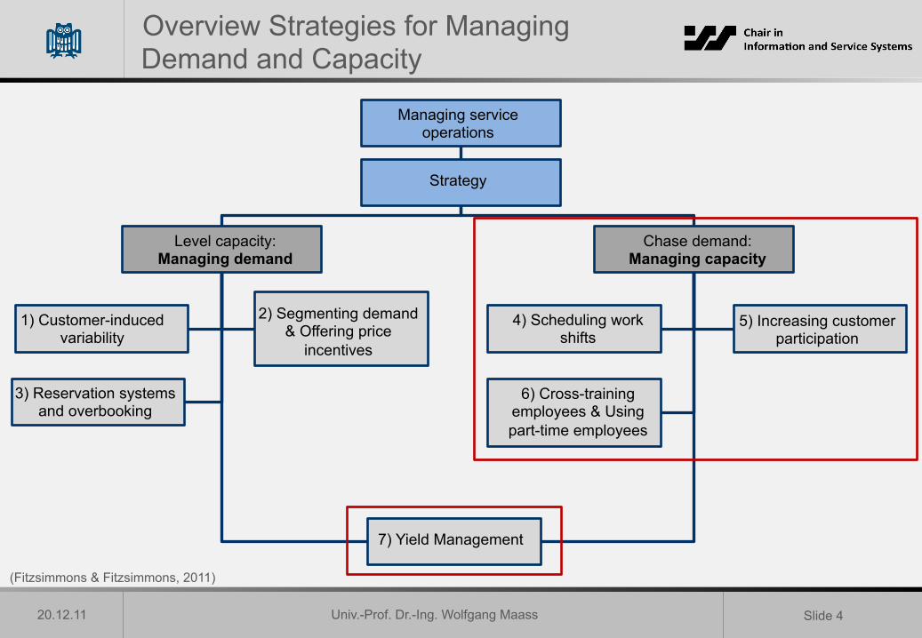
Overview Strategies for Managing Demand and Capacity
Managing service operations
Strategy
Level capacity: Managing demand
Chase demand: Managing capacity
7) Yield Management
1) Customer-induced variability
2) Segmenting demand & Offering price
incentives
3) Reservation systems and overbooking
6) Cross-training employees & Using part-time employees
5) Increasing customer participation
4) Scheduling work shifts
(Fitzsimmons & Fitzsimmons, 2011)

Univ.-Prof. Dr.-Ing. Wolfgang Maass
20.12.11 Slide 5
Agenda Lecture 8
• Overview Strategies for Managing Demand and Capacity • Managing Capacity
• Necessity • Scheduling work shifts • Increasing customer participation • Cross-training employees & Using part-time employees
• Managing Demand and Capacity: Yield Management
Univ.-Prof. Dr.-Ing. Wolfgang Maass
20.12.11 Slide 6
Managing Capacity: Necessity
• Service industry: Large variations in demand levels (e.g., in transportation, lodging or restaurant industry)
• Problem of some service companies: Demand cannot be allocated easily (e.g., 24-hour call center)
• Demand varies in short-terms • Demand varies due to time of day, week or season
• Demand cannot be adapted to capacity, but capacity needs to be adapted to demand.
• Financial success depends on management of productive capacity (e.g.,
personnel and equipment) to use them as efficiently as possible • Low demand: Productive capacity is wasted • High demand: Demand cannot be met as productive capacity is not
• Demand needs to be forecasted and capacity adopted accordingly.
(Buffa et al., 1976; Lovelock, 1984; Fitzsimmons & Fitzsimmons, 2011)

Univ.-Prof. Dr.-Ing. Wolfgang Maass
20.12.11 Slide 7
Agenda Lecture 8
• Overview Strategies for Managing Demand and Capacity • Managing Capacity
• Necessity • Scheduling work shifts • Increasing customer participation • Cross-training employees & Using part-time employees
• Managing Demand and Capacity: Yield Management

Univ.-Prof. Dr.-Ing. Wolfgang Maass
20.12.11 Slide 8
Managing Capacity: Scheduling work shifts
• Work shift scheduling: Scheduling employees to adopt to variable demand pattern (e.g., daily, weekly or seasonal variability).
• Example: 24 h telephone operator
• Service level: In 89% of the time incoming calls must be answered within 10 seconds.
• Difficulty: Strong variability of demand • Peak volume: 10:30-11:00 A.M. (2560 calls) • Minimum volume: 5:30 A.M. (20 calls)
• Steps of creating a work shift schedule • Forecasting demand • Convert to operator requirements • Schedule shifts • Assign operators to shifts
• Forecasting • Demand per day: Forecasted in half-hour intervals
including seasonal and weekly variations (lower demand at the weekend and in summer, high demand on Christmas)
• Exponential smoothing with seasonal adjustment used (e.g., last weeks forecasting error is included)
(Buffa et al., 1976)
622 DECISION SCIENCES
FIGURE 2 Daily call load for Long Beach, January 1972.
FIGURE 3 Typicat half-hourly call distribution (Bundy D A).
CALLS
1
[Vol. 7
calls per minute indicates that the standard deviation is equal to the square root of the mean, a reasonable, practical test for randomness, and that the arrival rates are described by the Poisson distribution. For the sample of Figure 4, R = 15.75 calls per minute; SD = 4.85 calls per minute; and 415.75 = 3.99. Therefore, the variation within the hour is taken as random. This variation can- not be accommodated by planning and scheduling, thus sufficient capacity must be provided to absorb the random variations.
__
Demand curve

Univ.-Prof. Dr.-Ing. Wolfgang Maass
20.12.11 Slide 9
Managing Capacity: Scheduling work shifts
• Schedule shifts • Shifts need to be assigned to the demand (adopt to
demand line): Computerized • Restrictions (shift is 7-8 hours, lunch break, days off, laws) • Di = Number of operators needed in period i • Wi = Number of operators assigned in period i Objective: Result: • List of optimum distribution of shifts & schedule of break
during shifts
• Assign operators to shifts (in exercise)
(Buffa et al., 1976)
19761 AN INTEGRATED W O R K SHIFT SCHEDULING SYSTEM 627
5 . Eight hour shifts end before 9 P.M. 6. Seven hour shifts end from 9:30 to 10:30 P.M. 7. Six and one-half hour shifts end at 11 :00 P.M. or later. 8. Earliest lunch period is at 1O:OO A.M. Luce [17] developed a heuristic algorithm for choosing shifts from the
approved set in such a way that the absolute differences between operators de- manded by the topline profile in period i , D i , and the operators provided, Wi , is minimized when summed over all n periods of the day, that is
n Minimize I Di - Wi I. (1)
i= l
The strategy is to build up the operator resources in the schedule, one shift at a time, drawing on the universal set of approved shifts. The criterion stated in (1) is used to choose shifts at each step. Conceptually, as the schedule of W i values is built up, the distance is minimized between the demand and operators sup- plied curves as illustrated by Figure 9.
At each stage in building up the schedule, there exists some remaining dis- tance between Di and Wi . The criterion for choice of the next shift is the fol- lowing test on each alternate shift: add the contributions of the shift to Wi (1 for all working periods and 0 for idle periods such as lunch and rest pauses), and recalculate expression (1). Choose the shift which minimizes (1). In order to negate the preference of the preceding choice rule to favor shorter length shifts, the different shift lengths are weighted in the calculation. The longest shift is given a weight of 1.0, and shorter shifts are weighted by the ratio of the working
FIGURE 9 Concept of the schedule building process, using the criterion, minimize ..
50
40 E
:: In 5 30 Y
P Y 0 a 20 m 5
10
0 , DEMAND b-[ ------ W, A T FINAL STAGE 1 . t - 9 3 7-m 9
1 1 1 1 1 1 1 1 1 1 1 1 1 1 1 2 3 4 5 6 7 8 9 10 11 12 13 14 15 16 17
TIME INTERVALS
• Convert to operator requirements • Number of operators required is calculated per half-hour • Total day operator hours must be allocated to the half-hour demand • Conventional queuing model is used (including exponential smoothing) • Result: Number of operators required per half-hour taking into account the response time (demand)

Univ.-Prof. Dr.-Ing. Wolfgang Maass
20.12.11 Slide 10
Agenda Lecture 8
• Overview Strategies for Managing Demand and Capacity • Managing Capacity
• Necessity • Scheduling work shifts • Increasing customer participation • Cross-training employees & Using part-time employees
• Managing Demand and Capacity: Yield Management
Univ.-Prof. Dr.-Ing. Wolfgang Maass
20.12.11 Slide 11
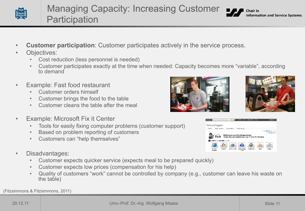
Managing Capacity: Increasing Customer Participation
• Customer participation: Customer participates actively in the service process. • Objectives:
• Cost reduction (less personnel is needed) • Customer participates exactly at the time when needed: Capacity becomes more “variable”, according
to demand
• Example: Fast food restaurant • Customer orders himself • Customer brings the food to the table • Customer cleans the table after the meal
• Example: Microsoft Fix it Center • Tools for easily fixing computer problems (customer support) • Based on problem reporting of customers • Customers can “help themselves”
• Disadvantages: • Customer expects quicker service (expects meal to be prepared quickly) • Customer expects low prices (compensation for his help) • Quality of customers “work” cannot be controlled by company (e.g., customer can leave his waste on
the table)
(Fitzsimmons & Fitzsimmons, 2011)

Univ.-Prof. Dr.-Ing. Wolfgang Maass
20.12.11 Slide 12
Brainteaser
• Think of 3 examples (besides fast-food restaurant) of customer participation in the service industry.
• How has the internet influenced customer participation in service processes?
• Please write your answers down (papers will be
collected for discussion in exercise).
10 Minutes

Univ.-Prof. Dr.-Ing. Wolfgang Maass
20.12.11 Slide 13
Agenda Lecture 8
• Overview Strategies for Managing Demand and Capacity • Managing Capacity
• Necessity • Scheduling work shifts • Increasing customer participation • Cross-training employees & Using part-time employees
• Managing Demand and Capacity: Yield Management
Univ.-Prof. Dr.-Ing. Wolfgang Maass
20.12.11 Slide 14
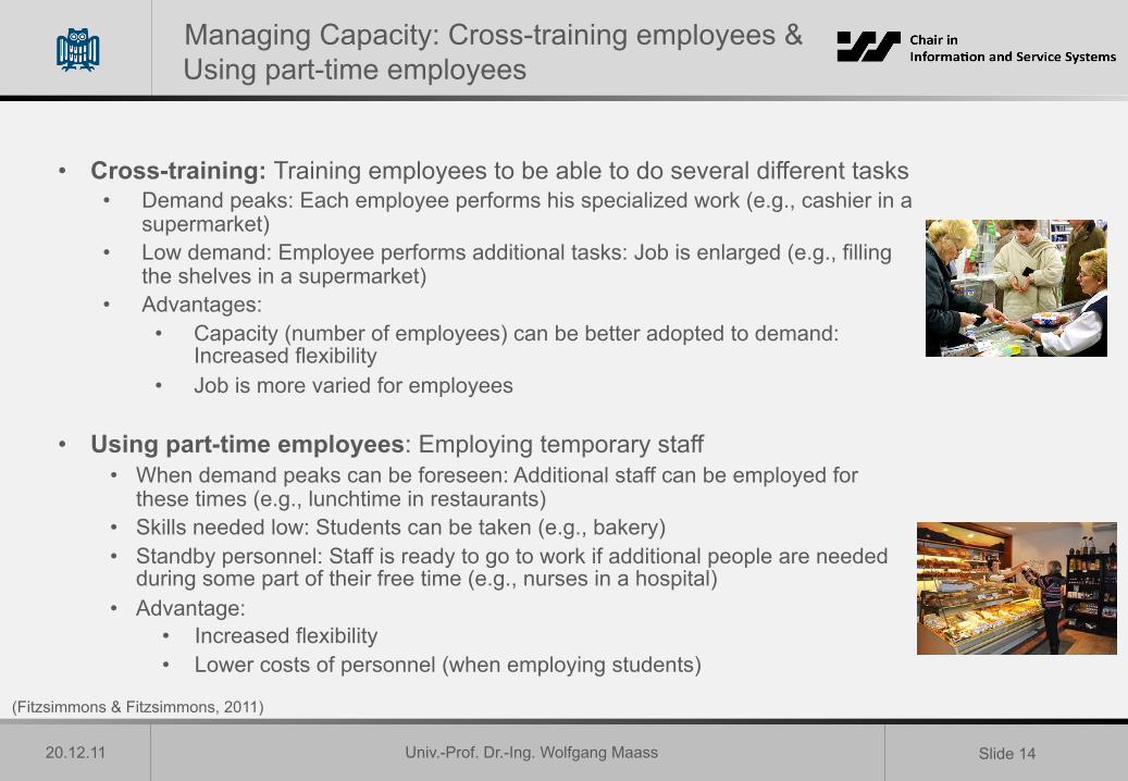
Managing Capacity: Cross-training employees & Using part-time employees
• Cross-training: Training employees to be able to do several different tasks • Demand peaks: Each employee performs his specialized work (e.g., cashier in a
supermarket) • Low demand: Employee performs additional tasks: Job is enlarged (e.g., filling
the shelves in a supermarket) • Advantages:
• Capacity (number of employees) can be better adopted to demand: Increased flexibility
• Job is more varied for employees
• Using part-time employees: Employing temporary staff • When demand peaks can be foreseen: Additional staff can be employed for
these times (e.g., lunchtime in restaurants) • Skills needed low: Students can be taken (e.g., bakery) • Standby personnel: Staff is ready to go to work if additional people are needed
during some part of their free time (e.g., nurses in a hospital) • Advantage:
• Increased flexibility • Lower costs of personnel (when employing students)
(Fitzsimmons & Fitzsimmons, 2011)

Univ.-Prof. Dr.-Ing. Wolfgang Maass
20.12.11 Slide 15
Agenda Lecture 8
• Overview Strategies for Managing Demand and Capacity • Managing Capacity
• Necessity • Scheduling work shifts • Increasing customer participation • Cross-training employees & Using part-time employees
• Managing Demand and Capacity: Yield Management

Univ.-Prof. Dr.-Ing. Wolfgang Maass
20.12.11 Slide 16
Managing Demand and Capacity: Yield Management
• Definition yield management: “(…) Yield management guides the decision of how to allocate undifferentiated units of capacity to available demand in such a way as to maximize profit or revenue.” (Kimes, 1989).
• “Yield management allows the airlines to allocate their fixed capacity of seats
in the most profitable manner possible.” (Kimes, 1989) • “(…) forecast demand and calculate the number of seats to be made available
to each fare type, with the goal of maximizing total flight revenues.“ (Belobaba et al., 1997)
• Problems of airlines:
• Airline’s inventory (seats) are of perishable nature: Empty seat is opportunity costs (high fixed capacity with high fixed costs).
• Airlines prefer filling their planes with full-fare customers, but often there are not enough of them (seats would remain empty).
• Low-fare passengers might take all of the seats and there will not be any left for full-fare passengers who book lately.
• Solution: Determination of how much of the capacity to sell at what price and to which market segment, especially amount of discount fares. Leaving enough capacity for late-booking full-fare customers (using yield management).
(Kimes, 1989, Belobaba et al., 1997)
First Class
Business Class
Economy Class
Univ.-Prof. Dr.-Ing. Wolfgang Maass
20.12.11 Slide 17
Managing Demand and Capacity: Yield Management
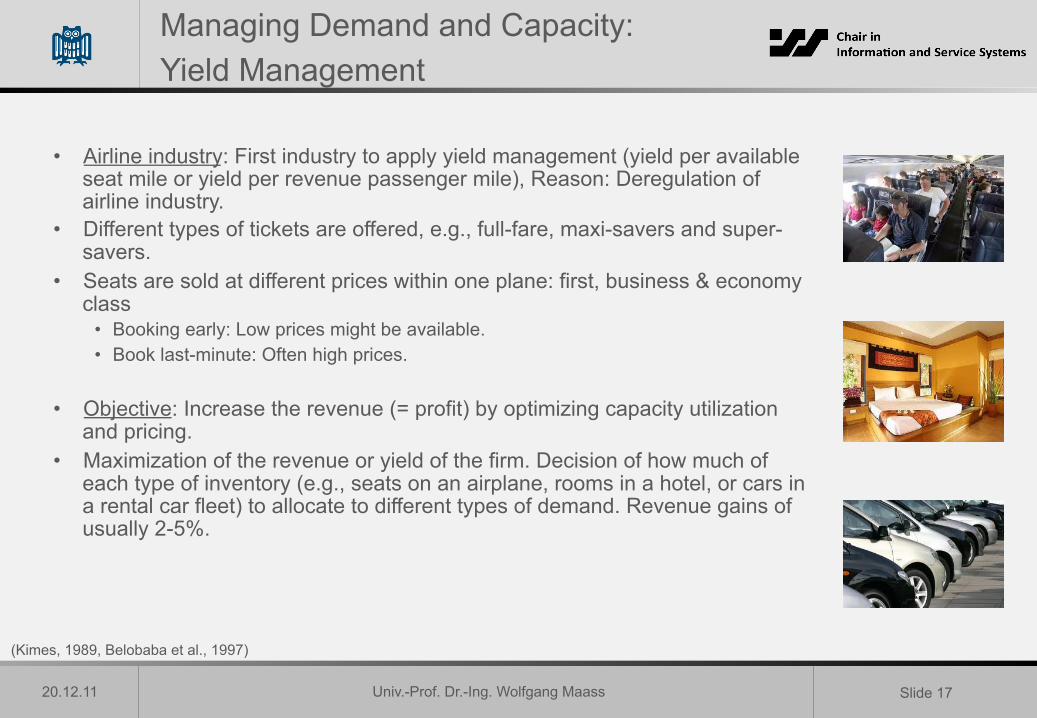
• Airline industry: First industry to apply yield management (yield per available seat mile or yield per revenue passenger mile), Reason: Deregulation of airline industry.
• Different types of tickets are offered, e.g., full-fare, maxi-savers and super-savers.
• Seats are sold at different prices within one plane: first, business & economy class
• Booking early: Low prices might be available. • Book last-minute: Often high prices.
• Objective: Increase the revenue (= profit) by optimizing capacity utilization and pricing.
• Maximization of the revenue or yield of the firm. Decision of how much of each type of inventory (e.g., seats on an airplane, rooms in a hotel, or cars in a rental car fleet) to allocate to different types of demand. Revenue gains of usually 2-5%.
(Kimes, 1989, Belobaba et al., 1997)

Univ.-Prof. Dr.-Ing. Wolfgang Maass
20.12.11 Slide 18
Managing Demand and Capacity: Yield Management
• Trade-off: Between high capacity utilization and selling seats at maximum price. • Especially used in capital-intensive service industries (airlines, hotels, car-rentals & cruise
lines) with high fixed costs and much lower variable costs. • If fixed costs are covered: Marginal costs of selling another seat are small compared to the
marginal revenue. • Characteristics of industries convenient for yield management:
• Relatively fixed capacity (high fixed costs for a hotel & employees) • Demand can be segmented into clearly-identified partitions (e.g., business customers vs. tourists in a hotel) • Inventory is perishable (e.g., empty seats on a plane) • Product is sold some time in advance (e.g., tickets for a cruise) • Demand fluctuates strongly (e.g., according to day of the week or season) • Marginal sales costs and production costs are low, but capacity costs are high (e.g., costs of a cruising ship &
crew are high, but variable costs for 1 additional passenger are low).
• Managers need to detect the different customer’s needs, segment the market accordingly & identify the patterns in demand’s fluctuation.
• Yield management system: Combines seat inventory management with pricing tools and
demand forecasting methods.
(Kimes, 1989; Lovelock, 1984)

Univ.-Prof. Dr.-Ing. Wolfgang Maass
20.12.11 Slide 19
Demand-capacity conditions of service companies:
1. Demand exceeds maximum available capacity: Potential business may be lost (e.g., overbooking of hotels)
2. Demand exceeds the optimum capacity level: No customer is turned away, but quality of delivered service is reduced for all customers (e.g., crowded bus, restaurant where every table is occupied).
3. Demand and supply are well balanced at the level of optimum capacity (optimum, objective that should be reached).
4. Demand is below optimum capacity and resources are under-utilised: Waste of resources (e.g., staff at a car repair shop is bored as there are too few customers).
Example: Hotel allocates a certain percentage of its rooms to different customer segments during different seasons (charges multiple prices) (Lovelock, 1984)
Managing Demand and Capacity: Yield Management
Percentage of capacity allocated to different seasons
Percentage of capacity allocated to different segments
Peak (30%), e.g., summer
1st shoulder (20%), e.g., spring
Off-peak (40%), e.g., winter
2nd shoulder (10%), e.g., fall
10%
50%
30% 20% 20% 20%
50% 30%
50%
30%
50%
30%
First class
Standard
Budget
Univ.-Prof. Dr.-Ing. Wolfgang Maass
20.12.11 Slide 20
Managing Demand and Capacity: Yield Management
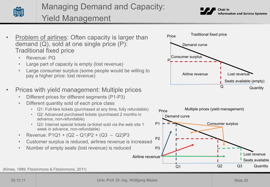
• Problem of airlines: Often capacity is larger than demand (Q), sold at one single price (P): Traditional fixed price
• Revenue: PQ • Large part of capacity is empty (lost revenue) • Large consumer surplus (some people would be willing to
pay a higher price: lost revenue)
• Prices with yield management: Multiple prices • Different prices for different segments (P1-P3) • Different quantity sold of each price class
• Q1: Full-fare tickets (purchased at any time, fully refundable) • Q2: Advanced purchased tickets (purchased 2 months in
advance, non-refundable) • Q3: Internet special tickets (e-ticket sold via the web site 1
week in advance, non-refundable) • Revenue: P1Q1 + (Q2 – Q1)P2 + (Q3 – Q2)P3 • Customer surplus is reduced, airlines revenue is increased • Number of empty seats (lost revenue) is reduced
(Kimes, 1989; Fitzsimmons & Fitzsimmons, 2011)
Price Traditional fixed price
P
Quantity Q
Demand curve
Consumer surplus
Airline revenue
Seats available (empty)
Lost revenue
Price Multiple prices (yield management)
P1
Quantity Q2
Demand curve
Consumer surplus
Seats available
P3
P2
Q1 Q3
Lost revenue Airline revenue
Univ.-Prof. Dr.-Ing. Wolfgang Maass
20.12.11 Slide 21
Managing Demand and Capacity: Yield Management
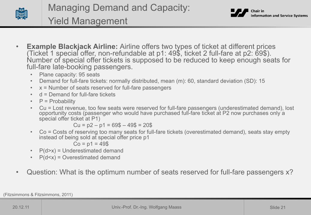
• Example Blackjack Airline: Airline offers two types of ticket at different prices (Ticket 1 special offer, non-refundable at p1: 49$, ticket 2 full-fare at p2: 69$). Number of special offer tickets is supposed to be reduced to keep enough seats for full-fare late-booking passengers.
• Plane capacity: 95 seats • Demand for full-fare tickets: normally distributed, mean (m): 60, standard deviation (SD): 15 • x = Number of seats reserved for full-fare passengers • d = Demand for full-fare tickets • P = Probability • Cu = Lost revenue, too few seats were reserved for full-fare passengers (underestimated demand), lost
opportunity costs (passenger who would have purchased full-fare ticket at P2 now purchases only a special offer ticket at P1)
Cu = p2 – p1 = 69$ – 49$ = 20$ • Co = Costs of reserving too many seats for full-fare tickets (overestimated demand), seats stay empty
instead of being sold at special offer price p1 Co = p1 = 49$
• P(d>x) = Underestimated demand • P(d<x) = Overestimated demand
• Question: What is the optimum number of seats reserved for full-fare passengers x?
(Fitzsimmons & Fitzsimmons, 2011)
Univ.-Prof. Dr.-Ing. Wolfgang Maass
20.12.11 Slide 22
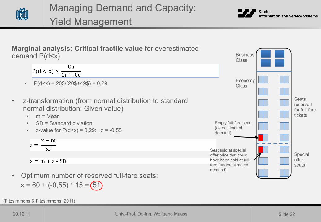
Managing Demand and Capacity: Yield Management
Marginal analysis: Critical fractile value for overestimated demand P(d<x)
• P(d<x) = 20$/(20$+49$) = 0,29 • z-transformation (from normal distribution to standard
normal distribution: Given value) • m = Mean • SD = Standard diviation • z-value for P(d<x) = 0,29: z = -0,55
• Optimum number of reserved full-fare seats:
x = 60 + (-0,55) * 15 = 51
(Fitzsimmons & Fitzsimmons, 2011)
Business Class
Economy Class
Seats reserved for full-fare tickets
Special offer seats
Empty full-fare seat (overestimated demand)
Seat sold at special offer price that could have been sold at full-fare (underestimated demand)
Univ.-Prof. Dr.-Ing. Wolfgang Maass
20.12.11 Slide 23
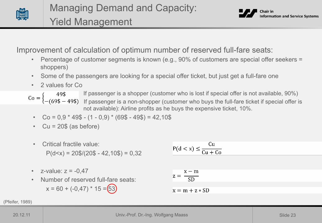
Managing Demand and Capacity: Yield Management
Improvement of calculation of optimum number of reserved full-fare seats: • Percentage of customer segments is known (e.g., 90% of customers are special offer seekers =
shoppers) • Some of the passengers are looking for a special offer ticket, but just get a full-fare one • 2 values for Co
• If passenger is a shopper (customer who is lost if special offer is not available, 90%) If passenger is a non-shopper (customer who buys the full-fare ticket if special offer is not available): Airline profits as he buys the expensive ticket, 10%.
• Co = 0,9 * 49$ - (1 - 0,9) * (69$ - 49$) = 42,10$ • Cu = 20$ (as before)
• Critical fractile value: P(d<x) = 20$/(20$ - 42,10$) = 0,32
• z-value: z = -0,47 • Number of reserved full-fare seats:
x = 60 + (-0,47) * 15 = 53
(Pfeifer, 1989)

Univ.-Prof. Dr.-Ing. Wolfgang Maass
20.12.11 Slide 24
Outlook
1. Introduction 2. Service Strategy 3. New Service Development (NSD) 4. Service Quality 5. Supporting Facility 6. Forecasting Demand for Services 7. Managing Demand 8. Managing Capacity 9. Managing Waiting Lines 10. Capacity Planning and Queuing Models 11. Services and Information Systems 12. ITIL Service Design 13. IT Service Infrastructures 14. Guest Lecture – Dr. Roehn, Deutsche Telekom 15. Summary and Outlook

Univ.-Prof. Dr.-Ing. Wolfgang Maass
20.12.11 Slide 25
Literature
Books: • Fitzsimmons, J. A. & Fitzsimmons, M. J. (2011), Service Management - Operations, Strategy, Information Technology,
McGraw – Hill.
Papers: • Belobaba, P.P. & Wilson, J.L. (1997), “Impacts of Yield Management in Competitive Airline Markets”, Journal of Air Transport
Management, 3(1), pp. 3-9. • Buffa, E.S., Cosgrove, M.J. & Luce, B.J. (1976), “An Integrated Work Shift Scheduling System”, Decision Sciences, 7(4), pp.
620-630. • Kimes, S.H. (1989), “Yield Management: A Too for Capacity-Constrained Service Firms”, Journal of Operations Management,
8(4), pp. -363. • Lovelock, C.H.(1984), “Strategies for Managing Demand in Capacity-Constrained Service Organisations”, The Service
Industries Journal, 4(3), pp. 12-30. • Pfeifer, P.E. (1989), “The Airline Discount Fare Allocation Problem“, Decision Sciences, 20(1), pp. 149-157.

Univ.-Prof. Dr.-Ing. Wolfgang Maass
Univ.-Prof. Dr.-Ing. Wolfgang Maass Chair in Information and Service Systems Saarland University, Germany