service life modeling of virginia bridge … · a bridge deck and then a corrosion propagation time...

SERVICE LIFE MODELING OF VIRGINIA BRIDGE DECKS

by

Gregory Williamson

Dissertation submitted to the faculty of the

Virginia Polytechnic Institute and State University

in partial fulfillment of the requirements for the degree of

Doctor of Philosophy

in

Civil & Environmental Engineering

Committee Members Richard E. Weyers, Chair

Carin L. Roberts-Wollmann Jack Lesko

Michael C. Brown Michael Sprinkel

March 20, 2007

Blacksburg, Virginia Keywords: corrosion, concrete, bridge deck, service life, life-cycle cost analysis, chloride

diffusion

Copyright 2007, Gregory S. Williamson

SERVICE LIFE MODELING OF VIRGINIA BRIDGE DECKS

Gregory Williamson

ABSTRACT

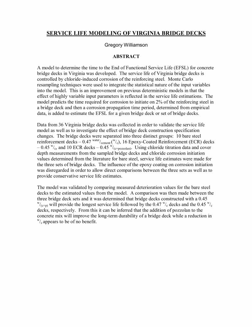
A model to determine the time to the End of Functional Service Life (EFSL) for concrete bridge decks in Virginia was developed. The service life of Virginia bridge decks is controlled by chloride-induced corrosion of the reinforcing steel. Monte Carlo resampling techniques were used to integrate the statistical nature of the input variables into the model. This is an improvement on previous deterministic models in that the effect of highly variable input parameters is reflected in the service life estimations. The model predicts the time required for corrosion to initiate on 2% of the reinforcing steel in a bridge deck and then a corrosion propagation time period, determined from empirical data, is added to estimate the EFSL for a given bridge deck or set of bridge decks. Data from 36 Virginia bridge decks was collected in order to validate the service life model as well as to investigate the effect of bridge deck construction specification changes. The bridge decks were separated into three distinct groups: 10 bare steel reinforcement decks � 0.47 water/cement (w/c), 16 Epoxy-Coated Reinforcement (ECR) decks � 0.45 w/c, and 10 ECR decks � 0.45 w/(c+pozzolan). Using chloride titration data and cover depth measurements from the sampled bridge decks and chloride corrosion initiation values determined from the literature for bare steel, service life estimates were made for the three sets of bridge decks. The influence of the epoxy coating on corrosion initiation was disregarded in order to allow direct comparisons between the three sets as well as to provide conservative service life estimates. The model was validated by comparing measured deterioration values for the bare steel decks to the estimated values from the model. A comparison was then made between the three bridge deck sets and it was determined that bridge decks constructed with a 0.45 w/(c+p) will provide the longest service life followed by the 0.47 w/c decks and the 0.45 w/c decks, respectively. From this it can be inferred that the addition of pozzolan to the concrete mix will improve the long-term durability of a bridge deck while a reduction in w/c appears to be of no benefit.

iii

ACKNOWLEDGEMENTS

I would first like to express my gratitude to Dr. Richard E. Weyers for his constant guidance while serving as my graduate advisor. His support, encouragement, and mentorship throughout my graduate work are very much appreciated. I would also like to thank the members of my doctoral committee, Dr. Michael Brown, Dr. Jack Lesko, Dr. Carin Roberts-Wollmann, and Mr. Michael Sprinkel, who have provided their insight and expertise to this study. I would like to offer my sincere thanks to the National Science Foundation, Via Endowment Program, Virginia Transportation Research Council, and Virginia Polytechnic Institute who provided the financial support for this research project. Many thanks are owed to my fellow graduate students whose friendship has made my graduate experience much more enjoyable. I owe special thanks to Andrei Ramniceanu for his assistance in gathering field data. I would also like to express my appreciation to Brett Farmer and Dennis Huffman for their technical assistance, humor, and friendship during my time spent at the Structures Lab. Finally, I thank my wife Amy. Her unwavering love and support have sustained me throughout this incredible endeavor. Lastly, I would like to thank my mother and hero Valerie Rose, who has sacrificed so much to provide me with the opportunity to pursue my graduate work, without the work ethic, determination, and commitment to excellence that she instilled in me, this work would not have been possible.

iv

TABLE OF CONTENTS INTRODUCTION 1

BACKGROUND 2

LITERATURE REVIEW 3

Corrosion of Steel in Concrete 3

Chloride Induced Corrosion 4

Carbonation Induced Corrosion 5

Corrosion of Bare Steel in Concrete 6

Corrosion of Epoxy-Coated Steel in Concrete 6

Chloride Threshold Concentrations 7

Time to Corrosion-Induced Cracking of Cover Concrete 9

Deck Protection, Repair, and Rehabilitation Methods 9

Deck Protection Methods 10

Deck Sealers 10

Cathodic Prevention 11

Stainless Steel Reinforcement 11

Galvanized Steel Reinforcement 14

Epoxy-Coated Reinforcement 15

MMFX Reinforcement 16

Corrosion Inhibitors 16

Improved Concrete Properties 18

Deck Repair Methods 19

Patching 19

Deck Overlays 20

Deck Rehabilitation Methods 20

Deck Overlays 21

Cathodic Protection 21

v

Chloride Diffusion Models 21

Fickian Diffusion 22

Effect of Time-Dependent Diffusion Coefficients 23

Effect of Time-Dependent Surface Chloride Concentrations 24

Effect of Pozzolans 25

Effect of Chloride Binding 26

Fickian Diffusion Models 28

Cady and Weyers 28

Mangat and Molloy 28

Maheswaran and Sanjayan 30

Bamforth 30

Limitations of Proposed Models 31

Finite Element Method (FEM) Modeling of Diffusion 32

FEM Diffusion Models 33

Saetta, Scotta, and Vitaliani 33

Boddy, Bentz, Thomas, and Hooten 34

Martín-Pérez, Pantazopoulou, and Thomas 36

Commercially Available Models 36

STADIUM 36

Life 365 38

Corrosion Induced Cracking of Concrete Cover 40

Corrosion Cracking Models 41

Ba�ant 41

Liu/Weyers 43

Alonso, Andrade, Rodriguez, and Diez 45

Torres-Acosta/Sagüés 46

Vu, Stewart, and Mullard 47

Finite Element Analysis of Corrosion Induced Crack Propagation 49

OBJECTIVE 50

vi

SCOPE 51

METHODS AND MATERIALS 52

Bridge Deck Selection 52

Deck Survey 54

Visual Survey 55

Non-destructive Field Testing 55

Deck Cores and Laboratory Testing 56

METHOD OF ANALYSIS 57

Service Life Model 57

Deterministic vs. Probabilistic Service Life Models 59

Monte Carlo Simulation 59

Parametric Bootstrapping 60

Simple Bootstrapping 60

Modeling the Time to Corrosion Initiation 60

Apparent Diffusion Coefficient Calculation 60

Background Chloride Concentration Determination 63

Adjusting Diffusion Coefficients for Time Dependency 65

BCA Service Life Model 69

Estimating the Time to Corrosion Cracking for Bare Steel 74

Estimating the Time to Corrosion Cracking for ECR 76

Estimating the Propagation Time of Corrosion for Bare Steel Bridge Decks 76

Estimating the Propagation Time of Corrosion for ECR Bridge Decks 78

Simulation Input Data 79

Chloride Threshold Concentrations 79

Apparent Diffusion Coefficients (Dca) 80

Surface Chloride Concentrations (Co) 81

Cover Depths (x) 81

vii

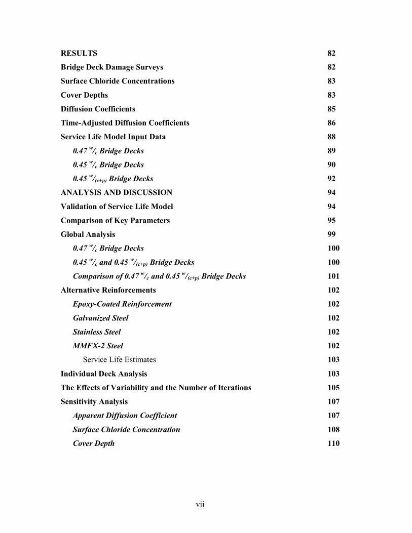
RESULTS 82

Bridge Deck Damage Surveys 82

Surface Chloride Concentrations 83

Cover Depths 83

Diffusion Coefficients 85

Time-Adjusted Diffusion Coefficients 86

Service Life Model Input Data 88

0.47 w/c Bridge Decks 89


0.45 w/(c+p) Bridge Decks 92

ANALYSIS AND DISCUSSION 94

Validation of Service Life Model 94

Comparison of Key Parameters 95

Global Analysis 99


0.45 w/c and 0.45 w/(c+p) Bridge Decks 100

Comparison of 0.47 w/c and 0.45 w/(c+p) Bridge Decks 101

Alternative Reinforcements 102

Epoxy-Coated Reinforcement 102

Galvanized Steel 102

Stainless Steel 102

MMFX-2 Steel 102

Service Life Estimates 103

Individual Deck Analysis 103

The Effects of Variability and the Number of Iterations 105

Sensitivity Analysis 107

Apparent Diffusion Coefficient 107

Surface Chloride Concentration 108

Cover Depth 110

viii

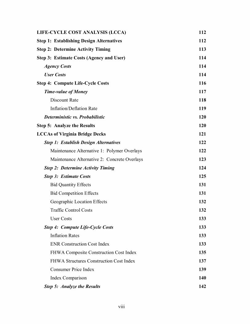
LIFE-CYCLE COST ANALYSIS (LCCA) 112

Step 1: Establishing Design Alternatives 112

Step 2: Determine Activity Timing 113

Step 3: Estimate Costs (Agency and User) 114

Agency Costs 114

User Costs 114

Step 4: Compute Life-Cycle Costs 116

Time-value of Money 117

Discount Rate 118

Inflation/Deflation Rate 119

Deterministic vs. Probabilistic 120

Step 5: Analyze the Results 120

LCCAs of Virginia Bridge Decks 121

Step 1: Establish Design Alternatives 122

Maintenance Alternative 1: Polymer Overlays 122

Maintenance Alternative 2: Concrete Overlays 123

Step 2: Determine Activity Timing 124

Step 3: Estimate Costs 125

Bid Quantity Effects 131

Bid Competition Effects 131

Geographic Location Effects 132

Traffic Control Costs 132

User Costs 133

Step 4: Compute Life-Cycle Costs 133

Inflation Rates 133

ENR Construction Cost Index 133

FHWA Composite Construction Cost Index 135

FHWA Structures Construction Cost Index 137

Consumer Price Index 139

Index Comparison 140

Step 5: Analyze the Results 142

ix

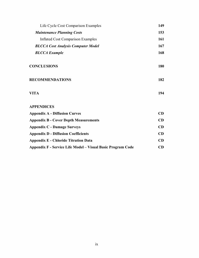
Life Cycle Cost Comparison Examples 149

Maintenance Planning Costs 153

Inflated Cost Comparison Examples 161

BLCCA Cost Analysis Computer Model 167

BLCCA Example 168

CONCLUSIONS 180

RECOMMENDATIONS 182

VITA 194

APPENDICES

Appendix A - Diffusion Curves CD

Appendix B - Cover Depth Measurements CD

Appendix C - Damage Surveys CD

Appendix D - Diffusion Coefficients CD

Appendix E - Chloride Titration Data CD

Appendix F - Service Life Model � Visual Basic Program Code CD

x

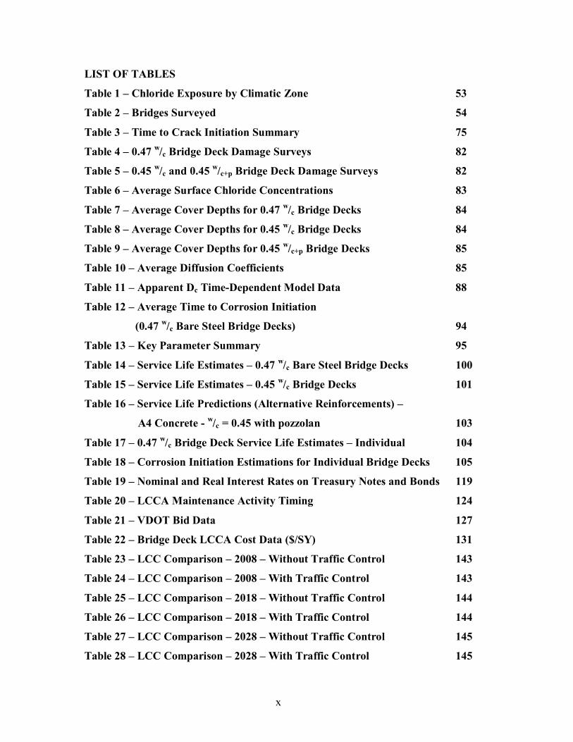
LIST OF TABLES

Table 1 � Chloride Exposure by Climatic Zone 53

Table 2 � Bridges Surveyed 54

Table 3 � Time to Crack Initiation Summary 75

Table 4 � 0.47 w/c Bridge Deck Damage Surveys 82

Table 5 � 0.45 w/c and 0.45 w/c+p Bridge Deck Damage Surveys 82

Table 6 � Average Surface Chloride Concentrations 83

Table 7 � Average Cover Depths for 0.47 w/c Bridge Decks 84

Table 8 � Average Cover Depths for 0.45 w/c Bridge Decks 84

Table 9 � Average Cover Depths for 0.45 w/c+p Bridge Decks 85

Table 10 � Average Diffusion Coefficients 85

Table 11 � Apparent Dc Time-Dependent Model Data 88

Table 12 � Average Time to Corrosion Initiation

(0.47 w/c Bare Steel Bridge Decks) 94

Table 13 � Key Parameter Summary 95

Table 14 � Service Life Estimates � 0.47 w/c Bare Steel Bridge Decks 100

Table 15 � Service Life Estimates � 0.45 w/c Bridge Decks 101

Table 16 � Service Life Predictions (Alternative Reinforcements) �

A4 Concrete - w/c = 0.45 with pozzolan 103

Table 17 � 0.47 w/c Bridge Deck Service Life Estimates � Individual 104

Table 18 � Corrosion Initiation Estimations for Individual Bridge Decks 105

Table 19 � Nominal and Real Interest Rates on Treasury Notes and Bonds 119

Table 20 � LCCA Maintenance Activity Timing 124

Table 21 � VDOT Bid Data 127

Table 22 � Bridge Deck LCCA Cost Data ($/SY) 131

Table 23 � LCC Comparison � 2008 � Without Traffic Control 143

Table 24 � LCC Comparison � 2008 � With Traffic Control 143





xi







Table 35 � LCCA � Example 1 149



Table 38 � Inflated Cost Comparison � 2008 � Without TC 155

Table 39 � Inflated Cost Comparison � 2008 � With TC 155











Table 50 � Maintenance Activity Timings � Total Costs 161

Table 51 � Inflated Costs � Example 1 162



Table 54 � LCCA/Total Inflated Cost Comparison 167

Table 55 � ADT Primary Model 170

Table 56 � Condition Index Primary Model 170

Table 57 � Load Capacity Primary Model 170

Table 58 � Agency Maintenance Costs 171

Table 59 � Alternative 1 Event Timeline 172

xii

Table 60 � Condition Index � Polymer Overlay Redefined 173

Table 61 � User Costs � Polymer Overlays 174

Table 62 � Alternative 2 Event Timeline 175

Table 63 � Condition Index � Concrete Overlay Redefined 176

Table 64 � User Costs � Concrete Overlays 176

xiii

LIST OF FIGURES

Figure 1 � Chloride-Induced Corrosion Process 5

Figure 2 � Corrosion-Induced Cracking 40

Figure 3 � Surveyed Bridge Locations 52

Figure 4 � Virginia Climatic Zones 53

Figure 5 � Service Life Model 57

Figure 6 � Seasonal Fluctuations in Chloride Profiles 61

Figure 7 � Determination of Apparent Diffusion Coefficient 62

Figure 8 � BCA GUI � Dca Input Form 62

Figure 9 � BCA Output � Dca 63

Figure 10 � Background Chloride Concentration Determination Example 65

Figure 11 � Diffusion Decay � Mangat and Molloy 67

Figure 12 � Diffusion Decay � Bamforth 67

Figure 13 � Diffusion Decay � Life-365 68

Figure 14 � BCA GUI � Service Life Input Form 69

Figure 15 � BCA Chloride Threshold Input Form 71

Figure 16 � BCA Service Life Estimation Routine 73

Figure 17 � BCA Service Life CDF 73

Figure 18 � Corrosion Propagation Rates 77

Figure 19 � Total Propagation Time 77

Figure 20 � Corrosion Initiation Concentrations � Bare Steel 79

Figure 21 � Corrosion Initiation Concentrations

(Bare Steel � Randomly Generated) 80

Figure 22 � Apparent Dc Time-Dependency Model � Bamforth 86

Figure 23 � Apparent Dc Time-Dependency Model � Life 365 87

Figure 24 � Apparent Dc Time-Dependency Model � Mangat and Molloy 87

Figure 25 � Co Measurments � 0.47 w/c 89

Figure 26 � Diffusion Coefficients � 0.47 w/c 89

Figure 27 � Cover Depth Measurements � 0.47 w/c 90

Figure 28 � Surface Chloride Concentrations � 0.45 w/c No Pozzolan 90

Figure 29 � Cover Depth Measurements � 0.45 w/c No Pozzolan 91

xiv

Figure 30 � Diffusion Coefficients � 0.45 w/c No Pozzolan 91

Figure 31 � Surface Chloride Concentrations � 0.45 w/c With Pozzolan 92

Figure 32 � Cover Depth Measurements � 0.45 w/c With Pozzolan 92

Figure 33 � Diffusion Coefficients � 0.45 w/c With Pozzolan 93

Figure 34 � Dca Comparison � 0.45 No Pozz. to 0.45 With Pozz. 95

Figure 35 � Dca Comparison � 0.45 With Pozz. to 0.47 No Pozz 96

Figure 36 � Dca Comparison � 0.47 No Pozz. to 0.45 No Pozz 96

Figure 37 � Co Comparison � 0.45 No Pozz. to 0.45 With Pozz. 97

Figure 38 � Co Comparison � 0.45 With Pozz. to 0.47 No Pozz. 97

Figure 39 � Co Comparison � 0.47 No Pozz. to 0.45 No Pozz. 98

Figure 40 � Cover Depth Comparison � 0.47 No Pozz. to 0.45 With Pozz. 98

Figure 41 � Cover Depth Comparison � 0.45 With Pozz. to 0.45 No Pozz. 99

Figure 42 � Cover Depth Comparison � 0.45 No Pozz. to 0.47 No Pozz. 99

Figure 43 � Iteration Analysis for 0.47 w/c Bridge Deck Set 106

Figure 44 � Apparent Diffusion Coefficient vs. Time to Corrosion Initiation 107

Figure 45 � Surface Chloride Concentration vs. Time to Corrosion Initiation 109

Figure 46 � Cover Depth vs. Time to Corrosion Initiation 110

Figure 47 � VDOT Bid Data � Deck Patching � Type B 128

Figure 48 � VDOT Bid Data � Polymer Overlays 128

Figure 49 � VDOT Bid Data � Milling � Type A 129

Figure 50 � VDOT Bid Data � MSC/LMC Overlays 129

Figure 51 � VDOT Bid Data � Bridge Deck Grooving 130

Figure 52 � ENR Construction Cost Index 134

Figure 53 � CCI Average Annual Inflation Rate 135

Figure 54 � FHWA Composite CCI 136

Figure 55 � FHWA Composite CCI � Average Inflation Rate 137

Figure 56 � FHWA Structures CCI 138

Figure 57 � FHWA Structures CCI � Average Inflation Rate 138

Figure 58 � CPI 140

Figure 59 � CPI � Average Inflation Rate 140

Figure 60 � Index Comparison 141

xv

Figure 61 � Cash Flow Diagram � Example 5 153

Figure 62 � Cash Flow Diagram � Inflated Costs � Example 5 166

Figure 63 � Present Value During Event Costs � Alternative 1 �

Polymer Overlays 177

Figure 64 � Present Value During Event Costs � Alternative 2 �

Concrete Overlays 177

Figure 65 � Cumulative During Event Costs � Alternative 1 �

Polymer Overlays 178

Figure 66 � Cumulative During Event Costs � Alternative 2 �

Concrete Overlays 178

Figure 67 � Discount Rate Sensitivity Analysis 179

1

INTRODUCTION Bridge deck rehabilitation and replacement costs contribute significantly to the overall

state transportation budget in Virginia. Federal Highway Administration (FHWA) report

# RD-01-156 estimates the total direct costs of corrosion for highway bridges in the

United States to be $8.3 billion dollars per year, approximately half of which can be

attributed to superstructure deterioration. (FHWA, 2002) In addition to the direct costs

associated with maintaining the integrity of Virginia�s bridge system there are also

immeasurable impacts on the local economy due to interruptions in the flow of traffic

related to bridge closures. According to the 2004 National Bridge Inventory (NBI)

compiled by FHWA, 1,186 of Virginia�s 13,160 bridges (9%) are currently considered

structurally deficient. (FHWA, 2004) Bridges may be considered structurally deficient

for several reasons, for example excessive settlement or scour. However, the principal

cause of structural deterioration is related to the corrosion of the concrete reinforcing

steel. For this reason, being able to accurately model and predict the corrosion of the

reinforcement in bridge decks is of considerable interest to Virginia Department of

Transportation (VDOT) bridge engineers.

2

BACKGROUND

Corrosion of reinforcing steel in bridge decks can be initiated by one of two modes,

chloride-induced corrosion or carbonation-induced corrosion. To understand the

different modes of corrosion and the reasons for corrosion initiation one must first

understand the nature of steel in concrete. Steel when placed in an alkaline environment

such as concrete pore water, will develop a passive layer of corrosion products. This

passive layer is composed of iron oxides/hydroxides and is very dense. Over time this

passive layer will reach a thickness sufficient to protect the base metal and the corrosion

rate will for all practical purposes be equal to zero. As long as the passive layer remains

intact active corrosion will not initiate, however, if the reinforcing steel is depassivated

active corrosion can initiate and continue to propagate.

3

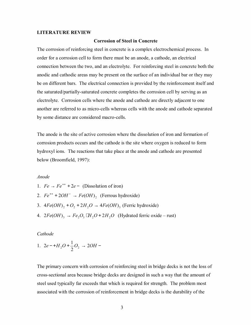
LITERATURE REVIEW

Corrosion of Steel in Concrete

The corrosion of reinforcing steel in concrete is a complex electrochemical process. In

order for a corrosion cell to form there must be an anode, a cathode, an electrical

connection between the two, and an electrolyte. For reinforcing steel in concrete both the

anodic and cathodic areas may be present on the surface of an individual bar or they may

be on different bars. The electrical connection is provided by the reinforcement itself and

the saturated/partially-saturated concrete completes the corrosion cell by serving as an

electrolyte. Corrosion cells where the anode and cathode are directly adjacent to one

another are referred to as micro-cells whereas cells with the anode and cathode separated

by some distance are considered macro-cells.

The anode is the site of active corrosion where the dissolution of iron and formation of

corrosion products occurs and the cathode is the site where oxygen is reduced to form

hydroxyl ions. The reactions that take place at the anode and cathode are presented

below (Broomfield, 1997):

Anode

1. −+→ ++ eFeFe 2 (Dissolution of iron)

2. 2)(2 OHFeOHFe →+ −++ (Ferrous hydroxide)

3. 3222 )(42)(4 OHFeOHOOHFe →++ (Ferric hydroxide)

4. OHOHOFeOHFe 22323 2)(2 +⋅→ (Hydrated ferric oxide � rust)

Cathode

1. −→++− OHOOHe 2212 22

The primary concern with corrosion of reinforcing steel in bridge decks is not the loss of

cross-sectional area because bridge decks are designed in such a way that the amount of

steel used typically far exceeds that which is required for strength. The problem most

associated with the corrosion of reinforcement in bridge decks is the durability of the

4

surrounding concrete. As corrosion progresses and iron reacts to form ferric oxides a

significant volume change takes place. The volume change (200 � 1000%) associated

with the corrosion process results in a buildup of pressure at the concrete/reinforcement

interface, which will ultimately result in the cracking, spalling, and delaminating of the

concrete cover. (Broomfield, 1997)

Chloride-Induced Corrosion

Corrosion of reinforcing steel in bridge decks is primarily associated with the diffusion of

chlorides into the concrete. Chloride ingress into concrete is the result of the application

of chloride bearing deicing salts, exposure to sea or brackish water, and to a lesser degree

the wind transport of salt water in coastal regions. Chlorides that are deposited on the

surface of the bridge deck will diffuse through the porous concrete and in time reach the

depth of the reinforcing steel. It should be noted, however, that while the ingress of

chlorides is typically modeled as strictly a diffusion process it is in actuality a much more

complex process. The initial movement of chlorides at the surface of the concrete can be

affected by capillary suction depending upon the percent saturation of the concrete.

Additionally, the chlorides once present within the concrete have the potential to bind

with aluminates and can also be affected by the fluxes of other ionic species. Due to the

complexity of these processes and their strong dependence upon the chemical

composition of the cement paste and pore water, their effects are generally ignored. It is

also important to note that by fitting a diffusion curve to chloride profiles all contributing

factors are accounted for whether they are diffusion related or not.

When the chlorides diffuse to the depth of the reinforcing steel they begin to attack the

passive layer of corrosion products present on the surface of the steel. The chloride

attack on the passive layer will not result in a decrease in pH, therefore, the passive layer

will continually reestablish itself. For low chloride concentrations the passive layer is

able to sustain itself and prevent active corrosion. However, when the concentration of

the chlorides at the reinforcement reaches a critical level the passive layer on the steel

reinforcement surface will break down and active corrosion will initiate.

5

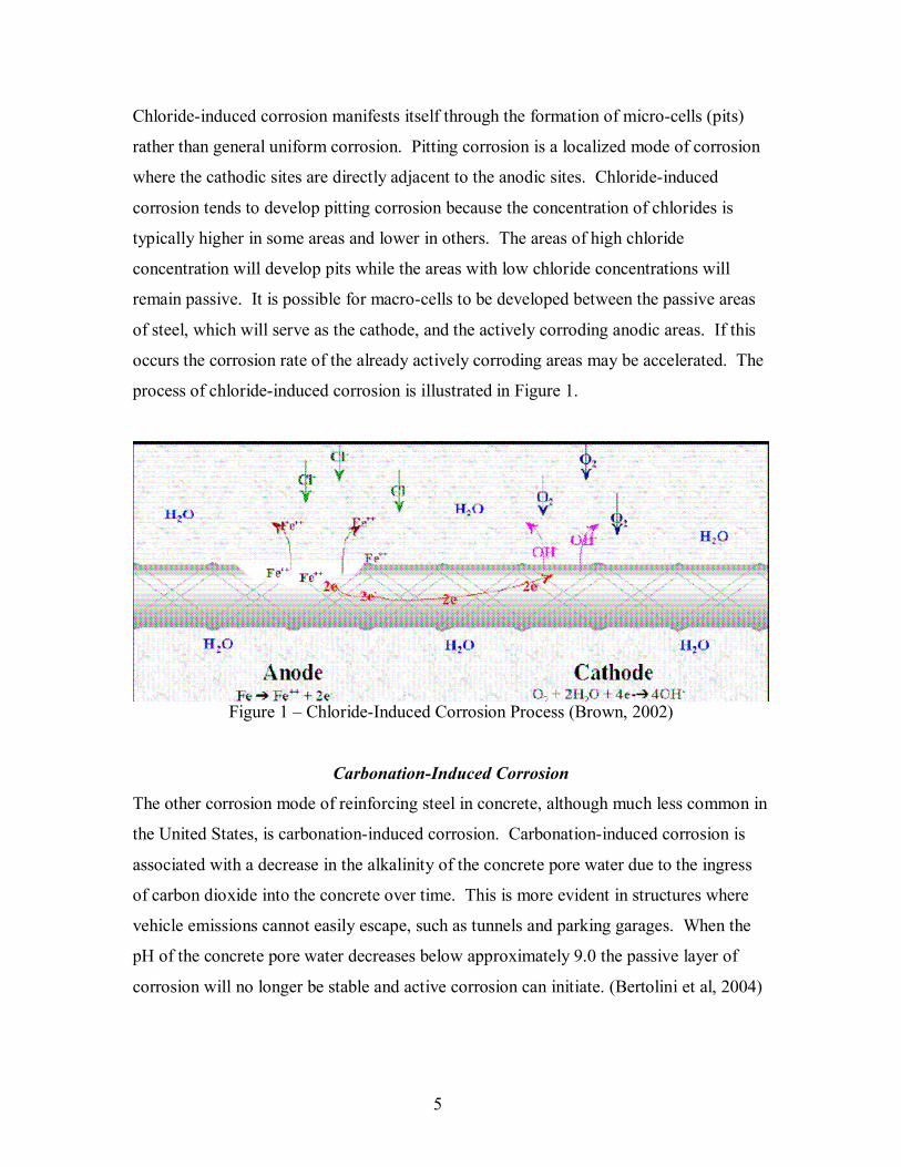
Chloride-induced corrosion manifests itself through the formation of micro-cells (pits)

rather than general uniform corrosion. Pitting corrosion is a localized mode of corrosion

where the cathodic sites are directly adjacent to the anodic sites. Chloride-induced

corrosion tends to develop pitting corrosion because the concentration of chlorides is

typically higher in some areas and lower in others. The areas of high chloride

concentration will develop pits while the areas with low chloride concentrations will

remain passive. It is possible for macro-cells to be developed between the passive areas

of steel, which will serve as the cathode, and the actively corroding anodic areas. If this

occurs the corrosion rate of the already actively corroding areas may be accelerated. The

process of chloride-induced corrosion is illustrated in Figure 1.

Figure 1 � Chloride-Induced Corrosion Process (Brown, 2002)

Carbonation-Induced Corrosion

The other corrosion mode of reinforcing steel in concrete, although much less common in

the United States, is carbonation-induced corrosion. Carbonation-induced corrosion is

associated with a decrease in the alkalinity of the concrete pore water due to the ingress

of carbon dioxide into the concrete over time. This is more evident in structures where

vehicle emissions cannot easily escape, such as tunnels and parking garages. When the

pH of the concrete pore water decreases below approximately 9.0 the passive layer of

corrosion will no longer be stable and active corrosion can initiate. (Bertolini et al, 2004)

6

The pH of the concrete pore water is lowered by the reaction of carbon dioxide with

water and calcium hydroxide. The carbon dioxide initially reacts with water to form

carbonic acid, which then reacts with calcium hydroxide to form calcium carbonate and

water. This reaction process is presented below.

3222 COHOHCO →+

( ) OHCaCOOHCaCOH 23232 2+→+

As more and more of the calcium hydroxide, which is highly alkaline, is consumed by the

reaction, the pH of the concrete pore water becomes lower resulting in the destabilization

of the passive layer. It has been shown that the progression of carbonation can be

modeled as a diffusion process with the rate of diffusion being dependent upon concrete

properties. The concrete factors that affect the carbonation corrosion process to the

greatest degree are: concrete cover depth, cement alkali content, and concrete density.

(Broomfield, 1997)

Carbonation-induced corrosion will typically be reflected as general corrosion over larger

areas of steel as compared to chloride-induced corrosion, which tends to be localized.

Corrosion of Bare Steel in Concrete

The corrosion of bare steel in concrete as related to chloride ingress initiates as described

previously. Corrosion will initiate at a location where the chloride concentration has

reached a critical concentration. Chloride concentrations can vary widely across a deck,

but it is generally observed that the areas of the bridge deck with the lowest cover will

initiate corrosion first. There are many other factors that play a role in where corrosion

will actually intiate and some of those will be discussed in further detail later in this

chapter.

Corrosion of Epoxy-Coated Steel (ECR) in Concrete

Contrary to bare steel ECR will not necessarily initiate corrosion in the areas of the

lowest cover depth. During the fabrication process the steel reinforcing bar is not

7

uniformly coated and small pinholes in the coating, referred to as holidays, may be

present in the finished product. In addition to this, ECR bars are often damaged while in

transit or during construction. These exposed areas are susceptible to chloride-induced

corrosion that will initiate in the same fashion as does bare steel. Because of this the

initiation of corrosion for ECR is less dependent upon cover depth and more dependent

upon the condition of the coating.

Once corrosion has initiated on an ECR bar the corrosion rate will be affected by the

coating as well. The coating acts as a physical barrier to chlorides, oxygen, and water as

well as an electrical barrier. The coating is intended to electrically isolate anodic areas

from cathodic areas. The distance between the anodic areas and cathodic areas is

dependent upon the distance between damaged coating areas on the bar. As this distance

increases the resistance evident in the corrosion cell also increases, which results in a

decreased corrosion rate.

The effectiveness of the epoxy coating in reducing the corrosion rate has been a source of

debate. One area of controversy is whether or not corrosion is able to propagate

underneath the coating. This is largely dependent upon the strength of the bond between

the coating and the bar. One study reports that adhesion loss was evident in bridge decks

as young as 4 years and suggests that �ECR will not provide any or little additional

service life for concrete bridge decks in comparison to black steel�. (Pyc, 1998)

Chloride Threshold Concentrations

As has been established that the concentration of chlorides at the depth of the

reinforcement must reach a threshold value in order for corrosion to initiate and sustain a

significant corrosion rate. It is also known that there is no single value that is appropriate

for use as the threshold concentration. Threshold values can vary widely between bridge

decks as well as within a single bridge deck. This is due to the many factors that affect

corrosion initiation. Several major factors that have been identified are �the

concentration of hydroxyl ions in the pore solution, the potential of the steel, and the

presence of voids at the steel/concrete interface.� (Bertolini et al., 2004) Other factors

8

that are known to affect corrosion threshold concentrations are: cement composition,

moisture content, w/c ratio, and temperature. These factors influence the chloride binding

capacity of the cement paste, the capability for corrosion to initiate based upon the

electrochemical potential of the steel, the ability for localized corrosion (pitting) to form,

and the passive layers� capacity to re-establish itself.

The proper way to report chloride threshold levels and chloride concentrations has been a

point of contention among researchers for many years. The most common methods used

to specify concentrations are: % chloride by weight of cement, weight per unit concrete,

and chloride to hydroxyl ratio. It has been reported that the chloride/hydroxyl ratio must

reach a specified level in order for corrosion to initiate. (Page et al., 1986; Lambert et al.,

1991) This may be true, however, there is still a wide range of reported values and

hydroxyl concentrations are difficult to obtain. A review of the reported values

concluded that �chloride threshold levels are best presented as total chloride contents

expressed relative to the weight of cement.� (Glass and Buenfeld, 1997)

The decision to report the free chloride concentration or the total chloride concentration

is another area of debate. The free chloride concentration is taken to be the water-soluble

concentration and the total concentration is taken to be the acid-soluble concentration.

The difference between the two is the bound chloride concentration. It has been argued

that bound chlorides are not available to initiate or propagate corrosion, however, it has

been shown that as corrosion propagates bound chlorides can be liberated and may

become available to continue the corrosion reaction. Due to the fact that the extent and

mechanism of the liberation of bound chlorides is not fully understood the acid-soluble

chloride concentration less the background chloride concentration will be utilized in this

study. Additionally, the concentration of chlorides per unit of concrete will be the

convention used in this study, as actual cement contents for the bridge decks sampled are

not known and do not vary significantly in Virginia where a minimum cement content

and maximum w/c are specified.

9

Chloride threshold levels also vary depending upon the type of reinforcement present

within the concrete. Alternative reinforcements such as galvanized steel and stainless

steel have much higher threshold levels. Specific ranges and statistical distributions for

chloride threshold values for reinforcement types will be presented in the Method of

Analysis section.

Time to Corrosion-Induced Cracking of Cover Concrete

The corrosion rate of steel in concrete is affected by several factors among which are: the

permeability of the concrete, moisture content of the concrete, temperature, and the

availability of oxygen. The time required for corrosion to propagate to a level where the

concrete will be damaged will vary depending upon the local climate. For example a

region with a dry climate will have a significantly longer propagation time than a region

with a tropical climate due to the lack of moisture in the concrete. For bridge decks in

Virginia it is reasonable to assume a single value for the propagation time, as the climate

does not vary significantly within the state and also because the propagation time is small

relative to the time required to initiate corrosion. A study on the corrosion of reinforcing

steel in the U.S. estimates the propagation time to be between 2 and 5 years for bare steel.

(Weyers et al, 1992) Some increase in propagation time is expected for alternative

reinforcements such as epoxy-coated reinforcement (ECR) and stainless steel

reinforcement.

ECR, the most common alternative reinforcement, provides additional propagation time

by inhibiting the formation of corrosion macrocells. The additional propagation time for

ECR has been estimated to be between 2.7 and 5.7 years. (Weyers et al., 2006) Several

corrosion cracking models will be presented later in the literature review and time to

cracking estimates will be made based upon current construction specifications and

expected corrosion rates for Virginia bridge decks.

Deck Protection, Repair, and Rehabilitation Methods

It has long been known that chlorides from deicing salts are the primary cause of

reinforcement corrosion in bridge decks in the Northern climates of the United States.

10

VDOT, just as nearly all other state agencies, has taken steps to prevent or delay the onset

of chloride-induced corrosion. VDOT has increased cover-depth requirements and

implemented the use of low permeable concretes as well as specified the use of ECR. It

is known that by increasing the concrete cover-depths and using low permeable concretes

the time required for chlorides to penetrate to the depth of reinforcing steel will be

significantly increased. This in turn will delay the onset of corrosion and prolong the

service life of Virginia bridge decks. This section addresses the deck protection, repair,

and rehabilitation methods that are currently available and in use in the U.S. Additional

methods that are under investigation will also be discussed, but not addressed in the

service life and life cycle cost determinations.

Deck Protection Methods

Deck protection methods include those methods that are used to reduce the rate of the

diffusion of chlorides into the concrete, extend the corrosion propagation period, or

prevent active corrosion from initiating.

Deck Sealers

The first protection method that will be discussed is the use of deck sealers. Deck sealers

can either be solvent or water based liquids that are applied to the deck surface creating a

finite impermeable layer, which prevents chloride-laden water from penetrating the

concrete structure. Currently, �only penetrating sealers, silanes and siloxanes (or

combinations), are recommended for deck surfaces. Other sealer types have an

inadequate depth of penetration and quickly wear when exposed to traffic abrasion.�

(Weyers, R.E. et al, 1993) Deck sealers while preventing water from entering the

concrete structure will allow water vapor to escape. This allows for the concrete deck to

dry out, which increases the resistance in the corrosion cell by limiting the electrolyte

(the concrete pore water).

There are, however, limitations to the use of deck sealers. The effectiveness of a sealer is

dependent on the permeability of the original concrete, which cannot always be estimated

due to variability in construction practices. Additionally, it is possible to achieve similar

11

reductions in concrete permeability by reducing the w/c ratio of the concrete and through

the addition of pozzolanic materials to the concrete mixture.

Cathodic Prevention

Cathodic prevention is a technique used to prevent active corrosion from initiating.

Cathodic prevention is the process by which passive reinforcement is cathodically

polarized to increase its potential by applying a low current. Increasing the electrical

potential of the steel will elevate the critical chloride threshold to a point that will in

theory never be reached during the service life of the bridge deck. Another type of

cathodic prevention is the introduction of a sacrificial anode into the deck, typically zinc.

The zinc being a less noble metal will act as the anode, therefore making the steel

reinforcement the cathode. The benefit to having the zinc corrode in place of the steel is

that the zinc corrosion process is less expansive and the corrosion products are able to

diffuse into the surrounding concrete matrix without causing damage to the structure.

The problems with cathodic prevention techniques are that they are expensive, require

constant maintenance, and if the current is interrupted active corrosion can initiate

immediately.

Currently, cathodic prevention systems are only being used for rare cases in the United

States. They are primarily used in coastal structures that are exposed to very high

chloride concentrations or in other specialized cases where corrosion is expected to be

severe or structurally problematic. Implementing a cathodic prevention system is

essentially an admission that the structure is not designed for long-term durability.

Perhaps other corrosion prevention methods should be considered to ensure that

corrosion will not initiate under field conditions.

Stainless Steel (SS) Reinforcement

SS reinforcement is a possible alternative to standard carbon bare steel because it has a

much higher chloride threshold than carbon steel reflecting corrosion rates �at least 50

times lower than that of black steel in chloride contaminated concrete.� (Gu, P. et al,

1996) Clemena reports threshold values for stainless steel of at least 10.4 times greater

12

than carbon steel. (2003) This elevated chloride threshold will never be reached for

nearly all bridge deck applications. To be considered stainless steel the steel must be

composed of at least 10.5% chromium. Additional elements such as nickel and

molybdenum are also added to improve the corrosion resistance and mechanical

properties of the steel. SS is divided into four categories based upon its microstructure:

-- Ferritic

-- Austenitic

-- Martensitic and

-- Austenitic � Ferritic (Duplex)

Currently only austenitic and duplex SS are used as concrete reinforcement as the

mechanical properties of the other types are not comparable to carbon steel. However, a

12% ferritic SS is being considered for use. (Bertolini et al, 2004)

The additional corrosion resistance of SS is due to the formation of a passive layer of

chromium oxide at the surface of the reinforcing bar. This passive layer has a critical

chloride concentration that is much higher than that of carbon steel.

The benefits of using SS over other alternative reinforcements are that the corrosion

resistance is substantially greater and the additional corrosion resistance is a bulk material

property. This means that if the reinforcing bars are damaged during construction, the

corrosion resistance of the reinforcement will remain constant unlike epoxy-coated and

galvanized reinforcement where if the coating is damaged the additional corrosion

resistance may be compromised.

Based on the substantial increase in corrosion resistance for SS reinforcement it would

appear that it would be in wide use, however, using SS may be cost prohibitive for some

bridge deck applications. The initial cost of SS is 6-10 times that of carbon steel, so it

may be cost effective only for bridges where very long service lives must be guaranteed

due to the adverse affects associated with bridge closures or in marine environments

where chloride concentrations can be very high. For example, a bridge with very high

13

traffic flow may require a service life of 100+ years because a closure could result in

substantial economic loss to the surrounding area. As a means to reduce the costs of

incorporating SS into bridge decks, the SS may be used only in the top mat of

reinforcement, where chloride contents are higher. Using SS in the top mat and carbon

steel in the bottom mat, there is a potential for galvanic corrosion to take place.

However, a recent study has shown that �no significant risk of galvanic corrosion exists

when carbon steel and stainless steel are electrically coupled in reinforced concrete

structures�. (Abreu, C.M., et al, 2002)

Another method to reduce the costs associated with using SS was introduced in the U.S.

in 1998. That method was the use of stainless steel clad (SSC) reinforcing bars. SSC

bars are manufactured by forming a tube of stainless steel and then packing it with carbon

steel shavings. The tube is then heated to form a composite material. The purpose of

using SSC bars is to reduce the cost of the reinforcement by using carbon steel cores

while maintaining the excellent corrosion properties of the SS bars. The estimated cost

for SSC bars is approximately $1.00/lb ($2.21/kg) compared to $3.00/lb ($6.62/kg) for

solid SS reinforcing bars. It is hoped that SSC bars will provide the desired service life

of 100 years and be cost effective. A recent study conducted by the Virginia

Transportation Research Council (VTRC) concluded that �stainless steel-clad bars can be

used as direct substitutes for either uncoated black steel or epoxy-coated bars for

effective, corrosion-resistant reinforcement of concrete bridge decks� and recommends

that �stainless steel-clad bars be considered an option for reinforcing new concrete

bridges�. (Clemena, Kukreja, and Napier, 2003) However, it has also been reported that

corrosion at cladding defects and cut ends may be a problem. (Cui and Sagues, 2001 and

2003) Currently there is insufficient data to make any final conclusions on the corrosion

resistance of SSC reinforcement. It is clear that further research is required for this

reinforcement alternative, but initial results are promising. Additionally, the mechanical

properties of one SSC reinforcement have been shown to meet ASTM standards for both

tensile and bond strength. (Stainless UK)

14

Galvanized Steel (GS) Reinforcement

GS reinforcement is another alternative reinforcement that has been employed to increase

the service life of bridge decks. Steel is galvanized using the hot-dip-galvanizing process

in which steel is dipped into molten zinc at a temperature between 435 � 454oC. The zinc

reacts with the steel and oxygen forming a protective layer of zinc oxide. (American

Galvanizers Association, 2006) The thickness of the zinc coating is generally between

100 and 150 µm (.0039 � 0059 in.). The threshold chloride concentration values for GS

reinforcement are at least 2.5 times greater than that of carbon steel, which results in a

time to corrosion initiation 4-5 times longer. The increase in threshold chloride

concentration can be attributed to the fact that galvanized steel will stay passivated in

concrete to pHs as low as 9.5 in comparison to bare steel, which depassivates at a pH of

approximately 11.5. (Yeomans, 2004)

The mechanical properties of GS are comparable to carbon steel and the bond strength

between the GS and concrete is also sufficient.

There are several limitations of GS reinforcement associated with its implementation.

The first limitation is that if the zinc oxide coating is damaged during construction

exposing the carbon steel, the exposed steel may corrode just as normal carbon steel

would. However, it has been shown that the zinc layer surrounding damaged areas will

corrode sacrificially to protect the base carbon steel. The cost of GS is also

approximately 2.5 times that of carbon steel. (Bertolini et al, 2004) It is also important to

note that in concrete with low chloride concentrations carbon steel will have a lower

corrosion rate than GS, but in concrete with moderate chloride concentrations GS will

increase the service life of the bridge deck. Additionally, GS reinforcement is not a

viable option for bridge decks that will have high chloride concentrations being that if the

chloride threshold of the GS is surpassed quickly, the sacrificial benefits of the zinc

coating may only extend the corrosion propagation period of the reinforcing steel by

approximately 5 years. (Bautista and Gonzalez, 1996) It should be noted, however, that

the corrosion products of galvanized rebar are much less voluminous than those resulting

from the corrosion of carbon steel (increase in volume of 150% as compared to 250%).

15

Additionally, it has been shown that the GS corrosion products are friable and that they

�migrate away from reinforcement surface and fill cracks and voids in the cover

concrete�. (Yeomans, 1998) This not only relieves stresses at the reinforcement, but also

densifies the concrete. The effects are that the concrete is much less likely to crack and

the diffusion of chlorides into the concrete is inhibited, both of which will increase the

service life of a bridge deck.

Epoxy-Coated Reinforcement (ECR)

ECR became widely used in the 1980�s as a corrosion prevention method due to the

relatively small additional expense in comparison with a substantial expected increase in

service life. Many state agencies have reported good performance of ECR in bridge

decks, but there have also been instances where substantial corrosion has been evident in

as little as 5 years after construction. (Sagüés and Powers, 1997) It is believed that ECR

protects against corrosion by inhibiting the penetration of oxygen, water, and chlorides

from contacting the steel surface. The epoxy coating may also restrict the ability for a

corroding bar to develop macro-cells by limiting the amount of exposed bare steel that

can act as a cathode. ECR is fabricated using a fusion-bonding method consisting of four

primary steps: 1) Bar surface preparation, 2) Heating of the bar, 3) Powder coating the

bar, and 4) The curing and quenching of the bar. As the epoxy powder comes into

contact with the heated bar it melts and covers the surface. The heat also initiates a cross-

linking reaction that provides the epoxy coating with its� necessary physical and

mechanical properties. (CRSI, 2006)

The epoxy coating adds approximately $0.15/lb ($0.33/kg) to the cost of the

reinforcement, which is a minute amount of the total cost of the structure. However, a

study of ECR bridge decks in Virginia concluded that the increase in service life for ECR

bridge decks over bare steel decks may only be 5 years and that the �service life

extension provided by ECR is not a cost-effective corrosion protection method for bridge

decks in Virginia�. (Brown and Weyers, 2003) The inability of ECR to provide a

substantial increase in service life can be attributed to several problems. The problems

associated with ECR include coating holidays developed during the fabrication process,

16

potential for coating damage during transportation and construction, and debonding of the

coating from the steel surface in moist concrete.

MMFX-2 Reinforcement

MMFX-2 is a relatively new reinforcement alternative. It is a proprietary micro-

composite steel that contains chromium, which provides similar corrosion resistance to

stainless steel. The resistance to corrosion of MMFX-2 is not as great as that of stainless

steel, however the mechanical properties are far superior and the cost is significantly less.

The improved mechanical properties of MMFX-2 steel may not significantly reduce the

total amount of reinforcement required for bridge decks as the required amount of

reinforcing steel is often controlled by temperature and shrinkage spacing requirements.

A recent study by VTRC recommends that MMFX-2 be considered for use in bridge

decks as it �has shown promise as a cost-effective countermeasure for corrosion.�

(Clemena, 2003) Clemena reports that the chloride threshold value for MMFX-2 is in the

range of 4.7-5.9 times that of A615 carbon steel. Another study conducted by the South

Dakota Department of Transportation suggests that the threshold chloride concentration

for MMFX-2 is 3.5 times higher than that of carbon steel and that the corrosion rate once

corrosion has initiated can be as much as 2/3 lower. (Darwin et al, 2003) The increased

chloride threshold for MMFX-2 has also been confirmed by research conducted by Trejo

at the University of Texas A & M who reports threshold values of 7.7 pcy (4.6 kg/m3) for

MMFX-2 as compared to 0.9 pcy (0.5 kg/m3) for carbon steel. (Trejo, 2002)

Corrosion Inhibitors (CI)

Various chemical admixtures referred to as corrosion inhibitors have been used to delay

the onset of corrosion or to slow the corrosion rate of steel in concrete. CIs associated

with preventing pitting corrosion can act: �a) by a competitive surface adsorption process

of inhibitor and chloride ions b) by increasing and buffering of the pH in the local (pit)

environment, and c) by competitive migration of inhibitor and chloride ions into the pit

(so that the low pH and high chloride contents necessary to sustain pit growth cannot

17

develop).� (Bertolini et al, 2004) These different CIs can target the anodic reaction site,

the cathodic reaction site, or both the anodic and cathodic sites.

The effectiveness of CI�s that target the anodic reaction site depends largely upon using

the correct dosage. If the CI concentration is too low the corrosion rate of the steel may

actually be increased. This is because anodic CI�s are designed to reduce the area of the

anodic reaction. Therefore, if some of the anodic area is removed the remaining anodic

area will have a much higher cathode to anode ratio, which will in turn increase the rate

of corrosion for that area. To determine the correct dosage it is necessary to accurately

predict the level of chlorides that will be present within the concrete in the future. Based

on the estimated chloride content, the dosage level can be calculated with a recommended

CI to chloride ratio of 0.6. (Elsener, 2001)

Cathodic site CI�s will reduce the corrosion rate of steel regardless of the dosage level.

This is because the anodic area will remain the same, so any reduction in the cathodic

area will reduce the cathode to anode ratio, which will result in a lower corrosion rate.

There are two methods of application for CI�s: addition to the concrete mixture and

surface application. CI�s are most commonly added to the concrete mixture during

construction to ensure that there will be a sufficient concentration of the inhibitor at the

depth of the reinforcement. Surface-applied CI�s are generally used to slow the corrosion

rate of reinforced concrete structures that are already reflecting some corrosion.

However, the effectiveness of surface applied CI�s is largely dependent upon the

properties of the concrete. If the concrete has a low permeability the CI will not diffuse

through the concrete and reach the depth of the reinforcement and no benefit may be

realized. A report conducted by VTRC found that two surface applied corrosion

inhibitors did not penetrate to the depth of the rebar. (Sharp, 2004) For this reason

surface applied CI�s are rarely used.

18

The use of CI�s in bridge deck patches and overlays has also been investigated by VTRC,

but it was concluded that no �benefit from the use of corrosion inhibiting admixtures�

was evident. (Sprinkel, 2003)

Problems associated with the use of CI�s are: accuracy in determining appropriate

dosage rates, leaching out of CI early on in the life of the structure, and the inability of

surface applied inhibitors to penetrate to the reinforcement depth.

Improved Concrete Properties

In addition to the methods listed above one of the relatively easiest and effective methods

used to delay the onset or prevent the corrosion of reinforcement in concrete is to

improve the properties of the concrete. It is known that the characteristic of concrete that

affects the chloride concentration at the reinforcement depth the most is the permeability

of the concrete. The most common means of reducing the permeability of concrete is by

reducing the w/c ratio of the concrete mixture. In Virginia the w/c ratio for concrete used

in bridge decks has been reduced to 0.45 from 0.47. Additionally, mineral admixtures,

commonly referred to as pozzolans, can be introduced into the concrete mixture to further

reduce the permeability. The most frequently used pozzolans are fly ash (FA), and silica

fume (SF). Pozzolans reduce the permeability of concrete by reacting with free calcium

hydroxides present in the pore water to form cement products, which fill the concrete

pore space. Ground granulated blast furnace slag (GGBFS), used in conjunction with

Portland cement will also reduce the permeability of concrete.

VDOT specifies that low permeable concrete (LPC) be used for bridge deck applications.

However, the effect of LPC on the service life of bridge decks is unclear. The reason for

this is that LPC and ECR as well as an increase in the concrete clear cover depth were all

implemented at approximately the same time. Therefore, the resulting increase in service

life cannot be attributed to any one specification change. It is necessary to investigate the

effect of LPC and an increased cover depth on bridge deck service life in order to

determine if ECR is a major contributing factor.

19

Deck Repair Methods

Repair methods are used to temporarily extend the service life of a bridge deck without

the expense of a major rehabilitation. Deck repairs can restore the deck to an acceptable

level of functionality, but they do nothing with regards to addressing the cause of

deterioration. At some point in the future a repaired deck will require major

rehabilitation or replacement and the cause of deterioration must be dealt with at that

time. The repair methods that will be discussed are patching and bridge deck overlays.

Patching

Deck patching is the primary method that is used to repair areas of deck deterioration.

Deterioration is typically due to corrosion induced spalling and delaminations. Any

degradation caused by the corrosion of the reinforcing steel will extend at least to the top

mat of reinforcement and possibly to the bottom mat as well. Patching can either be

partial-depth or full-depth depending upon the extent of the deterioration. Partial-depth

repairs require that a minimum clearance of 0.75 in (19.05 mm). below the top mat of

reinforcing steel be provided, but the total repair depth should not exceed half the

thickness of the deck. If full-depth patches are required, the concrete will be removed in

its entirety for the area of the deck that is to be patched. (Weyers, R.E. et al, 1993)

The materials that are used for deck patching are Portland Cement Concrete (PCC),

hydraulic concretes and mortars, and polymer modified concretes and mortars.

Deck patches provide only a short-term solution to deterioration problems within a bridge

deck. For deterioration related to corrosion, the underlying problem is not addressed and

the reinforcement will continue to corrode in the surrounding deck area. The corrosion

rate of the surrounding steel may actually increase as the patched area will contain very

low chloride concentrations and will therefore become cathodic, which will in turn drive

the adjacent actively corroding anodic sites. For this reason current research is

investigating the possibility of introducing small cubes of zinc into patched areas that will

act as sacrificial anodes, which will prevent the surrounding steel from continuing to

corrode for a short period of time. However, after the zinc is consumed the

20

reinforcement in the deck will once more become anodic and corrosion will progress just

as before.

Deck Overlays

Deck overlays can be used either as a repair method or a rehabilitation method. When

used as a repair method, overlays are placed on the surface of sound concrete that has not

yet begun to deteriorate as a consequence of reinforcement corrosion. The reason

overlays are placed is to decrease the permeability of the concrete and increase the cover-

depth of the concrete, which in turn increases the distance that chloride ions must diffuse

to reach the depth of the reinforcement. Overlays can be either latex modified concrete

(LMC), low-slump dense concrete (LSDC), polymer concrete (epoxy), micro-silica

concrete (MSC), or hot-mix asphalt concrete and membrane (HMAM) systems.

Depending on the overlay type the service life of a bridge deck may be extended by over

25 years. (Weyers, R.E. et al, 1993) However, the increase in the dead load on the bridge

will decrease the live load carrying capacity of the bridge. Additionally, if an overlay is

placed on a bridge deck that already contains a critical level of chlorides present in the

concrete there will only be a small extension to the service life of the deck due to a

reduction in the moisture content of the underlying concrete deck.

Problems associated with bridge deck overlays are: debonding of the overlay from the

deck, shrinkage cracking of the overlay, and determining the appropriate time to install

an overlay on a deck. When specified as a repair or corrosion prevention method, the

most commonly used overlay type in Virginia is multiple layer polymer concrete, which

will significantly reduce the permeability of the concrete and improve skid resistance and

surface apperance. Additionally, the time required for installation is significantly less

than for other overlay alternatives.

Deck Rehabilitation Methods

Deck rehabilitation methods are used to restore a bridge deck to an acceptable level of

performance and to address the cause of deterioration. Deck overlays and cathodic

protection will be discussed in this section.

21

Deck Overlays

Deck overlays when used as a repair method are placed over sound concrete. When a

deck is already reflecting significant damage, those areas must be repaired before the

deck is overlaid and this is considered to be rehabilitation. Those deck areas that are

experiencing active corrosion, are deteriorated, or have a critical concentration of

chlorides must be removed and replaced prior to the installation of the overlay. This

addresses the cause of the deterioration, that being corrosion of the reinforcement. Future

corrosion will be delayed due to the increase in the cover depth and the decrease in

permeability of the deck. It has been estimated that deck overlays that are used to

rehabilitate decks may provide up to 70 years of additional service life. (Weyers, R.E. et

al, 1993)

Cathodic Protection

Cathodic protection differs from cathodic prevention in that it is used on structures that

are already experiencing corrosion. For cathodic protection, titanium anodes are placed

into the concrete and a current is introduced to reduce the corrosion potential to a level

where corrosion is slowed or stopped. If the current is strong enough, the reinforcing

steel will repassivate and corrosion will stop. Cathodic protection has proven to be an

effective means of rehabilitating concrete structures with high chloride concentrations

without having to conduct major rehabilitation. The problems associated with using

cathodic protection are that incorporating the systems tends to be costly and constant

monitoring of the systems is required.

Chloride Diffusion Models

As mentioned previously, the corrosion of bridge deck reinforcing steel is primarily

associated with the diffusion of chlorides into the concrete. For that reason the service

life estimation methods discussed will only address chloride-induced corrosion and not

carbonation-induced corrosion.

22

Chloride diffusion models can be divided into two categories: Fickian and Finite

Element. Fickian diffusion models, the most commonly used models, assume that

chlorides diffuse into the concrete according to Fick�s Second Law of Diffusion. Finite

element diffusion models are based upon averaging the microscopic transport equations

for moisture and ionic diffusion over a representative volume element. Finite element

models are also capable of accounting for the effects of localized chemical reactions and

chemical damage.

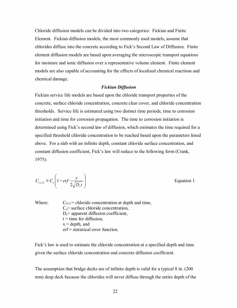
Fickian Diffusion

Fickian service life models are based upon the chloride transport properties of the

concrete, surface chloride concentration, concrete clear cover, and chloride concentration

thresholds. Service life is estimated using two distinct time periods, time to corrosion

initiation and time for corrosion propagation. The time to corrosion initiation is

determined using Fick�s second law of diffusion, which estimates the time required for a

specified threshold chloride concentration to be reached based upon the parameters listed

above. For a slab with an infinite depth, constant chloride surface concentration, and

constant diffusion coefficient, Fick�s law will reduce to the following form (Crank,

1975):

−=

tDxerfCC

cotx 2

1),( Equation 1

Where: C(x,t) = chloride concentration at depth and time,

Co= surface chloride concentration, Dc= apparent diffusion coefficient, t = time for diffusion, x = depth, and erf = statistical error function.

Fick�s law is used to estimate the chloride concentration at a specified depth and time

given the surface chloride concentration and concrete diffusion coefficient.

The assumption that bridge decks are of infinite depth is valid for a typical 8 in. (200

mm) deep deck because the chlorides will never diffuse through the entire depth of the

23

deck over the life span of the structure. To use Equation 1 shown above the diffusion

coefficient (Dc) and the surface chloride concentration (Co) must be taken as constants

over time, however, it is known that both Dc and Co are time-dependent parameters. The

effects of their time-dependent nature and the methods that are used to account for them

are discussed in the following two sections.

Effect of Time-Dependent Diffusion Coefficients

As mentioned previously, the diffusion coefficient used to estimate the service life of a

bridge deck is a time-dependent parameter. Work by Bamforth (1999) and Mangat and

Molloy (1994) clearly indicate that the rate of chloride ingress into concrete reduces with

time. The rate of reduction will differ between bridge decks depending upon the

composition of the concrete as well as environmental conditions.

The most commonly cited reason for a reduction in Dc is continued hydration of the

cement. Pozzolanic reactions within the concrete m atrix will also result in a reduction in

Dc. Additionally, it has been speculated that the presence of insoluble salts at the surface

of the concrete will slow the ingress of chlorides by acting as a physical barrier. All of

the mechanisms listed manifest themselves within concrete differently, however, they all

result in a decrease in Dc by constricting the capillary pore system. While the exact

chemical and physical phenomena that precipitate changes in Dc are not fully understood,

they can be reasonably modeled from empirical data.

It has been shown that the initial Dc for a concrete mixture is relatively high, but will

reduce rapidly reaching a near steady state in 5-10 years. The magnitude and rate of

reduction are dependent primarily upon the w/c ratio of the concrete, amount and type of

pozzolan present, and the rate of hydration. The most effective method available to

reduce Dc is the addition of pozzolan to the concrete mixture. Pozzolans act as secondary

cementitious materials, which react to form hydration products after the initial hydration

of the cement. The pozzolanic hydration products fill the capillary pore space resulting

in a less permeable concrete.

24

The effect of the time-dependency of Dc will vary subject to the magnitude of the

reduction and the time of first exposure to chlorides. Clearly if a bridge deck is exposed

to deicing salts at a very young age (<3 months), the effect on service life estimations

will be much greater than if the deck is first exposed at an age greater than 6 months. In

order to accurately model the effective diffusion coefficient it is necessary to know the

age at which the deck will be first exposed. This, of course, is difficult to predict and

impossible to know for bridges that are already in place. A more reasonable approach to

estimating the service life for bridges that are in place is to use the apparent diffusion

coefficient (Dca) at some specified time, for example, at 10 or 20 years. Several models

are available that can be used to estimate Dca for a given bridge deck and they will be

presented in the Fickian Diffusion Models section.

Effect of Time-Dependent Surface Chloride Concentrations

It is known that the chloride concentration at the surface (Co) of a bridge deck will

increase over a period of time and eventually become relatively constant at some

maximum value. This is evident in data collected by Weyers et al. for 15 bridge decks in

the snow-belt region over a 15-year period. (1994) However, most researchers use a

constant Co to predict the service lives of bridge decks. Kassir and Ghosn completed a

research project that investigated the effect of a time-varying Co and found that in some

cases the difference in predicted service lives can be as much as 100%. (2002) The

influence was modeled by incorporating an exponentially time-varying Co term into the

standard Fickian equation.

While it is true that some cases had differences in predicted services lives of up to 100%,

for a typical Virginia bridge deck the differences are expected to be in the range of 5-

15%. These differences are relatively small when taken in context of a 100-year service

life. Additionally, these calculations do not take into account the effect of a time-

dependent diffusion coefficient, which will counteract the effects of time-dependent Co

values. In order to accurately predict bridge deck service lives using these parameters it

is imperative that the age of the deck be known at the time of first salt application and

also the nature of the time-dependency of the specific concrete mixture. For that reason

25

this research will disregard the effect of time-varying Co values and will only investigate

the effects of time-varying Dc values to select an appropriate time for the measuring of

apparent Dc.

Effect of Pozzolans

A pozzolan is defined as a �siliceous or siliceous and aluminous material, which in itself

possesses little or no cementitious value but will, in finely divided form and in the

presence of moisture, chemically react with calcium hydroxide at ordinary temperatures

to form compounds possessing cementitous properties.� (ASTM) Pozzolans are used as a

partial replacement for cement in a concrete mixture to increase strength and decrease the

permeability of the resultant concrete. The improved properties of concrete containing

pozzolans are attributable to the mechanism in which pozzolans react within the concrete

mixture. Pozzolans react with calcium hydroxide, a by-product of the hydration of

cement present within the concrete pore water, to form additional cementitous materials.

These materials further densify the concrete matrix resulting in higher compressive

strengths and lower permeabilities. Additionally, the reaction consumes much of the

available alkali, which reduces the potential for alkali-aggregate reactivity.

Pozzolans that are currently in use can be either naturally occurring or manufactured.

Some examples of natural pozzolan are volcanic ash, tuff, clays and shales. Typical

manufactured pozzolans are fly ash, microsilica (silica fume), and ground-granulated-

blast-furnace slag (GGBFS). These materials are by-products from coal burning power

plants, silicon metal production, and iron ore reduction, respectively.

The use of pozzolans in concrete not only provides higher quality concrete, but also has

economic and environmental benefits as well. However, care should be taken when

introducing a pozzolan into a concrete mixture as water demand, setting time, and early

age strength can be adversely affected. The effects are due primarily to differences

between the fineness of cement and pozzolan.

26

Pozzolans are currently used in the construction of bridge decks to provide a low

permeable concrete. The reduced permeability of the concrete will slow the ingress of

chlorides into the concrete resulting in the delayed onset of reinforcement corrosion. The

permeability of concrete containing pozzolan will continue to decrease with time just as

does Ordinary Portland Cement concrete, however, it will do so at a faster rate beyond

early ages. It should be noted that in order to obtain the beneficial effects of using

pozzolans, it is necessary to maintain high levels of quality control as increases in the w/c

ratio can negate the positive effects of the pozzolans.

Effect of Chloride Binding

It has been well documented that chlorides can be bound either physically or chemically

to hydration products. (Tang and Nilsson, 1993; Martín-Pérez et al., 2000) As free

chlorides are bound to hydration products the amount of chlorides available to induce

corrosion of the reinforcement is reduced. This last point is somewhat controversial; as it

has been argued that as the free chloride concentration is reduced by the corrosion

reaction the bound chlorides will be liberated and become available to continue the

reaction. Tang and Nilsson (1993) proposed that some chlorides are �irreversibly

combined into hydrated products by chemical reaction, and others can unbind as the free

chloride concentration decreases.� This phenomenon is still not entirely understood and

alterations to available chloride diffusion models based upon chloride binding should be

done so with caution.

Chloride binding is typically modeled by using one of three isotherms (Martín-Pérez et

al., 2000): Linear, Langmuir, or Freundlich. These isotherms are presented below.

Linear isotherm: fb CC α= Equation 2

where: Cb = Concentration of bound chlorides (kg/m3 of concrete)

α = Slope of the line

Cf = Concentration of free chlorides (kg/m3 of pore solution)

27

Langmuir isotherm: f

fb C

CC

βα+

=1

Equation 3

where: α, β = Binding constants that vary depending upon the binder composition

Freundlich isotherm: βα fb CC = Equation 4

The linear isotherm is the most simplistic and most convenient to use, but does not reflect

the non-linear binding properties of the cement paste. It will overestimate the bound

chlorides at high free concentrations and underestimate them at low concentrations.

(Martín-Pérez et al., 2000) Realizing the non-linear nature of the problem some still

believe that a linear isotherm is an adequate representation of the phenomenon. (Sergi et

al., 1992)

Tang and Nilsson (1993) have shown that the Langmuir isotherm best describes the

relationship between the bound chloride and the free chloride for low free-chloride

concentrations (< 0.05 mol/l) and the Freundlich isotherm is better suited for high free-

chloride concentrations (> 0.01 mol/l)

The problem associated with incorporating chloride binding into diffusion models is that

it is necessary to experimentally determine the isotherm chloride binding constants for

every concrete mixture that is to be investigated. This can be a difficult and time-

consuming process and values can vary greatly depending upon the w/c ratio, pozzolan

content, and C3A content of the concrete.

For this project the effects of chloride binding will be neglected. The chloride initiation

concentrations from the literature are based upon total chloride concentrations less a

background concentration. Therefore, in order to relate chloride measurements from this

project to reported values the total chloride concentrations must be used. The background

chloride concentrations to be subtracted out will be determined by analyzing the chloride

concentrations in the concrete below the reinforcing steel. The chlorides found at this

28

depth will be taken to be irreversibly bound either within the cement paste or the

aggregate.

Fickian Diffusion Models

Cady and Weyers (1983)

Cady and Weyers developed a service life model for bridge decks based upon chloride-

induced corrosion of the reinforcing steel. The ingress of chlorides into the concrete is

taken to be primarily the result of Fickian diffusion and moisture flow through

subsidence cracks. For areas of the deck where subsidence cracking is present, corrosion

of the reinforcement is taken to be instantaneous. Chloride ingress in uncracked areas is

estimated using Fick�s 2nd Law of Diffusion as presented earlier.

Empirical data for Co, Cx,t, Dc, and x were used as input to develop service life estimates

for a typical 0.45 w/c, OPC bridge deck. (Page et al, 1981; Goto and Roy, 1981; Clear,

1975; Clear, 1976) Subsidence cracking is dependent upon the cover depth with smaller

cover depths resulting in more cracking. The extent of cracking was estimated using

cover depth data gathered in a previous study and an assumed 2 in. (50 mm) slump.

(Dakhil et al., 1975) Using that data, the initial subsidence cracking for a typical bridge

deck was estimated to be 4.07%. Therefore, 4.07% of a bridge deck is expected to

initiate corrosion upon the first exposure of the deck to chlorides and subsequent

corrosion initiation is estimated by Fickian diffusion.

The modeling was an early attempt at estimating the service lives of bridge decks and is

limited in scope. Service life estimates made using this model assume that subsidence

cracking will occur on all bridge decks to some degree regardless of concrete quality and

that concrete diffusion properties are constant. Additionally, the model is deterministic

and therefore is not capable of modeling the effects of input data variability. Since its�

conception many modifications to this model have been proposed to better estimate

bridge deck service life and are presented below.

29

Mangat and Molloy

Mangat and Molloy (1994) developed a diffusion model that accounts for time-dependent

diffusion. The model approximates the relationship between Dc and time with the

following empirical relationship:

m

ic tDD −= Equation 5

where:

Dc = Effective diffusion coefficient at time t (cm2/s)

Di = Effective diffusion coefficient at time t equal to 1 second

t = Time (s)

m = Empirical coefficient that varies with mixture proportions

In order to estimate Di for a particular concrete mixture a regression analysis must be

performed on empirical data fitted to a log-log plot. Di is then projected based upon that

analysis and m is taken to be equal to the slope of the regression line. It was also found

that m can be estimated if the w/c ratio of the mix is known using the following equation:

6.05.2 −

=

cwm Equation 6

The corresponding closed form solution to the diffusion problem is then:

( )

−

−=−mi

otx

tm

DxerfCC

1),(

12

1 Equation 7

This equation is valid only when the initial diffusion coefficient is taken at t = 1 second

and the age at the time of first exposure to chlorides is also taken to be at t = 1 second.

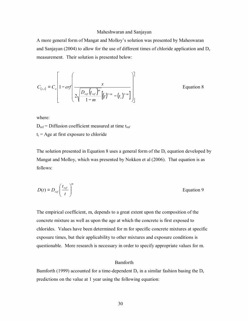
30

Maheshwaran and Sanjayan

A more general form of Mangat and Molloy�s solution was presented by Maheswaran

and Sanjayan (2004) to allow for the use of different times of chloride application and Dc

measurement. Their solution is presented below:

( ) ( ) ( ) ( )[ ]

−−

−=−− m

im

mrefref

otx

ttm

tD

xerfCC11

,

12

1 Equation 8

where:

Dref = Diffusion coefficient measured at time tref

ti = Age at first exposure to chloride

The solution presented in Equation 8 uses a general form of the Dc equation developed by

Mangat and Molloy, which was presented by Nokken et al (2006). That equation is as

follows:

m

refref t

tDtD

=)( Equation 9

The empirical coefficient, m, depends to a great extent upon the composition of the

concrete mixture as well as upon the age at which the concrete is first exposed to

chlorides. Values have been determined for m for specific concrete mixtures at specific

exposure times, but their applicability to other mixtures and exposure conditions is

questionable. More research is necessary in order to specify appropriate values for m.

Bamforth

Bamforth (1999) accounted for a time-dependent Dc in a similar fashion basing the Dc

predictions on the value at 1 year using the following equation:

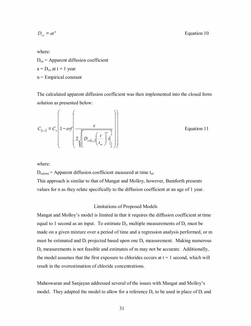
31

nca atD = Equation 10

where:

Dca = Apparent diffusion coefficient

a = Dca at t = 1 year

n = Empirical constant

The calculated apparent diffusion coefficient was then implemented into the closed form

solution as presented below:

( )

( )

−=

tttD

xerfCCn

mtca

otx

m2

1, Equation 11

where:

Dca(tm) = Apparent diffusion coefficient measured at time tm

This approach is similar to that of Mangat and Molloy, however, Bamforth presents

values for n as they relate specifically to the diffusion coefficient at an age of 1 year.

Limitations of Proposed Models

Mangat and Molloy�s model is limited in that it requires the diffusion coefficient at time

equal to 1 second as an input. To estimate Di, multiple measurements of Dc must be

made on a given mixture over a period of time and a regression analysis performed, or m

must be estimated and Di projected based upon one Dc measurement. Making numerous

Dc measurements is not feasible and estimates of m may not be accurate. Additionally,

the model assumes that the first exposure to chlorides occurs at t = 1 second, which will

result in the overestimation of chloride concentrations.

Maheswaran and Sanjayan addressed several of the issues with Mangat and Molloy�s

model. They adapted the model to allow for a reference Dc to be used in place of Di and

32

also accounted for the possibility of first chloride exposure occurring at times other than t

= 1 second. However, estimating an appropriate value for m still remains difficult.

Bamforth�s model uses an apparent Dc (Dca) value, which is an approximation of Dc, a

time-dependent variable. Maheswaran and Sanjayan (2004) demonstrated numerically

that the empirical constant n used in Bamforth�s model is a function of time and cannot

be used to accurately estimate a Dca value.

It is also important to note that the rate at which Dc will reduce is highly dependent upon

mixture proportions. The rate is affected by w/c ratio, pozzolan content, and curing

conditions. It is clear that due to the high variability in mixture proportioning and curing

conditions that estimating appropriate parameters for calculating a time-dependent Dc

remains a difficult task. Therefore, this project will first attempt to model the diffusion of

chlorides using Fick�s second law of diffusion with a constant apparent Dc value

determined from field measurements. The apparent Dc value that is used will be the

value determined at the time of sampling, the apparent Dc�s are to be considered constant

values normalized over the lifespan of the structure.

Finite Element Method (FEM) Modeling of Diffusion

The Finite Element Method is a numerical analysis technique used to approximate the

solution to a set of partial differential equations. It has many applications in engineering

including the analysis of structural, thermal, and fluid systems. In recent years FEM has

also been applied to diffusion problems, specifically the diffusion of chlorides into

concrete.

FE modeling of chloride diffusion is a formidable task due to the inherent complexities of

the diffusion process. The parameters that affect chloride diffusion that can be

incorporated into a FE model include: the ionic fluxes of the various ionic species

present within the concrete pore water, moisture flux, heat transfer, chemical reactions,

and chemical damage.

33

The diffusion of chlorides has been described using simple Fickian behaviour, but it is

known that the rate of chloride diffusion is affected by the prescence of other ionic

species within the pore water. To model the diffusion of chlorides, the fluxes of each

ionic species must be accounted for, as chlorides are charged particles that are affected by

electrical forces including those created by other ions. These forces can result in either

the increasing or decreasing of chloride diffusion.

The exposure conditions of a bridge deck require that changes in moisture and heat

transfer be accounted for, as the moisture content of the concrete and ambient

temperature will change over the course of a year. To model the time-dependent nature

of these parameters, it is necessary to use the Finite Difference Method (FDM). The

FDM is a numerical analysis technique used to approximate the differential equation

rather than its� solution as FEM would. FDM is less robust and is not capable of

handling complex geometries. However, due to the simple geometry of the assumed one-

dimensional diffusion problem and the ease of FDM incorporation, it is commonly used

to model time-dependent parameters.

The use of FEM has also made it possible to model the effects of chemical reactions and

chemical damage. The chemical reactions of concern are those relating to the binding of

chlorides and those that affect the pore structure of the concrete.

While the use of FEM to estimate the diffusion of chlorides into concrete may provide

much more detail and may account for many more parameters than those investigated in

Fickian models, being able to account for the statistical nature of the input parameters

remains a problem. Additionally, the required input data for a FEM model demands a

much higher level of testing on the concrete, which is time consuming and costly.

FEM Diffusion Models

Saetta, Scotta, and Vitaliani (1993)

Saetta et al. developed a numerical procedure based upon the FEM to solve a set of

nonlinear equations that describe the movement of chlorides through partially saturated

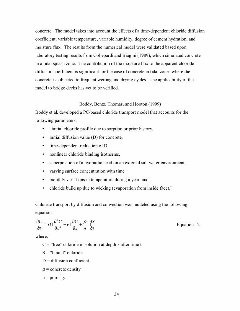
34

concrete. The model takes into account the effects of a time-dependent chloride diffusion

coefficient, variable temperature, variable humidity, degree of cement hydration, and

moisture flux. The results from the numerical model were validated based upon

laboratory testing results from Collepardi and Biagini (1989), which simulated concrete

in a tidal splash zone. The contribution of the moisture flux to the apparent chloride

diffusion coefficient is significant for the case of concrete in tidal zones where the

concrete is subjected to frequent wetting and drying cycles. The applicability of the

model to bridge decks has yet to be verified.

Boddy, Bentz, Thomas, and Hooton (1999)

Boddy et al. developed a PC-based chloride transport model that accounts for the

following parameters:

• �initial chloride profile due to sorption or prior history,

• initial diffusion value (D) for concrete,

• time-dependent reduction of D,

• nonlinear chloride binding isotherms,

• superposition of a hydraulic head on an external salt water environment,

• varying surface concentration with time

• monthly variations in temperature during a year, and

• chloride build up due to wicking (evaporation from inside face).�

Chloride transport by diffusion and convection was modeled using the following

equation:

tS

nxCv

xCD

tC

∂∂⋅+

∂∂⋅−

∂∂⋅=

∂∂ ρ

2

2

Equation 12

where:

C = �free� chloride in solution at depth x after time t

S = �bound� chloride

D = diffusion coefficient

ρ = concrete density

n = porosity

35

v = average linear velocity = dxdh

nk

nAQ ⋅−=

Q = flow rate

A = cross-sectional area

k = hydraulic conductivity

h = hydraulic head

The above equation can be explained simply as the rate of change in chloride

concentration with respect to time is equal to the summation of the effects of chloride

diffusion, convective flow, and chloride binding.

The input parameters that are required by the program are as follows:

• �m, constant dependent on mix proportions, which controls the rate of reduction

of diffusivity,

• T, absolute temperature of exposure for structure,

• Ccrit, threshold concentration or critical chloride level required to initiate corrosion

of steel,

• Dref, diffusion coefficient at some reference time tref and temerature Tref,

• kref, permeability coefficient at some reference time tref,

• Co, surface concentration, and

• depth of cover�

The proposed diffusion model relies on several basic assumptions used to simplify the

diffusion process. The assumption that the concrete is fully saturated is the most notable.

By making this assumption, the model does not incorporate the effect that capillary

absorption has on the transport of chlorides. In addition to this Dc is calculated using

Fick�s law instead of taking into account the influences of opposing ionic fluxes.

Another important aspect to note is that the model is highly sensitive to the input

parameter m. The value for m that is used is selected based upon the concrete mixture

composition. To date, there is not adequate research to determine appropriate values of

36

m for specific mixture proportions with confidence. A sensitivity analysis was conducted

and predicted changes in service lives of up to 550% with only moderate variations in m

were observed. Because of this there is certainly some question as to the ability of this

model to accurately estimate the service lives of concrete structures. Additional testing to

determine the effective diffusion rate and concrete permeability is also required in order

to use this model.

Martín-Pérez, Pantazopoulou, and Thomas (2001)

Their model is an improvement upon the Boddy et al. model presented above in that the

effects of moisture flux are included. Additionally, the model includes the diffusion of

oxygen as a supplementary controlling factor once corrosion has initiated. However, as

was the case in the Boddy model, the influence of ionic electrical coupling is not

accounted for and the model remains deterministic in nature.

The model uses a �numerical formulation of the associated mass transport partial

differential equations� that is �solved in space using a finite element formulation and in

time using a finite difference marching scheme.�

This model has addressed several limitations that were evident in the Boddy model.

However, given the case that a FE model is capable of accurately predicting the time to

diffusion and corrosion for one set of input variables, it is still necessary to account for

the variability in the input data. This is a problem that is not easily handled by FEM due

to the complexity of the calculations required.

Commercially Available Models

STADIUM

STADIUM is a computer-based �numerical model that predicts the mechanisms of ionic

transport in unsaturated cement systems.� (Marchand, 2000) The model incorporates the

effects of ionic diffusion, moisture transport, chemical reactions, and chemical damage.

STADIUM is, to the author�s knowledge, the only diffusion model currently available

that is capable of modeling the electrical coupling between various ionic species as well

37

as the chemical equilibrium reactions between the solid and liquid phases of the concrete

matrix. STADIUM is primarily designed to model ionic flow within cement-based

systems; however, there are other potential applications such as modeling ionic flow

through soils and porous membranes.

The model is based upon determining the transport mechanisms at the microscopic scale

and then averaging them over a Representative Elementary Volume (REV) using the

homogenization technique. The REV must be of sufficient size to adequately model the

pore space as well as the surrounding cement paste and is typically on the order of a few

cubic centimeters in size. (Samson et al, 2005)

STADIUM is currently capable of estimating the electrical coupling between six ionic

species those being: OH-, Na+, K+, S −24O , CA2+, and Cl-. In addition to modeling ionic

electrical coupling, STADIUM incorporates the chemical equilibrium reaction equations

for five different solid phases. Those phases, considered to be the most important, are

Portlandite, Ettringite, Hydrogarnet, Friedel�s salt, and Gypsum.

As might be expected, in order to model these complex equations extensive user input is

required. A list of the necessary input data is presented below:

• Material density

• Paste content

• Diffusion coefficients

• Water diffusivity

• Total porosity

• Capillary porosity

• Initial values of ion concentration, volumetric water content in the pores, and

electrical potential

• Initial amount of solid phases

• Equilibrium constants

• Boundary conditions for ion concentration, volumetric water content in the pores,

and electrical potential

38

• Temperature

To acquire the input data a number of tests and calculations must be conducted including:

determination of the initial composition of the material by evaluating the chemical make-

up of the binder, degree of hydration, and mixture characteristics; determination of the

initial composition of the pore water; determination of the initial total porosity using

standard procedures such as ASTM C 642; calculation of the capillary porosity;

migration tests to determine the diffusion coefficient of the material; and determination of

the water diffusion coefficient by nuclear resonance imaging. (Marchand, 2000)

STADIUM is a robust diffusion model that accounts for many material and

environmental factors that effect the diffusion of various ionic species within a cement

based system. It has potential applications in many fields, however, due to the

complexity of the model and the required user input, implentation for general engineering

applications may pose some difficulty. When evaluating the feasibility of applying this

model to the corrosion of reinforcing steel within a bridge deck the extensive testing

required must be considered. It is also noted that incorporating the statistical nature of

the input variables into this model may prove to be a difficult task.

Life-365 (Thomas and Bentz, 2000)

Life-365 is a computer-based model that was developed for the American Concrete

Institue (ACI). The models� intended use is as a service life estimation and Life Cycle

Cost Analysis (LCCA) tool for engineers for a wide variety of applications. Life-365

estimates the service life for a reinforced concrete structure using a four-step approach.

The four steps are:

1) �Predicting the time to the onset of corrosion, commonly called the initiation

period, ti

2) Predicting the time for corrosion to reach an unacceptable level, commonly called

the propagation time, tp

3) Determining the repair schedule after first repair

39

4) Estimating life-cycle costs based on the initial concrete (and other protection)

costs and future repair costs�

The time to the onset of corrosion is estimated using basic Fickian behaviour as described

previously using a finite difference approach to account for the time-dependency of Dc

and Co. The propagation time is taken as a set value that is selected by the user.

To provide a user-friendly tool Life-365 uses a simplified approach to estimating the

diffusion process. The model assumes that �ionic diffusion is the sole mechanism of

chloride transport� and that the concrete is �completely saturated.� By doing so, the

amount of required input is significantly reduced. The input parameters that are required

by the model are as follows:

• Co � Surface concentration

• D � Diffusion coefficient

• m � Diffusion decay index

• Ct � Chloride threshold

• tp � Propagation period

• Temperature

All of the input parameters can either be user defined or determined by Life-365 based

upon concrete mixture proportions and geographic location. The model is not currently

capable of integrating the variability of the input parameters and can be used only as a

deterministic model. In order to make the program easier to use many assumptions and

simplifications were made. It is recommended that the user take caution when accepting

the default values provided by the program and that actual field data be used whenever

available.

The authors proposed future improvements to the model and they are listed below:

• �Upgrade the propagation period portion of the model, including life-cycle

costing analysis.

40

• Include probabilistic considerations in the model to account for the variability in

input parameters and field construction conditions.

• Include additional corrosion protection products.

• Refine the model as appropriate as additional field verification data becomes

available.� (Thomas and Bentz, 2000)

Corrosion-Induced Cracking of Concrete Cover

As described previously, the dissolution of iron due to corrosion and subsequent

formation of corrosion products (hydrated ferric oxide) results in a volumetric expansion.

As corrosion progresses and more and more corrosion products are formed, stresses are

developed within the concrete structure. Once the tensile strength of the concrete that

surrounds the reinforcement is surpassed it will crack as illustrated in Figure 2. Cracking

of the cover concrete will ultimately result in the spalling or delamination of the deck

surface.

Corrosion-cracking models have been developed to attempt to estimate the time required

for corroding bare steel reinforcement to crack the cover concrete.

Figure 2 � Corrosion-Induced Cracking

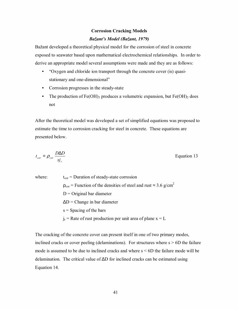
41

Corrosion Cracking Models

Ba�ant�s Model (Ba�ant, 1979)

Ba�ant developed a theoretical physical model for the corrosion of steel in concrete

exposed to seawater based upon mathematical electrochemical relationships. In order to

derive an appropriate model several assumptions were made and they are as follows:

• �Oxygen and chloride ion transport through the concrete cover (is) quasi-

stationary and one-dimensional�

• Corrosion progresses in the steady-state

• The production of Fe(OH)3 produces a volumetric expansion, but Fe(OH)2 does

not

After the theoretical model was developed a set of simplified equations was proposed to

estimate the time to corrosion cracking for steel in concrete. These equations are

presented below.

rcorcor sj

DDt ∆= ρ Equation 13

where: tcor = Duration of steady-state corrosion

ρcor = Function of the densities of steel and rust ≈ 3.6 g/cm2

D = Original bar diameter

∆D = Change in bar diameter

s = Spacing of the bars

jr = Rate of rust production per unit area of plane x = L

The cracking of the concrete cover can present itself in one of two primary modes,

inclined cracks or cover peeling (delaminations). For structures where s > 6D the failure

mode is assumed to be due to inclined cracks and where s < 6D the failure mode will be

delamination. The critical value of ∆D for inclined cracks can be estimated using

Equation 14.

42

ppt DLfD δ'2=∆ Equation 14

where: f�t = Tensile strength of concrete

L = Concrete cover thickness

δpp = Bar hole flexibility

The bar hole flexibility is taken to be the average of the calculated flexibility for a bar in

a thick-wall cylinder and the flexibility for a bar in infinite space. The equations for both

cases are presented below.

Thick-wall cylinder

( )efef

ppo

EsD

ED

2

321 ++= νδ Equation 15

where: ν = Poisson�s ratio

Eef = Effective elsastic modulus = cr

cEΦ+1

Фcr = Creep coefficient of the concrete

Infinite Space

( ) efef

ppEsD

DLLD

ED

2

321 2

21 +

+

++= νδ Equation 16

The equation for the alternative failure mode of delamination is:

ppt DsfD δ

−=∆ 1' Equation 17

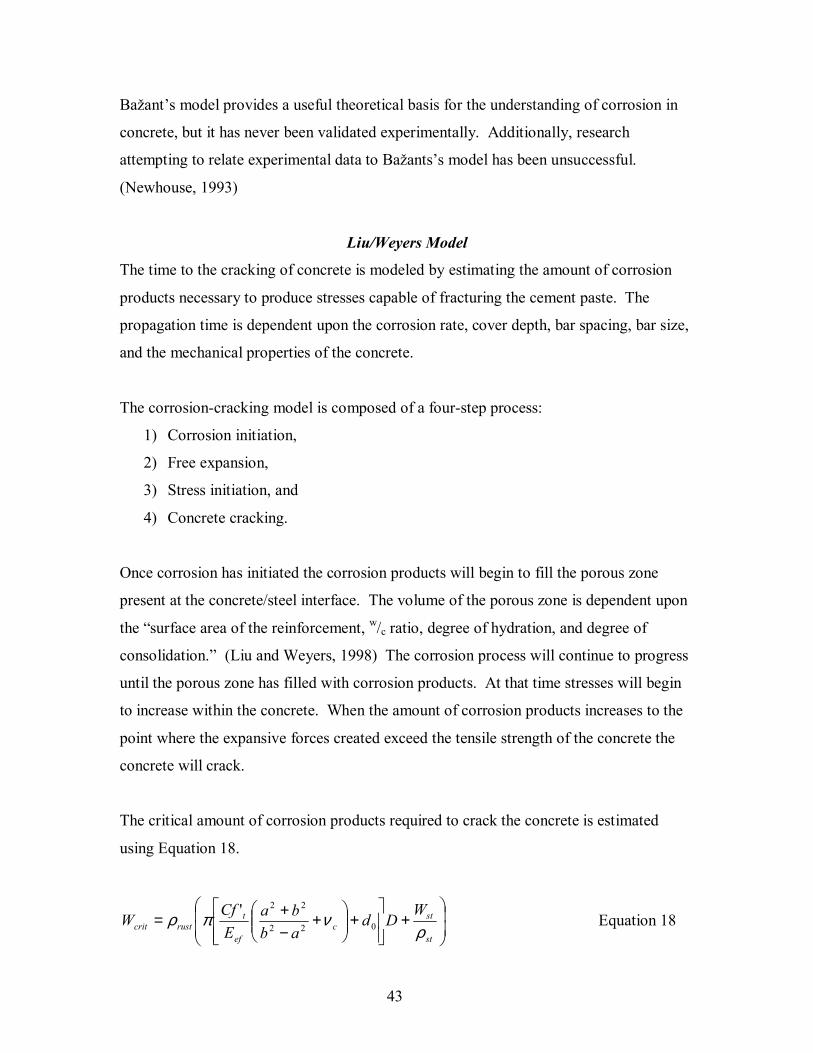
43

Ba�ant�s model provides a useful theoretical basis for the understanding of corrosion in

concrete, but it has never been validated experimentally. Additionally, research

attempting to relate experimental data to Ba�ants�s model has been unsuccessful.

(Newhouse, 1993)

Liu/Weyers Model

The time to the cracking of concrete is modeled by estimating the amount of corrosion

products necessary to produce stresses capable of fracturing the cement paste. The

propagation time is dependent upon the corrosion rate, cover depth, bar spacing, bar size,

and the mechanical properties of the concrete.

The corrosion-cracking model is composed of a four-step process:

1) Corrosion initiation,

2) Free expansion,

3) Stress initiation, and

4) Concrete cracking.

Once corrosion has initiated the corrosion products will begin to fill the porous zone

present at the concrete/steel interface. The volume of the porous zone is dependent upon

the �surface area of the reinforcement, w/c ratio, degree of hydration, and degree of

consolidation.� (Liu and Weyers, 1998) The corrosion process will continue to progress

until the porous zone has filled with corrosion products. At that time stresses will begin

to increase within the concrete. When the amount of corrosion products increases to the

point where the expansive forces created exceed the tensile strength of the concrete the

concrete will crack.

The critical amount of corrosion products required to crack the concrete is estimated

using Equation 18.

+

+

+

−+=

st

stc

ef

trustcrit

WDd

abba

ECf

Wρ

νπρ 022

22' Equation 18

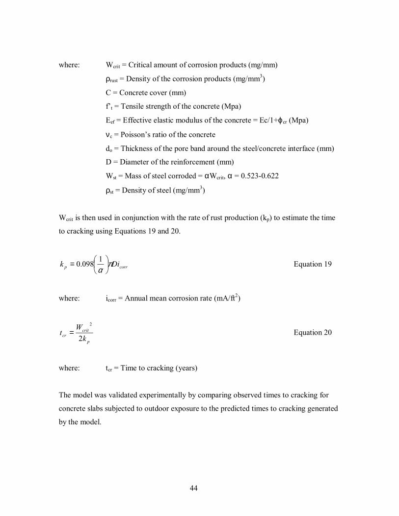
44

where: Wcrit = Critical amount of corrosion products (mg/mm)

ρrust = Density of the corrosion products (mg/mm3)

C = Concrete cover (mm)

f�t = Tensile strength of the concrete (Mpa)

Eef = Effective elastic modulus of the concrete = Ec/1+ϕcr (Mpa)

νc = Poisson�s ratio of the concrete

do = Thickness of the pore band around the steel/concrete interface (mm)

D = Diameter of the reinforcement (mm)

Wst = Mass of steel corroded = αWcrit, α = 0.523-0.622

ρst = Density of steel (mg/mm3)

Wcrit is then used in conjunction with the rate of rust production (kp) to estimate the time

to cracking using Equations 19 and 20.

corrp Dik πα

= 1098.0 Equation 19

where: icorr = Annual mean corrosion rate (mA/ft2)

p

critcr k

Wt

2

2

= Equation 20

where: tcr = Time to cracking (years)

The model was validated experimentally by comparing observed times to cracking for

concrete slabs subjected to outdoor exposure to the predicted times to cracking generated

by the model.

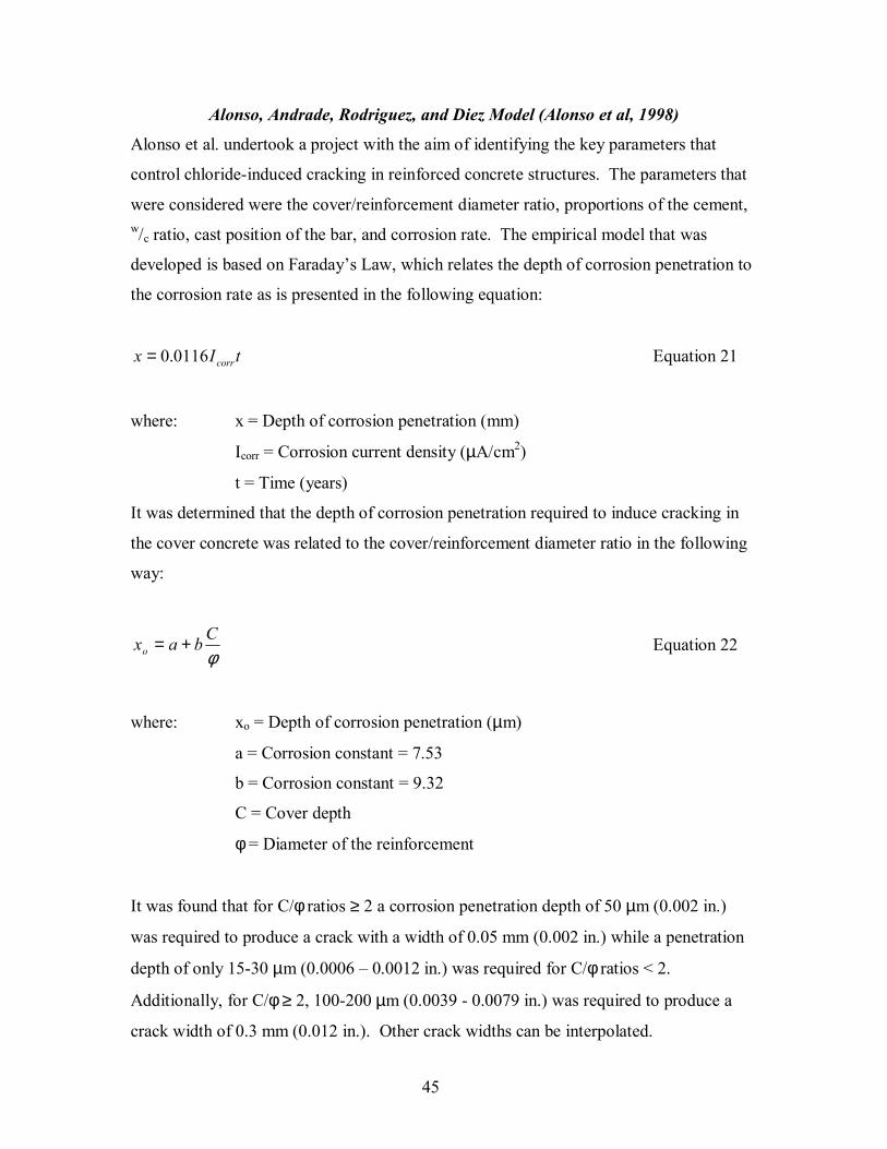
45

Alonso, Andrade, Rodriguez, and Diez Model (Alonso et al, 1998)

Alonso et al. undertook a project with the aim of identifying the key parameters that

control chloride-induced cracking in reinforced concrete structures. The parameters that

were considered were the cover/reinforcement diameter ratio, proportions of the cement, w/c ratio, cast position of the bar, and corrosion rate. The empirical model that was

developed is based on Faraday�s Law, which relates the depth of corrosion penetration to

the corrosion rate as is presented in the following equation:

tIx corr0116.0= Equation 21

where: x = Depth of corrosion penetration (mm)

Icorr = Corrosion current density (µA/cm2)

t = Time (years)

It was determined that the depth of corrosion penetration required to induce cracking in

the cover concrete was related to the cover/reinforcement diameter ratio in the following

way:

φCbaxo += Equation 22

where: xo = Depth of corrosion penetration (µm)

a = Corrosion constant = 7.53

b = Corrosion constant = 9.32

C = Cover depth

φ = Diameter of the reinforcement

It was found that for C/φ ratios ≥ 2 a corrosion penetration depth of 50 µm (0.002 in.)

was required to produce a crack with a width of 0.05 mm (0.002 in.) while a penetration

depth of only 15-30 µm (0.0006 � 0.0012 in.) was required for C/φ ratios < 2.

Additionally, for C/φ ≥ 2, 100-200 µm (0.0039 - 0.0079 in.) was required to produce a

crack width of 0.3 mm (0.012 in.). Other crack widths can be interpolated.

46

It was also determined that higher corrosion rates will require greater depths of corrosion

penetration to produce cracks than lower corrosion rates. This is important mainly in

cases where accelerated experimental results are used to develop cracking models for

actual structures. Another conclusion that was made was that concrete with higher w/c

ratios will propagate cracks slower than concrete with low w/c ratios. This is related to

the ability of corrosion products to diffuse into the concrete. Additionally, top bars tend

to propagate cracks slower than bottom bars. The phenomena were observed and

explained, however, no relationships were developed to quantify their affects.

Torres-Acosta/Sagüés Propagation Model (Torres-Acosta and Sagüés, 2004)

Most corrosion cracking models define the build-up of corrosion products as a uniform

process over the length of the reinforcing bar. However, it is known that concrete

reinforcement in bridge decks typically undergoes local (pitting) corrosion at isolated

locations along the length of the bar. Torres-Acosta and Sagüés investigated the effect

that the size of the anodic region had on the amount of corrosion necessary to crack the

surrounding concrete. It was found that corrosion penetration depths of 0.03 � 0.272 mm

(0.0012 � 0.011 in.) were required to crack the concrete for localized corrosion as

compared to depths of 0.003 � 0.074 mm (0.00012 � 0.0029 in.) for uniform corrosion.

From the experimental data, an empirical equation was developed to estimate the amount

of corrosion required to induce cracking in the concrete, based upon the specimens�

geometry. The developed equation is presented in Equation 23.

2

1011.0

+

≈

LCCxcrit φ

Equation 23

where: xcrit = Critical corrosion penetration (mm)

C = Cover depth (mm)

φ = Reinforcing bar diameter (mm)

L = Length of the anodic region (mm)

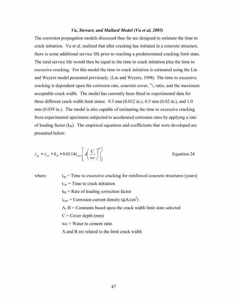
47

Vu, Stewart, and Mullard Model (Vu et al, 2005)

The corrosion propagation models discussed thus far are designed to estimate the time to

crack initiation. Vu et al. realized that after cracking has initiated in a concrete structure,

there is some additional service life prior to reaching a predetermined cracking limit state.

The total service life would then be equal to the time to crack initiation plus the time to

excessive cracking. For this model the time to crack initiation is estimated using the Liu

and Weyers model presented previously. (Liu and Weyers, 1998) The time to excessive

cracking is dependent upon the corrosion rate, concrete cover, w/c ratio, and the maximum

acceptable crack width. The model has currently been fitted to experimental data for

three different crack width limit states: 0.3 mm (0.012 in.), 0.5 mm (0.02 in.), and 1.0

mm (0.039 in.). The model is also capable of estimating the time to excessive cracking

from experimental specimens subjected to accelerated corrosion rates by applying a rate

of loading factor (kR). The empirical equations and coefficients that were developed are

presented below:

×+≈

B

corrRstsp wcCAiktt 0114.01 Equation 24

where: tsp = Time to excessive cracking for reinforced concrete structures (years)

t1st = Time to crack initiation

kR = Rate of loading correction factor

icorr = Corrosion current density (µA/cm2)

A, B = Constants based upon the crack width limit state selected

C = Cover depth (mm)

wc = Water to cement ratio

A and B are related to the limit crack width

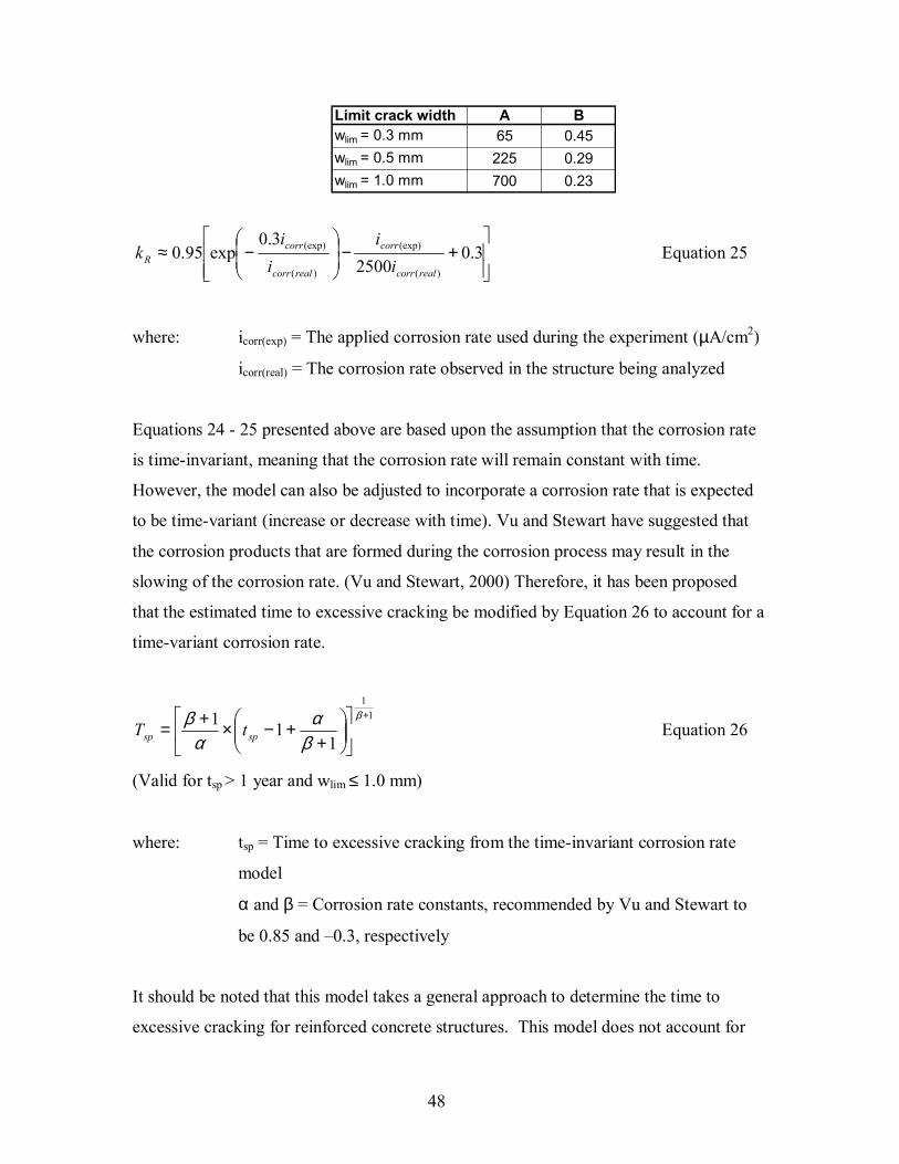
48

+−

−≈ 3.0

25003.0

exp95.0)(

(exp)

)(

(exp)

realcorr

corr

realcorr

corrR i

ii

ik Equation 25

where: icorr(exp) = The applied corrosion rate used during the experiment (µA/cm2)

icorr(real) = The corrosion rate observed in the structure being analyzed

Equations 24 - 25 presented above are based upon the assumption that the corrosion rate

is time-invariant, meaning that the corrosion rate will remain constant with time.

However, the model can also be adjusted to incorporate a corrosion rate that is expected

to be time-variant (increase or decrease with time). Vu and Stewart have suggested that

the corrosion products that are formed during the corrosion process may result in the

slowing of the corrosion rate. (Vu and Stewart, 2000) Therefore, it has been proposed

that the estimated time to excessive cracking be modified by Equation 26 to account for a

time-variant corrosion rate.

11

111 +

+

+−×+=β

βα

αβ

spsp tT Equation 26

(Valid for tsp > 1 year and wlim ≤ 1.0 mm)

where: tsp = Time to excessive cracking from the time-invariant corrosion rate

model

α and β = Corrosion rate constants, recommended by Vu and Stewart to

be 0.85 and �0.3, respectively

It should be noted that this model takes a general approach to determine the time to

excessive cracking for reinforced concrete structures. This model does not account for

Limit crack width A Bwlim = 0.3 mm 65 0.45wlim = 0.5 mm 225 0.29wlim = 1.0 mm 700 0.23

49

the affect of repetitive loading on the crack propagation time period, as would be the case

for a bridge deck. It may be difficult to directly correlate propagation times estimated

from this model to propagation times observed for concrete bridge decks because of this.

Finite Element Analysis of Corrosion Induced Crack Propagation

Several attempts have been made to use commercially available finite element codes to

model corrosion cracking in concrete structures. (Hansen and Saouma, 1999; Molina et

al., 1993; Du et al., 2006) Either a radial expansion of the bar or an internal pressure is

used to model the pressure on the surrounding concrete that is created by the formation of

corrosion products. While the results are promising, a standard, quantitative, and

efficient method has yet to be developed.

50

OBJECTIVE

The objectives of this project are as follows:

• Estimate the service life of bare steel bridge decks with a w/c ratio of 0.45 or a w/(c+p) of 0.45

• Estimate the service life of ECR and alternative reinforcement bridge decks with a w/c ratio of 0.45 or a w/(c+p) of 0.45

• Estimate the cost of maintaining these bridge decks for a service life of 100 years

• Evaluate the affect of using alternative reinforcements with a w/(c+p) of 0.45 on

service life cost

It is important for VDOT to be able to reasonably estimate the service lives of bridge

decks containing bare, epoxy-coated, and alternative reinforcements in order to calculate

the life cycle costs for the different alternatives. Currently, VDOT has a reasonable

estimate of the service life that is obtainable for bare steel bridge decks with w/c ratios of

0.47, but the affect of reducing the w/c ratio to 0.45 on service life is not known.

Additionally, bridge decks containing ECR have not been in service for a long enough

period of time to know what their long-term performance will be. It is the objective of

this project to develop estimates that will enable different corrosion prevention

alternatives to be compared with regards to their ability to extend the service life of

bridge decks and reduce total life cycle costs.

51

SCOPE

The scope of this project is limited to those corrosion prevention systems that are

currently in place or being investigated in Virginia. These systems include bridge decks

containing bare steel reinforcement and ECR with w/c or w/(c+p) ratios of 0.45 and 0.47.

Additionally, the use of alternative reinforcements that are under consideration, such as

MMFX-2, stainless steel, and galvanized steel, will be investigated. The practice of

extending the service life of bridge decks needing repair and rehabilitation using Latex

Modified Concrete (LMC), Microsilica Concrete (MSC), and Polymer Concrete (PC)

overlays will also be addressed and incorporated into the life cycle cost analysis.

Bridge deck service lives will be estimated using a service life model based upon Fick�s

second law of diffusion described by Equation 1. To simplify the complex diffusion

process and to provide conservative estimations, the surface chloride concentration and

diffusion coefficient values will be determined from samples taken from in service decks,

generally greater than 15 years of age. The model will take advantage of Monte Carlo

simulation to provide more realistic results by taking into account the variability of

surface and corrosion initiation chloride concentration values, cover depths, and diffusion

coefficients.

52

METHODS AND MATERIALS

Bridge Deck Selection

The original research plan called for the survey of 40 bridge decks. The distribution of

bridge deck types was to be as follows: 10 bare steel with w/c = 0.47, 15 ECR with w/c =

0.45, and 15 ECR with w/(c+p) = 0.45. VDOT officials compiled a list of potential bridge

decks that indicated whether or not pozzolans were used in the deck, the type of

reinforcement present, the age of the structure, and if the bridge had been overlaid. It

was important to select bridge decks that had not received overlays because an overlay

would affect the chloride concentrations in the deck and skew the calculated diffusion

coefficients. 40 bridges that met the research plan criteria were randomly selected from

the VDOT prepared list. Additionally, the bridges selected for surveying were evenly

dispersed across the 6 climatic zones in Virginia. The survey locations are presented in

Figure 3.

Figure 3 � Surveyed Bridge Locations

It was necessary to survey bridge decks from all six climatic zones because research

conducted over a three-year period from 2001 to 2003 indicated that the chloride

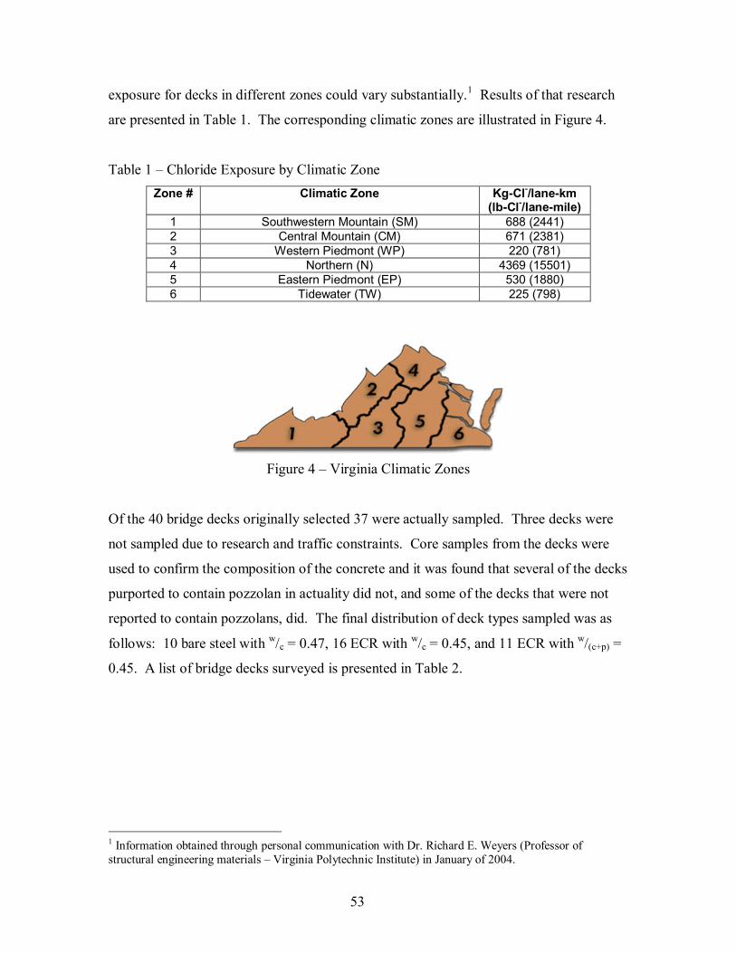
53

exposure for decks in different zones could vary substantially.1 Results of that research

are presented in Table 1. The corresponding climatic zones are illustrated in Figure 4.

Table 1 � Chloride Exposure by Climatic Zone Zone # Climatic Zone Kg-Cl-/lane-km

(lb-Cl-/lane-mile) 1 Southwestern Mountain (SM) 688 (2441) 2 Central Mountain (CM) 671 (2381) 3 Western Piedmont (WP) 220 (781) 4 Northern (N) 4369 (15501) 5 Eastern Piedmont (EP) 530 (1880) 6 Tidewater (TW) 225 (798)

Figure 4 � Virginia Climatic Zones

Of the 40 bridge decks originally selected 37 were actually sampled. Three decks were

not sampled due to research and traffic constraints. Core samples from the decks were

used to confirm the composition of the concrete and it was found that several of the decks

purported to contain pozzolan in actuality did not, and some of the decks that were not

reported to contain pozzolans, did. The final distribution of deck types sampled was as

follows: 10 bare steel with w/c = 0.47, 16 ECR with w/c = 0.45, and 11 ECR with w/(c+p) =

0.45. A list of bridge decks surveyed is presented in Table 2.

1 Information obtained through personal communication with Dr. Richard E. Weyers (Professor of structural engineering materials � Virginia Polytechnic Institute) in January of 2004.

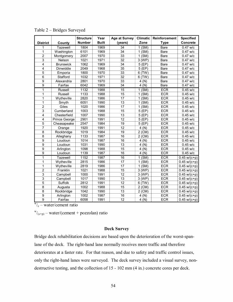
54

Table 2 � Bridges Surveyed

w/c � water/cement ratio w/(c+p) � water/(cement + pozzolan) ratio

Deck Survey

Bridge deck rehabilitation decisions are based upon the deterioration of the worst-span-

lane of the deck. The right-hand lane normally receives more traffic and therefore

deteriorates at a faster rate. For that reason, and due to safety and traffic control issues,

only the right-hand lanes were surveyed. The deck survey included a visual survey, non-

destructive testing, and the collection of 15 - 102 mm (4 in.) concrete cores per deck.

District CountyStructureNumber

YearBuilt

Age at Survey (years)

Climatic Zone

ReinforcementType

Specified Concrete

1 Tazewell 1804 1969 34 1 (SM) Bare 0.47 w/c1 Washington 6101 1969 34 1 (SM) Bare 0.47 w/c2 Montgomery 2007 1970 33 1 (SM) Bare 0.47 w/c3 Nelson 1021 1971 32 3 (WP) Bare 0.47 w/c4 Brunswick 1062 1969 34 5 (EP) Bare 0.47 w/c4 Dinwiddie 2049 1968 35 5 (EP) Bare 0.47 w/c5 Emporia 1800 1970 33 6 (TW) Bare 0.47 w/c6 Stafford 1032 1971 32 6 (TW) Bare 0.47 w/c9 Alexandria 2801 1970 33 4 (N) Bare 0.47 w/c9 Fairfax 6042 1969 34 4 (N) Bare 0.47 w/c1 Russell 1132 1988 15 1 (SM) ECR 0.45 w/c1 Russell 1133 1988 15 1 (SM) ECR 0.45 w/c1 Wytheville 2820 1986 17 1 (SM) ECR 0.45 w/c1 Smyth 6051 1990 13 1 (SM) ECR 0.45 w/c2 Giles 1020 1986 17 1 (SM) ECR 0.45 w/c3 Cumberland 1003 1988 15 5 (EP) ECR 0.45 w/c4 Chesterfield 1007 1990 13 5 (EP) ECR 0.45 w/c4 Prince George 2901 1991 12 5 (EP) ECR 0.45 w/c5 Cheasapeake 2547 1984 19 5 (EP) ECR 0.45 w/c7 Orange 1920 1991 12 4 (N) ECR 0.45 w/c8 Rockbridge 1019 1984 19 2 (CM) ECR 0.45 w/c8 Alleghany 1133 1987 16 2 (CM) ECR 0.45 w/c9 Loudoun 1014 1987 16 4 (N) ECR 0.45 w/c9 Loudoun 1031 1990 13 4 (N) ECR 0.45 w/c9 Arlington 1098 1988 15 4 (N) ECR 0.45 w/c9 Loudoun 1139 1987 16 4 (N) ECR 0.45 w/c1 Tazewell 1152 1987 16 1 (SM) ECR 0.45 w/(c+p)1 Wytheville 2815 1986 17 1 (SM) ECR 0.45 w/(c+p)1 Wytheville 2819 1986 17 1 (SM) ECR 0.45 w/(c+p)2 Franklin 1021 1988 15 3 (WP) ECR 0.45 w/(c+p)3 Campbell 1000 1991 12 3 (WP) ECR 0.45 w/(c+p)3 Campbell 1017 1990 13 3 (WP) ECR 0.45 w/(c+p)5 Suffolk 2812 1991 12 6 (TW) ECR 0.45 w/(c+p)8 Augusta 1002 1988 15 2 (CM) ECR 0.45 w/(c+p)8 Rockbridge 1042 1990 13 2 (CM) ECR 0.45 w/(c+p)9 Arlington 1002 1987 16 4 (N) ECR 0.45 w/(c+p)9 Fairfax 6058 1991 12 4 (N) ECR 0.45 w/(c+p)

55

Visual Survey

The following data was gathered for each bridge deck during the visual survey:

• The length and width of the right traffic lane were measured.

• Patched areas within the right-hand lane were measured and recorded.

• A visual determination of the wheel path locations was made.

• A crack survey was performed consisting of recording the number, length, width

and orientation of the cracks in each span.

• Other structural data including the type of superstructure (i.e. steel, prestressed,

and cast-in-place concrete), structure type (continuous or simply supported), and

the girder spacing was recorded. Additionally, the presence of stay-in-place

forms, the superelevation condition, and the skew angle of the deck were

recorded.

Non-destructive Field Testing

The following non-destructive tests were conducted during the field survey:

• Cover depth determinations for the top mat of reinforcing steel. 40-80

measurements were taken per span at 4-foot (1.2 m) intervals in the wheel paths

using a Profometer 3 cover depth meter. If the span length did not allow for 40

measurements to be taken at 4-foot (1.2 m) intervals the interval was reduced to 2

feet (0.6 m).

• The right-hand lane was sounded using the chain drag method to determine

delaminated areas.

• Copper-copper half-cell (CSE) measurements were taken at the same locations as

the cover depth measurements.

• Corrosion current densities were determined at 4-6 locations using an unguarded

three-electrode linear polarization (3LP) instrument.

• Concrete resistivity measurements were taken at 9 locations using a four-probe

Wenner apparatus.

56

Deck Cores and Laboratory Testing

The concrete cores were taken within the wheel paths on the deck as that is the critical

deterioration area. Three of the cores were taken for petrographic analysis purposes and

did not contain reinforcing steel. Of the remaining 12, all contained reinforcing steel and

3 were taken directly over cracks in the deck. After the cores were removed the water on

the surface resulting from the coring process was allowed to dry off and then the cores

were wrapped in two layers of 102 µm (4-mil) polyethylene and one layer of aluminum

foil. The cores were then wrapped in a protective layer of duct tape. This was done to

preserve the in-place moisture content of the concrete samples until they could be

analyzed in the lab.

The following tests were conducted in the laboratory on the cores taken from the bridge

decks:

• Chloride concentrations were determined in accordance to ASTM C 1152-97 at

the following seven depths for each concrete core sample: 0.5 in. (12.7 mm), 0.75

in. (19.05 mm), 1.0 in. (25.4 mm), 1.25 in. (31.75 mm), 1.5 in. (38.1 mm), at the

depth of the reinforcement, and below the reinforcement.

• Concrete resistivity measurements were taken at depths of 0.25 in. (6.35 mm),

0.75 in. (19.05 mm), 1.25 in. (31.75 mm), and below the reinforcement. They

were taken both parallel and perpendicular to the reinforcing bar.

• Concrete permeability data were obtained in accordance to ASTM C 1202.

• Concrete density/absorption data were determined in accordance to ASTM C 642.

• The condition of the reinforcement was recorded including: the number of

holidays (ECR only), the number of damaged areas (ECR only), coating thickness

measurements (ECR only), peel tests (ECR only), and estimated % rusted surface

area.

• Concrete moisture contents were determined for each core.

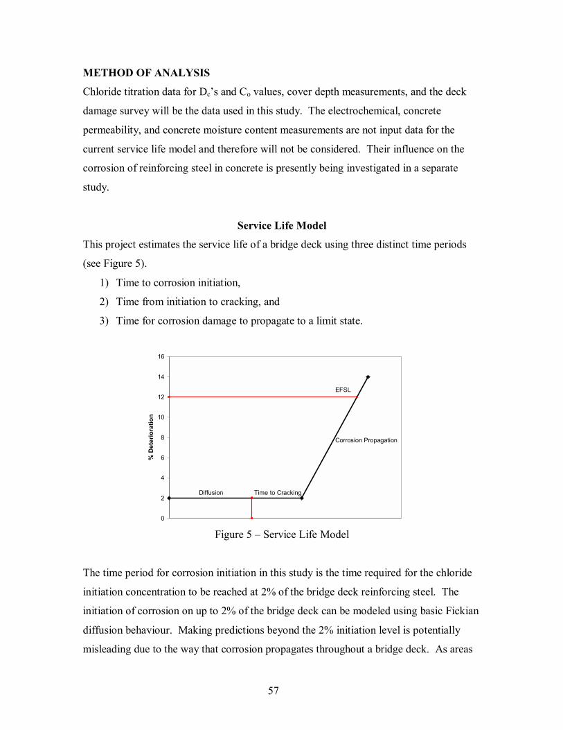
57

METHOD OF ANALYSIS

Chloride titration data for Dc�s and Co values, cover depth measurements, and the deck

damage survey will be the data used in this study. The electrochemical, concrete

permeability, and concrete moisture content measurements are not input data for the

current service life model and therefore will not be considered. Their influence on the

corrosion of reinforcing steel in concrete is presently being investigated in a separate

study.

Service Life Model

This project estimates the service life of a bridge deck using three distinct time periods

(see Figure 5).

1) Time to corrosion initiation,

2) Time from initiation to cracking, and

3) Time for corrosion damage to propagate to a limit state.

Figure 5 � Service Life Model

The time period for corrosion initiation in this study is the time required for the chloride

initiation concentration to be reached at 2% of the bridge deck reinforcing steel. The

initiation of corrosion on up to 2% of the bridge deck can be modeled using basic Fickian

diffusion behaviour. Making predictions beyond the 2% initiation level is potentially

misleading due to the way that corrosion propagates throughout a bridge deck. As areas

0

2

4

6

8

10

12

14

16

% D

eter

iora

tion

Diffusion Time to Cracking

Corrosion Propagation

EFSL

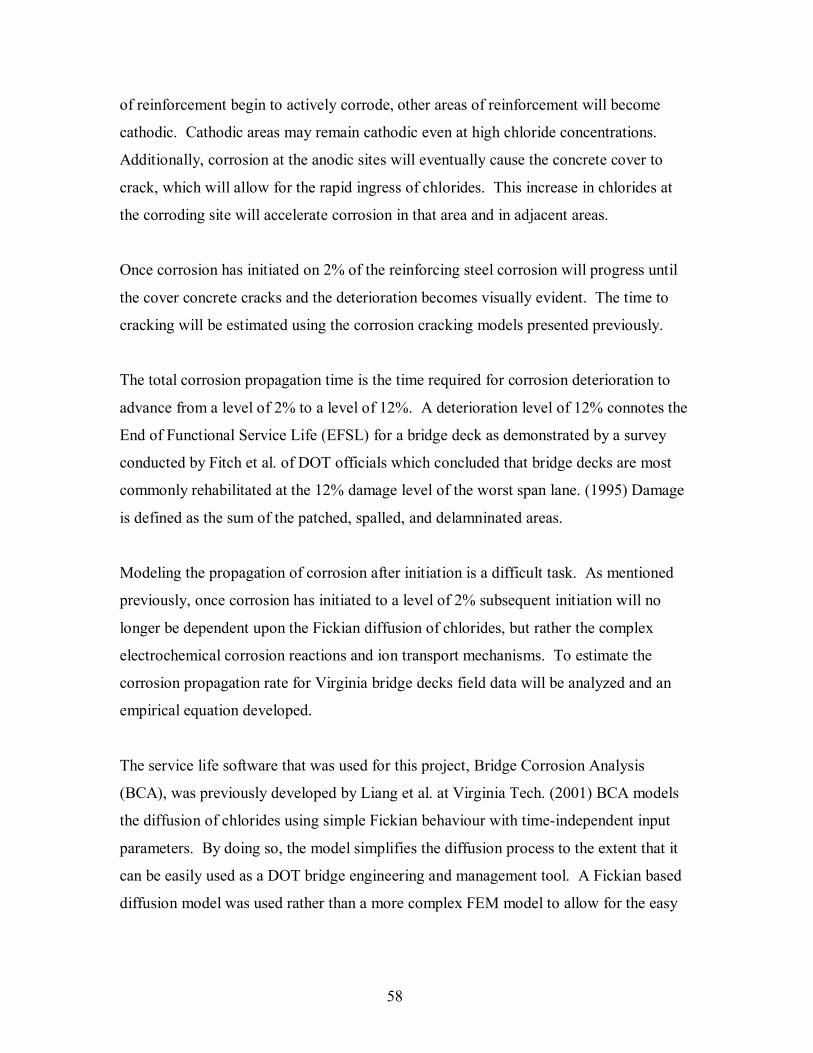
58

of reinforcement begin to actively corrode, other areas of reinforcement will become

cathodic. Cathodic areas may remain cathodic even at high chloride concentrations.

Additionally, corrosion at the anodic sites will eventually cause the concrete cover to

crack, which will allow for the rapid ingress of chlorides. This increase in chlorides at

the corroding site will accelerate corrosion in that area and in adjacent areas.

Once corrosion has initiated on 2% of the reinforcing steel corrosion will progress until

the cover concrete cracks and the deterioration becomes visually evident. The time to

cracking will be estimated using the corrosion cracking models presented previously.

The total corrosion propagation time is the time required for corrosion deterioration to

advance from a level of 2% to a level of 12%. A deterioration level of 12% connotes the

End of Functional Service Life (EFSL) for a bridge deck as demonstrated by a survey

conducted by Fitch et al. of DOT officials which concluded that bridge decks are most

commonly rehabilitated at the 12% damage level of the worst span lane. (1995) Damage

is defined as the sum of the patched, spalled, and delamninated areas.

Modeling the propagation of corrosion after initiation is a difficult task. As mentioned

previously, once corrosion has initiated to a level of 2% subsequent initiation will no

longer be dependent upon the Fickian diffusion of chlorides, but rather the complex

electrochemical corrosion reactions and ion transport mechanisms. To estimate the

corrosion propagation rate for Virginia bridge decks field data will be analyzed and an

empirical equation developed.

The service life software that was used for this project, Bridge Corrosion Analysis

(BCA), was previously developed by Liang et al. at Virginia Tech. (2001) BCA models

the diffusion of chlorides using simple Fickian behaviour with time-independent input

parameters. By doing so, the model simplifies the diffusion process to the extent that it

can be easily used as a DOT bridge engineering and management tool. A Fickian based

diffusion model was used rather than a more complex FEM model to allow for the easy

59

incorporation of the stochastic nature of the input variables. BCA was developed as an

Excel module, which was added to the standard Microsoft Office package.

Deterministic vs. Probabilistic Service Life Models

Service life models can be either deterministic or probabilistic. Deterministic service life

models estimate the EFSL for a bridge deck using an average value for the various input

parameters. Conversly, probabilistic models incorporate the stochastic nature of the

variables into service life estimates. Previous research concerning the service life

modeling of bridge decks has shown that a deterministic approach to the problem will

result in a significant overestimation of service life. (Kirkpatrick, 2001) Thus, the

software used in this project will make use of Monte Carlo statistical resampling

techniques to allow for the integration of input parameter variability into the model.

Monte Carlo Simulation

Monte Carlo Simulation (MCS) is defined as �any method, which solves a problem by

generating suitable random numbers and observing that fraction of the numbers obeying

some property or properties.� (Weisstein, 2006) MCS is used for complex problems that

cannot be easily solved using standard deterministic models. It takes into account the

statistical nature of the input parameters by randomly selecting numerical values from a

provided data set (simple bootstrapping) or based upon a known distribution for each data

set (parametric bootstrapping). As mentioned previously, the range of the input variables

is defined by the data gathered for each individual bridge deck. It is also important to

ensure that the number of sampling iterations used is adequate. For a small number of

iterations (<20) the range of the expected service life for a bridge deck is quite large, but

as the number of iterations increases the range will narrow to an acceptable level. It has

been shown that for 10,000 iterations the service life prediction will converge to a near

constant value when the distributions of the input variables are adequately defined.

(Kirkpatrick, 2001)

60

Parametric Bootstrapping

Parametric bootstrapping is the process by which numerical values are randomly

generated for a given variable based upon a provided range of values and distribution.

For example, cover depth measurements have been shown to be normally distributed.

Therefore, the range of possible values for cover depths can be defined by the mean and

standard deviation of the cover depth data set. Once the distribution has been identified

the service life model will randomly generate values for the cover depth based on the

developed variable parameters.

Simple Bootstrapping

In contrast to parametric bootstrapping, simple bootstrapping will only sample values

from a provided data set and will not incorporate any known or assumed distribution.

Simple bootstrapping is useful in situations where large quantities of data (> 15 data

points) are available, but if the data set is fairly limited simple bootstrapping may not

accurately reflect the variability actually present.

Modeling the Time to Corrosion Initiation

The first step in estimating the time to corrosion initiation is calculating Dca from the

chloride profiles developed from the bridge deck samples.

Apparent Diffusion Coefficient (Dca) Calculation

Dca is calculated using Fick�s second law of diffusion as described by Equation 1. The

diffusion portion of the BCA service life model was validated by comparing the results

with two other diffusion programs. (Zemajtis, 1998 and Sagues2)

The diffusion model back calculates Dca using chloride concentration data obtained from

the concrete samples taken from the bridge decks. The surface chloride concentration is

one of the most important factors in calculating Dca. It has been shown that the chloride

concentration profiles for bridge deck cores reach a maximum at a depth of

approximately ½ in. (12.7 mm) during the summer after 5 � 10 years of exposure to 2 Information obtained through personal communication with Dr. Alberto A. Sagues (Professor of Civil Engineering - University of South Florida) in August of 2005.

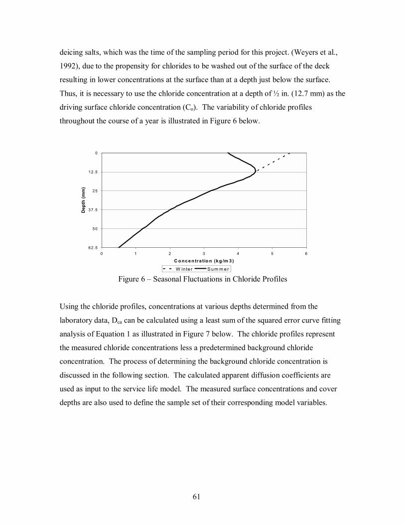
61

deicing salts, which was the time of the sampling period for this project. (Weyers et al.,

1992), due to the propensity for chlorides to be washed out of the surface of the deck

resulting in lower concentrations at the surface than at a depth just below the surface.

Thus, it is necessary to use the chloride concentration at a depth of ½ in. (12.7 mm) as the

driving surface chloride concentration (Co). The variability of chloride profiles

throughout the course of a year is illustrated in Figure 6 below.

Figure 6 � Seasonal Fluctuations in Chloride Profiles

Using the chloride profiles, concentrations at various depths determined from the

laboratory data, Dca can be calculated using a least sum of the squared error curve fitting

analysis of Equation 1 as illustrated in Figure 7 below. The chloride profiles represent

the measured chloride concentrations less a predetermined background chloride

concentration. The process of determining the background chloride concentration is

discussed in the following section. The calculated apparent diffusion coefficients are

used as input to the service life model. The measured surface concentrations and cover

depths are also used to define the sample set of their corresponding model variables.

0

12 .5

25

37 .5

50

62 .50 1 2 3 4 5 6

C o nc e n tra tio n (k g /m 3 )

Dep

th (m

m)

W in te r S um m er

62

Figure 7 � Determination of Apparent Diffusion Coefficient

The Graphical User Interface (GUI) used by BCA to calculate Dca is presented below.

Figure 8 � BCA GUI - Dca Input Form

Structure #: 1-1804 Core: C1

0

20

40

60

800 1 2 3 4 5 6 7 8

Cx,t(kg/m 3)

Dep

th(m

m)

Measurements Fitted Dif fusion Curve

63

The input data can be in either SI or U.S. Customary units. The Dc seed value is the

initial value that is used to estimate the diffusion curve. The value is user defined and for

most cases it does not matter what the value is. However, for bridge decks with low

diffusion rates it is necessary to use a low Dc seed value (i.e. < 1). Using the input data

BCA estimates the diffusion coefficient and generates a chloride profile along with a

fitted diffusion curve as illustrated in Figure 9.

Figure 9 � BCA Output - Dca

Background Chloride Concentration Determination

Chlorides initially present within a concrete mixture either contained within the cement

paste or the aggregate are known as bound chlorides. The concentration of bound

chlorides is relatively uniform and varies between bridge decks, but are in general

relatively low. It has been argued that bound chlorides may in some cases enter the

concrete pore water over the life of a structure due to corrosion-related equilibrium

64

requirements, but for this study the bound chlorides have been taken to remain bound due

to the nature of the concrete, cement, and aggregates.

The background chloride concentration for the individual bridge decks was determined

by investigating the chloride titrations that were conducted on specimens taken from

below the reinforcement. These specimens were generally at depths greater than 75 mm

(3in.). For the quality of the concrete specified and the average age of the bridge decks

investigated, it is unlikely that chlorides would have diffused to this depth; therefore, any

chlorides present are expected to be background (bound) chlorides. It should also be

noted that if the chlorides present below the reinforcement were the result of diffusion

then the reinforcement should reflect very high levels of corrosion, which was not the

case for any of the decks investigated.

The background chloride concentration was calculated to be the average of the chloride

concentrations taken from below the reinforcement. The background chloride

concentration was then subtracted from the chloride profile prior to the determination of

Dca. Background concentrations were determined for each bridge deck independently, as

it is not uncommon for different concrete mixtures to have significantly different

background chloride concentrations.

The calculated background concentration was also verified by investigating the chloride

profiles. The chloride profiles will become asymptotic at the background chloride

concentration value as illustrated in Figure 10. For the case presented below the

background chloride concentration would be taken as 0.2 kg/m3 (.38 lbs/cy).

65

Figure 10 � Background Chloride Concentration Determination Example

Adjusting Diffusion Coefficients for Time Dependency

As described previously, the diffusion properties of concrete are time-dependent. To

account for time effects in the measured Dca values three diffusion models were used to

estimate the decay of Dc over time. The time-dependency equations for those models are

presented below. Pozzolan containing bridge decks were taken to have a 25%

replacement rate of cement with fly ash (FA).

Mangat and Molloy (1994) m

ic tDD −= Equation 27

where: 6.05.2 −

=

cwm Equation 28

Using the above equation the calculated values of m for 0.45 w/c and 0.47 w/c OPC bridge

decks were 0.525 and 0.575, respectively. To calculate a value of m for a bridge deck

containing FA the FA is ignored in this equation. A typical concrete mixture with a 0.45 w/c contains approximately 375 kg/m3 (632 lbs/cy) of cementitious material and 169

kg/m3 (285 lbs/cy) of water. Twenty-five percent replacement of the cement with FA is

0

10

20

30

40

50

60

70

80

90

1000 0.2 0.4 0.6 0.8 1 1.2 1.4 1.6 1.8

Concentration (kg/m3)

Dep

th (m

m)

66

typical for VDOT bridge deck concrete mixtures yielding 169 kg (373 lbs) of water to

281 kg (620 lbs) of cement or a w/c of 0.6. Using that ratio a value of 0.9 was calculated

for m.

Bamforth (1999) n

ca atD = Equation 29

Bamforth estimated values of n for a 0.45 w/c concrete mixtures. The values for OPC and

FA concrete are �0.264 and �0.70, respectively.

Life � 365 m

refref t

tDtD

=)( Equation 30

where:

++=

50%

50%4.02.0 SlagFAm Equation 31

Using the above equation values of m for OPC and FA concrete were calculated to be 0.2

and 0.4, respectively.

The equations presented above were used to model the decay of Dc over time. However,

the diffusion coefficients that are calculated from the field data are the apparent diffusion

coefficients (Dca) not the actual diffusion coefficients for the concrete at the time of

sampling. Dca can be defined as the average Dc value over the life of a structure.

Therefore, Dca will have a higher value than Dc at any given point in time with the margin

of difference between Dca and Dc narrowing with time. This relationship is presented for

each of the three models in Figures 11 � 13 for 0.45 w/c FA concrete.

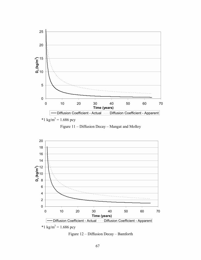
67

*1 kg/m3 = 1.686 pcy

Figure 11 � Diffusion Decay � Mangat and Molloy

*1 kg/m3 = 1.686 pcy

Figure 12 � Diffusion Decay � Bamforth

0

5

10

15

20

25

0 10 20 30 40 50 60 70Time (years)

Dc (k

g/m

3 )

Diffusion Coefficient - Actual Diffusion Coefficient - Apparent

0

2

4

6

8

10

12

14

16

18

20

0 10 20 30 40 50 60 70Time (years)

Dc (k

g/m

3 )

Diffusion Coefficient - Actual Diffusion Coefficient - Apparent

68

*1 kg/m3 = 1.686 pcy

Figure 13 � Diffusion Decay � Life � 365

Using the three diffusion decay models presented above the Dca curve can be forced to fit

through a known measured value at a specified time and then the actual Dc can be

calculated for that particular sample at any time in the past or a prediction can be made

for the future value of Dc. For example the diffusion comparison presented in Figure 13

above for the Life � 365 model was determined using a known Dca value of 6.0 mm2/yr

(0.009 in2/yr) at an age of 12 years. The steps that were used to generate the diffusion

decay plot were as follows:

1) A random initial Dc value was selected and the diffusion curve was generated

based upon that value and the value for m that was selected based upon the

concrete mixture proportions.

2) The Dca diffusion curve was then generated by averaging the Dc values over the

life of the structure.

3) The Dca curve was then checked to ensure that it passed through the known point

of 6.0 mm2/yr (0.009 in2/yr) at an age of 12 years.

0

2

4

6

8

10

12

14

0 10 20 30 40 50 60 70Time (years)

Dc (k

g/m

3 )

Diffusion Coefficient - Apparent Diffusion Coefficient - Actual

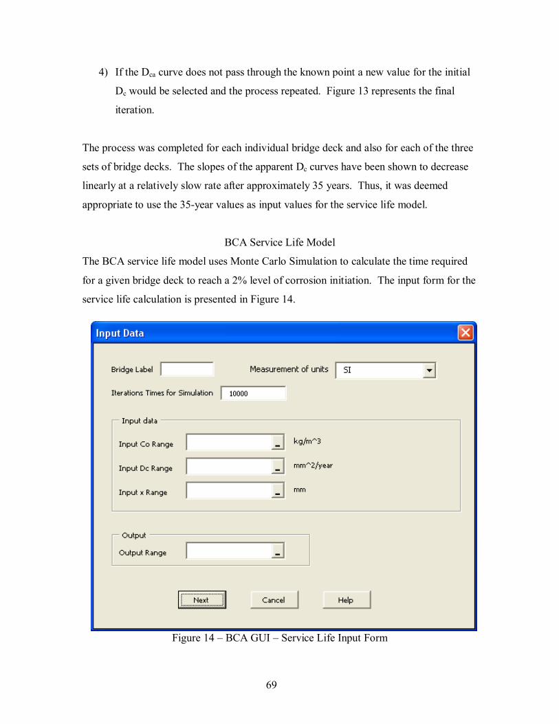
69

4) If the Dca curve does not pass through the known point a new value for the initial

Dc would be selected and the process repeated. Figure 13 represents the final

iteration.

The process was completed for each individual bridge deck and also for each of the three

sets of bridge decks. The slopes of the apparent Dc curves have been shown to decrease

linearly at a relatively slow rate after approximately 35 years. Thus, it was deemed

appropriate to use the 35-year values as input values for the service life model.

BCA Service Life Model

The BCA service life model uses Monte Carlo Simulation to calculate the time required

for a given bridge deck to reach a 2% level of corrosion initiation. The input form for the

service life calculation is presented in Figure 14.

Figure 14 � BCA GUI � Service Life Input Form

70

BCA accepts a set of input values from which it will randomly select a value for each

variable using the simple bootstrapping method. Once the necessary input data has been

provided the program will prompt the user for information regarding the chloride

threshold concentrations. The chloride threshold input form is presented in Figure 15.

71

Figu

re 1

5 �

BC

A C

hlor

ide

Thre

shol

d In

put F

orm

72

The chloride threshold values that will be used in the service life calculation can be

specified in one of four ways.

1) Default values for 5 different corrosion protection methods can be used that are

specified by BCA,

2) User can specify minimum, maximum, and mode values for the chloride threshold

and BCA will generate values according to a triangular distribution,

3) User can specify a mean and standard deviation of the threshold values and BCA

will generate values according to a normal distribution, or

4) User can specify a set of threshold values and BCA will sample directly from that

set.

The first three options use parametric bootstrapping to generate and select chloride

threshold values while the fourth method uses simple bootstrapping to sample directly

from a provided data set.

After the chloride threshold information has been provided BCA will calculate the time

required for corrosion to initiate for that set of input values and chloride thresholds. The

process is repeated for the number of specified iterations up to a maximum of 65000

iterations. The computer routine that is used is illustrated in Figure 16.

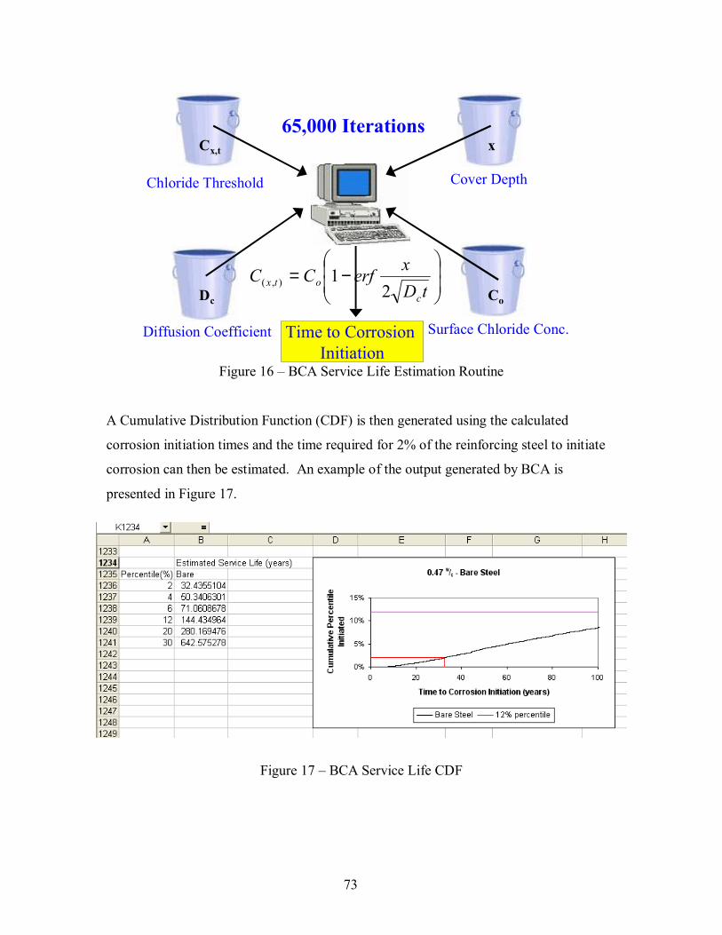
73

Figure 16 � BCA Service Life Estimation Routine

A Cumulative Distribution Function (CDF) is then generated using the calculated

corrosion initiation times and the time required for 2% of the reinforcing steel to initiate

corrosion can then be estimated. An example of the output generated by BCA is

presented in Figure 17.

Figure 17 � BCA Service Life CDF

Diffusion Coefficient

Chloride Threshold Cover Depth

Time to Corrosion Initiation

Dc Co

Cx,t x

Surface Chloride Conc.

65,000 Iterations

−=

tDxerfCC

cotx 2

1),(

74

Estimating the Time to Corrosion Cracking for Bare Steel

After the time required for corrosion to initiate has been calculated the time to corrosion

cracking must be added. The time for cracking to initiate has been calculated for each of

the models presented previously. The values for the parameters used were selected to

represent the characteristics of a typical bridge deck in Virginia.

Ba�ant Model

Parameters:

D = 15.875 mm; s = 203.4 mm ρcor = 3.6 g/cm2

jr = 5.3797x10-5 g/cm2days L = 50.8 mm f�t = 3.3 Mpa

Eef = 9000 Mpa ν = 0.18

Calculated time to crack initiation: 24 days

Liu/Weyers Model

Parameters:

C = 52.2 mm D = 15.875 mm do = .0125 mm

f�t = 3.3 Mpa Eef = 9000 Mpa icorr = 2 mA/ft2

νc = 0.18 α = 0.523 � 0.622 ρst = 7.86 mg/mm3

ρrust = 3.6 mg/mm3

Calculated time to crack initiation: 2.08 � 2.80 years

Alonso, Andrade, Rodriguez, and Diez Model

Penetration depth of 50 � 200 µm


Vu, Stewart, and Mullard Model

Parameters:

A = 62, 225, 700 B = 0.45, 0.29, 0.23 C = 52.2 mm w/c = 0.45 icorr(exp) = 100 µA/cm2 icorr(real) = 2.14 µA/cm2

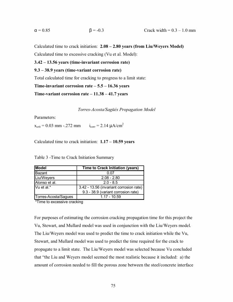
75

α = 0.85 β = -0.3 Crack width = 0.3 � 1.0 mm

Calculated time to crack initiation: 2.08 � 2.80 years (from Liu/Weyers Model)

Calculated time to excessive cracking (Vu et al. Model):

3.42 � 13.56 years (time-invariant corrosion rate)

9.3 � 38.9 years (time-variant corrosion rate)

Total calculated time for cracking to progress to a limit state:

Time-invariant corrosion rate � 5.5 � 16.36 years

Time-variant corrosion rate � 11.38 � 41.7 years

Torres-Acosta/Sagüés Propagation Model

Parameters:

xcrit = 0.03 mm -.272 mm icorr = 2.14 µA/cm2


Table 3 -Time to Crack Initiation Summary

For purposes of estimating the corrosion cracking propagation time for this project the

Vu, Stewart, and Mullard model was used in conjunction with the Liu/Weyers model.

The Liu/Weyers model was used to predict the time to crack initiation while the Vu,

Stewart, and Mullard model was used to predict the time required for the crack to

propagate to a limit state. The Liu/Weyers model was selected because Vu concluded

that �the Liu and Weyers model seemed the most realistic because it included: a) the

amount of corrosion needed to fill the porous zone between the steel/concrete interface

Model Time to Crack Initiation (years)Bazant 0.07Liu/Weyers 2.08 - 2.80Alonso et al. 2.0 - 8.5Vu et al.* 3.42 - 13.56 (invariant corrosion rate)

9.3 - 38.9 (variant corrosion rate)Torres-Acosta/Sagues 1.17 - 10.59*Time to excessive cracking

76

(free expansion); and b) the reduction with time of the rate of rust production when

determining the critical tensile stress needed to cause cover cracking.� (Vu, 2003)

The corrosion products were taken to be a composition of Fe(OH)3 and Fe(OH)2 and the

crack width limit state was taken to be 0.3 mm (0.012 in.). A crack width limit state of

0.3 mm (0.012 in.) was selected because it has been suggested that crack widths of less

than 0.3 mm (0.012 in.) have little to no effect on the ingress of chlorides into the

concrete. (Atimay and Ferguson, 1974) Using these parameters the time to crack

initiation was calculated to be 2.40 years and the time for crack propagation was

calculated to be 3.42 years yielding a total corrosion cracking propagation time of 5.82

years. For simplicity the total crack propagation time that will be used to estimate bridge

deck service life is 6 years.

Estimating the Time to Corrosion Cracking for ECR

It is known that the epoxy coating on a reinforcing bar will slow the corrosion rate for

that bar. Several research projects indicate that the additional propagation time provided

by the epoxy coating is approximately 5 years. (Brown, 2002; McDonald, 1998)

Therefore, the crack propagation time for ECR bridge decks will be taken as 11 years as

compared to the 6 years provided by bare steel.

Estimating the Propagation Time of Corrosion for Bare Steel Bridge Decks

The propagation of corrosion is a complex process that cannot be described by simple

Fickian behaviour. BCA is not currently capable of determining the propagation period.

Therefore, the corrosion propagation time has been estimated using empirical data.

To estimate the corrosion propagation time for bare steel bridge decks in Virginia those

bridge decks that reflected the most damage during the intial survey were resurveyed

three years later. A total of 7 bridge decks were resurveyed and their effective

deterioration rates calculated. It was found that the deterioration rate of a bridge deck is

related to the amount of initial damage on that deck. The relationship is presented in

Figure 18.

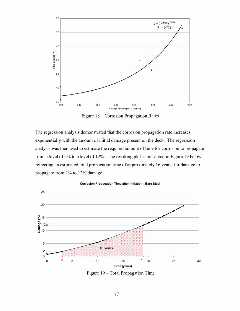
77

Figure 18 � Corrosion Propagation Rates

The regression analysis demonstrated that the corrosion propagation rate increases

exponentially with the amount of initial damage present on the deck. The regression

analysis was then used to estimate the required amount of time for corrosion to propagate

from a level of 2% to a level of 12%. The resulting plot is presented in Figure 19 below

reflecting an estimated total propagation time of approximately 16 years, for damage to

propagate from 2% to 12% damage.

Figure 19 � Total Propagation Time

y = 0.4196e3.9106x

R2 = 0.7731

0.0

1.0

2.0

3.0

4.0

5.0

6.0

0.00 0.10 0.20 0.30 0.40 0.50 0.60 0.70

Change in Damage - 1 Year (%)

Initi

al D

amag

e (%

)

Corrosion Propagation Time after Initiation - Bare Steel

0

5

10

15

20

25

0 5 10 15 20 25 30

Time (years)

Dam

age

(%)

3

2

12

19

16 years

78

The time required to reach a specific level of deterioration can also be calculated using

the following equation:

( ) 34.345.138.1%61.8 −−+= ionDeterioratriorationTimeToDete Equation 32

The time calculated will be the time for corrosion to progress from a deterioration level

of 2% to the specified level.

Estimating the Propagation Time of Corrosion for ECR Bridge Decks

Estimating the corrosion propagation time for ECR bridge decks using empirical data is

not possible due to their relatively young age and low levels of deterioration. The effect

that the epoxy coating will have on the rate of corrosion is not fully understood. It is

suspected that the corrosion rate will be lower due to the electrical isolation provided by

the coating. However, if the coating debonds from the steel substrate it is possible for

corrosion to progress rapidly underneath the coating. To estimate the propagation rate for

ECR the deterioration rate for one bridge deck located in Blacksburg was analyzed.

A visual survey3 of structure number 8003 (Prices Fork Road of Rt. 460) was conducted

during the summer of 1996. At that time the right hand traffic lane reflected a

deterioration level of 0.5%. A VDOT bridge inspection conducted in August of 2001

determined that the deterioration had progressed to a level of 8.2%. The bridge deck was

rehabilitated during the summer of 2003 due to excessive damage. VDOT work orders

report that a total of 105 sq yds (87.8 m2) were patched prior to overlaying the deck. It is

common construction practice to remove some additional concrete surrounding

deteriorated areas to ensure that all of the damaged area is removed. This additional

patched area is estimated to be 20% of the total patched area yielding a total deteriorated

area of 84 sq yds or 756 sq ft (70.2 m2).

3 Information obtained through personal communication with Professor Richard Weyers of the Virginia Polytechnic Institute and State University, November 2006.

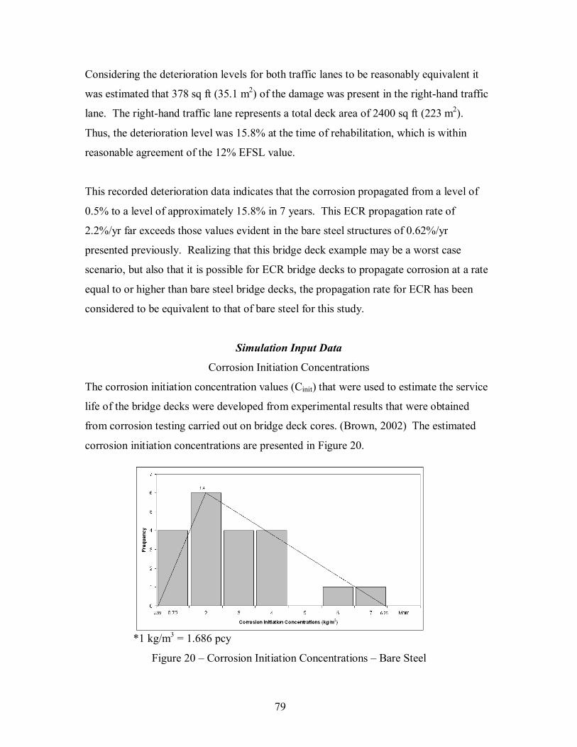
79

Considering the deterioration levels for both traffic lanes to be reasonably equivalent it

was estimated that 378 sq ft (35.1 m2) of the damage was present in the right-hand traffic

lane. The right-hand traffic lane represents a total deck area of 2400 sq ft (223 m2).

Thus, the deterioration level was 15.8% at the time of rehabilitation, which is within

reasonable agreement of the 12% EFSL value.

This recorded deterioration data indicates that the corrosion propagated from a level of

0.5% to a level of approximately 15.8% in 7 years. This ECR propagation rate of

2.2%/yr far exceeds those values evident in the bare steel structures of 0.62%/yr

presented previously. Realizing that this bridge deck example may be a worst case

scenario, but also that it is possible for ECR bridge decks to propagate corrosion at a rate

equal to or higher than bare steel bridge decks, the propagation rate for ECR has been

considered to be equivalent to that of bare steel for this study.

Simulation Input Data

Corrosion Initiation Concentrations

The corrosion initiation concentration values (Cinit) that were used to estimate the service

life of the bridge decks were developed from experimental results that were obtained

from corrosion testing carried out on bridge deck cores. (Brown, 2002) The estimated

corrosion initiation concentrations are presented in Figure 20.

*1 kg/m3 = 1.686 pcy

Figure 20 � Corrosion Initiation Concentrations � Bare Steel

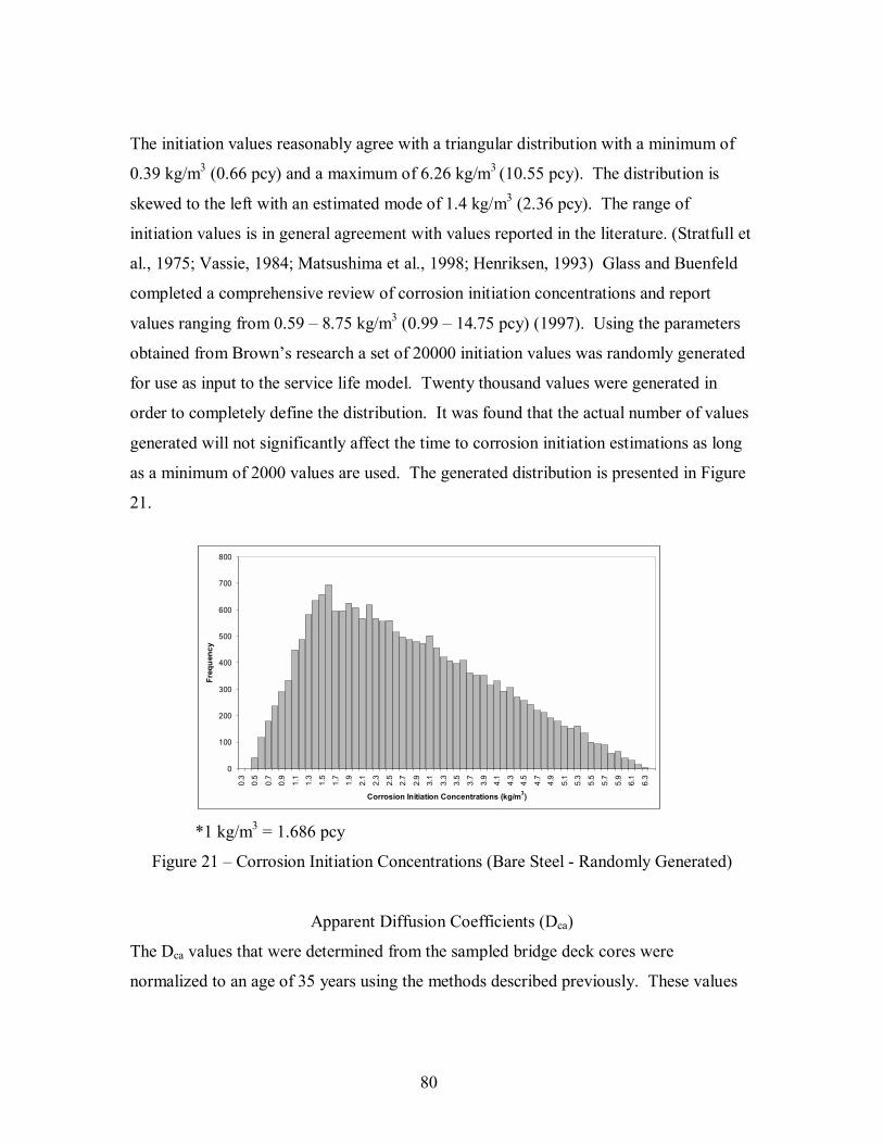
80

The initiation values reasonably agree with a triangular distribution with a minimum of

0.39 kg/m3 (0.66 pcy) and a maximum of 6.26 kg/m3 (10.55 pcy). The distribution is

skewed to the left with an estimated mode of 1.4 kg/m3 (2.36 pcy). The range of

initiation values is in general agreement with values reported in the literature. (Stratfull et

al., 1975; Vassie, 1984; Matsushima et al., 1998; Henriksen, 1993) Glass and Buenfeld

completed a comprehensive review of corrosion initiation concentrations and report

values ranging from 0.59 � 8.75 kg/m3 (0.99 � 14.75 pcy) (1997). Using the parameters

obtained from Brown�s research a set of 20000 initiation values was randomly generated

for use as input to the service life model. Twenty thousand values were generated in

order to completely define the distribution. It was found that the actual number of values

generated will not significantly affect the time to corrosion initiation estimations as long

as a minimum of 2000 values are used. The generated distribution is presented in Figure

21.

*1 kg/m3 = 1.686 pcy

Figure 21 � Corrosion Initiation Concentrations (Bare Steel - Randomly Generated)

Apparent Diffusion Coefficients (Dca)

The Dca values that were determined from the sampled bridge deck cores were

normalized to an age of 35 years using the methods described previously. These values

0

100

200

300

400

500

600

700

800

0.3

0.5

0.7

0.9

1.1

1.3

1.5

1.7

1.9

2.1

2.3

2.5

2.7

2.9

3.1

3.3

3.5

3.7

3.9

4.1

4.3

4.5

4.7

4.9

5.1

5.3

5.5

5.7

5.9

6.1

6.3

Corrosion Initiation Concentrations (kg/m3)

Freq

uenc

y

81

were then used in the service life estimations. The actual values used will be presented in

the Results section.

Surface Chloride Concentrations (Co)

The Co values used in the service life model were the measured values taken from the

deck cores at a depth of ½ in. (12.7 mm) minus the estimated background chloride

concentration. In instances where the chloride concentration reached a maximum at a

depth greater than ½ in. (12.7 mm) the higher concentration was used for Co.

Cover Depths (x)

The cover depths determined from pachometer measurements were used as the input to

the service life model. The pachometer measurements were validated by comparing the

field measurements at the core locations to the actual cover depths that were measured in

the laboratory for the 10 - 0.45 w/c bridge decks. The field measurements differed from

the actual values by as little as 1% to a maximum of 13%. The average difference was

5%, which is an insignificant amount when used in the service life model.

82

RESULTS

Bridge Deck Damage Surveys

The results of the deck damage surveys are presented in Tables 4-5. The damage levels

presented are the total of both the measured visual damage and the damage determined

through sounding for the right-hand traffic lane (critical traffic lane). The 0.47 w/c bridge

decks were resurveyed 3 years after the initial damage survey to provide data on

corrosion propagation rates.

Table 4 � 0.47 w/c Bridge Deck Damage Surveys

Table 5 � 0.45 w/c and 0.45 w/c+p Bridge Deck Damage Surveys

Structure # Age at Survey % Damaged 2003 Age at Survey % Damaged 20061-1804 34 3.3 37 5.31-6101 34 0.0 37 0.02-2007 33 0.8 36 2.33-1021 32 0.2 35 0.24-1062 34 0.0 37 0.04-2049 35 0.2 38 0.75-1800 33 1.8 36 3.36-1032 32 0.0 35 0.09-2801 33 1.7 36 3.09-6042 34 1.1 37 1.1

0.47 w/c Bridge Decks

Structure # Age at Survey % Damaged 2003 Structure # Age at Survey % Damaged 20031-1132 15 0.0 1-1152 16 0.01-1133 15 0.0 1-2815 17 0.01-2820 17 0.0 1-2819 17 0.01-6051 13 0.0 2-1021 15 0.02-1020 17 0.0 3-1000 12 0.03-1003 15 0.0 5-2812 12 0.04-1007 13 0.0 8-1002 15 0.04-2901 12 0.0 8-1042 13 0.35-2547 19 0.0 9-1002 16 0.07-1920 12 0.3 9-6058 12 0.08-1019 19 0.08-1133 16 0.09-1014 15 0.09-1031 13 0.19-1098 15 0.09-1139 16 0.0

0.45 w/c Bridge Decks 0.45 w/(c+p) Bridge Decks

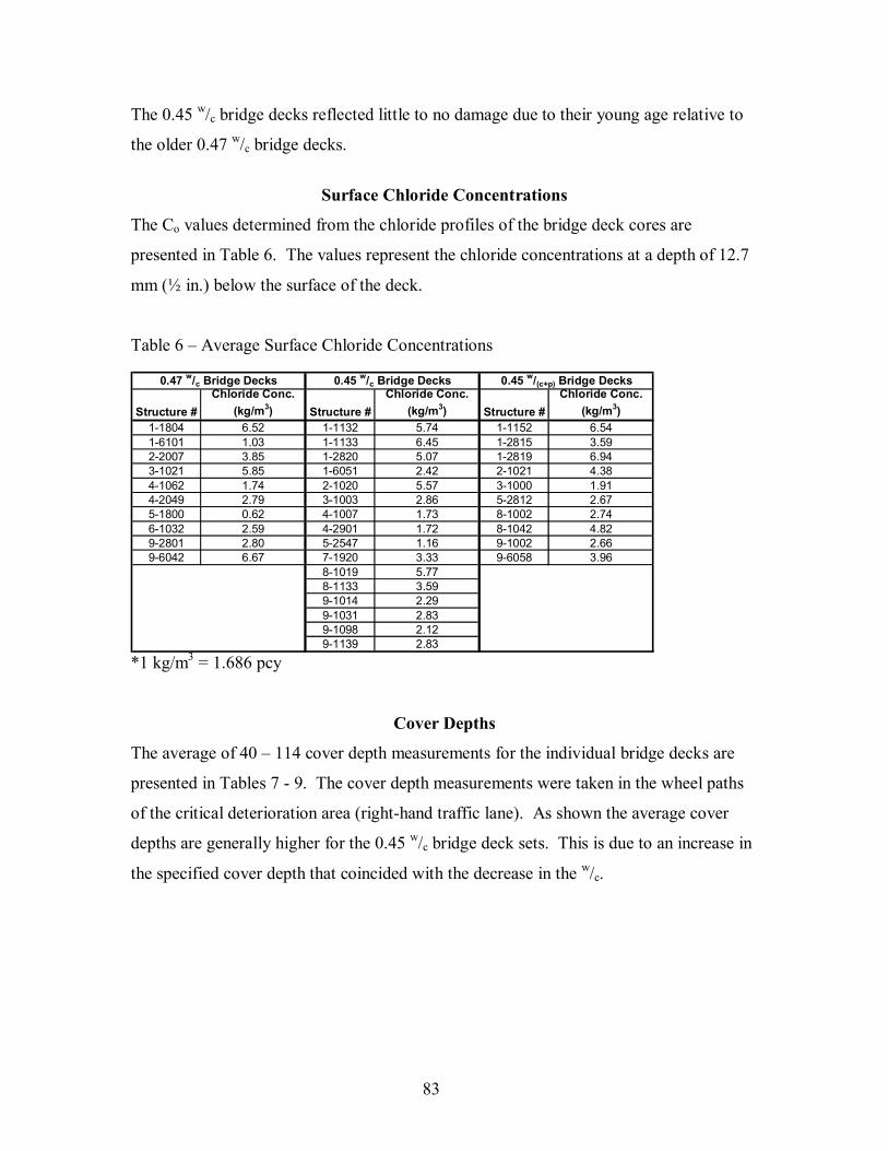
83

The 0.45 w/c bridge decks reflected little to no damage due to their young age relative to

the older 0.47 w/c bridge decks.

Surface Chloride Concentrations

The Co values determined from the chloride profiles of the bridge deck cores are

presented in Table 6. The values represent the chloride concentrations at a depth of 12.7

mm (½ in.) below the surface of the deck.

Table 6 � Average Surface Chloride Concentrations

*1 kg/m3 = 1.686 pcy

Cover Depths

The average of 40 � 114 cover depth measurements for the individual bridge decks are

presented in Tables 7 - 9. The cover depth measurements were taken in the wheel paths

of the critical deterioration area (right-hand traffic lane). As shown the average cover

depths are generally higher for the 0.45 w/c bridge deck sets. This is due to an increase in

the specified cover depth that coincided with the decrease in the w/c.

Structure #Chloride Conc.

(kg/m3) Structure #Chloride Conc.

(kg/m3) Structure #Chloride Conc.

(kg/m3)1-1804 6.52 1-1132 5.74 1-1152 6.541-6101 1.03 1-1133 6.45 1-2815 3.592-2007 3.85 1-2820 5.07 1-2819 6.943-1021 5.85 1-6051 2.42 2-1021 4.384-1062 1.74 2-1020 5.57 3-1000 1.914-2049 2.79 3-1003 2.86 5-2812 2.675-1800 0.62 4-1007 1.73 8-1002 2.746-1032 2.59 4-2901 1.72 8-1042 4.829-2801 2.80 5-2547 1.16 9-1002 2.669-6042 6.67 7-1920 3.33 9-6058 3.96

8-1019 5.778-1133 3.599-1014 2.299-1031 2.839-1098 2.129-1139 2.83

0.47 w/c Bridge Decks 0.45 w/c Bridge Decks 0.45 w/(c+p) Bridge Decks

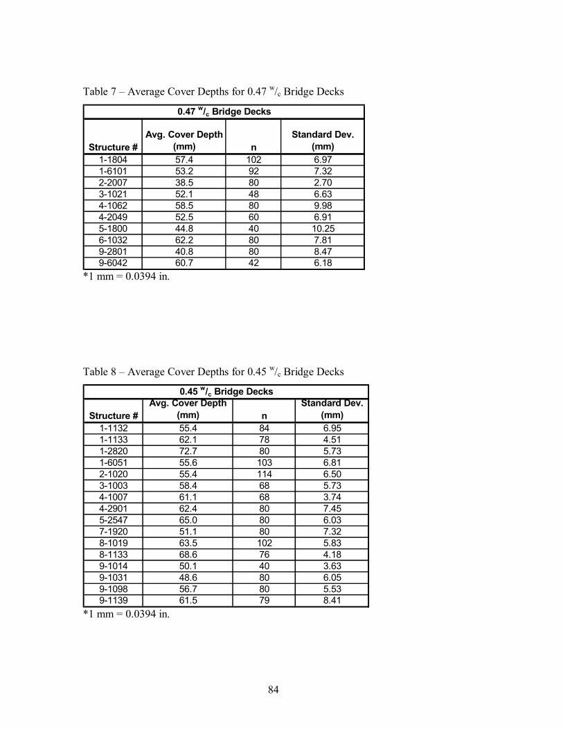
84

Table 7 � Average Cover Depths for 0.47 w/c Bridge Decks

*1 mm = 0.0394 in.

Table 8 � Average Cover Depths for 0.45 w/c Bridge Decks

*1 mm = 0.0394 in.

Structure #Avg. Cover Depth

(mm) nStandard Dev.

(mm)1-1804 57.4 102 6.971-6101 53.2 92 7.322-2007 38.5 80 2.703-1021 52.1 48 6.634-1062 58.5 80 9.984-2049 52.5 60 6.915-1800 44.8 40 10.256-1032 62.2 80 7.819-2801 40.8 80 8.479-6042 60.7 42 6.18



(mm) nStandard Dev.

(mm)1-1132 55.4 84 6.951-1133 62.1 78 4.511-2820 72.7 80 5.731-6051 55.6 103 6.812-1020 55.4 114 6.503-1003 58.4 68 5.734-1007 61.1 68 3.744-2901 62.4 80 7.455-2547 65.0 80 6.037-1920 51.1 80 7.328-1019 63.5 102 5.838-1133 68.6 76 4.189-1014 50.1 40 3.639-1031 48.6 80 6.059-1098 56.7 80 5.539-1139 61.5 79 8.41


85

Table 9 � Average Cover Depths for 0.45 w/c+p Bridge Decks

*1 mm = 0.0394 in.

Diffusion Coefficients

Apparent diffusion coefficients were calculated for the sampled bridge decks using Fick�s

second law of diffusion. The Dca values were then normalized to an age of 35 years using

the methods described previously. The average calculated Dca values and the average Dca

values projected at an age of 35 years are presented in Table 10.

Table 10 � Average Diffusion Coefficients

*1 mm2/yr = 0.0015 in2/yr

Structure #Apparent Dc

(mm2/yr)Dc35

(mm2/yr) Structure #Apparent Dc

(mm2/yr)Dc35

(mm2/yr) Structure #Apparent Dc

(mm2/yr)Dc35

(mm2/yr)1-1804 35.74 36.35 1-1132 38.26 30.09 1-1152 2.3 1.521-6101 4.55 4.63 1-1133 82.64 64.98 1-2815 3.73 2.542-2007 6.30 6.35 1-2820 14.85 12.08 1-2819 5.35 3.633-1021 20.68 20.68 1-6051 51.72 39.19 2-1021 3.49 2.224-1062 3.63 3.69 2-1020 17.49 14.23 3-1000 1.96 1.124-2049 6.15 6.30 3-1003 46.02 36.19 5-2812 6.39 3.655-1800 7.97 8.04 4-1007 26.47 20.06 8-1002 5.09 3.256-1032 4.39 4.39 4-2901 26.18 19.43 8-1042 5.77 3.439-2801 4.72 4.76 5-2547 5.53 4.64 9-1002 11.82 7.799-6042 13.05 13.28 7-1920 56.44 41.88 9-6058 7.09 4.05

8-1019 30.69 25.768-1133 24.06 19.269-1014 19.74 15.529-1031 36.82 27.909-1098 9.28 7.299-1139 40.98 32.80

0.47 w/c Bridge Decks 0.45 w/(c+p) Bridge Decks0.45 w/c Bridge Decks


(mm) nStandard Dev.

(mm)1-1152 63.1 60 14.251-2815 63.9 103 5.501-2819 67.3 114 6.172-1021 61.8 48 4.153-1000 52.3 50 5.075-2812 63.8 40 4.128-1002 57.7 68 6.498-1042 58.7 56 11.129-1002 66.2 82 8.699-6058 55.9 40 4.34

0.45 w/(c+p) Bridge Decks

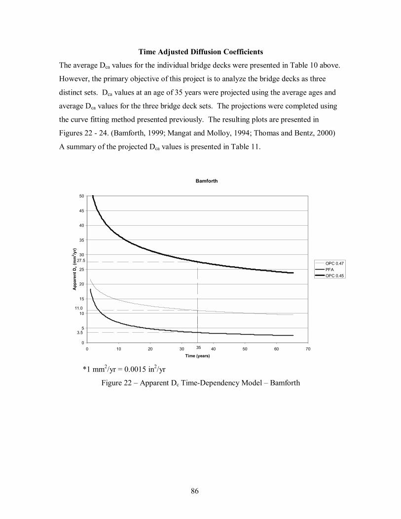
86

Time Adjusted Diffusion Coefficients

The average Dca values for the individual bridge decks were presented in Table 10 above.

However, the primary objective of this project is to analyze the bridge decks as three

distinct sets. Dca values at an age of 35 years were projected using the average ages and

average Dca values for the three bridge deck sets. The projections were completed using

the curve fitting method presented previously. The resulting plots are presented in

Figures 22 - 24. (Bamforth, 1999; Mangat and Molloy, 1994; Thomas and Bentz, 2000)

A summary of the projected Dca values is presented in Table 11.

*1 mm2/yr = 0.0015 in2/yr

Figure 22 � Apparent Dc Time-Dependency Model � Bamforth

Bamforth

0

5

10

15

20

25

30

35

40

45

50

0 10 20 30 40 50 60 70Time (years)

App

aren

t Dc (

mm

2 /yr)

OPC 0.47PFAOPC 0.45

35

11.0

3.5

27.5

87

*1 mm2/yr = 0.0015 in2/yr

Figure 23 � Apparent Dc Time-Dependency Model � Life 365

*1 mm2/yr = 0.0015 in2/yr

Figure 24 � Apparent Dc Time-Dependency Model � Mangat and Molloy

Mangat and Molloy(First exposure at 6 months)

0

5

10

15

20

25

30

35

40

0 10 20 30 40 50 60 70

Time (years)

App

. Dc

(mm

2 /yr)

OPC .45PFAOPC .47

35

10.8

3.0

22.7

Life 365(First exposure at 6 months)

0

5

10

15

20

25

30

35

40

0 10 20 30 40 50 60 70

Time (years)

App

. Dc

(mm

2 /yr)

OPC .45PFAOPC .47

35

11

28.5

4.1

88

Table 11 � Apparent Dc Time-Dependent Model Data

*1 mm2/yr = 0.0015 in2/yr

By projecting the Dca values for the three sets to an age of 35 years the influence of the

three types of concrete may be compared at an equivalent age. As shown in Table 11, at

an age of 35 years the decks containing a pozzolan with a w/c ratio of 0.45 have the lowest

Dca values and the decks with no pozzolan and a w/c of 0.45 have the highest Dca value. It

is interesting that the 0.45 w/c OPC decks have significantly higher Dca values than the

0.47 w/c OPC decks. The implication is that the newer 0.45 w/c decks may not have been

constructed as specified or the older decks were constructed with properties in excess of

their specifications. In either case it is clear that the older decks are reflecting better

diffusion properties than the newer decks. It is not possible to draw any conclusions

concerning the construction quality of the bridge decks containing pozzolan as the

decreased Dca values are most likely attributable to the addition of pozzolan. In all cases

the Dca will continue to decrease with time to a limited extent and the pozzolan concrete

decks will decrease at a faster rate than both of the OPC bridge deck sets.

Using the projected Dca values of the three bridge deck sets it is estimated that the bridge

decks with 0.45 w/c concrete will have a reduction in Dca of 21%, and the pozzolan decks

will have a reduction of 39% at an age of 35 years.

Service Life Model Input Data

Histograms of the input data were developed for each of the three bridge deck sets to

investigate the distributions of the input parameters. The histograms for the three bridge

deck sets are presented in Figures 25 - 33.

Concrete TypeAverage Age

(years) Apparent Dc (mm2/yr) Mangat and Molloy Bamforth Life 365 AverageOPC 0.47 36.4 10.9 11.1 11.0 11.0 11.0OPC 0.45 15.1 33.3 22.7 27.5 28.5 26.2PFA 25% 14.4 5.7 3.0 3.5 4.1 3.5

Predicted Apparent Dc at 35 years of age

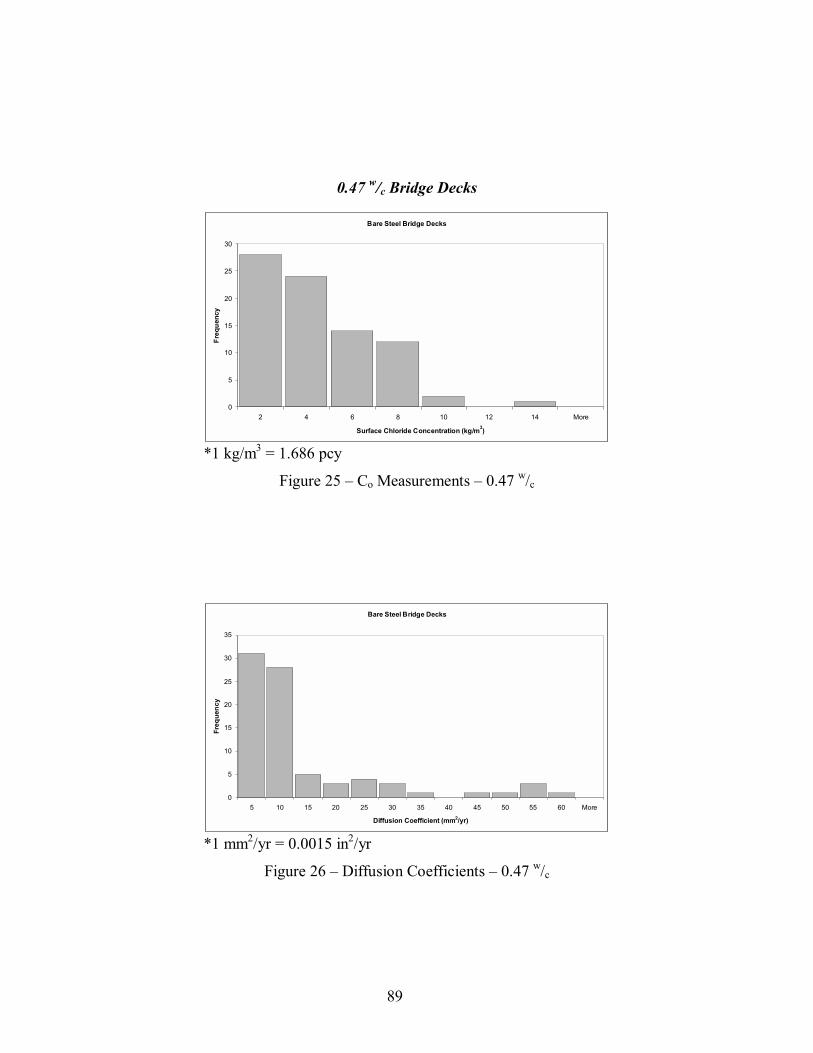
89


*1 kg/m3 = 1.686 pcy

Figure 25 � Co Measurements � 0.47 w/c

*1 mm2/yr = 0.0015 in2/yr

Figure 26 � Diffusion Coefficients � 0.47 w/c

Bare Steel Bridge Decks

0

5

10

15

20

25

30

2 4 6 8 10 12 14 More

Surface Chloride Concentration (kg/m3)

Freq

uenc

y


0

5

10

15

20

25

30

35

5 10 15 20 25 30 35 40 45 50 55 60 More

Diffusion Coefficient (mm2/yr)

Freq

uenc

y

90

* 1 mm = 0.039 in.

Figure 27 �Cover Depth Measurements � 0.47 w/c

0.45 w/c � No Pozzolan Bridge Decks

*1 kg/m3 = 1.686 pcy

Figure 28 � Surface Chloride Concentrations � 0.45 w/c No Pozzolan

0.45 w/c - No Pozzolan

0

5

10

15

20

25

30

1 2 3 4 5 6 7 8 More

Co (kg/m3)

Freq

uenc

y


0

20

40

60

80

100

120

140

160

25 30 35 40 45 50 55 60 65 70 75 80 85 More

Cover Depth Measurements (mm)

Freq

uenc

y

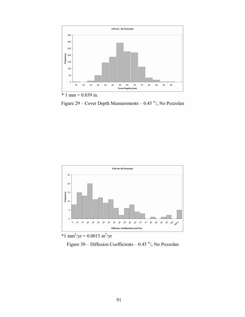
91

* 1 mm = 0.039 in.

Figure 29 � Cover Depth Measurements � 0.45 w/c No Pozzolan

*1 mm2/yr = 0.0015 in2/yr

Figure 30 � Diffusion Coefficients � 0.45 w/c No Pozzolan

0.45 w/c - No Pozzolan

0

50

100

150

200

250

300

350

30 35 40 45 50 55 60 65 70 75 80 85 90 95Cover Depths (mm)

Freq

uenc

y

0.45 w/c No Pozzolan

0

5

10

15

20

25

5 10 15 20 25 30 35 40 45 50 55 60 65 70 75 80 85 90 9510

0More

Diffusion Coeffiecients (mm2/yr)

Freq

uenc

y

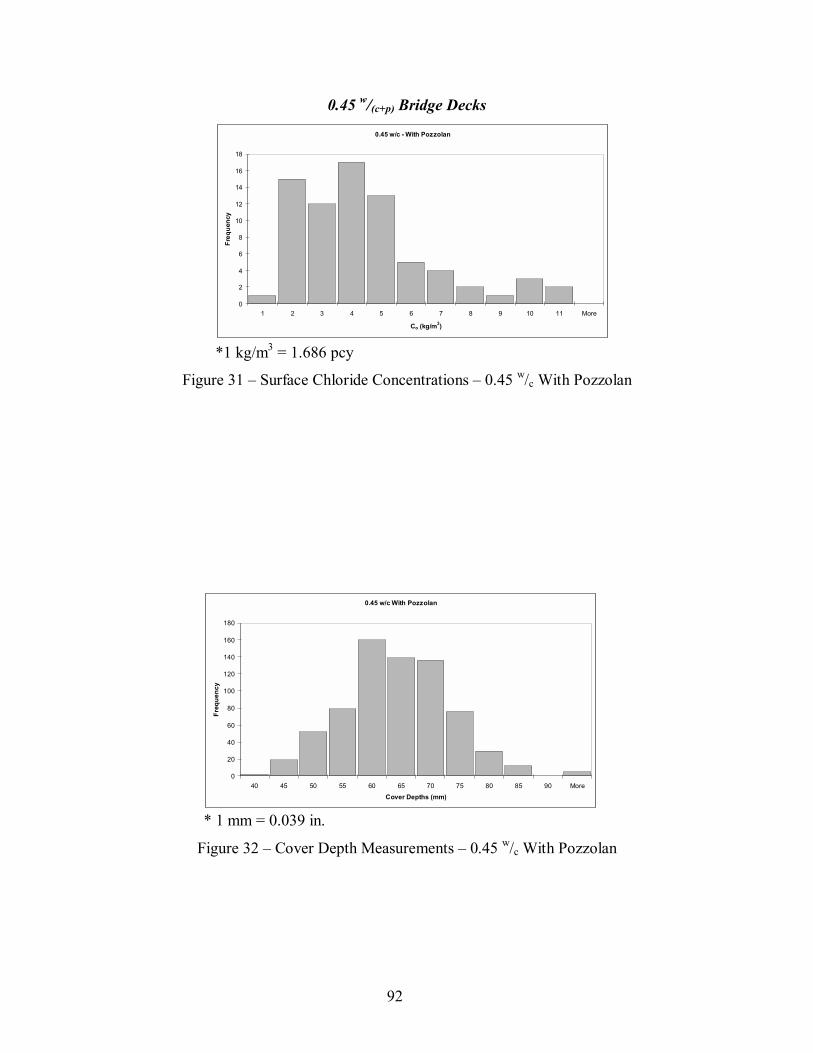
92

0.45 w/(c+p) Bridge Decks

*1 kg/m3 = 1.686 pcy

Figure 31 � Surface Chloride Concentrations � 0.45 w/c With Pozzolan

* 1 mm = 0.039 in.

Figure 32 � Cover Depth Measurements � 0.45 w/c With Pozzolan

0.45 w/c With Pozzolan

0

20

40

60

80

100

120

140

160

180

40 45 50 55 60 65 70 75 80 85 90 More

Cover Depths (mm)

Freq

uenc

y

0.45 w/c - With Pozzolan

0

2

4

6

8

10

12

14

16

18

1 2 3 4 5 6 7 8 9 10 11 More

Co (kg/m3)

Freq

uenc

y

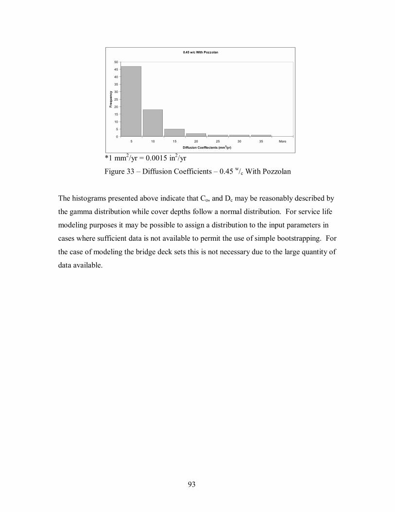
93

*1 mm2/yr = 0.0015 in2/yr

Figure 33 � Diffusion Coefficients � 0.45 w/c With Pozzolan

The histograms presented above indicate that Co, and Dc may be reasonably described by

the gamma distribution while cover depths follow a normal distribution. For service life

modeling purposes it may be possible to assign a distribution to the input parameters in

cases where sufficient data is not available to permit the use of simple bootstrapping. For

the case of modeling the bridge deck sets this is not necessary due to the large quantity of

data available.

0.45 w/c With Pozzolan

0

5

10

15

20

25

30

35

40

45

50

5 10 15 20 25 30 35 More

Diffusion Coeffiecients (mm2/yr)

Freq

uenc

y

94

ANALYSIS AND DISCUSSION

Validation of Service Life Model

The service life model that will be used for this project has been previously validated by

comparing the predicted service lives for a set of 129 bridge decks in Virginia to their

actual recorded service lives. (Kirkpatrick, 2001) To further validate the model the

predicted service lives for the 0.47 w/c bridge decks were compared to actual measured

deterioration levels. The 0.47 w/c bridge decks were investigated because they are the

oldest and reflect the most damage. The younger 0.45 w/c bridge decks have insufficient

damage to correlate the service life model to actual field conditions. Ten estimations of

the time to corrosion initiation were conducted using the actual field determined input

data presented in the previous section and the average time is presented in Table 12. The

individual data measurements were used in the corrosion initiation estimations as

opposed to the average values in order to incorporate the effects of input data variability.

Table 12 � Average Time to Corrosion Initiation (0.47 w/c Bare Steel Bridge Decks)

As shown the standard deviation is 1.5 years with a C.V. of 5.0 %. This level of

variability has been deemed acceptable for this application.

As determined previously using the Liu/Weyers and Vu, Stewart, and Mullard corrosion

propagation models the time to excessive concrete cracking is estimated to be 6 years for

bare steel bridge decks. Thus, the total time period for the 0.47 w/c set to reach a

deterioration level of 2% is 37 years.

From the damage surveys that were conducted on the 0.47 w/c bridge decks,

approximately 2% of the total area of the bridge deck set is currently showing signs of

corrosion damage (spalling, patches, or delaminations). The average age of the decks is

36.4 years with a range of 3 years and the predicted age of the set is 37 years. Thus, for

% Corroded

Average Time to Corrosion Initiation

(years)

Standard Deviation

(years) C.V. (%)2 30.7 1.5 5.0

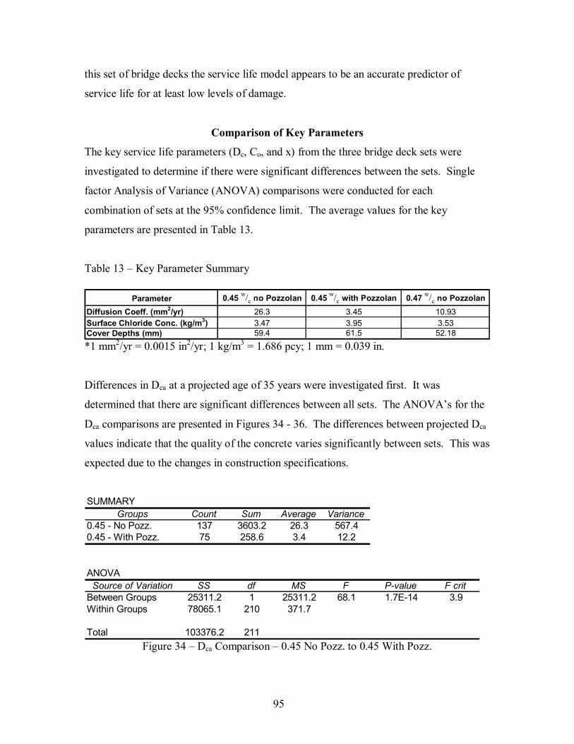
95

this set of bridge decks the service life model appears to be an accurate predictor of

service life for at least low levels of damage.

Comparison of Key Parameters

The key service life parameters (Dc, Co, and x) from the three bridge deck sets were

investigated to determine if there were significant differences between the sets. Single

factor Analysis of Variance (ANOVA) comparisons were conducted for each

combination of sets at the 95% confidence limit. The average values for the key

parameters are presented in Table 13.

Table 13 � Key Parameter Summary

*1 mm2/yr = 0.0015 in2/yr; 1 kg/m3 = 1.686 pcy; 1 mm = 0.039 in.

Differences in Dca at a projected age of 35 years were investigated first. It was

determined that there are significant differences between all sets. The ANOVA�s for the

Dca comparisons are presented in Figures 34 - 36. The differences between projected Dca

values indicate that the quality of the concrete varies significantly between sets. This was

expected due to the changes in construction specifications.

Figure 34 � Dca Comparison � 0.45 No Pozz. to 0.45 With Pozz.

Parameter 0.45 w/c no Pozzolan 0.45 w/c with Pozzolan 0.47 w/c no PozzolanDiffusion Coeff. (mm2/yr) 26.3 3.45 10.93Surface Chloride Conc. (kg/m3) 3.47 3.95 3.53Cover Depths (mm) 59.4 61.5 52.18

SUMMARYGroups Count Sum Average Variance

0.45 - No Pozz. 137 3603.2 26.3 567.40.45 - With Pozz. 75 258.6 3.4 12.2

ANOVASource of Variation SS df MS F P-value F crit

Between Groups 25311.2 1 25311.2 68.1 1.7E-14 3.9Within Groups 78065.1 210 371.7

Total 103376.2 211

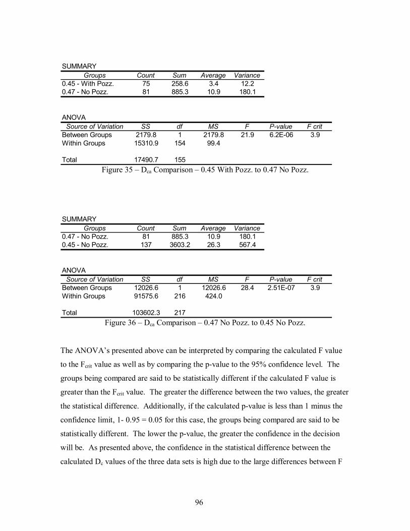
96

Figure 35 � Dca Comparison � 0.45 With Pozz. to 0.47 No Pozz.

Figure 36 � Dca Comparison � 0.47 No Pozz. to 0.45 No Pozz.

The ANOVA�s presented above can be interpreted by comparing the calculated F value

to the Fcrit value as well as by comparing the p-value to the 95% confidence level. The

groups being compared are said to be statistically different if the calculated F value is

greater than the Fcrit value. The greater the difference between the two values, the greater

the statistical difference. Additionally, if the calculated p-value is less than 1 minus the

confidence limit, 1- 0.95 = 0.05 for this case, the groups being compared are said to be

statistically different. The lower the p-value, the greater the confidence in the decision

will be. As presented above, the confidence in the statistical difference between the

calculated Dc values of the three data sets is high due to the large differences between F


0.47 - No Pozz. 81 885.3 10.9 180.10.45 - No Pozz. 137 3603.2 26.3 567.4



Total 103602.3 217


0.45 - With Pozz. 75 258.6 3.4 12.20.47 - No Pozz. 81 885.3 10.9 180.1



Total 17490.7 155

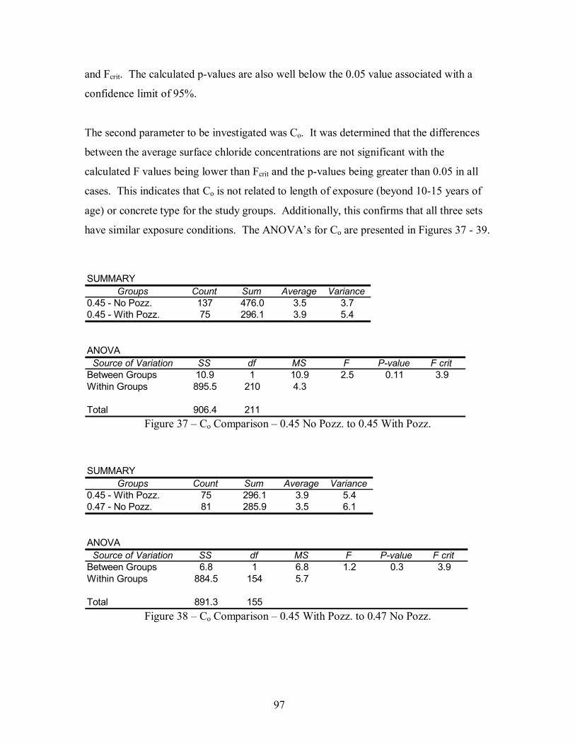
97

and Fcrit. The calculated p-values are also well below the 0.05 value associated with a

confidence limit of 95%.

The second parameter to be investigated was Co. It was determined that the differences

between the average surface chloride concentrations are not significant with the

calculated F values being lower than Fcrit and the p-values being greater than 0.05 in all

cases. This indicates that Co is not related to length of exposure (beyond 10-15 years of

age) or concrete type for the study groups. Additionally, this confirms that all three sets

have similar exposure conditions. The ANOVA�s for Co are presented in Figures 37 - 39.

Figure 37 � Co Comparison � 0.45 No Pozz. to 0.45 With Pozz.

Figure 38 � Co Comparison � 0.45 With Pozz. to 0.47 No Pozz.


0.45 - No Pozz. 137 476.0 3.5 3.70.45 - With Pozz. 75 296.1 3.9 5.4


Between Groups 10.9 1 10.9 2.5 0.11 3.9Within Groups 895.5 210 4.3

Total 906.4 211


0.45 - With Pozz. 75 296.1 3.9 5.40.47 - No Pozz. 81 285.9 3.5 6.1



Total 891.3 155

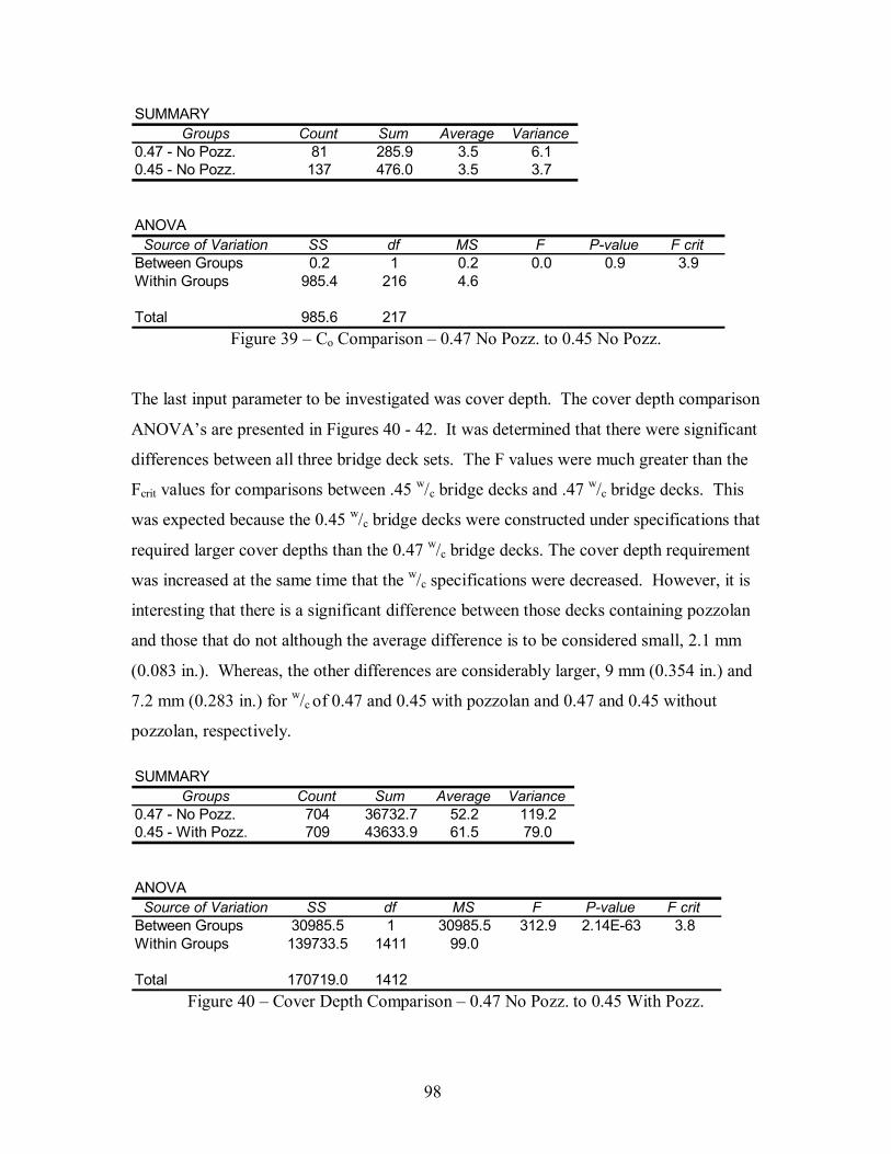
98

Figure 39 � Co Comparison � 0.47 No Pozz. to 0.45 No Pozz.

The last input parameter to be investigated was cover depth. The cover depth comparison

ANOVA�s are presented in Figures 40 - 42. It was determined that there were significant

differences between all three bridge deck sets. The F values were much greater than the

Fcrit values for comparisons between .45 w/c bridge decks and .47 w/c bridge decks. This

was expected because the 0.45 w/c bridge decks were constructed under specifications that

required larger cover depths than the 0.47 w/c bridge decks. The cover depth requirement

was increased at the same time that the w/c specifications were decreased. However, it is

interesting that there is a significant difference between those decks containing pozzolan

and those that do not although the average difference is to be considered small, 2.1 mm

(0.083 in.). Whereas, the other differences are considerably larger, 9 mm (0.354 in.) and

7.2 mm (0.283 in.) for w/c of 0.47 and 0.45 with pozzolan and 0.47 and 0.45 without

pozzolan, respectively.

Figure 40 � Cover Depth Comparison � 0.47 No Pozz. to 0.45 With Pozz.


0.47 - No Pozz. 81 285.9 3.5 6.10.45 - No Pozz. 137 476.0 3.5 3.7



Total 985.6 217


0.47 - No Pozz. 704 36732.7 52.2 119.20.45 - With Pozz. 709 43633.9 61.5 79.0



Total 170719.0 1412

99

Figure 41 � Cover Depth Comparison � 0.45 With Pozz. to 0.45 No Pozz.

Figure 42 � Cover Depth Comparison � 0.45 No Pozz. to 0.47 No Pozz.

Global Analysis

As stated previously the primary objective of this project is to model the service life of

the investigated bridge decks as three distinct sets: 0.47 w/c, 0.45 w/c, and 0.45 w/(c+p). It is

important to note that the 0.45 w/c bridge decks contain ECR, however, the effect of the

epoxy coating will be disregarded initially. This was done in order to investigate the

influence of the specification changes relating to increased cover depths, lowered w/c

ratios, and the addition of pozzolans. Additionally, although a statistical analysis of the

Co values indicated that there was no significant difference between sets, the Co values

from the 0.47 w/c bridge deck set were used during the analysis of all three sets to remove

any variability related chloride exposure.


0.45 - With Pozz. 709 43633.9 61.5 79.00.45 - No Pozz. 1291 76688.4 59.4 76.4



Total 156586.8 1999


0.45 - No Pozz. 1291 76688.4 59.4 76.40.47 - No Pozz. 704 36732.7 52.2 119.2



Total 206135.1 1994

100


The 0.47 w/c set was the first set to be analyzed and the results were used to validate the

service life model. The input data that was used for the service life model included 84 Co

measurements, 704 cover depth measurements, and 84 Dca values adjusted to an age of 35

years. The 22 years added to the time to 2% corrosion initiation is the result of 6 years to

corrosion cracking of 2% of the bridge deck plus 16 years for the damage to propogate

from 2% to 12%, the time at which an overlay is needed. The results of the service life

model are presented in Table 14.

Table 14 � Service Life Estimates � 0.47 w/c Bare Steel Bridge Decks

0.45 w/c and 0.45 w/(c+p) Bridge Decks

The same methodology was used to estimate the influence of the concrete quality used to

construct the 0.45 w/c bridge decks. By doing so, a direct comparison of concrete quality

between sets is possible. The data used in the service life model for concrete with and

without pozzolan was presented in Figures 28 - 30 previously. The total number of data

points used was as follows: No Pozzolan; Dca at 35 years � 114 values, Cover Depth �

1105 values; With Pozzolan; Dca at 35 years � 98 values, Cover Depth � 868 values.

The 84 surface chloride concentrations from the 0.47 w/c bridge decks were used as the

input for the 0.45 w/c decks in order to remove any environmental influence from the

analysis. Additionally, the Dca values that were calculated for the 0.45 w/c decks were

adjusted to reflect the time-dependency of the diffusion values as described previously.

The results of the service life model are presented in Table 15 for the 0.45 w/c bridge

decks.

Time (years)

St. Dev.(years) C. V. %

Time to 2 % Initiation 31 1.5 5.0Estimated Service Life 53 ----- -----

0.47 w/c no Pozzolan

101

Table 15 � Service Life Estimates - 0.45 w/c Bridge Decks

Comparison of 0.47 w/c and 0.45 w/c Bridge Decks

Analysis of the service life estimates at the 2% corrosion initiation level for the three

bridge deck sets demonstrated that the 0.45 w/c bridge decks with pozzolan were predicted

to be the most durable. The results demonstrate the influence of larger cover depths and

the lower Dca values associated with the 0.45 w/(c+p) set of bridge decks. More

importantly, however, is the lower predicted service life of the 0.45 w/c OPC bridge decks

as compared to the 0.47 w/c OPC bridge decks, 21 years and 31 years, respectively.

Although the predictions take into account the larger cover depths of the 0.45 w/c decks,

the larger Dca values have negated the influence of the larger cover depths. The higher

Dca values for the 0.45 OPC decks may be due to quality control/construction issues with

the newer 0.45 w/c OPC decks. It should be noted that the 10 - 0.47 w/c bridge decks used

in this study were selected from a previous study sample of which only 68% survived.

(Kirkpatrick, 2001) The bridges that had already been rehabilitated were removed from

the data set, as an accurate chloride analysis and damage survey would be impossible.

Therefore, the 10 decks selected were from the better performing 68%, which may place

some bias on the sample set.

The corrosion initiation period for 2% damage estimates illustrates that the addition of

pozzolan improves the long-term durability of bridge decks by decreasing the concrete

diffusivity. It appears that reducing the w/c of the concrete had a negligible effect. It can

be inferred that the study sample of the older 0.47 w/c concrete is of a higher quality than

the newer 0.45 w/c study sample.

Time (years)

St. Dev.(years) C. V. % Time (years)

St. Dev.(years) C. V. %

Time to 2 % Initiation 21 0.4 1.9 169 4.8 2.8Estimated Service Life 43 ----- ----- 191 ----- -----

0.45 w/c no Pozzolan 0.45 w/c with Pozzolan

102

Alternative Reinforcements

As discussed previously, alternative reinforcements can potentially increase the service

life of bridge decks substantially. In order to analyze the various alternatives, Dc, Co, and

cover depth values from the concrete containing pozzolans were used as input to the

service life model. These values were selected for use because they best represent the

current state of bridge deck construction in Virginia.

Epoxy-Coated Reinforcement

The corrosion initiation concentrations used for ECR were the same values that were

used for bare steel because research conducted by the FHWA concluded that �the

chloride threshold for damaged epoxy-coated bars is similar to that of black bars.�

(McDonald et al., 1998) Thus, areas of the epoxy coating that are damaged during

construction will initiate at the same chloride levels as bare steel and those areas will then

continue to propagate along the length of the reinforcing bar. However, there is evidence

that the corrosion propagation rate for ECR is lower than that of bare steel, which will

result in some additional service life for bridge decks containing ECR. (McDonald et al.,

1998; Brown, 2002)

Galvanized Steel

The chloride threshold values for galvanized steel are estimated to be 2.5 times greater

than carbon steel. (Yeomans, 2004) Corrosion initiation values were generated by simply

multiplying the bare steel initiation values by 2.5.

Stainless Steel

Chloride threshold values for stainless steel have been reported to be at least 10.4 times

greater than carbon steel. (Clemeña, 2003)

MMFX-2 Steel

Several research projects have attempted to estimate the chloride threshold value for

MMFX-2. The reported range of initiation values is 3.5 � 9.2 times that of carbon steel.

103

(Darwin et al, 2003; Trejo, 2002) A conservative initiation value of 3.5 times that of

carbon steel was used.

Service-Life Estimates

Using the adjusted chloride threshold values where appropriate, service-life estimates

were performed for the above reinforcement alternatives. The estimates should provide a

reasonable expectation of the time required for corrosion to initiate. It should also be

noted that alternative reinforcements will have longer corrosion propagation times, which

are not included in the service-life estimates presented below. (See Table 16)

Table 16 � Service Life Predictions (Alternative Reinforcements) � A4 Concrete - w/c =

0.45 with pozzolan

As shown, bridge decks constructed using current bridge deck specifications (0.45 w/c

with pozzolan and 2 in. minimum cover depths) will in most cases never initiate

corrosion within the desired service life of 100 years regardless of reinforcement type.

Galvanized, stainless steel, and MMFX-2 reinforcement will provide a reliable second,

redundant corrosion protection system where such systems are required.

Individual Deck Analysis

After validating the service life model and comparing the service life estimates of the

three bridge deck sets the potential for the model to estimate the service life of an

individual deck was investigated. The data collected for each individual bridge deck was

used as input to the service life model and the results compared to actual field conditions.

The input generally consisted of 9 Co values, 9 Dca values, and 40-80 cover depth, x

values. The number of values for Co and Dca was lower in some instances due to missing

or inconsistent data and the number of cover depth measurements was dependent upon

the length of the deck.

Reinforcement Type Bare Epoxy-Coated Galvanized Stainless MMFX-2Time to 2 % Initiation 160 160 602 9999 1312

Time to Initiation (years)

104

The ability of the service life model to accurately estimate the service lives of individual

bridge decks was first investigated using the 0.47 w/c bridge deck data. The service life

estimates for those ten bridge decks are presented in Table 17.

Table 17 � 0.47 w/c Bridge Deck Service Life Estimates - Individual

As is evident in Table 17, the model is not capable of accurately estimating the service

life for individual bridge decks on a consistent basis with the amount of data available.

The model overestimates the service life in some cases and underestimates in others. It is

believed that the models� inability to accurately predict the service lives of individual

bridge decks is related to the quantity of input data. Low quantities of input data may not

accurately represent the characteristics of the bridge decks. The parameter where this is

most evident is Dca. It is possible for an individual bridge deck to have a coefficient of

variation in excess of 100% for Dca. Therefore, the probability of 9 values being able to

accurately define the distribution is low. Due to the observed inability of the model to

predict the service lives of the 10 bridge decks investigated, any analysis of individual

bridge decks should be viewed with caution. The required amount of input data is

currently unclear. It may be possible, however, to determine the probability of corrosion

initiating based upon a limited number of diffusion parameters measured in the field.

The estimated times for 2% corrosion initiation for all of the bridge decks are presented

in Table 18. As mentioned previously, due to the limited amount of input data available,

these estimations should be viewed with caution.

Structure # % DamageTime to Initiation 2% or less (years)

Time to Corrosion Cracking

Propagation Time (years)

Estimated Age(years)

Actual Age(years)

Difference(years)

1-1804 5.3 13 6 6 25 37 121-6101 0.0 > 100 6 --- --- 37 ---2-2007 2.3 18 6 1 25 36 113-1021 0.2 11 6 --- 17 35 184-1062 0.0 > 100 6 --- --- 37 ---4-2049 0.7 > 100 6 --- 100 38 -625-1800 3.3 > 100 6 3 100 36 -646-1032 0.0 > 100 6 --- --- 35 ---9-2801 3.0 72 6 2 80 36 -449-6042 1.1 32 6 --- 38 37 -1

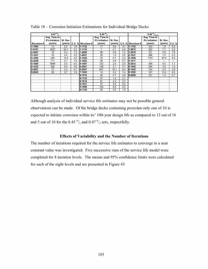
105

Table 18 � Corrosion Initiation Estimations for Individual Bridge Decks

Although analysis of individual service life estimates may not be possible general

observations can be made. Of the bridge decks containing pozzolan only one of 10 is

expected to initiate corrosion within its� 100-year design life as compared to 12 out of 16

and 5 out of 10 for the 0.45 w/c and 0.47 w/c sets, respectfully.

Effects of Variability and the Number of Iterations

The number of iterations required for the service life estimates to converge to a near

constant value was investigated. Five successive runs of the service life model were

completed for 8 iteration levels. The means and 95% confidence limits were calculated

for each of the eight levels and are presented in Figure 43.

Structure #

Avg. Time to 2% Initiation

(years)St. Dev.(years) C.V. % Structure #


(years)St. Dev.(years) C.V. % Structure #


(years)St. Dev.(years) C.V. %

1-1804 13 0.2 1.8 1-1132 17 0.6 3.7 1-1152 333 1.8 0.51-6101 2027 64.7 3.2 1-1133 7 0.1 2.0 1-2815 252 7.7 3.02-2007 18 0.3 1.5 1-2820 66 0.8 1.2 1-2819 63 4.9 7.83-1021 16 0.5 3.2 1-6051 28 1.0 3.5 2-1021 286 1.0 0.34-1062 325 14.5 4.5 2-1020 32 0.7 2.3 3-1000 1181 97.5 8.34-2049 111 2.1 1.9 3-1003 28 0.8 2.7 3-1017 --- --- ---5-1800 9999 0.0 0.0 4-1007 123 2.4 2.0 5-2812 399 4.4 1.16-1032 260 9.4 3.6 4-2901 138 5.1 3.7 8-1002 259 3.9 1.59-2801 72 3.4 4.7 5-2547 847 76.1 9.0 8-1042 144 4.0 2.89-6042 36 0.7 1.8 7-1920 14 0.2 1.4 9-1002 161 10.4 6.4

8-1019 26 0.7 2.8 9-6058 191 1.4 0.78-1133 47 1.4 3.19-1014 61 2.3 3.79-1031 27 0.6 2.49-1098 154 6.6 4.39-1139 28 0.5 1.8

0.45 w/(c+p)0.45 w/c0.47 w/c

106

Figure 43 � Iteration Analysis for 0.47 w/c Bridge Deck Set

As shown, 95% confidence intervals range from a maximum of +/- 7.8 years for 500

iterations to a minimum of +/- 0.8 years for 64000 iterations. The service life model is

currently capable of 65000 iterations, which yields a 95% confidence interval of less than

+/- 0.8 years. That level of variability has been deemed acceptable for bridge deck

service life estimates and was the number of iterations used in all of the previously

presented analyses.

It is important to note that the precision of the model is not at all related to the accuracy

of the service life estimations. While the model has a 95% confidence interval of +/- 0.8

years the accuracy of service life estimations remains dependent upon the accuracy and

quantity of the input data as well as the models� ability to accurately estimate the

mechanisms of deterioration. Service life estimations are sensitive to variations in the

input data, so it is pertinent that great care be taken with field and laboratory data

collection. The sensitivity of each individual input parameter is investigated in the

following section.

20.00 25.00 30.00 35.00 40.00 45.00Time to 2% Initiation (years)

500 Iterations

1000 Iterations

2000 Iterations

4000 Iterations

8000 Iterations

16000 Iterations

32000 Iterations

64000 Iterations

107

Sensitivity Analysis

The effect of the sensitivity of the input variables on the estimated time to corrosion

initiation was investigated. Understanding the sensitivity of the input parameters is

important for identifying possible sources of error and variability in the service life

estimations. The more sensitive that an input parameter is to the estimation the more

important it is to determine accurate values for that parameter.

Apparent Diffusion Coefficient (Dca)

The relationship between Dca and time to corrosion initiation is presented in Figure 44.

*1 mm2/yr = 0.0015 in2/yr Figure 44 � Apparent Diffusion Coefficient vs. Time to Corrosion Initiation

The relationship becomes asymptotic for both high and low values of Dca. As shown, the

changes in the time to corrosion initiation are relatively small for Dca values greater than

40 mm2/yr (0.06 in2/yr). However, for small changes in Dca less than 10, the increase in

time to initiation can be large, doubling from 80 to 160 years from 10 to 5 mm2/yr

(0.0075 in2/yr) for example. Variations in Dca values from 10 and 40 mm2/yr (0.015 and

0

10

20

30

40

50

60

70

80

90

100

0 20 40 60 80 100 120 140 160 180 200

Time to Corrosion Initiation (years)

Dc (

mm

2 /yr)

Co = 2.5 Co = 3.5 Co = 4.5 Co = 5.5

x = 60 mmCx,t = 0.7 kg/m3

108

0.06 in2/yr) will yield relatively large changes in the estimated time to corrosion

initiation, generally about 60 years. These relationships are generally valid for all four

concentrations of Co presented and as expected lower levels of Co will result in longer

times to corrosion initiation. However, the additional time to corrosion initiation that can

be attributed to lower levels of Co is relatively small in comparison to the effect of Dca.

As presented in the previous Diffusion Coefficient section the average Dca values for the

sampled bridge decks are generally in the range of 1 � 40 mm2/yr (0.0015 � 0.06 in2/yr).

The sensitivity analysis indicates that Dca values within this range are highly sensitive,

which gives reason for some concern. Dca values are the most difficult input parameter to

obtain and are generally the most variable. For that reason it is recommended that Dca be

determined from field data whenever possible as opposed to using experimental results to

set values for Dca. The sensitivity analysis also reinforces the importance of using a

range of Dca values rather an average value, as Dca can vary significantly within an

individual bridge deck.

Surface Chloride Concentration (Co)

The relationship between Co and the time to corrosion initiation is presented in Figure 45.

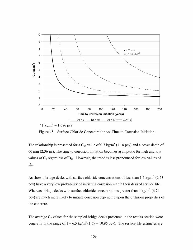
109

*1 kg/m3 = 1.686 pcy

Figure 45 � Surface Chloride Concentration vs. Time to Corrosion Initiation

The relationship is presented for a Cx,t value of 0.7 kg/m3 (1.18 pcy) and a cover depth of

60 mm (2.36 in.). The time to corrosion initiation becomes asymptotic for high and low

values of Co regardless of Dca. However, the trend is less pronounced for low values of

Dca.

As shown, bridge decks with surface chloride concentrations of less than 1.5 kg/m3 (2.53

pcy) have a very low probability of initiating corrosion within their desired service life.

Whereas, bridge decks with surface chloride concentrations greater than 4 kg/m3 (6.74

pcy) are much more likely to initiate corrosion depending upon the diffusion properties of

the concrete.

The average Co values for the sampled bridge decks presented in the results section were

generally in the range of 1 � 6.5 kg/m3 (1.69 � 10.96 pcy). The service life estimates are

0

1

2

3

4

5

6

7

8

9

10

0 20 40 60 80 100 120 140 160 180 200


Co (

kg/m

3 )

Dc = 5 Dc = 10 Dc = 20 Dc = 40

x = 60 mmCx,t = 0.7 kg/m3

110

fairly sensitive to Co values within this range for bridge decks with Dca values greater

than 20 mm2/year (0.03 in2/yr). However, for bridge decks with Dca values less than 10

mm2/yr (0.015 in2/yr) the magnitude of Co is irrelevant because of the large estimated

time to initiation values.

Cover Depth (x)

The relationship between cover depth and time to corrosion initiation is presented in

Figure 46.

*1 mm = 0.039 in.

Figure 46 � Cover Depth vs. Time to Corrosion Initiation

For cover depths greater than 35 mm (1.38 in.) it is reasonable to model the relationship

between cover depth and time to corrosion initation using a linear function. The slope of

the line is dependent upon the associated diffusion coefficient. As shown, the cover

depth is the least sensitive input parameter of the three. The cover depth is also the input

parameter with the least variability.

35

40

45

50

55

60

65

70

75

0 20 40 60 80 100 120 140 160 180 200


Cov

er D

epth

(mm

)

Dc = 5 Dc = 10 Dc = 20 Dc = 40

Co = 3.5 kg/m3

Cx,t = 0.7 kg/m3

111

The effect of cover depth variability on the service life estimations of bridge decks

constructed with low permeable concrete (Dca < 10 mm2/yr [0.015in2/yr]) is irrelevant

because in most instances corrosion will not initiate within a 100 year design life.

However, for bridge decks with highly permeable concrete (Dca > 20 mm2/yr [0.03

in2/yr]) the effect is more significant.

112

LIFE CYCLE COST ANALYSIS (LCCA)

The total cost of a bridge deck cannot be described by a one-time construction

expenditure. There are always agency costs related to the operation, maintenance, repair

and rehabilitation of a bridge deck throughout its� service life. Often times there are

many alternatives available for maintaining a bridge deck, with different costs and

timings associated with each. Due to the variety of bridge management options available

it has become necessary to analyze the alternatives and select the most economical

option. This, however, is not as simple as summing the expected costs for each

alternative. The time-value of money and the affect on the user must also be considered.

To assist in the comparison of alternatives an approach referred to as Life-Cycle Cost

Analysis (LCCA) is commonly used. LCCA is a methodology that has received much

attention in recent years as a means of comparing available management alternatives.

LCCA as related to bridges can be defined as �a set of economic principles and

computational procedures for comparing initial and future costs to arrive at the most

economical strategy for ensuring that a bridge will provide the services for which it was

intended.� (Hawk, 2003)

LCCA may be separated into the five basic steps listed below:

1. Establish design alternatives

2. Determine activity timing

3. Estimate costs (agency and user)

4. Compute life-cycle costs

5. Analyze the results (FHWA, 2002)

Step 1: Establishing Design Alternatives

The first step in conducting a LCCA is to define the possible design/maintenance

alternatives. To begin with, there is the possibility of having multiple initial construction

options. Each construction option will have an associated maintenance expectation.

Secondly, the different maintenance strategies must be identified. When establishing the

design alternatives to be compared it is best to vary only one parameter at a time. For

example if different initial construction options are being compared, the maintenance

113

strategy selected should be the same for both. However, the implementation times of the

individual maintenance activities will most likely be different for comparison design

alternatives. Otherwise, it may not be possible to identify what parameter is contributing

to the lower cost, initial construction or maintenance strategy. After a construction

option is selected the possible maintenance alternatives can then be investigated.

Step 2: Determine Activity Timing

Once the possible design alternatives have been identified the timing of the

maintenance/repair activities must be determined. Different maintenance/repair activities

will extend the service life of a bridge deck by varying degrees. Therefore, the timing of

subsequent repairs will be affected by the initial maintenance strategy selected. For

example, a latex concrete overlay may extend the service life of a bridge deck by 25

years whereas a polymer overlay may only extend the service life by 15 years after which

time additional repair/rehabilitation measures must be taken. Determining the

appropriate timing of the design alternatives is important in that it will affect the total

amount of maintenance that will be projected for an alternative within the analysis time

period. Additionally, the time value of money plays a large role in LCCA, so if the

selected timings are not accurate the resulting life cycle cost estimations may not be

reliable.

One important aspect of LCCA is that all design/maintenance alternatives must be

compared using a common service life period. Thus, the desired service life of a

structure must be predetermined and any remaining service life provided by a

maintenance alternative after the end of the analysis period will not be considered. The

remaining service life may be accounted for by assigning a positive salvage value at the

end of the analysis. However, this may not be desirable as a predetermined service life

may indicate that the structure is expected to be functionally obsolete at that time and

would require replacement regardless of the state of deterioration. Therefore, any

remaining service life would be irrelevant.

114

Step 3: Estimate Costs (Agency and User)

The costs that are necessary to conduct a LCCA are all the costs associated with each

design alternative that are not common to all alternatives. For example the costs of

different overlays must be provided, but the costs of biannual inspections do not because

they are required for all alternatives regardless of overlay type. The costs that are

required include not only those related to the actual construction/repair (Agency Costs),

but also the costs related to the impact on the user (User Costs).

Agency Costs

Agency costs are those costs associated with the design, initial construction, maintenance

(preventative and corrective), rehabilitation, and replacement of a structure. They will

also include costs incurred that are related to traffic control and mobilization. Agency

costs are in general much easier to estimate than user costs. Estimates can be made for a

particular activity based upon historical bid records and engineering judgement.

The salvage value of a structure is another agency cost that may be considered. It is

defined as the value of any alternative at the end of the analyis period. The salvage value

may be positive for alternatives with a remaining service life or if the structure/element

has some residual value or it may be negative in instances where there is a cost associated

with the removal and disposal of material.

User Costs

For a LCCA to be complete the indirect costs incurred by the public (users) for each

alternative must be considered. These costs �typically arise from the timing, duration,

scope, and number of construction and rehabilitation work zones characterizing each

project alternative.� (FHWA, 2002) The user costs associated with transportation projects

can generally be separated into three categories: Vehicle Delay Costs, Vehicle Operating

Costs, and Accident Costs. The three user cost categories can be defined as follows:

1. Vehicle Delay Costs - the personal cost to drivers delayed by roadwork;

115

2. Vehicle Operating Costs - the costs associated with the operation of vehicles delayed

by roadwork; and

3. Accident Costs - the cost of damage to vehicles and injury to people due to roadwork.

The following formulas have been developed to estimate the user costs associated with a

given construction alternative.

�Equation 33 can be used to compute the cost to drivers of roadwork-related traffic

delays.

wNADTSL

SLayCostsVehicleDel

na

×××

−= Equation 33

where:

L is the length of affected roadway or which cars drive,

Sa is the traffic speed during bridge work activity,

Sn is the normal traffic speed,

ADT is the average daily traffic, measured in number of cars per day,

N is the number of days of road work, and

w is the dollar value of each hour of a driver�s time.

The hourly value w is a weighted average of commercial vehicle drivers� and personal

automobile drivers� time.

Vehicle operating costs can be calculated using Equation 34.

rNADTSL

SLsratingCostVehicleOpe

na

×××

−= Equation 34

where r is a weighted-average vehicle cost similar to the weighted cost in Equation 33

and the remaining parameters are the same as those in Equation 33.

116

Accident costs can be calculated using Equation 35.

( ) ana cAANADTLstsAccidentCo ×−×××= Equation 35

where ca is the cost per accident, Aa and An are the during-construction and normal

accident rates per vehicle-kilometer, and the remaining parameters are the same as those

listed in Equations 33 and 34.� (Ehlen, 2003)

Step 4: Compute Life-Cycle Costs

Once the design alternatives have been defined and their associated activity timings and

costs determined their LCC�s may be calculated. LCC comparisons are based upon the

economic principle that there is a time-value of money. Thus, depending upon the

discount rates and inflation rates the value of one dollar now will be higher or lower in

the future. The concept of the time-value of money is discussed in more detail in the

following section. The importance of this concept is to realize that the anticipated cost of

future repairs cannot be simply added together to determine the LCC for a specific design

alternative.

In order to conduct a LCCA a base year for comparison must be selected. Generally, the

current year is selected to allow for the use of simple present worth computations and

current cost data. The equation that is used to calculate the present worth of a single

future expenditure is presented below.

( )nrFVPW+

=1

Equation 36

where:

PW = Present Worth

FV = Future Value

117

r = Real discount rate (Nominal discount rate � Inflation)

n = Number of years in the future that the cost will be incurred

In some cases it may be desirable to model future expenditures as either a uniform cost

over a given number of years or as a gradient series. A gradient series would be used for

expenditures that increase year-over-year. For example, as a bridge deck begins to

deteriorate it will require more patching in year 5 than in year one. Therefore, a gradient

series may be used to model that increase in maintenance costs. A uniform series would

be used in cases where the expenditure is expected to remain constant for a set time

period. For example, a bridge deck may require annual maintenance throughout its

service life. Equations 37 and 38 are used to convert these expenditures to a present-

worth value.

( )( )n

n

rrrPWUS+

−+=1

11 Equation 37

( )( )

−−+×

+= n

rr

rrPWGS

n

n

111

1 Equation 38

where:

PWUS = Present Worth of a Uniform Series

PWGS = Present Worth of a Gradient Series

Typically, a single cost, uniform series, or a gradient series will occur at some specified

point in the future. To convert the present worth of a single expenditure calculated for a

uniform or gradient series to the present worth in the base year Equation 36 is used.

Time-value of Money

As mentioned previously, LCCA is based upon the concept that money has a time-value.

The basis of time-value lies in the idea that money not spent today can be placed into an

investment vehicle, which will provide some return over time. For example, if $100 were

118

placed into an investment account that provides an interest rate of 5% per year, one year

later that account would be worth $105. Therefore, $105 one year from now would have

an equivalent value of $100 today, in this example. To account for the time-value of

money discount rates and inflation rates are used.

Discount Rate

The discount rate �is a parameter used to calculate the equivalent worth of economic

resources used or received now or in the future.� (Hawk, 2003) The discount rate can be

given as the nominal discount rate (the discount rate including inflation), or the real

discount rate (the discount rate less inflation). LCC comparisons use real discount rates.

By doing so, the opportunity value of money is incorporated into the analysis.

The applicability of discount rates to public agency cost analyses is debatable. The

problem with applying discount rates to transportation projects arises in the fact that

transportation officials do not typically have the option of investing money saved in the

present for use in the future. Therefore, there would be no potential return on investment.

However, it is possible that money saved initially may be invested in other projects that

will yield some tangible benefit, as in extended service life of a structure or beneficial

research. Discount rates as high as those evident in the private sector are not expected,

however, some opportunity value of money should be considered. Currently, government

agencies are instructed to use guidelines provided by the Office of Management and

Budget (OMB). The discount rate that is specified for use in cost analyses is the real

discount rate that corresponds to the interest rate on the treasury note or bond that has the

same maturity time as the analysis time period being investigated. For example, a project

that has an analysis time period of 10 years should be investigated using the real discount

rate that corresponds to the 10-year treasury note. Interest rates for treasury notes and

bonds are updated annually and can be found in Appendix C of Circular No. A-94. This

information can be easily located at the OMB website www.whitehouse.gov/omb/. The

following rates are current as of January 2007: (OMB, 2007)

119

Table 19 � Nominal and Real Interest Rates on Treasury Notes and Bonds

Nominal Interest Rates on Treasury Notes and Bonds of Specified Maturities (in percent)

3-Year 4.9

5-Year 4.9

7-Year 4.9

10-Year 5.0

20-Year 5.1

30-Year 5.1

Real Interest Rates on Treasury Notes and Bonds of Specified Maturities (in percent)

3-Year 2.5

5-Year 2.6

7-Year 2.7

10-Year 2.8

20-Year 3.0

30-Year 3.0

For the analysis of bridge decks the specified service life is generally either 75 or 100

years. Therefore, the real interest rate of the 30-year treasury note should be used in their

LCCA�s. It should be noted that predicting interest rates and inflation rates at distant

points in the future should be done with caution. There is a high level of uncertainty

associated with these estimations.

Inflation/Deflation Rate

Inflation can be defined as a rise in the general level of prices, as measured against some

baseline of purchasing power. Inflation affects LCCA in that the cost of materials and

construction will increase over time. Conversely, if deflation occurs costs will be lower

in the future. Historically, the United States economy has been subject to inflation with

only several short periods of price deflation. The inflation rate can be estimated using

many different indexes ranging from those that track broad-based consumerism to those

that monitor only a niche market. The index that is most commonly used to determine

inflation rates in the United States is the Consumer Price Index (CPI). It may be

reasonable to apply inflation rates determined from the CPI to the inflation rate of

construction materials; however, given that there are indexes available that specifically

track the inflation of construction materials and labor the CPI may not be the most

120

applicable for LCCA of bridge decks. Three indexes that relate specifically to

construction were investigated in this study: Engineering News Record Construction

Cost Index, FHWA Composite Construction Cost Index, and FHWA Structures

Construction Cost Index. These cost indexes and and their associated inflation trends

will be discussed in detail in the �LCCA�s of Virginia Bridge Decks� section.

Deterministic vs. Probabilistic

LCCA�s can be conducted using deterministic or probabilistic input parameters. A

deterministic analysis requires a specific application time for each expenditure.

Conversely, a probabilistic analysis enables the user to assign a probability distribution to

input parameters. An example of a deterministic analysis would be a bridge deck

requiring an overlay at 50 years of age. In reality there is some uncertainty associated

with the timing of specific maintenance events. Therefore, it is more appropriate to

specify an overlay installation at times normally distributed around a mean of 50 years.

This procedure may be completed for each maintenance, repair, and rehabilitation event

for each alternative. The LCCA program will then randomly select timings for each

event according to their distributions and compute an associated LCC. The selection

process is repeated many times and a distribution of present values as well as a mean

value will be generated. The generated present value distributions can then be compared

for each alternative.

The problem that arises when incorporating the probabilistic nature of input parameters is

being able to accurately define the distributions for those parameters. Large amounts of

data are typically required to define distributions for a specific event. Therefore, a

probabilistic analysis may not be appropriate in all cases.

Step 5: Analyze the Results

Analyzing the results of a LCCA can be straightforward or quite complex depending

upon the method of analysis used. If a deterministic approach is used, analyzing the

results may be as simple as comparing the computed present values of each alternative.

However, if a probabilistic approach is used additional consideration must be given to the

121

results. In a probabilistic analysis the selection of multiple alternatives is possible

depending upon the level of risk that the user is willing to accept.

Often times it is also desirable to perform a sensistivity analysis on the LCCA.

Sensitivity analyses are performed by varying the timings of expenditures and discount

rates within a LCCA to determine how sensitive the analysis is to specific parameters. If

an analysis is found to be highly sensitive to an individual parameter it may be necessary

to better define the input data for that variable.

The user may also choose not to consider user costs in the analysis, as they may not be

confident in their validity or may simply not be concerned with their effects. Finally, the

user should reevaluate the possible design alternatives to determine if modifications can

be made to provide a more cost effective approach. Reevaluations, commonly known as

concurrent engineering, are necessary if either the agency costs or user costs are found to

be disproportionately high for a specific alternative.

LCCA�s of Virginia Bridge Decks

LCCA�s for bridge decks constructed under current design specifications are unnecessary

because as demonstrated previously the estimated service life of 0.45 w/c+p bridge decks

will exceed a specified design life of 100 years regardless of reinforcement type.

Therefore, reinforcement type should be selected solely on a first-cost basis except in

cases where extreme chloride exposure is expected.

However, the question remains as to what the best maintenance strategy is for bridge

decks constructed under previous specifications. Therefore, multiple maintenance

alternatives will be analyzed to determine the optimum maintenance strategy for in-place

bridge decks. The LCCA�s will be conducted according to the methodology presented

previously for a design life of 100 years and a base year of 2008. A base year of 2008

was selected because it is anticipated that 2008 will be the earliest possible time of

implemenation for this project. LCC comparisons in the examples presented will be

122

based upon computed unit costs ($/SY; $/m2). Using the calculated unit costs, LCC�s for

bridge decks of any size can be easily computed relative to their surface areas.

Step 1: Establish Design Alternatives

Bridge deck LCCA�s will be conducted for two possible repair/rehabilitation alternatives

for preventing/repairing corrosion related deterioration. The initial condition of the

bridge decks to be compared will be considered equivalent. Therefore, the only

differences in the LCCA alternatives are related to the maintenance procedures. The two

deck maintenance alternatives that will be investigated are polymer overlays and concrete

overlays (microsilica/latex-modified).

Maintenance Alternative 1: Polymer Overlays

The first maintenance alternative to be investigatied is the use of polymer overlays as a

preventative maintenance technique. Polymer overlays are used primarily to reduce the

rate of ingress of water and chlorides into the concrete as well as to improve skid

resistance, ride quality, and surface appearance. (Krauss and Ferroni, 1986; Sprinkel,

1989) They are to be installed prior to extensive corrosion related deterioration. Polymer

overlays are suitable for bridge decks that reflect between 0-1% corrosion related

deterioration in the worst span lane. Bridge decks that have corrosion-deteriorated areas

in excess of 1% should be repaired/rehabilitated using alternative maintenance strategies.

Polymer overlays are not recommended for use on bridge decks that have any of the

following characteristics:

1. �Corrosion-induced delamination and spalls

2. Cover concrete that is critically chloride-contaminated

3. Half-cell potentials more negative than �250 mV CSE

4. Unsound concrete (tensile rupture strength less than 150 psi)

5. Poor drainage

6. Poor ride quality� (Weyers et al, 1993)

If the bridge deck being investigated reflects any of the above characteristics the use of a

concrete overlay may be more appropriate.

123

The estimated service life of a polymer overlay ranges from 10 years for a bridge with a

very high ADT (> 50,000) to 25 years for a bridge with a low to moderate ADT (< 5000).

(Weyers et al, 1993) For purposes of this analysis polymer overlays will be investigated

for service lives of 10, 15, and 25 years. In addition to the cost of the overlay the cost

associated with 1% patching of the bridge deck at the time of the overlay will be taken

into account. For an individual bridge deck it may be necessary to place multiple

overlays in order to reach the desired service life. When that is the case the installation of

the polymer overlay will become a recurring cost as well as the removal of preceding

overlays.

Maintenance Alternative 2: Concrete Overlays

The second maintenance alternative that will be investigated is the use of concrete

overlays as a deck rehabilitation measure. They are used as a repair/rehabilitation

method for decks reflecting significant levels of corrosion related deterioration. The

installation of concrete overlays requires that a specified depth of the cover concrete be

removed by milling and the underlying concrete removed and patched as necessary. In

order to provide the desired service life �all spalled, delaminated, actively corroding, and

critically chloride-contaminated concrete� must be removed and repaired prior to

placement of the overlay. (Weyers et al, 1993)

Concrete overlays are typically used as a rehabilitation method for bridge decks that have

reached their EFSL. As mentioned previously the EFSL for a bridge deck is defined in

this project as the time at which 12% of the bridge deck has deteriorated in the worst span

lane. Therefore, a maintenance strategy that specifies the use of a concrete overlay must

consider the costs associated with 12% patching of the bridge deck prior to placement of

the overlay. As demonstrated by this project the required patching will occur on average

during the 16 years preceding the placement of the overlay.

The service life of a concrete overlay is estimated to be between 22 and 26 years and is

dependent upon the severity of chloride exposure and condition of the underlying

124

concrete, but is independent of ADT. (Weyers et al, 1993) The overlay service life used

in the following analyses is 25 years. The cost for 12% patching, milling, and groving of

the bridge deck for each required overlay is also included.

Step 2: Determine Activity Timing

With the two maintenance alternatives identified the next step is to determine the timings

of the associated maintenance activities. The activity timings presented in Table 20

represent those timings associated with a bridge deck that has a current deterioration level

between 0 and 1%. Year zero does not represent the the time at which the bridge deck is

put in place but rather the time of analysis.

Table 20 � LCCA Maintenance Activity Timing

As shown, a bridge deck with 0 - 1% corrosion related damage would either require a

polymer overlay in the current year or a concrete overlay approximately 15 years in the

Year VH H M0 PO & 1% P PO & 1% P PO & 1% P5 6% P10 OR, PO, & 1% P 6% P15 OR, PO, & 1% P M, CO, & G20 OR, PO, and 1%P25 OR, PO, & 1% P30 OR, PO, and 1%P OR, PO, & 1% P 6% P35 6% P40 OR, PO, and 1%P M, CO, & G45 OR, PO, & 1% P50 OR, PO, and 1%P OR, PO, & 1% P55 6% P60 OR, PO, and 1%P OR, PO, & 1% P 6% P65 M, CO, & G70 OR, PO, and 1%P75 OR, PO, & 1% P OR, PO, & 1% P80 OR, PO, and 1%P 6% P85 6% P90 OR, PO, and 1%P OR, PO, & 1% P M, CO, & G95

100* PO = Polymer Overlay; P = Patching; OR = Overlay Removal; M = Milling; CO = Concrete Overlay; G = Bridge Deck Grooving

Polymer OverlaysADT Concrete Overlays

125

future. For the case of a polymer overlay, the 0 � 1% of deteriorated deck would be

patched at the time of the overlay. Additionally, for subsequent polymer overlays there is

a cost associated with the removal of the previous overlay. Concrete overlays are not

placed until substantial deterioration is evident (12% of the worst span lane). The

maintenance activity timings presented reflect the 12% of required patching prior to

placement of the concrete overlay. For simplicity the patching has been estimated to

occur in equal amounts of 6% at 5 and 10 years prior to the placement of the concrete

overlay. The required milling and bridge deck grooving associated with a concrete

overlay are also considered.

It should be noted that the activity timings presented in Table 20 are only valid for bridge

deck maintenance decisions made in the current year (2008). For bridge decks that do

not currently require maintenance, activity-timing tables must be developed for future

years. LCC comparison tables will be developed and presented for the maintenance

alternatives where strategy decisions are to be made in the year 2008, 2018, 2028, 2038,

2048, and 2058.

It is important to note that the maintenance timings presented may be altered at the

discretion of the engineer. The estimated service lives of the overlays are intended to

reflect the average expected service life for a given set of circumstances. The actual

service life of an overlay is dependent upon the severity of the environment to which it is

exposed, the condition of the underlying deck, the quality of construction, and the level

of traffic on the bridge. The purpose of the examples provided in this report is to present

the concepts of LCCA rather than to make determinations for the maintenance strategies

of individual bridge decks.

Step 3: Estimate Costs

The next step in conducting the LCCA is to determine the costs associated with each

maintenance alternative. As mentioned previously, the base year for comparison is 2008.

Therefore, all maintenance expenditures presented in this section will be adjusted to

reflect their estimated costs in 2008. The costs will be estimated using tabulated VDOT

126

bid data from 1997, 1999, and 2004. The average inflation rate will be determined for

each bid item for the time period of 1997 � 2004. Using the 2004 cost data and the

average inflation rate the costs will then be projected for the year 2008. The bid items

associated with the two maintenance alternatives are presented below:

Alternative 1 � Polymer Overlays

• Patching � Type B � The removal and patching of deteriorated concrete to a depth

below the first mat of reinforcement.

• Polymer Overlay � The placement of a multi-layer polymer overlay on the entire

bridge deck.

• Polymer Overlay Removal � The removal of a previous polymer overlay prior to

the placement of a subsequent overlay.

• Traffic Control � The cost associated with controlling the traffic over the lifetime

of the project.

• User Costs � Costs incurred by the traveling public attributable to the construction

project. Varies between projects and therefore will not be considered in the

presented examples.

Alternative 2 � MSC/LMC Overlays

• Patching � Type B

• Milling Type A � The removal of the top ½ in. of concrete prior to placement of a

concrete overlay.

• Concrete Overlay � The placement of a concrete overlay with a specified depth of

1 ¼ in. � 1 ¾ in.

• Bridge Deck Grooving � The grooving of the concrete overlay after placement

and curing.

• Traffic Control

• User Costs � Again, because user costs are site specific, they are not included in

the presented examples.

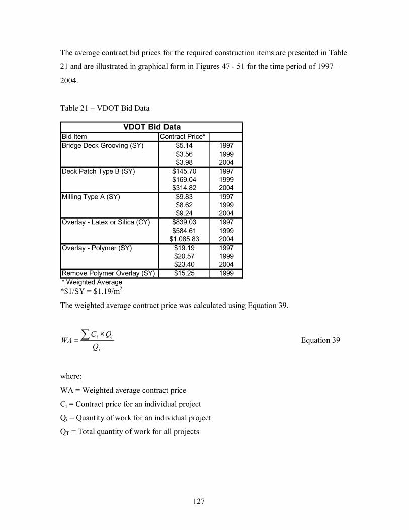
127

The average contract bid prices for the required construction items are presented in Table

21 and are illustrated in graphical form in Figures 47 - 51 for the time period of 1997 �

2004.

Table 21 � VDOT Bid Data

*$1/SY = $1.19/m2

The weighted average contract price was calculated using Equation 39.

T

ii

QQC

WA ∑ ×= Equation 39

where:

WA = Weighted average contract price

Ci = Contract price for an individual project

Qi = Quantity of work for an individual project

QT = Total quantity of work for all projects

Bid Item Contract Price*Bridge Deck Grooving (SY) $5.14 1997

$3.56 1999$3.98 2004

Deck Patch Type B (SY) $145.70 1997$169.04 1999$314.82 2004

Milling Type A (SY) $9.83 1997$8.62 1999$9.24 2004

Overlay - Latex or Silica (CY) $839.03 1997$584.61 1999

$1,085.83 2004Overlay - Polymer (SY) $19.19 1997

$20.57 1999$23.40 2004

Remove Polymer Overlay (SY) $15.25 1999* Weighted Average

VDOT Bid Data

128

*$1/SY = $1.19/m2

Figure 47 � VDOT Bid Data - Deck Patching � Type B

*$1/SY = $1.19/m2

Figure 48 � VDOT Bid Data � Polymer Overlays

Polymer Overlays

$18

$19

$20

$21

$22

$23

$24

1996 1997 1998 1999 2000 2001 2002 2003 2004 2005

Year

Cos

t (do

llars

/SY)

Deck Patching - Type B

$100

$150

$200

$250

$300

$350

1996 1997 1998 1999 2000 2001 2002 2003 2004 2005

Year

Cos

t (do

llars

/SY)

129

*$1/SY = $1.19/m2

Figure 49 � VDOT Bid Data � Milling � Type A

*$1/SY = $1.19/m2

Figure 50 � VDOT Bid Data � MSC/LMC Overlays

MSC/LMC Overlays

$400

$500

$600

$700

$800

$900

$1,000

$1,100

$1,200

1996 1997 1998 1999 2000 2001 2002 2003 2004 2005Year

Cos

t (d

olla

rs/C

Y)

Milling - Type A

$8.00

$8.20

$8.40

$8.60

$8.80

$9.00

$9.20

$9.40

$9.60

$9.80

$10.00

1996 1997 1998 1999 2000 2001 2002 2003 2004 2005

Year

Cos

t (do

llars

/SY)

130

*$1/SY = $1.19/m2

Figure 51 � VDOT Bid Data � Bridge Deck Grooving

As shown, several bid items reflect relatively steady inflation rates while others have

substantial price fluctuations. The fluctuations may be due to variations in average

project size, availability of materials, or bid competition. For those bid items that appear

to have a continuous increase in cost over the 7-year period being investigated, the

inflation rate will be determined and used to project prices for the year 2008. For bid

items where significant price fluctuations are evident the average value will be used. The

cost data used in the following analyses are presented in Table 22.

Bridge Deck Grooving

$3.00

$3.50

$4.00

$4.50

$5.00

$5.50

1996 1997 1998 1999 2000 2001 2002 2003 2004 2005

Year

Cos

t (do

llars

/SY)

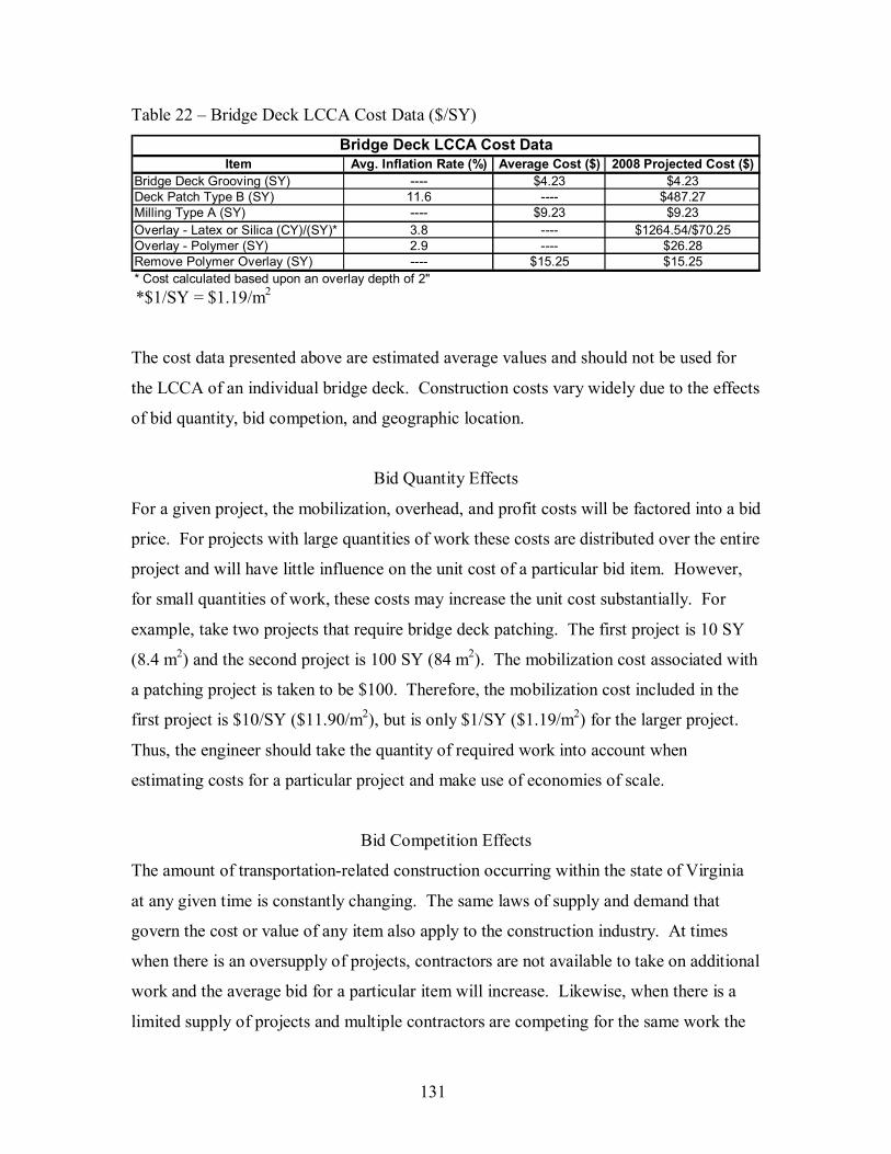
131

Table 22 � Bridge Deck LCCA Cost Data ($/SY)

*$1/SY = $1.19/m2

The cost data presented above are estimated average values and should not be used for

the LCCA of an individual bridge deck. Construction costs vary widely due to the effects

of bid quantity, bid competion, and geographic location.

Bid Quantity Effects

For a given project, the mobilization, overhead, and profit costs will be factored into a bid

price. For projects with large quantities of work these costs are distributed over the entire

project and will have little influence on the unit cost of a particular bid item. However,

for small quantities of work, these costs may increase the unit cost substantially. For

example, take two projects that require bridge deck patching. The first project is 10 SY

(8.4 m2) and the second project is 100 SY (84 m2). The mobilization cost associated with

a patching project is taken to be $100. Therefore, the mobilization cost included in the

first project is $10/SY ($11.90/m2), but is only $1/SY ($1.19/m2) for the larger project.

Thus, the engineer should take the quantity of required work into account when

estimating costs for a particular project and make use of economies of scale.

Bid Competition Effects

The amount of transportation-related construction occurring within the state of Virginia

at any given time is constantly changing. The same laws of supply and demand that

govern the cost or value of any item also apply to the construction industry. At times

when there is an oversupply of projects, contractors are not available to take on additional

work and the average bid for a particular item will increase. Likewise, when there is a

limited supply of projects and multiple contractors are competing for the same work the

Item Avg. Inflation Rate (%) Average Cost ($) 2008 Projected Cost ($)Bridge Deck Grooving (SY) ---- $4.23 $4.23Deck Patch Type B (SY) 11.6 ---- $487.27Milling Type A (SY) ---- $9.23 $9.23Overlay - Latex or Silica (CY)/(SY)* 3.8 ---- $1264.54/$70.25Overlay - Polymer (SY) 2.9 ---- $26.28Remove Polymer Overlay (SY) ---- $15.25 $15.25* Cost calculated based upon an overlay depth of 2"

Bridge Deck LCCA Cost Data

132

cost will be driven down. The effects that bid competition will have on an individual

project are difficult to estimate, however, attempts by maintenance engineers to maintain

steady work orders may help to negate these effects.

Geographic Location Effects

The effect that the location of a project has on cost can be substantial. Within Virginia,

labor and material costs can vary significantly. For example, the hourly wage of a

construction crewman in Northern Virginia is expected to be greater than for a crewman

in Roanoke. The distance of the project from the necessary resources is also an important

factor as the transportation costs for materials is often higher than the cost of the

materials themselves. For most cases district engineers will be able to accurately

estimate costs for their specific locality, but special cases may arise where the location of

the project warrants additional consideration. An example of this would be a bridge that

is located a great distance from a ready-mix plant. In that case it may be necessary to use

precast bridge panels rather than a cast-in-place bridge deck. This would affect the initial

costs of the project as well as the maintenance costs over the lifetime of the structure.

Traffic Control Costs

The traffic control (TC) costs related to a bridge deck maintenance project will vary by

location, route type, ADT, and duration. Therefore, there is no single value that can be

used for all LCCA�s. In the following examples an average TC cost of $5.88/ft2

($52.92/SY or $62.97/m2) will be used for concrete overlays. This value was

recommended in a previous study relating to bridge maintenance in Virginia. (Pyc et al,

2000) To estimate the TC costs associated with a polymer overlay, the duration of the

projects was considered. It is estimated that the application of a polymer overlay will

take approximately 1/3 of the time that is required for a concrete overlay. Therefore, the

reduction in TC costs should correspond with the reduction in construction time. Thus,

TC costs for polymer overlays will be taken to be 1/3 of concrete overlays or $1.96/ft2

($17.64/SY or $20.99/m2).

133

User Costs

User costs will not be considered initially. The primary focus of this LCCA is to estimate

the direct Agency costs that will be incurred for the two sets of bridge decks. A more

robust LCCA modeling program will be presented that is capable of estimating user costs

based upon the parameters of a given project. A detailed analysis of an individual bridge

deck will be presented to illustrate the capabilities of the available software.

Step 4: Compute Life-Cycle Costs

To compute the LCC�s for this project a deterministic approach has been taken. A

database of the distribution of times for specific maintenance events is not available.

Therefore, a probabilistic approach is not possible.

As mentioned previously, the discount rate that is specified for use by government

agencies is 5.1% for long-term projects. Therefore, a discount rate of 5.1% has been used

in the following examples. However, it may be necessary to adjust the long-term

discount rate to reflect the impacts of inflation.

Inflation Rates

It is common practice to use the CPI to compute the inflation of the general economy.

However, the application of the inflation rate associated with the CPI to transportation

related construction activities might not be valid because of the differences in the

inflation of different products and services. To determine the appropriate rate of inflation

for transportation construction activities three cost indexes were investigated:

Engineering News Record (ENR) Construction Cost Index, FHWA Composite

Construction Cost Index, and FHWA Structures Construction Cost Index. After the

inflation rates are determined for the three construction-related indexes they will be

compared to the CPI to determine if any significant differences are evident.

ENR Construction Cost Index (CCI)

The ENR CCI was developed as a means of tracking price trends in the construction

industry. The index measures the cost to purchase a set package of goods and services

134

compared to the cost of the same package in the base year. The base year for the CCI is

1913 and the index is composed of the 20-city average of the following components:

(Grogan, 2006)

• 200 hours of common labor

• 25 cwt of standard structural steel shapes (fabricated)

• 1,128 tons of Portland cement

• 1,088 board-ft of 2x4 lumber

The index for the time period of 1918 � 2005 is presented in Figure 52.

Figure 52 � ENR Construction Cost Index

Using the index values the average annual inflation rate was calculated and is presented

in Figure 53.

ENR Construction Cost Index

0

1000

2000

3000

4000

5000

6000

7000

8000

1918 1928 1938 1948 1958 1968 1978 1988 1998

Year

Ann

ual A

vera

ge

135

Figure 53 � CCI Average Annual Inflation Rate

As shown the CCI inflation rate was very volatile in the early 1900�s ranging from �

20%/year to 26%/year; however, it has become more stable in recent years. Over

approximately the last 20 years the inflation rate has ranged between 2 and 6%.

FHWA Composite Construction Cost Index

The FHWA Composite CCI tracks the costs of transportation construction projects that

are constructed using Federal funds. The Composite index consists of three

subcategories: Excavation, Resurfacing, and Structures with weightings of 21%, 36%,

and 43%, respectively. A base year of 1987 is used and the following components make

up the index:

• 210,078,000 cubic yards of roadway excavation,

• 30,893,690 square yards of portland cement concrete surfacing with an average

thickness of 9 inches,

• 37,760,443 tons of bituminous concrete surfacing,

• 577,753,544 pounds of reinforcing steel for structures,

• 444,924,141 pounds of structural steel, and

• 3,498,333 cubic yards of structural concrete.

CCI Average Annual Inflation Rate

-25

-20

-15

-10

-5

0

5

10

15

20

25

30

1918 1928 1938 1948 1958 1968 1978 1988 1998

Year

Ave

rage

Ann

ual I

nfla

tion

Rat

e (%

)

136

Only construction projects that exceed $500,000 in total cost are considered when

determining price trends for the index components.

In addition to a national cost index FHWA computes cost indexes for individual states.

However, care should be taken when determining inflation rates from a state index due to

high volatility. FHWA provides the following warning regarding state CCI�s.

�In some instances, individual State indices may not be truly representative of long-term

price trends because of comparatively low volumes of work for the period reported, or

because of unusual projects awarded during the period. Also, differences in bid item

specifications among the States might account for some of the differences in unit prices

in the various States.� (FHWA, 2006)

Due to the unreliability of state indexes, only the national index will be used in

determining inflation rates. The FHWA National Composite CCI is presented in Figure

54 and the corresponding inflation rates are presented in Figure 55.

Figure 54 � FHWA Composite CCI

FHWA Composite CCI

0

20

40

60

80

100

120

140

160

180

200

1972 1977 1982 1987 1992 1997 2002

Year

Ann

ual A

vera

ge

137

Figure 55 � FHWA Composite CCI � Average Annual Inflation Rate

As shown the FHWA Composite CCI is significantly more volatile than the ENR CCI

with inflation rates over the last 20 years ranging from �3 to 19%. The reason for this

increased volatility is not clear. Some fluctuation in cost data may be attributable to

changes in funding levels for individual states.

FHWA Structures Construction Cost Index

The FHWA Stuctures CCI is calculated using the same methodology as the Composite

CCI. The only differences between the two indexes are the components. The Structures

CCI only includes items that pertain directly to the construction of highway structures

and therefore may be a better predictor of inflation rates associated with bridge

construction. The components included are:

• 577,753,544 pounds of reinforcing steel for structures,

• 444,924,141 pounds of structural steel, and

• 3,498,333 cubic yards of structural concrete.

The FHWA National Structures CCI is presented in Figure 56 and the corresponding

inflation rates are presented in Figure 57.

FHWA Composite CCI - Average Annual Inflation Rate

-10

-5

0

5

10

15

20

25

30

35

40

1972 1977 1982 1987 1992 1997 2002

Year

Ave

rage

Ann

ual I

nfla

tion

Rat

e (%

)

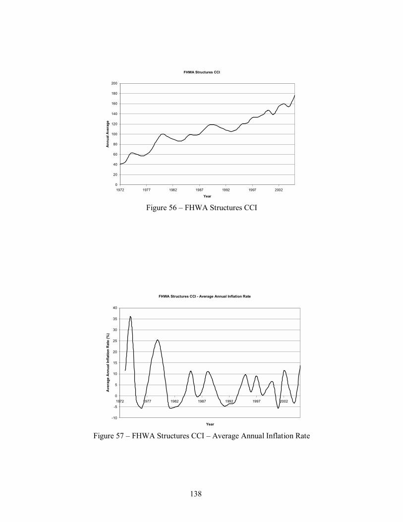
138

Figure 56 � FHWA Structures CCI

Figure 57 � FHWA Structures CCI � Average Annual Inflation Rate

FHWA Structures CCI

0

20

40

60

80

100

120

140

160

180

200

1972 1977 1982 1987 1992 1997 2002

Year

Ann

ual A

vera

ge

FHWA Structures CCI - Average Annual Inflation Rate

-10

-5

0

5

10

15

20

25

30

35

40

1972 1977 1982 1987 1992 1997 2002

Year

Ave

rage

Ann

ual I

nfla

tion

Rat

e (%

)

139

A comparison of the Structures CCI to the Composite CCI indicates that the two indexes

are very similar as might be expected.

Consumer Price Index (CPI)

The Consumer Price Index (CPI) is a �measure of the average change over time in the

prices paid by urban consumers for a market basket of consumer goods and services�.

(BLS, 2006) It is considered to be the most comprehensive measure of inflation for the

U.S. economy.

The CPI represents all goods and services purchased for consumption by a reference

population. The expenditure items included in the calculation of the CPI are arranged

into eight major groups. The groups are as follows:

• FOOD AND BEVERAGES (breakfast cereal, milk, coffee, chicken, wine, service

meals and snacks)

• HOUSING (rent of primary residence, owners' equivalent rent, fuel oil, bedroom

furniture)

• APPAREL (men's shirts and sweaters, women's dresses, jewelry)

• TRANSPORTATION (new vehicles, airline fares, gasoline, motor vehicle

insurance)

• MEDICAL CARE (prescription drugs and medical supplies, physicians' services,

eyeglasses and eye care, hospital services)

• RECREATION (televisions, pets and pet products, sports equipment, admissions);

• EDUCATION AND COMMUNICATION (college tuition, postage, telephone

services, computer software and accessories);

• OTHER GOODS AND SERVICES (tobacco and smoking products, haircuts and

other personal services, funeral expenses). (BLS, 2006)

The CPI is presented in Figure 58 and the corresponding inflation rates are presented in

Figure 59.

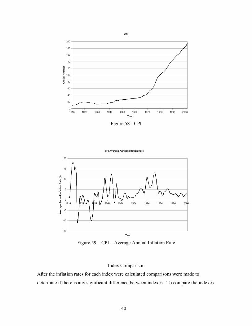
140

Figure 58 - CPI

Figure 59 � CPI � Average Annual Inflation Rate

Index Comparison

After the inflation rates for each index were calculated comparisons were made to

determine if there is any significant difference between indexes. To compare the indexes

CPI

0

20

40

60

80

100

120

140

160

180

200

1913 1923 1933 1943 1953 1963 1973 1983 1993 2003

Year

Ann

ual A

vera

ge

CPI Average Annual Inflation Rate

-15

-10

-5

0

5

10

15

20

1914 1924 1934 1944 1954 1964 1974 1984 1994 2004

Year

Ave

rage

Ann

ual I

nfla

tion

Rat

e (%

)

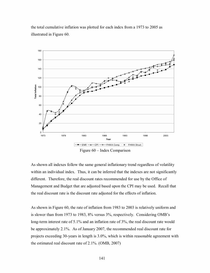
141

the total cumulative inflation was plotted for each index from a 1973 to 2005 as

illustrated in Figure 60.

Figure 60 � Index Comparison

As shown all indexes follow the same general inflationary trend regardless of volatility

within an individual index. Thus, it can be inferred that the indexes are not significantly

different. Therefore, the real discount rates recommended for use by the Office of

Management and Budget that are adjusted based upon the CPI may be used. Recall that

the real discount rate is the discount rate adjusted for the effects of inflation.

As shown in Figure 60, the rate of inflation from 1983 to 2003 is relatively uniform and

is slower than from 1973 to 1983, 8% versus 3%, respectively. Considering OMB�s

long-term interest rate of 5.1% and an inflation rate of 3%, the real discount rate would

be approximately 2.1%. As of January 2007, the recommended real discount rate for

projects exceeding 30-years in length is 3.0%, which is within reasonable agreement with

the estimated real discount rate of 2.1%. (OMB, 2007)

0

20

40

60

80

100

120

140

160

180

1973 1978 1983 1988 1993 1998 2003Year

Tota

l Inf

latio

n

ENR CPI FHWA Comp. FHWA Struct.

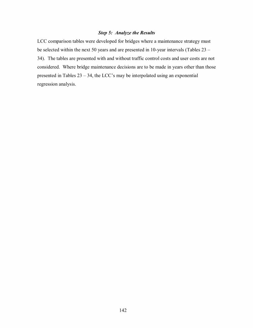
142

Step 5: Analyze the Results

LCC comparison tables were developed for bridges where a maintenance strategy must

be selected within the next 50 years and are presented in 10-year intervals (Tables 23 �

34). The tables are presented with and without traffic control costs and user costs are not

considered. Where bridge maintenance decisions are to be made in years other than those

presented in Tables 23 � 34, the LCC�s may be interpolated using an exponential

regression analysis.

143

Tab

le 2

3 �

LCC

Com

paris

on �

200

8 �

With

out T

raffi

c C

ontro

l

Tabl

e 24

� L

CC

Com

paris

on �

200

8 �

With

Tra

ffic

Con

trol

*$1/

SY =

$1.

19/m

2

2008

With

out T

raffi

c C

ontro

lY

ear

Ver

y H

igh

Hig

hM

oder

ate

0$3

0.19

$30.

19$3

0.19

$0.0

05

$20.

2510

$33.

81$1

7.46

15$2

9.17

$53.

7320

$25.

1625

$21.

7030

$18.

72$1

8.72

$9.6

735

$8.3

440

$13.

93$2

5.66

45$1

2.02

50$1

0.37

$10.

3755

$4.6

260

$7.7

1$7

.71

$3.9

865

$12.

2670

$5.7

475

$4.9

5$4

.95

80$4

.27

$2.2

185

$1.9

090

$3.1

8$3

.18

$5.8

595 10

0

* Rea

l Dis

coun

t Rat

e3.

00%

* AD

T: M

oder

ate

= 5,

000

to 2

5,00

0; H

igh

= >

25,0

00; V

ery

Hig

h =

> 50

,000

(Wey

ers

et a

l., 1

993)

Poly

mer

Ove

rlay

($/S

Y)Av

erag

e D

aily

Tra

ffic

(AD

T)

Required Remaining Service Life

Con

cret

e O

verla

y ($

/SY)

2008

With

Tra

ffic

Con

trol

Yea

rV

ery

Hig

hH

igh

Mod

erat

e0

$47.

83$4

7.83

$47.

83$0

.00

5$2

0.25

10$4

6.94

$17.

4615

$40.

49$8

7.70

20$3

4.93

25$3

0.13

30$2

5.99

$25.

99$9

.67

35$8

.34

40$1

9.34

$41.

8845

$16.

6850

$14.

39$1

4.39

55$4

.62

60$1

0.71

$10.

71$3

.98

65$2

0.00

70$7

.97

75$6

.87

$6.8

780

$5.9

3$2

.21

85$1

.90

90$4

.41

$4.4

1$9

.55

95 100

* AD

T: M

oder

ate

= 5,

000

to 2

5,00

0; H

igh

= >

25,0

00; V

ery

Hig

h =

> 50

,000

(Wey

ers

et a

l., 1

993)

Rea

l Dis

coun

t Rat

e3.

00%

Poly

mer

Ove

rlay

($/S

Y)Av

erag

e D

aily

Tra

ffic

(AD

T)C

oncr

ete

Ove

rlay

($/S

Y)


144

Tabl

e 25

� L

CC

Com

paris

on �

201

8 �

With

out T

raffi

c C

ontro

l

Tabl

e 26

� L

CC

Com

paris

on �

201

8 �

With

Tra

ffic

Con

trol

*$1/

SY =

$1.

19/m

2

2018

With

out T

raffi

c C

ontro

lY

ear

Ver

y H

igh

Hig

hM

oder

ate

0$2

2.46

$22.

46$2

2.46

$0.0

05

$15.

0610

$25.

16$1

2.99

15$2

1.70

$39.

9820

$18.

7225

$16.

1530

$13.

93$1

3.93

$7.1

935

$6.2

140

$10.

37$1

9.09

45$8

.94

50$7

.71

$7.7

155

$3.4

460

$5.7

4$5

.74

$2.9

665

$9.1

270

$4.2

775

$3.6

8$3

.68

80$3

.18

$1.6

485

$1.4

290

$2.3

6$2

.36

$4.3

695 10

0* A

DT:

Mod

erat

e =

5,00

0 to

25,

000;

Hig

h =

> 25

,000

; Ver

y H

igh

= >

50,0

00 (W

eyer

s et

al.,

199

3)R

eal D

isco

unt R

ate

3.00

%

Poly

mer

Ove

rlay

($/S

Y)Av

erag

e D

aily

Tra

ffic

(AD

T)


Con

cret

e O

verla

y ($

/SY)

2018

With

Tra

ffic

Con

trol

Yea

rV

ery

Hig

hH

igh

Mod

erat

e0

$35.

59$3

5.59

$35.

59$0

.00

5$1

5.06

10$3

4.93

$12.

9915

$30.

13$6

5.26

20$2

5.99

25$2

2.42

30$1

9.34

$19.

34$7

.19

35$6

.21

40$1

4.39

$31.

1745

$12.

4150

$10.

71$1

0.71

55$3

.44

60$7

.97

$7.9

7$2

.96

65$1

4.89

70$5

.93

75$5

.11

$5.1

180

$4.4

1$1

.64

85$1

.42

90$3

.28

$3.2

8$7

.11

95 100

* AD

T: M

oder

ate

= 5,

000

to 2

5,00

0; H

igh

= >

25,0

00; V

ery

Hig

h =

> 50

,000

(Wey

ers

et a

l., 1

993)

Rea

l Dis

coun

t Rat

e3.

00%


Con

cret

e O

verla

y ($

/SY)

Poly

mer

Ove

rlay

($/S

Y)Av

erag

e D

aily

Tra

ffic

(AD

T)

145

Tabl

e 27

� L

CC

Com

paris

on �

202

8 �

With

out T

raffi

c C

ontro

l

Tabl

e 28

� LC

C C

ompa

rison

� 2

028

� W

ith T

raff

ic C

ontro

l

*$1/

SY =

$1.

19/m

2

2028

With

out T

raffi

c C

ontro

lYe

arVe

ry H

igh

Hig

hM

oder

ate

0$1

6.72

$16.

72$1

6.72

$0.0

05

$11.

2110

$18.

72$9

.67

15$1

6.15

$29.

7520

$13.

9325

$12.

0230

$10.

37$1

0.37

$5.3

535

$4.6

240

$7.7

1$1

4.21

45$6

.65

50$5

.74

$5.7

455

$2.5

660

$4.2

7$4

.27

$2.2

165

$6.7

970

$3.1

875

$2.7

4$2

.74

80$2

.36

$1.2

285

$1.0

590

$1.7

6$1

.76

$3.2

495 10

0* A

DT:

Mod

erat

e =

5,00

0 to

25,

000;

Hig

h =

> 25

,000

; Ver

y H

igh

= >

50,0

00 (W

eyer

s et

al.,

199

3)* R

eal D

isco

unt R

ate

3.00

%

Poly

mer

Ove

rlay

($/S

Y)C

oncr

ete

Ove

rlay

($/S

Y)Av

erag

e D

aily

Tra

ffic

(AD

T)


2028

With

Tra

ffic

Con

trol

Year

Very

Hig

hH

igh

Mod

erat

e0

$26.

48$2

6.48

$26.

48$0

.00

5$1

1.21

10$2

5.99

$9.6

715

$22.

42$4

8.56

20$1

9.34

25$1

6.68

30$1

4.39

$14.

39$5

.35

35$4

.62

40$1

0.71

$23.

1945

$9.2

450

$7.9

7$7

.97

55$2

.56

60$5

.93

$5.9

3$2

.21

65$1

1.08

70$4

.41

75$3

.81

$3.8

180

$3.2

8$1

.22

85$1

.05

90$2

.44

$2.4

4$5

.29

95 100

* AD

T: M

oder

ate

= 5,

000

to 2

5,00

0; H

igh

= >

25,0

00; V

ery

Hig

h =

> 50

,000

(Wey

ers

et a

l., 1

993)

Rea

l Dis

coun

t Rat

e3.

00%

Poly

mer

Ove

rlay

($/S

Y)C

oncr

ete

Ove

rlay

($/S

Y)Av

erag

e D

aily

Tra

ffic

(AD

T)


146

Tabl

e 29

� L

CC

Com

paris

on �

203

8 �

With

out T

raffi

c C

ontro

l

Tabl

e 30

� L

CC

Com

paris

on �

203

8 �

With

Tra

ffic

Con

trol

*$1/

SY =

$1.

19/m

2

2038

With

out T

raffi

c C

ontro

lYe

arVe

ry H

igh

Hig

hM

oder

ate

0$1

2.44

$12.

44$1

2.44

$0.0

05

$8.3

410

$13.

93$7

.19

15$1

2.02

$22.

1420

$10.

3725

$8.9

430

$7.7

1$7

.71

$3.9

835

$3.4

440

$5.7

4$1

0.57

45$4

.95

50$4

.27

$4.2

755

$1.9

060

$3.1

8$3

.18

$1.6

465

$5.0

570

$2.3

675

$2.0

4$2

.04

80$1

.76

$0.9

185

$0.7

890

$1.3

1$1

.31

$2.4

195 10

0* A

DT:

Mod

erat

e =

5,00

0 to

25,

000;

Hig

h =

> 25

,000

; Ver

y H

igh

= >

50,0

00 (W

eyer

s et

al.,

199

3)R

eal D

isco

unt R

ate

3.00

%

Poly

mer

Ove

rlay

($/S

Y)C

oncr

ete

Ove

rlay

($/S

Y)Av

erag

e D

aily

Tra

ffic

(AD

T)


2038

With

Tra

ffic

Con

trol

Year

Very

Hig

hH

igh

Mod

erat

e0

$19.

71$1

9.71

$19.

71$0

.00

5$8

.34

10$1

9.34

$7.1

915

$16.

68$3

6.13

20$1

4.39

25$1

2.41

30$1

0.71

$10.

71$3

.98

35$3

.44

40$7

.97

$17.

2645

$6.8

750

$5.9

3$5

.93

55$1

.90

60$4

.41

$4.4

1$1

.64

65$8

.24

70$3

.28

75$2

.83

$2.8

380

$2.4

4$0

.91

85$0

.78

90$1

.82

$1.8

2$3

.94

95 100

* AD

T: M

oder

ate

= 5,

000

to 2

5,00

0; H

igh

= >

25,0

00; V

ery

Hig

h =

> 50

,000

(Wey

ers

et a

l., 1

993)

Rea

l Dis

coun

t Rat

e3.

00%

Poly

mer

Ove

rlay

($/S

Y)C

oncr

ete

Ove

rlay

($/S

Y)Av

erag

e D

aily

Tra

ffic

(AD

T)


147

Tabl

e 31

� L

CC

Com

paris

on �

204

8 �

With

out T

raffi

c C

ontro

l

Tabl

e 32

� L

CC

Com

paris

on �

204

8 �

With

Tra

ffic

Con

trol

*$1/

SY =

$1.

19/m

2

2048

With

out T

raffi

c C

ontro

lYe

arVe

ry H

igh

Hig

hM

oder

ate

0$9

.25

$9.2

5$9

.25

$0.0

05

$6.2

110

$10.

37$5

.35

15$8

.94

$16.

4720

$7.7

125

$6.6

530

$5.7

4$5

.74

$2.9

635

$2.5

640

$4.2

7$7

.87

45$3

.68

50$3

.18

$3.1

855

$1.4

260

$2.3

6$2

.36

$1.2

265

$3.7

670

$1.7

675

$1.5

2$1

.52

80$1

.31

$0.6

885

$0.5

890

$0.9

7$0

.97

$1.7

995 10

0* A

DT:

Mod

erat

e =

5,00

0 to

25,

000;

Hig

h =

> 25

,000

; Ver

y H

igh

= >

50,0

00 (W

eyer

s et

al.,

199

3)* R

eal D

isco

unt R

ate

3.00

%

Poly

mer

Ove

rlay

($/S

Y)C

oncr

ete

Ove

rlay

($/S

Y)A

vera

ge D

aily

Tra

ffic

(AD

T)


2048

With

Tra

ffic

Con

trol

Year

Very

Hig

hH

igh

Mod

erat

e0

$14.

66$1

4.66

$14.

66$0

.00

5$6

.21

10$1

4.39

$5.3

515

$12.

41$2

6.88

20$1

0.71

25$9

.24

30$7

.97

$7.9

7$2

.96

35$2

.56

40$5

.93

$12.

8445

$5.1

150

$4.4

1$4

.41

55$1

.42

60$3

.28

$3.2

8$1

.22

65$6

.13

70$2

.44

75$2

.11

$2.1

180

$1.8

2$0

.68

85$0

.58

90$1

.35

$1.3

5$2

.93

95 100

* AD

T: M

oder

ate

= 5,

000

to 2

5,00

0; H

igh

= >

25,0

00; V

ery

Hig

h =

> 50

,000

(Wey

ers

et a

l., 1

993)

Rea

l Dis

coun

t Rat

e3.

00%

Poly

mer

Ove

rlay

($/S

Y)C

oncr

ete

Ove

rlay

($/S

Y)A

vera

ge D

aily

Tra

ffic

(AD

T)


148

Tabl

e 33

� L

CC

Com

paris

on �

205

8 �

With

out T

raffi

c C

ontro

l

Tabl

e 34

� L

CC

Com

paris

on �

205

8 �

With

Tra

ffic

Con

trol

*$1/

SY =

$1.

19/m

2

2058

With

out T

raffi

c C

ontro

lYe

arVe

ry H

igh

Hig

hM

oder

ate

0$6

.89

$6.8

9$6

.89

$0.0

05

$4.6

210

$7.7

1$3

.98

15$6

.65

$12.

2620

$5.7

425

$4.9

530

$4.2

7$4

.27

$2.2

135

$1.9

040

$3.1

8$5

.85

45$2

.74

50$2

.36

$2.3

655

$1.0

560

$1.7

6$1

.76

$0.9

165

$2.8

070

$1.3

175

$1.1

3$1

.13

80$0

.97

$0.5

085

$0.4

390

$0.7

2$0

.72

$1.3

495 10

0* A

DT:

Mod

erat

e =

5,00

0 to

25,

000;

Hig

h =

> 25

,000

; Ver

y H

igh

= >

50,0

00 (W

eyer

s et

al.,

199

3)R

eal D

isco

unt R

ate

3.00

%

Poly

mer

Ove

rlay

($/S

Y)C

oncr

ete

Ove

rlay

($/S

Y)A

vera

ge D

aily

Tra

ffic

(AD

T)


2058

With

Tra

ffic

Con

trol

Year

Very

Hig

hH

igh

Mod

erat

e0

$10.

91$1

0.91

$10.

91$0

.00

5$4

.62

10$1

0.71

$3.9

815

$9.2

4$2

0.00

20$7

.97

25$6

.87

30$5

.93

$5.9

3$2

.21

35$1

.90

40$4

.41

$9.5

545

$3.8

150

$3.2

8$3

.28

55$1

.05

60$2

.44

$2.4

4$0

.91

65$4

.56

70$1

.82

75$1

.57

$1.5

780

$1.3

5$0

.50

85$0

.43

90$1

.01

$1.0

1$2

.18

95 100

* AD

T: M

oder

ate

= 5,

000

to 2

5,00

0; H

igh

= >

25,0

00; V

ery

Hig

h =

> 50

,000

(Wey

ers

et a

l., 1

993)

Rea

l Dis

coun

t Rat

e3.

00%

Poly

mer

Ove

rlay

($/S

Y)C

oncr

ete

Ove

rlay

($/S

Y)A

vera

ge D

aily

Tra

ffic

(AD

T)


149

Life Cycle Cost Comparison Examples

Several examples are presented below to illustrate the use of the LCC comparison tables.

Example 1:

Given: A maintenance strategy for a 30-year old bridge deck is to be selected in the

current year (2008). 0.5% of the bridge deck is presently deteriorated in the worst span

lane and the total desired service life of the bridge deck is 100 years. The ADT for the

bridge is 30,000 and traffic control is to be considered.

Solution: An ADT of 30,000 is considered high when determining the maintenance

schedule for the polymer overlays. Given that the bridge deck is 30 years old and the

desired service life is 100 years, the required remaining service life is 70 years. Using

Table 24 the LCCs are summed from year 0 � 70 for the two maintenance alternatives

being investigated (values to be summed are highlighted in Table 35).

Table 35 � LCCA � Example 1

*$1/SY = $1.19/m2

2008With Traffic Control

Year Very High High Moderate0 $47.83 $47.83 $47.83 $0.005 $20.25

10 $46.94 $17.4615 $40.49 $87.7020 $34.9325 $30.1330 $25.99 $25.99 $9.6735 $8.3440 $19.34 $41.8845 $16.6850 $14.39 $14.3955 $4.6260 $10.71 $10.71 $3.9865 $20.0070 $7.97

Sum $141.69 $213.9175 $6.87 $6.8780 $5.93 $2.2185 $1.9090 $4.41 $4.41 $9.5595100Sum $218.42 $294.67 $99.22 $441.48

* ADT: Moderate = 5,000 to 25,000; High = > 25,000; Very High = > 50,000 (Weyers et al., 1993)Real Discount Rate 3.00%

Polymer Overlay ($/SY)Average Daily Traffic (ADT)

Concrete Overlay ($/SY)

Req

uire

d R

emai

ning

Ser

vice

Life

150

Summing the LCCs for the two maintenance alternatives over the 70-year period yields

total LCCs of $141.70/SY ($168.62/m2) and $213.90/SY ($254.54/m2) for polymer

overlays and concrete overlays, respectively. Therefore, the decision in this case would

be to use polymer overlays to extend the service life of the bridge deck.

Example 2:

Given: The same bridge deck presented in Example 1 is to be considered. However,

now the ADT is 60,000 and the required remaining service life is only 25 years.

Solution: The LCCs to be summed are highlighted in Table 36.


*$1/SY = $1.19/m2

Summing the LCCs for the two maintenance alternatives over the 25-year period yields

total LCCs of $129.70/SY ($154.34/m2) and $125.41/SY ($149.24/m2) for polymer

overlays and concrete overlays, respectively. Therefore, the decision in this case would

be to use concrete overlays to extend the service life of the bridge deck. However, since


Year Very High High Moderate0 $47.83 $47.83 $47.83 $0.005 $20.2510 $46.94 $17.4615 $40.49 $87.7020 $34.9325 $30.13

Sum $129.69 $125.4130 $25.99 $25.99 $9.6735 $8.3440 $19.34 $41.8845 $16.6850 $14.39 $14.3955 $4.6260 $10.71 $10.71 $3.9865 $20.0070 $7.9775 $6.87 $6.8780 $5.93 $2.2185 $1.9090 $4.41 $4.41 $9.5595100Sum $348.11 $152.98 $99.22 $352.98

* ADT: Moderate = 5,000 to 25,000; High = > 25,000; Very High = > 50,000 (Weyers et al., 1993)Real Discount Rate 3.00%

Polymer Overlay ($/SY)Average Daily Traffic (ADT)

Concrete Overlay ($/SY)

Req

uire

d R

emai

ning

Ser

vice

Life

151

the difference between the two alternatives is small, the engineer may choose the higher

cost alternative based on other extenuating circumstances.

Example 3:

Given: A bridge deck is currently 20 years old and showing no signs of corrosion

deterioration. Using measured chloride concentrations, and cover depths, engineers have

estimated that the bridge deck will begin to reflect corrosion damage in approximately 20

years. The projected ADT of the bridge deck is 10,000 and the total desired service life

is 80 years. Traffic control will not be considered.

Solution: Given that the maintenance strategy is not to be selected in the current year,

but rather 20 years in the future, the Table for year 2028 will be used for the analysis.

The ADT is considered moderate and at the time of analysis the bridge deck will be 40

years old. Therefore, the required remaining service life will be 40 years.


*$1/SY = $1.19/m2

2028Without Traffic Control

Year Very High High Moderate0 $16.72 $16.72 $16.72 $0.005 $11.21

10 $18.72 $9.6715 $16.15 $29.7520 $13.9325 $12.0230 $10.37 $10.37 $5.3535 $4.6240 $7.71 $14.21

Sum $28.73 $74.8145 $6.6550 $5.74 $5.7455 $2.5660 $4.27 $4.27 $2.2165 $6.7970 $3.1875 $2.74 $2.7480 $2.36 $1.2285 $1.0590 $1.76 $1.76 $3.2495100

* ADT: Moderate = 5,000 to 25,000; High = > 25,000; Very High = > 50,000 (Weyers et al., 1993)* Real Discount Rate 3.00%

Polymer Overlay ($/SY) Concrete Overlay ($/SY)Average Daily Traffic (ADT)

Req

uire

d R

emai

ning

Ser

vice

Life

152

As shown in Table 37, the total LCCs for the maintenance alternatives are $28.74/SY

($34.20/m2) and $74.81/SY ($89.02/m2) for polymer overlays and concrete overlays,

respectively. Therefore, polymer overlays would be selected as the most cost effective

alternative.

Example 4:





Solution: A LCCA is not required for this example because polymer overlays are not

appropriate for bridge decks with total areas of corrsion deterioration greater than 1%.

Therefore, concrete overlays should be selected as the maintenance alternative for this

example.

Example 5:

Given: A bridge deck is reflecting between 0 and 1% corrosion deterioration in the worst

span lane and a maintenance strategy is to be selected in the current year. Due to

expected changes in traffic patterns the engineer is not able to accurately estimate future

traffic loads. The engineer is also unsure of what the required service life of the bridge

will be. Traffic control is to be considered.

Solution: Given the uncertainties in the problem the engineer can develop cash flow

charts using the tabulated LCC data to investigate the sensitivity of the analysis to

individual parameters. An example of a cash flow diagram for a bridge deck whose

maintenance strategy is to be selected in the current year is presented in Figure 61.

153

*$1/SY = $1.19/m2

Figure 61 � Cash Flow Diagram � Example 5

Using the cash flow diagram presented above, the engineer can investigate the effects of

varying traffic volumes on the selection of the appropriate maintenance strategy. As

shown, polymer overlays are the most economical option in nearly all cases. Concrete

overlays are more cost-effective only if the ADT is expected to be very high and the

required remaining service life falls within certain time frames. Therefore, due to the

uncertainty of the project the most economical alternative will most likely be polymer

overlays.

Maintenance Planning Costs

The maintenance alternative decisions presented in the previous section were based upon

total LCCs calculated using a discount rate of 3.0%. LCCAs are useful for determining

the most cost-effective maintenance alternative for a given bridge deck. However, it is

often the case that maintenance officials are interested in the total cost of a maintenance

0

50

100

150

200

250

0 10 20 30 40 50 60 70 80 90 100

Year

Cos

t ($/

SY)

Polymer Overlay - VH Polymer Overlay - H Polymer Overlay - M Concrete Overlay

154

alternative. Knowing the total cost of an alternative is useful in that there are inherent

risks when conducting LCCAs using estimated discount rates because if actual discount

rates differ from estimated rates the resulting LCCs may vary substantially. By

estimating the total inflated costs of maintenance alternatives the engineer can compare

alternatives based upon total expected costs. These comparisons will be void of any

benefit that is anticipated from saving money in the short-term. Additionally, by

computing actual costs the engineer can estimate the number of dollars that will be

required to maintain a bridge in any given year.

To estimate the total cost of a maintenance alternative, the project costs in future years

must be inflated from costs in the current year. Costs were increased using an inflation

rate of 3.0%, which was estimated for construction projects previously. The resulting

inflated costs for maintenance strategy decisions to be made within the next 50 years are

presented in Tables 38 � 49.

Future costs were calculated using the following time-value of money relationship:

niPVFV )1( +×= Equation 40

where:

FV = Future Value

PV = Present Value

i = Inflation rate

n = Number of years in the future

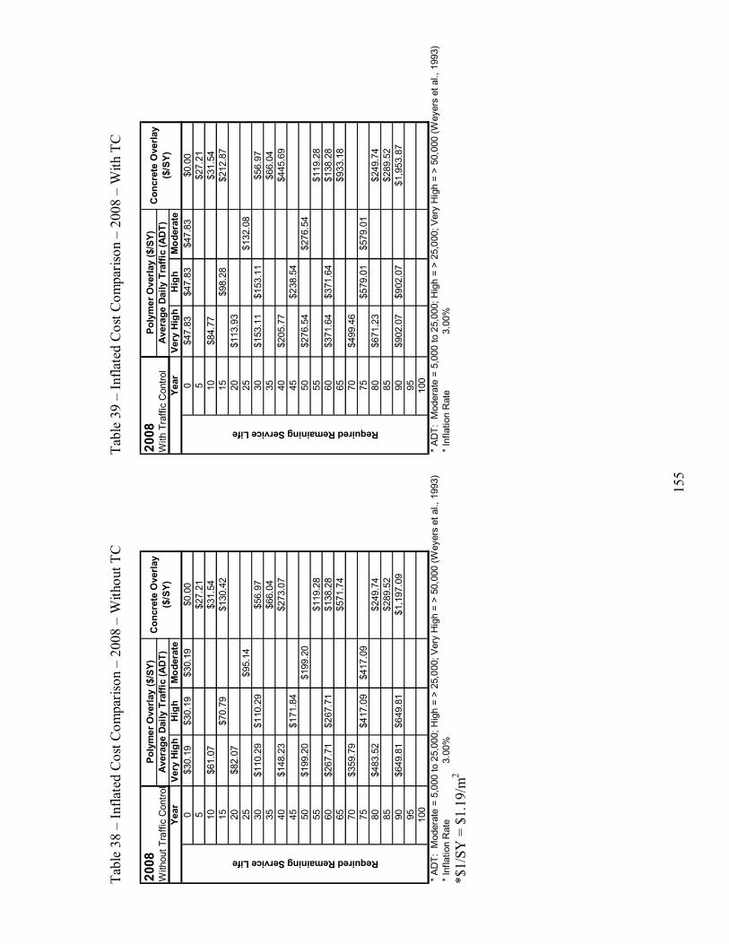
155

Tabl

e 38

� In

flate

d C

ost C

ompa

rison

� 2

008

� W

ithou

t TC

Tabl

e 39

� In

flate

d C

ost C

ompa

rison

� 2

008

� W

ith T

C

*$1/

SY =

$1.

19/m

2

2008

With

out T

raffi

c C

ontro

lYe

arVe

ry H

igh

Hig

hM

oder

ate

0$3

0.19

$30.

19$3

0.19

$0.0

05

$27.

2110

$61.

07$3

1.54

15$7

0.79

$130

.42

20$8

2.07

25$9

5.14

30$1

10.2

9$1

10.2

9$5

6.97

35$6

6.04

40$1

48.2

3$2

73.0

745

$171

.84

50$1

99.2

0$1

99.2

055

$119

.28

60$2

67.7

1$2

67.7

1$1

38.2

865

$571

.74

70$3

59.7

975

$417

.09

$417

.09

80$4

83.5

2$2

49.7

485

$289

.52

90$6

49.8

1$6

49.8

1$1

,197

.09

95 100

* Inf

latio

n R

ate

3.00

%

Poly

mer

Ove

rlay

($/S

Y)C

oncr

ete

Ove

rlay

($/S

Y)Av

erag

e Da

ily T

raffi

c (A

DT)


* AD

T: M

oder

ate

= 5,

000

to 2

5,00

0; H

igh

= >

25,0

00; V

ery

Hig

h =

> 50

,000

(Wey

ers

et a

l., 1

993)

2008

With

Tra

ffic

Con

trol

Year

Very

Hig

hH

igh

Mod

erat

e0

$47.

83$4

7.83

$47.

83$0

.00

5$2

7.21

10$8

4.77

$31.

5415

$98.

28$2

12.8

720

$113

.93

25$1

32.0

830

$153

.11

$153

.11

$56.

9735

$66.

0440

$205

.77

$445

.69

45$2

38.5

450

$276

.54

$276

.54

55$1

19.2

860

$371

.64

$371

.64

$138

.28

65$9

33.1

870

$499

.46

75$5

79.0

1$5

79.0

180

$671

.23

$249

.74

85$2

89.5

290

$902

.07

$902

.07

$1,9

53.8

795 10

0* A

DT:

Mod

erat

e =

5,00

0 to

25,

000;

Hig

h =

> 25

,000

; Ver

y H

igh

= >

50,0

00 (W

eyer

s et

al.,

199

3)* I

nfla

tion

Rat

e3.

00%

Poly

mer

Ove

rlay

($/S

Y)C

oncr

ete

Ove

rlay

($/S

Y)Av

erag

e Da

ily T

raffi

c (A

DT)


156

Tabl

e 40

� In

flate

d C

ost C

ompa

rison

� 2

018

� W

ithou

t TC

Tabl

e 41

� In

flate

d C

ost C

ompa

rison

� 2

018

� W

ith T

C

*$1/

SY =

$1.

19/m

2

2018

With

out T

raffi

c C

ontro

lYe

arVe

ry H

igh

Hig

hM

oder

ate

0$4

0.57

$40.

57$4

0.57

$0.0

05

$36.

5710

$82.

07$4

2.39

15$9

5.14

$175

.27

20$1

10.2

925

$127

.86

30$1

48.2

3$1

48.2

3$7

6.56

35$8

8.75

40$1

99.2

0$3

66.9

845

$230

.93

50$2

67.7

1$2

67.7

155

$160

.30

60$3

59.7

9$3

59.7

9$1

85.8

365

$768

.37

70$4

83.5

275

$560

.53

$560

.53

80$6

49.8

1$3

35.6

385

$389

.09

90$8

73.2

9$8

73.2

9$1

,608

.79

95 100

* AD

T: M

oder

ate

= 5,

000

to 2

5,00

0; H

igh

= >

25,0

00; V

ery

Hig

h =

> 50

,000

(Wey

ers

et a

l., 1

993)

* Inf

latio

n R

ate

3.00

%

Poly

mer

Ove

rlay

($/S

Y)C

oncr

ete

Ove

rlay

($/S

Y)Av

erag

e Da

ily T

raffi

c (A

DT)


2018

With

Tra

ffic

Con

trol

Year

Very

Hig

hH

igh

Mod

erat

e0

$64.

28$6

4.28

$64.

28$0

.00

5$3

6.57

10$1

13.9

3$4

2.39

15$1

32.0

8$2

86.0

720

$153

.11

25$1

77.5

030

$205

.77

$205

.77

$76.

5635

$88.

7540

$276

.54

$598

.97

45$3

20.5

850

$371

.64

$371

.64

55$1

60.3

060

$499

.46

$499

.46

$185

.83

65$1

,254

.12

70$6

71.2

375

$778

.14

$778

.14

80$9

02.0

7$3

35.6

385

$389

.09

90$1

,212

.31

$1,2

12.3

1$2

,625

.84

95 100

* AD

T: M

oder

ate

= 5,

000

to 2

5,00

0; H

igh

= >

25,0

00; V

ery

Hig

h =

> 50

,000

(Wey

ers

et a

l., 1

993)

* Inf

latio

n R

ate

3.00

%


Poly

mer

Ove

rlay

($/S

Y)C

oncr

ete

Ove

rlay

($/S

Y)Av

erag

e Da

ily T

raffi

c (A

DT)

157

Tabl

e 42

� In

flate

d C

ost C

ompa

rison

� 2

028

� W

ithou

t TC

Tabl

e 43

� In

flate

d C

ost C

ompa

rison

� 2

028

� W

ith T

C

*$1/

SY =

$1.

19/m

2

2028

With

out T

raffi

c C

ontro

lYe

arVe

ry H

igh

High

Mod

erat

e0

$54.

53$5

4.53

$54.

53$0

.00

5$4

9.14

10$1

10.2

9$5

6.97

15$1

27.8

6$2

35.5

520

$148

.23

25$1

71.8

430

$199

.20

$199

.20

$102

.89

35$1

19.2

840

$267

.71

$493

.19

45$3

10.3

550

$359

.79

$359

.79

55$2

15.4

360

$483

.52

$483

.52

$249

.74

65$1

,032

.62

70$6

49.8

175

$753

.31

$753

.31

80$8

73.2

9$4

51.0

685

$522

.90

90$1

,173

.63

$1,1

73.6

3$2

,162

.08

95 100

* AD

T: M

oder

ate

= 5,

000

to 2

5,00

0; H

igh

= >

25,0

00; V

ery

Hig

h =

> 50

,000

(Wey

ers

et a

l., 1

993)

* Inf

latio

n R

ate

3.00

%

Poly

mer

Ove

rlay

($/S

Y)C

oncr

ete

Ove

rlay

($/S

Y)Av

erag

e Da

ily T

raffi

c (A

DT)


2028

With

Tra

ffic

Con

trol

Year

Very

Hig

hHi

ghM

oder

ate

0$8

6.39

$86.

39$8

6.39

$0.0

05

$49.

1410

$153

.11

$56.

9715

$177

.50

$384

.46

20$2

05.7

725

$238

.54

30$2

76.5

4$2

76.5

4$1

02.8

935

$119

.28

40$3

71.6

4$8

04.9

745

$430

.84

50$4

99.4

6$4

99.4

655

$215

.43

60$6

71.2

3$6

71.2

3$2

49.7

465

$1,6

85.4

370

$902

.07

75$1

,045

.75

$1,0

45.7

580

$1,2

12.3

1$4

51.0

685

$522

.90

90$1

,629

.25

$1,6

29.2

5$3

,528

.91

95 100

* AD

T: M

oder

ate

= 5,

000

to 2

5,00

0; H

igh

= >

25,0

00; V

ery

Hig

h =

> 50

,000

(Wey

ers

et a

l., 1

993)

* Inf

latio

n R

ate

3.00

%

Poly

mer

Ove

rlay

($/S

Y)C

oncr

ete

Ove

rlay

($/S

Y)Av

erag

e Da

ily T

raffi

c (A

DT)


158

Tabl

e 44

� In

flate

d C

ost C

ompa

rison

� 2

038

� W

ithou

t TC

Tabl

e 45

� In

flate

d C

ost C

ompa

rison

� 2

038

� W

ith T

C

*$1/

SY =

$1.

19/m

2

2038

With

out T

raffi

c C

ontro

lYe

arVe

ry H

igh

High

Mod

erat

e0

$73.

28$7

3.28

$73.

28$0

.00

5$6

6.04

10$1

48.2

3$7

6.56

15$1

71.8

4$3

16.5

620

$199

.20

25$2

30.9

330

$267

.71

$267

.71

$138

.28

35$1

60.3

040

$359

.79

$662

.80

45$4

17.0

950

$483

.52

$483

.52

55$2

89.5

260

$649

.81

$649

.81

$335

.63

65$1

,387

.76

70$8

73.2

975

$1,0

12.3

9$1

,012

.39

80$1

,173

.63

$606

.19

85$7

02.7

490

$1,5

77.2

7$1

,577

.27

$2,9

05.6

695 10

0* A

DT:

Mod

erat

e =

5,00

0 to

25,

000;

Hig

h =

> 25

,000

; Ver

y H

igh

= >

50,0

00 (W

eyer

s et

al.,

199

3)* I

nfla

tion

Rat

e3.

00%

Poly

mer

Ove

rlay

($/S

Y)C

oncr

ete

Ove

rlay

($/S

Y)Av

erag

e Da

ily T

raffi

c (A

DT)


2038

With

Tra

ffic

Con

trol

Year

Very

Hig

hHi

ghM

oder

ate

0$1

16.1

0$1

16.1

0$1

16.1

0$0

.00

5$6

6.04

10$2

05.7

7$7

6.56

15$2

38.5

4$5

16.6

820

$276

.54

25$3

20.5

830

$371

.64

$371

.64

$138

.28

35$1

60.3

040

$499

.46

$1,0

81.8

145

$579

.01

50$6

71.2

3$6

71.2

355

$289

.52

60$9

02.0

7$9

02.0

7$3

35.6

365

$2,2

65.0

770

$1,2

12.3

175

$1,4

05.4

0$1

,405

.40

80$1

,629

.25

$606

.19

85$7

02.7

490

$2,1

89.5

7$2

,189

.57

$4,7

42.5

695 10

0* A

DT:

Mod

erat

e =

5,00

0 to

25,

000;

Hig

h =

> 25

,000

; Ver

y H

igh

= >

50,0

00 (W

eyer

s et

al.,

199

3)* I

nfla

tion

Rat

e3.

00%

Poly

mer

Ove

rlay

($/S

Y)C

oncr

ete

Ove

rlay

($/S

Y)Av

erag

e Da

ily T

raffi

c (A

DT)


159

Tabl

e 46

� In

flate

d C

ost C

ompa

rison

� 2

048

� W

ithou

t TC

Tabl

e 47

� In

flate

d C

ost C

ompa

rison

� 2

048

� W

ith T

C

*$1/

SY =

$1.

19/m

2

2048

With

out T

raffi

c C

ontro

lYe

arVe

ry H

igh

Hig

hM

oder

ate

0$9

8.48

$98.

48$9

8.48

$0.0

05

$88.

7510

$199

.20

$102

.89

15$2

30.9

3$4

25.4

320

$267

.71

25$3

10.3

530

$359

.79

$359

.79

$185

.83

35$2

15.4

340

$483

.52

$890

.75

45$5

60.5

350

$649

.81

$649

.81

55$3

89.0

960

$873

.29

$873

.29

$451

.06

65$1

,865

.03

70$1

,173

.63

75$1

,360

.56

$1,3

60.5

680

$1,5

77.2

7$8

14.6

785

$944

.42

90$2

,119

.72

$2,1

19.7

2$3

,904

.96

95 100

* AD

T: M

oder

ate

= 5,

000

to 2

5,00

0; H

igh

= >

25,0

00; V

ery

Hig

h =

> 50

,000

(Wey

ers

et a

l., 1

993)

* Inf

latio

n R

ate

3.00

%

Poly

mer

Ove

rlay

($/S

Y)C

oncr

ete

Ove

rlay

($/S

Y)Av

erag

e D

aily

Tra

ffic

(AD

T)


2048

With

Tra

ffic

Con

trol

Year

Very

Hig

hH

igh

Mod

erat

e0

$156

.02

$156

.02

$156

.02

$0.0

05

$88.

7510

$276

.54

$102

.89

15$3

20.5

8$6

94.3

720

$371

.64

25$4

30.8

430

$499

.46

$499

.46

$185

.83

35$2

15.4

340

$671

.23

$1,4

53.8

645

$778

.14

50$9

02.0

7$9

02.0

755

$389

.09

60$1

,212

.31

$1,2

12.3

1$4

51.0

665

$3,0

44.0

770

$1,6

29.2

575

$1,8

88.7

4$1

,888

.74

80$2

,189

.57

$814

.67

85$9

44.4

290

$2,9

42.6

0$2

,942

.60

$6,3

73.6

195 10

0* A

DT:

Mod

erat

e =

5,00

0 to

25,

000;

Hig

h =

> 25

,000

; Ver

y H

igh

= >

50,0

00 (W

eyer

s et

al.,

199

3)* I

nfla

tion

Rat

e3.

00%

Poly

mer

Ove

rlay

($/S

Y)C

oncr

ete

Ove

rlay

($/S

Y)Av

erag

e D

aily

Tra

ffic

(AD

T)


160

Tabl

e 48

� In

flate

d C

ost C

ompa

rison

� 2

058

� W

ithou

t TC

Tabl

e 49

� In

flate

d C

ost C

ompa

rison

� 2

058

� W

ith T

C

*$1/

SY =

$1.

19/m

2

2058

With

out T

raffi

c C

ontro

lYe

arVe

ry H

igh

Hig

hM

oder

ate

0$1

32.3

5$1

32.3

5$1

32.3

5$0

.00

5$1

19.2

810

$267

.71

$138

.28

15$3

10.3

5$5

71.7

420

$359

.79

25$4

17.0

930

$483

.52

$483

.52

$249

.74

35$2

89.5

240

$649

.81

$1,1

97.0

945

$753

.31

50$8

73.2

9$8

73.2

955

$522

.90

60$1

,173

.63

$1,1

73.6

3$6

06.1

965

$2,5

06.4

570

$1,5

77.2

775

$1,8

28.4

9$1

,828

.49

80$2

,119

.72

$1,0

94.8

485

$1,2

69.2

290

$2,8

48.7

2$2

,848

.72

$5,2

47.9

495 10

0* A

DT:

Mod

erat

e =

5,00

0 to

25,

000;

Hig

h =

> 25

,000

; Ver

y H

igh

= >

50,0

00 (W

eyer

s et

al.,

199

3)* I

nfla

tion

Rat

e3.

00%

Poly

mer

Ove

rlay

($/S

Y)C

oncr

ete

Ove

rlay

($/S

Y)Av

erag

e D

aily

Tra

ffic

(AD

T)


2058

With

Tra

ffic

Con

trol

Year

Very

Hig

hH

igh

Mod

erat

e0

$209

.68

$209

.68

$209

.68

$0.0

05

$119

.28

10$3

71.6

4$1

38.2

815

$430

.84

$933

.18

20$4

99.4

625

$579

.01

30$6

71.2

3$6

71.2

3$2

49.7

435

$289

.52

40$9

02.0

7$1

,953

.87

45$1

,045

.75

50$1

,212

.31

$1,2

12.3

155

$522

.90

60$1

,629

.25

$1,6

29.2

5$6

06.1

965

$4,0

90.9

870

$2,1

89.5

775

$2,5

38.3

1$2

,538

.31

80$2

,942

.60

$1,0

94.8

485

$1,2

69.2

290

$3,9

54.6

1$3

,954

.61

$8,5

65.5

995 10

0* A

DT:

Mod

erat

e =

5,00

0 to

25,

000;

Hig

h =

> 25

,000

; Ver

y H

igh

= >

50,0

00 (W

eyer

s et

al.,

199

3)* I

nfla

tion

Rat

e3.

00%

Poly

mer

Ove

rlay

($/S

Y)C

oncr

ete

Ove

rlay

($/S

Y)Av

erag

e D

aily

Tra

ffic

(AD

T)


161

The maintenance planning costs presented in Tables 38 � 49 were derived from the

maintenance activity timings presented in Table 50. These maintenance activities are the

same as those used in the previous LCCA examples.

Table 50 � Maintenance Activity Timings � Total Costs

Inflated Cost Comparison Examples

The examples presented in the LCCA section are revisited below to compare decisions

based upon LCCA methodology and total cost methodology.

Example 1:





Year VH H M0 PO & 1% P PO & 1% P PO & 1% P5 6% P10 OR, PO, & 1% P 6% P15 OR, PO, & 1% P M, CO, & G20 OR, PO, and 1%P25 OR, PO, & 1% P30 OR, PO, and 1%P OR, PO, & 1% P 6% P35 6% P40 OR, PO, and 1%P M, CO, & G45 OR, PO, & 1% P50 OR, PO, and 1%P OR, PO, & 1% P55 6% P60 OR, PO, and 1%P OR, PO, & 1% P 6% P65 M, CO, & G70 OR, PO, and 1%P75 OR, PO, & 1% P OR, PO, & 1% P80 OR, PO, and 1%P 6% P85 6% P90 OR, PO, and 1%P OR, PO, & 1% P M, CO, & G95

100* PO = Polymer Overlay; P = Patching; OR = Overlay Removal; M = Milling; CO = Concrete Overlay; G = Bridge Deck Grooving

Polymer OverlaysADT Concrete Overlays

162

Solution: An ADT of 30,000 is considered high when determining the maintenance

schedule for the polymer overlays. Given that the bridge deck is 30 years old and the

desired service life is 100 years, the required remaining service life is 70 years. Using

Table 39 the inflated costs are summed from year 0 � 70 for the two maintenance

alternatives being investigated (values to be summed are highlighted in Table 51).

Table 51 � Inflated Costs � Example 1

*$1/SY = $1.19/m2

Summing the inflated costs for the two maintenance alternatives over the 70-year period

yields total inflated costs of $909.40/SY ($1082.19/m2) and $2031.05/SY (2416.95/m2)

for polymer overlays and concrete overlays, respectively. Therefore, the decision in this

case would be to use polymer overlays to extend the service life of the bridge deck. As

shown, the maintenance alternative recommendation does not change when the total

inflated costs are considered in place of the total LCCs for this example.


Year Very High High Moderate0 $47.83 $47.83 $47.83 $0.005 $27.2110 $84.77 $31.5415 $98.28 $212.8720 $113.9325 $132.0830 $153.11 $153.11 $56.9735 $66.0440 $205.77 $445.6945 $238.5450 $276.54 $276.5455 $119.2860 $371.64 $371.64 $138.2865 $933.1870 $499.46

Sum $909.40 $2,031.0575 $579.01 $579.0180 $671.23 $249.7485 $289.5290 $902.07 $902.07 $1,953.8795

100Sum $3,326.35 $3,299.89 $1,035.45 $6,555.24

* ADT: Moderate = 5,000 to 25,000; High = > 25,000; Very High = > 50,000 (Weyers et al., 1993)* Inflation Rate 3.00%


Req

uire

d R

emai

ning

Ser

vice

Life

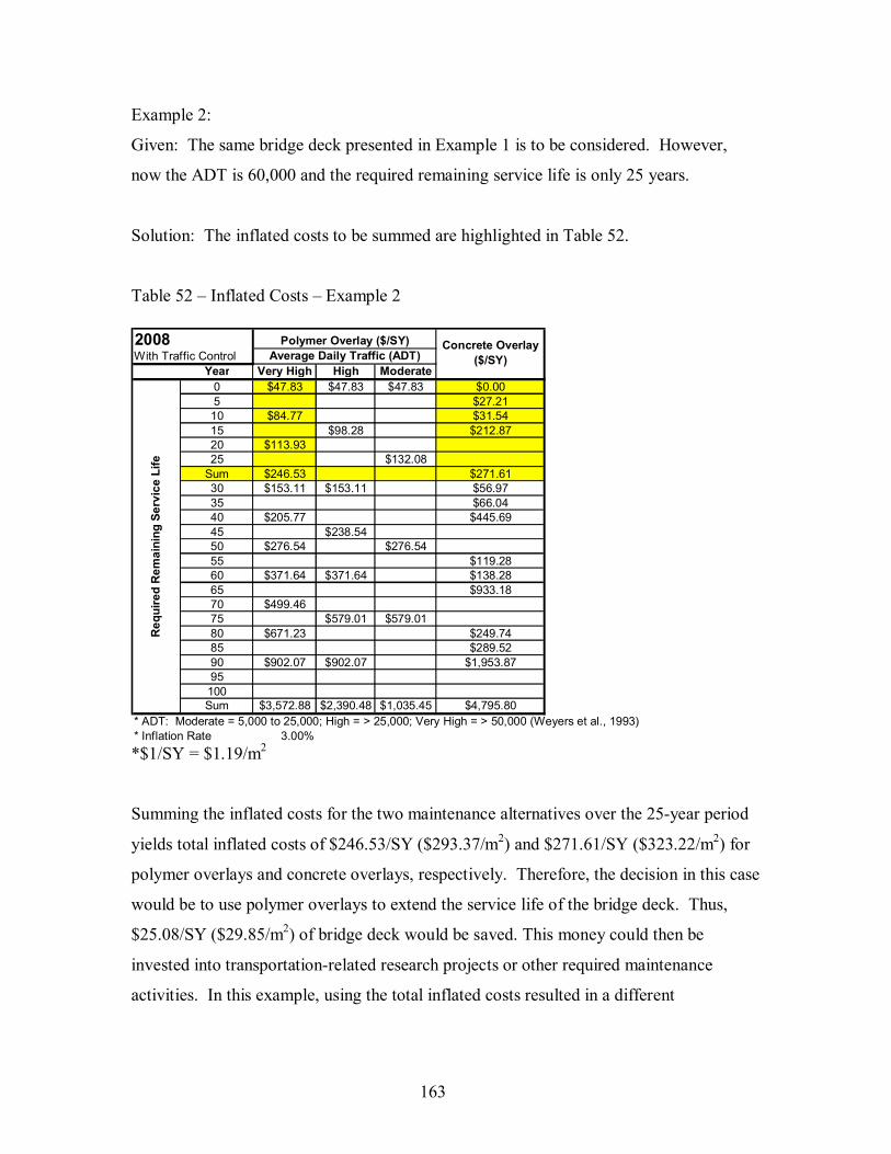
163

Example 2:

Given: The same bridge deck presented in Example 1 is to be considered. However,

now the ADT is 60,000 and the required remaining service life is only 25 years.

Solution: The inflated costs to be summed are highlighted in Table 52.


*$1/SY = $1.19/m2

Summing the inflated costs for the two maintenance alternatives over the 25-year period

yields total inflated costs of $246.53/SY ($293.37/m2) and $271.61/SY ($323.22/m2) for

polymer overlays and concrete overlays, respectively. Therefore, the decision in this case

would be to use polymer overlays to extend the service life of the bridge deck. Thus,

$25.08/SY ($29.85/m2) of bridge deck would be saved. This money could then be

invested into transportation-related research projects or other required maintenance

activities. In this example, using the total inflated costs resulted in a different


Year Very High High Moderate0 $47.83 $47.83 $47.83 $0.005 $27.2110 $84.77 $31.5415 $98.28 $212.8720 $113.9325 $132.08

Sum $246.53 $271.6130 $153.11 $153.11 $56.9735 $66.0440 $205.77 $445.6945 $238.5450 $276.54 $276.5455 $119.2860 $371.64 $371.64 $138.2865 $933.1870 $499.4675 $579.01 $579.0180 $671.23 $249.7485 $289.5290 $902.07 $902.07 $1,953.8795100Sum $3,572.88 $2,390.48 $1,035.45 $4,795.80



Req

uire

d R

emai

ning

Ser

vice

Life

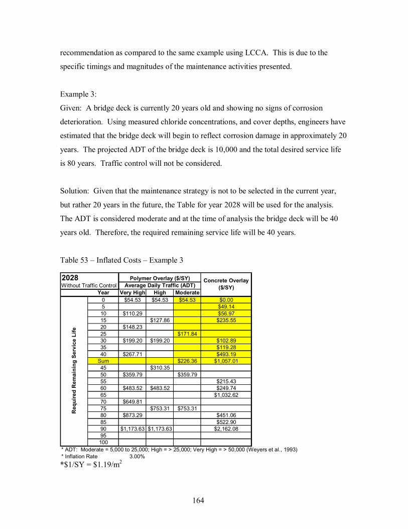
164

recommendation as compared to the same example using LCCA. This is due to the

specific timings and magnitudes of the maintenance activities presented.

Example 3:

Given: A bridge deck is currently 20 years old and showing no signs of corrosion

deterioration. Using measured chloride concentrations, and cover depths, engineers have

estimated that the bridge deck will begin to reflect corrosion damage in approximately 20

years. The projected ADT of the bridge deck is 10,000 and the total desired service life

is 80 years. Traffic control will not be considered.

Solution: Given that the maintenance strategy is not to be selected in the current year,

but rather 20 years in the future, the Table for year 2028 will be used for the analysis.

The ADT is considered moderate and at the time of analysis the bridge deck will be 40

years old. Therefore, the required remaining service life will be 40 years.


*$1/SY = $1.19/m2

2028Without Traffic Control

Year Very High High Moderate0 $54.53 $54.53 $54.53 $0.005 $49.1410 $110.29 $56.9715 $127.86 $235.5520 $148.2325 $171.8430 $199.20 $199.20 $102.8935 $119.2840 $267.71 $493.19

Sum $226.36 $1,057.0145 $310.3550 $359.79 $359.7955 $215.4360 $483.52 $483.52 $249.7465 $1,032.6270 $649.8175 $753.31 $753.3180 $873.29 $451.0685 $522.9090 $1,173.63 $1,173.63 $2,162.0895100



Req

uire

d R

emai

ning

Ser

vice

Life

165

As shown in Table 53, the total inflated costs for the maintenance alternatives are

$226.37/SY ($269.38/m2) and $1057.02/SY ($1257.85/m2) for polymer overlays and

concrete overlays, respectively. Therefore, polymer overlays would be selected as the

most cost effective alternative.

Example 4:





Solution: A total maintenance cost analysis is not required for this example because

polymer overlays are not appropriate for bridge decks with total areas of corrsion

deterioration greater than 1%. Therefore, concrete overlays should be selected as the

maintenance alternative for this example.

Example 5:

Given: A bridge deck is reflecting between 0 and 1% corrosion deterioration in the worst

span lane and a maintenance strategy is to be selected in the current year. Due to

expected changes in traffic patterns the engineer is not able to accurately estimate future

traffic loads. The engineer is also unsure of what the required service life of the bridge

will be. Traffic control is to be considered.

Solution: Given the uncertainties in the problem the engineer can develop cash flow

charts using the tabulated inflated cost data to investigate the sensitivity of the analysis to

individual parameters. An example of a cash flow diagram for a bridge deck whose

maintenance strategy is to be selected in the current year is presented in Figure 62.

166

*$1/SY = $1.19/m2

Figure 62 � Cash Flow Diagram � Inflated Costs � Example 5

Using the cash flow diagram presented above, the engineer can investigate the effects that

varying traffic volumes will have on the selection of the appropriate maintenance

strategy. As shown, polymer overlays are the most economical option in nearly all cases.

Concrete overlays are more cost-effective only if the ADT is expected to be very high

and the required remaining service life falls within certain time frames. Therefore, due to

the uncertainty of the project the most economical alternative will most likely be polymer

overlays. It is important to note that this total cost analysis results in the same

recommendations as the LCCA.

The total cost approach is not expected to affect the maintenance alternative selected in

most cases. However, it will provide useful data concerning the anticipated costs to be

incurred in the future. By knowing the timings and amounts of future maintenance

expenditures the engineer can better plan and budget maintenance activities.

0

500

1000

1500

2000

2500

3000

3500

4000

4500

5000

0 10 20 30 40 50 60 70 80 90 100

Year

Cos

t ($/

SY)

Polymer Overlay - VH Polymer Overlay - H Polymer Overlay - M Concrete Overlay

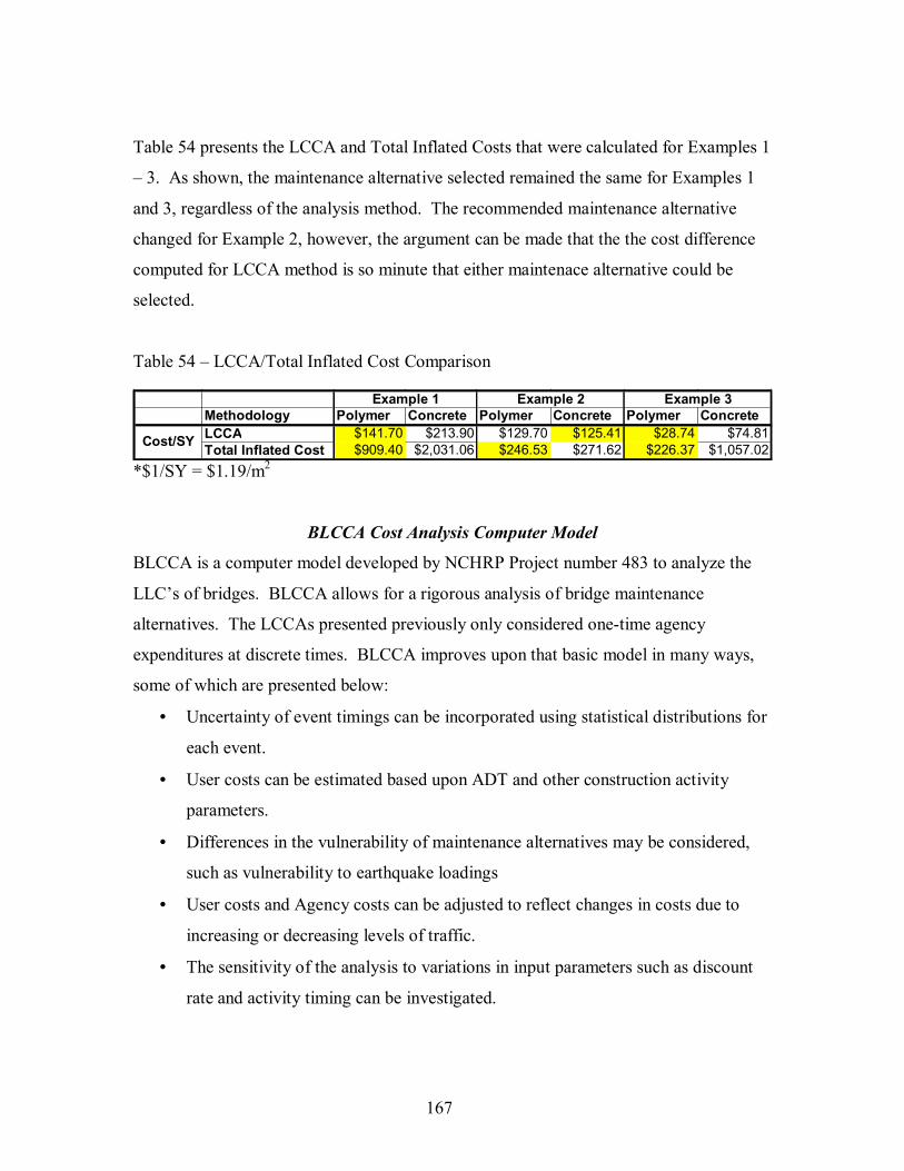
167

Table 54 presents the LCCA and Total Inflated Costs that were calculated for Examples 1

� 3. As shown, the maintenance alternative selected remained the same for Examples 1

and 3, regardless of the analysis method. The recommended maintenance alternative

changed for Example 2, however, the argument can be made that the the cost difference

computed for LCCA method is so minute that either maintenace alternative could be

selected.

Table 54 � LCCA/Total Inflated Cost Comparison

*$1/SY = $1.19/m2

BLCCA Cost Analysis Computer Model

BLCCA is a computer model developed by NCHRP Project number 483 to analyze the

LLC�s of bridges. BLCCA allows for a rigorous analysis of bridge maintenance

alternatives. The LCCAs presented previously only considered one-time agency

expenditures at discrete times. BLCCA improves upon that basic model in many ways,

some of which are presented below:

• Uncertainty of event timings can be incorporated using statistical distributions for

each event.

• User costs can be estimated based upon ADT and other construction activity

parameters.

• Differences in the vulnerability of maintenance alternatives may be considered,

such as vulnerability to earthquake loadings

• User costs and Agency costs can be adjusted to reflect changes in costs due to

increasing or decreasing levels of traffic.

• The sensitivity of the analysis to variations in input parameters such as discount

rate and activity timing can be investigated.

Methodology Polymer Concrete Polymer Concrete Polymer ConcreteLCCA $141.70 $213.90 $129.70 $125.41 $28.74 $74.81Total Inflated Cost $909.40 $2,031.06 $246.53 $271.62 $226.37 $1,057.02Cost/SY

Example 1 Example 2 Example 3

168

• Before, during, and after maintenance activity effects can be considered. For

example user costs associated with accidents may be reduced due to the widening

of a bridge.

BLCCA is capable of providing a much more detailed analysis than would typically be

required. Input to the computer model can be adjusted to provide the level of analysis

desired for any individual project. Many times the engineer will only be concerned about

the Agency costs associated with maintenance alternatives, in which case the use of a

robust computer model such as BLCCA may not be necessary. Additionally, care should

be taken when assigning values to input parameters as the effects on the analysis can be

substantial. To provide a complete analysis with BLCCA detailed input data concerning

anticipated ADT growth, vunerability costs, activity-timing distributions, and discount

rate variability is required.

An example of a LCCA using BLCCA is presented in the following section. The

example uses the same input data that was used in an example presented previously and

also incorporates estimated values for user costs, uniform maintenance costs, and ADT.

1.0 BLCCA Example

This is an example of a LCC comparison between two bridge maintenance alternatives.

The two maintenance alternatives are the same as those presented previously (Polymer

Overlays and Concrete Overlays). Values presented are intended to provide an

approximate representation of a typical bridge deck. This example is a modified version

of Example 1 presented in the BLCCA Users Manual. (BLCCA, 2003) The BLCCA

Users Manual is to be consulted for an in-depth description of the computer model.

1.1 Structure Description

The bridge to be analyzed has a total area of 2000 SF (222 SY) with a design life of 100

years.

169

1.2 BLCCA Data Input

1.2.1 Bridge

The first step in conducting a LCCA in BLCCA is to select a bridge and comparison type

from the provided bridge inventory. The BLCCA inventory includes a variety of

predefined life cycle comparison templates for alternatives such as overlay type and

structure widening. BLCCA also contains a database of NBI structure numbers that

allows for the user to select the specific bridge to be analyzed. If the bridge is included in

the NBI database, the parameters of the bridge such as the length and width will be

automatically defined. The bridge in this example is not in the NBI database, so the �Not

Defined� bridge must be selected, and appropriate data corrected/added throughout the

four Inventory tabs of BLCCA data input.

1.2.2 New Scenario Definition

New scenario definition involves the specification of the analysis period, discount rate

and the selection of primary model types to be used for all life-cycle analyses.

The length of analysis period is set to 100 years for this example. This selection was

made to reflect the requirement for both alternatives to last at least 100 years. It is also

assumed that at year 100 neither of the two alternatives will have any residual (salvage)

value, and that at this year the construction-repair cycle will restart.

Federal Infrastructure Projects use discount rates published in OMB Circular No. A-94.

Since the length of analysis will be 100 years, a Discount Rate of 3.00% will be used just

as in the examples presented previously.

The primary model types that may be considered in BLCCA are Traffic Projection,

Condition Index, and Load Capacity. By defining an ADT that increases with time the

associated increase in user costs will be included in the LCCA. Changes in the Condition

Index and Load Capacity primary models will not affect the LCC�s computed by

BLCCA, but can be used by the engineer to monitor the overall condition of the structure

over its service life. The primary models are by default set to �generic�; this selection

170

will accommodate the data input for this example.

1.2.3 Initial Condition Definition

The first primary model to be defined is the Average Daily Traffic (ADT). The example

conditions are such that at year 1 the ADT is equal to 20,000 vehicles, and that at year

100 the ADT is equal to 40,000 vehicles. A two-point curve definition is sufficient to

define the ADT projection line.

Table 55 � ADT Primary Model

The second primary model is the Condition Index. A Condition index of 100 reflects a

perfect condition (immediately after initial construction), while 50 would require

significant repair. In this example the bridge deck is expected to require significant

repair at 35 years of age. The intermediate condition index at year 20 was chosen to

reflect the case where the bridge condition deteriorates faster as time progresses.

Table 56 � Condition Index Primary Model

The third primary model is the Load Capacity. The Load Capacity is taken to be 36 tons

and remains constant. This indicates that corrosion of the bridge deck will not affect the

load capacity of the structure. The load capacity of the structure is also irrelevant for a

LCCA concerning bridge deck overlays.

Table 57 � Load Capacity Primary Model

Year Index0 10020 8535 50

Condition Index

Year Capacity (tons)0 36

100 36

Load Capacity

Year ADT0 20000

100 40000

Traffic Summary Table

171

1.2.4 Initial Cost Definition

This example does not consider any vulnerability costs. The only initial cost that the

bridge will experience is due to NBI Inspections (Distributed Agency Cost): $150 every

two years.

BLCCA requires input in equivalent annual cost. Therefore, the inspection costs are set

at a constant rate of $75 per year. Furthermore, it is expected that the inspections will not

begin until 2 years after the construction. To reflect this delay, a timeshift of 3 years will

be used.

Table 58 � Agency Maintenance Costs

1.3 Alternative 1 � Polymer Overlays

BLCCA does not require detailed item-by-item cost data input. It is only necessary to

provide the total costs associated with a particular event. For example, for an overlay it is

not necessary to provide indvidual costs for patching, traffic control, and overlay

materials if all of the costs occur in the same year. The user can simply provide an

estimated cost for the project as a whole.

The definition of alternatives can be performed using either the Wizard or the

Event/Effects tab. To illustrate both options, Alternative 1 will be defined using the

Wizard, and Alternative 2 using Event/Effects tab.

1.3.1 Wizard � Polymer Overlays

The Wizard guides the user through a series of steps to define the events and their effects.

Alternative 1, Polymer Overlays, involves 5 events and each event lasts 1 year (or less):

Year Cost0 75

100 75* Timeshift of 3 years

Distributed Agency Costs

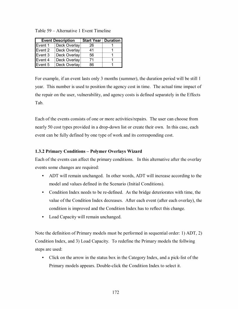
172

Table 59 � Alternative 1 Event Timeline

For example, if an event lasts only 3 months (summer), the duration period will be still 1

year. This number is used to position the agency cost in time. The actual time impact of

the repair on the user, vulnerability, and agency costs is defined separately in the Effects

Tab.

Each of the events consists of one or more activities/repairs. The user can choose from

nearly 50 cost types provided in a drop-down list or create their own. In this case, each

event can be fully defined by one type of work and its corresponding cost.

1.3.2 Primary Conditions � Polymer Overlays Wizard

Each of the events can affect the primary conditions. In this alternative after the overlay

events some changes are required:

• ADT will remain unchanged. In other words, ADT will increase according to the

model and values defined in the Scenario (Initial Conditions).

• Condition Index needs to be re-defined. As the bridge deteriorates with time, the

value of the Condition Index decreases. After each event (after each overlay), the

condition is improved and the Condition Index has to reflect this change.

• Load Capacity will remain unchanged.

Note the definition of Primary models must be performed in sequential order: 1) ADT, 2)

Condition Index, and 3) Load Capacity. To redefine the Primary models the follwing

steps are used:

• Click on the arrow in the status box in the Category Index, and a pick-list of the

Primary models appears. Double-click the Condition Index to select it.

Start Year DurationEvent 1 Deck Overlay 26 1Event 2 Deck Overlay 41 1Event 3 Deck Overlay 56 1Event 4 Deck Overlay 71 1Event 5 Deck Overlay 86 1

Event Description

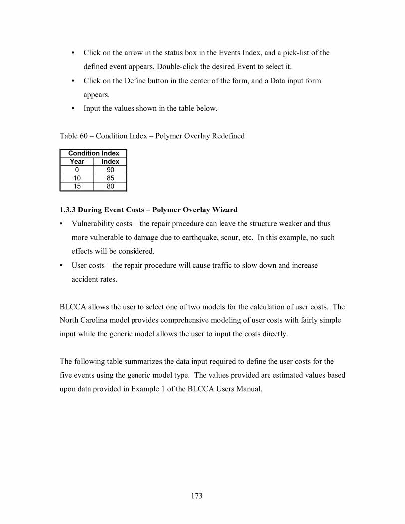
173

• Click on the arrow in the status box in the Events Index, and a pick-list of the

defined event appears. Double-click the desired Event to select it.

• Click on the Define button in the center of the form, and a Data input form

appears.

• Input the values shown in the table below.

Table 60 � Condition Index � Polymer Overlay Redefined

1.3.3 During Event Costs � Polymer Overlay Wizard

• Vulnerability costs � the repair procedure can leave the structure weaker and thus

more vulnerable to damage due to earthquake, scour, etc. In this example, no such

effects will be considered.

• User costs � the repair procedure will cause traffic to slow down and increase

accident rates.

BLCCA allows the user to select one of two models for the calculation of user costs. The

North Carolina model provides comprehensive modeling of user costs with fairly simple

input while the generic model allows the user to input the costs directly.

The following table summarizes the data input required to define the user costs for the

five events using the generic model type. The values provided are estimated values based

upon data provided in Example 1 of the BLCCA Users Manual.

Year Index0 9010 8515 80

Condition Index

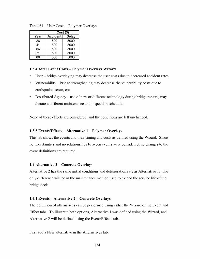
174

Table 61 � User Costs � Polymer Overlays

1.3.4 After Event Costs � Polymer Overlays Wizard

• User � bridge overlaying may decrease the user costs due to decreased accident rates.

• Vulnerability � bridge strengthening may decrease the vulnerability costs due to

earthquake, scour, etc.

• Distributed Agency � use of new or different technology during bridge repairs, may

dictate a different maintenance and inspection schedule.

None of these effects are considered, and the conditions are left unchanged.

1.3.5 Events/Effects � Alternative 1 � Polymer Overlays

This tab shows the events and their timing and costs as defined using the Wizard. Since

no uncertainties and no relationships between events were considered, no changes to the

event definitions are required.

1.4 Alternative 2 � Concrete Overlays

Alternative 2 has the same initial conditions and deterioration rate as Alternative 1. The

only difference will be in the maintenance method used to extend the service life of the

bridge deck.

1.4.1 Events � Alternative 2 � Concrete Overlays

The definition of alternatives can be performed using either the Wizard or the Event and

Effect tabs. To illustrate both options, Alternative 1 was defined using the Wizard, and

Alternative 2 will be defined using the Event/Effects tab.

First add a New alternative in the Alternatives tab.

Year Accident Delay26 500 500041 500 500056 500 500071 500 500086 500 5000

Cost ($)

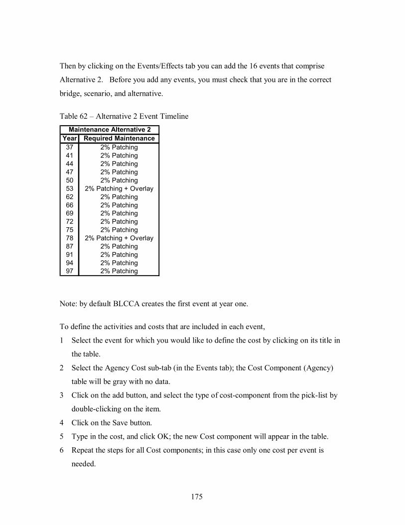
175

Then by clicking on the Events/Effects tab you can add the 16 events that comprise

Alternative 2. Before you add any events, you must check that you are in the correct

bridge, scenario, and alternative.

Table 62 � Alternative 2 Event Timeline

Note: by default BLCCA creates the first event at year one.

To define the activities and costs that are included in each event,

1 Select the event for which you would like to define the cost by clicking on its title in

the table.

2 Select the Agency Cost sub-tab (in the Events tab); the Cost Component (Agency)

table will be gray with no data.

3 Click on the add button, and select the type of cost-component from the pick-list by

double-clicking on the item.

4 Click on the Save button.

5 Type in the cost, and click OK; the new Cost component will appear in the table.

6 Repeat the steps for all Cost components; in this case only one cost per event is

needed.

Year Required Maintenance37 2% Patching41 2% Patching44 2% Patching47 2% Patching50 2% Patching53 2% Patching + Overlay62 2% Patching66 2% Patching69 2% Patching72 2% Patching75 2% Patching78 2% Patching + Overlay87 2% Patching91 2% Patching94 2% Patching97 2% Patching

Maintenance Alternative 2

176

7 Select the event Definition sub-tab, click on Event 2, and repeat the above-described

steps.

Please refer to the previous examples for the type of Cost components and associated

costs for Alternative 2.

1.4.2 Effects � Alternative 2 � Concrete Overlays

The effects for Alternative 2 on the primary conditions are the same as those for

Alternative 1 with the exception of the effect on the Condition Index. The Condition

Index after the event is adjusted as follows:

Table 63 � Condition Index � Concrete Overlay Redefined

The after event and during event costs are also the same as for Alternative 1 with the

exception of user costs. The user costs associated with Alternative 2 are higher due to

increased construction times. The appropriate values for Alternative 2 are presented

below.

Table 64 � User Costs � Concrete Overlays

1.5 Analysis Results

There are many reports and charts that can be generated by BLCCA to analyze the results

of the analysis, some of which are presented below.

Year Index0 9015 8025 40

Condition Index

Year Accident Delay53 1500 1500078 1500 15000

Cost ($)

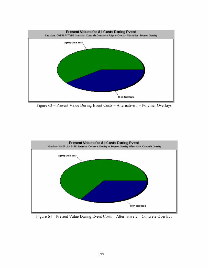
177

Figure 63 � Present Value During Event Costs � Alternative 1 � Polymer Overlays

Figure 64 � Present Value During Event Costs � Alternative 2 � Concrete Overlays

178

Figure 65 � Cumulative During Event Costs � Alternative 1 � Polymer Overlays

Figure 66 � Cumulative During Event Costs � Alternative 2 � Concrete Overlays

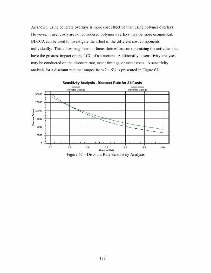
179

As shown, using concrete overlays is more cost effective than using polymer overlays.

However, if user costs are not considered polymer overlays may be more economical.

BLCCA can be used to investigate the affect of the different cost components

individually. This allows engineers to focus their efforts on optimizing the activities that

have the greatest impact on the LCC of a structure. Additionally, a sensitivity analyses

may be conducted on the discount rate, event timings, or event costs. A sensitivity

analysis for a discount rate that ranges from 2 � 5% is presented in Figure 67.

Figure 67 � Discount Rate Sensitivity Analysis

180

CONCLUSIONS

The following conclusions can be made from the results of this study:

1. The time to first repair and rehabilitation of bridge decks can be modeled using a

probabilistic approach, which allows for the incorporation of variability related to

chloride exposure conditions, bridge deck construction, and corrosion initiation.

2. Fick�s second law of diffusion can be used to model the apparent diffusion rate of

chlorides into a concrete bridge deck. Additionally, the effective diffusion rate at any

point in time can be projected using available diffusion decay models.

3. The time required for corrosion to induce cracking in the cover concrete can be

estimated using existing corrosion-cracking models. An estimated time to corrosion

cracking of 6 years for bare steel reinforcement was determined for this study using

the Liu/Weyers model in conjunction with the Vu, Stewart, and Mullard model.

4. The time to first repair for the set of 10 � 0.47 w/c bridge decks in Virginia can be

accurately predicted using the probabilistic service life model. However, accurate

service life predictions for individual bridge decks do not appear to be possible given

the limited amount of data available.

5. A reasonable estimate of the time required for corrosion deterioration to progress

from a level of 2% to a level of 12% was determined from damage surveys conducted

on actively corroding bridge decks. The corrosion propagation time for bare steel

bridge decks is estimated to be 16 years.

6. The reduction of the w/c ratio from 0.47 to 0.45 appears to have a negligible effect on

the diffusion properties of concrete.

7. The addition of pozzolan to the concrete mixture appears to dramatically reduce the

diffusion rate of chlorides into concrete.

181

8. The service lives of bridge decks constructed under current specifications (0.45 w/c+p

and 50 mm (in.) cover depth) are expected to exceed a design life of 100 years

regardless of reinforcement type.

9. Surface chloride concentrations, Co, have been determined for the Commonwealth of

Virginia and are only a function of the environmental exposure conditions not the

type of concrete.

10. Apparent diffusions, Dca, have been determined for the Commonwealth of Virginia

for w/c = 0.47 and w/c = 0.45 with and without pozzolan.

11. Clear concrete cover depths, x, have been determined for two construction

specification periods: 0.47 w/c and 0.45 w/c.

12. Life Cycle Costs Analyses can be conducted to determine optimum maintenance

strategies for individual bridge decks.

13. It is not appropriate to specify a single maintenance strategy for all bridge decks

within a system, as the most economical alternative will be dependent upon

individual structure parameters.

14. Long-term inflation rates associated with transportation-related construction appear to

correspond with the inflation rate of the general economy.

15. A total maintenance cost approach to maintenance strategy selection generally results

in the same conclusions as a LCCA approach.

16. Available LCCA computer software can be used to provide a detailed analysis of

bride deck maintenance alternatives.

182

RECOMMENDATIONS

The following recommendations can be made based upon the results of this study:

1. It is recommended that newly constructed bridge decks be built under current

specifications with bare steel reinforcement. The decision to use bare steel

reinforcement over available alternative reinforcements was made based upon the

determination that the service lives of bridge decks constructed under current

specifications are expected to exceed 100 years regardless of reinforcement type.

Therefore, reinforcement type should be selected on a first-cost basis. Bare steel

being the least costly alternative would typically be the reinforcement of choice.

However, alternative reinforcements such as galvanized steel, stainless steel, and

MMFX-2 may be used in place of bare steel as a secondary corrosion protection

measure in cases where extreme chloride exposure is expected.

2. Life Cycle Cost Analyses should be conducted to determine the most economical

maintenance alternative for individual bridge decks. Real discount rates provided by

the Office of Management and Budget should be used to discount future

expenditures. (OMB, 2007) It is also recommended that the engineer account for

costs incurred by the traveling public (User costs) as well as Agency costs in order to

provide the most economical alternative to the public as a whole.

183

REFERENCES

Abreu, C.M., M.J. Cristobal, M.F. Montemor, X.R. Novoa, G. Pena, and M.C. Perez,

�Galvanic Coupling between Carbon Steel and Austenitic Stainless Steel in Alkaline

Media�, Electrochimica Acta, vol. 47, pp. 2271-2279, 2002.

Alonso, C., Andrade, C., Rodriguez, J., and Diez, J.M., �Factors controlling cracking of

concrete affected by reinforcement corrosion,� Materials and Structures, Vol. 31, pp.

435-441, 1998.

American Galvanizers Association, www.galvanizeit.org, copyright 2005, accessed 12

Jan 2006.

ASTM, �Specification for Fly Ash and Raw or Calcined Natural Pozzolans for use in

Portland Cement Concrete,� American Society for Testing and Materials,

Specification # C 618, Philadelphia.

Atimay, E., and Ferguson, P.M., �Early Chloride Corrosion of Reinforcing � A Test

Report�, Materials Performance, v. 13, n. 12, 1974, pp. 18-21.

Bamforth, P.B., �The derivation of input data for modeling chloride ingress from eight-

year UK coastal exposure trials�, Magazine of Concrete Research, Vol. 51, No. 2, pp.

87-96, 1999.

Bautista, A., and J.A. Gonzalez, �Analysis of the Protective Efficiency of Galvanizing

against Corrosion of Reinforcements Embedded in Chloride Contaminated Concrete�,

Cement and Concrete Research, vol. 26 #2, pp. 215-224, 1996.

Ba�ant, Z. P., �Physical Model for Steel Corrosion in Concrete Sea Structures � Theory,�

Journal of the Structural Division, Vol. 105, ST6, pp. 1137-1154, 1979.

184

Ba�ant, Z. P., �Physical Model for Steel Corrosion in Concrete Sea Structures �

Application,� Journal of the Structural Division, Vol. 105, ST6, pp. 1155-1166, 1979.

Bertolini, L., B. Elsener, P. Pedeferri, and R. Polder, �Corrosion of Steel in Concrete:

Prevention, Diagnosis, Repair,� Wiley and Sons, 2004.

BLCCA, �BLCCA Software, Guidance Manual, User Manual, and Appendixes to

NCHRP Report 483,� CRP-CD-26, 2003.

BLS, Consumer Price Indexes, www.bls.gov , Department of Labor: Bureau of Labor

Statistics, 2006.

Boddy, A., E. Bentz, M.D.A. Thomas, and R.D. Hooton, �An overview and sensitivity

study of a multimechanistic chloride transport model,� Cement and Concrete

Research, Vol. 29, pp. 827-837, 1999.

Brown, M. C., �Corrosion Protection Service Life of Epoxy Coated Reinforcing Steel in

Virginia Bridge Decks,� Dissertation, Virginia Polytechnic Institute and State

University, May 2002.

Brown, M.C., and R.E. Weyers, �Corrosion Protection Service Life of Epoxy-Coated

Reinforcing Steel in Virginia Bridge Decks,� Virginia Transportation Research

Council, Report # VTRC 04-CR7, 2003.

Broomfield, J.P., �Corrosion of Steel in Concrete: Understanding, Investigation and

Repair,� E & FN SPON, New York, 1997.

Cady, P.D. and R.E. Weyers, �Chloride Penetration and the Deterioration of Concrete

Bridge Decks,� Cement, Concrete, and Aggregates, CCAGDP, Vol. 5, No. 2, pp. 81-

87, Winter 1983.

185

Cady, P.D. and R.E. Weyers, �Deterioration Rates of Concrete Bridge Decks,� Journal of

Transportation Engineering, Vol. 110, No. 1, 1984.

Clear, K.C., �Reinforcing Bar Corrosion in Concrete: Effect of Special Treatments,�

Special Publication SP-49, American Concrete Institute, Detroit, MI, pp. 71-82, 1975.

Clear, K.C., �Time-to-Corrosion of Reinforcing Steel in Concrete Slabs,� Report No.

FHWA-RD-76-70, Federal Highway Administration, Washington, D.C. April 1976.

Clemena, G.G., �Investigation of the Resistance of Several New Metallic Reinforcing

Bars to Chloride-Induced Corrosion in Concrete,� Virginia Transportation Research

Council, Report # VTRC 04-R7, Dec. 2003.

Clemena, G.G., D.N. Kukreja, and C.S. Napier, �Trial Use of a Stainless Steel-Clad Steel

Bar in a New Concrete Bridge Deck in Virginia,� Virginia Transportation Research

Council, Report # VTRC 04-R5, Dec. 2003.

Collepardi, M. and S. Biagini, �Effect of Water/Cement Ratio, Pozzolanic Addition and

Curing Time of Chloride Penetration into Concrete,� ERMCO 89, 1989.

CRSI, Concrete Reinforcing Steel Institute, www.crsi.org, accessed Jan 2006.

Crank, J., �The Mathematics of Diffusion, Second Edition,� Oxford University Press,

Great Britain, 1975.

Cui, F. and Sagüés, A.A., "Corrosion Behavior of Stainless Clad Rebar," Paper No.

01645 presented at CORROSION/01, Houston, TX, March 11-16, 2001.

Cui, F. and Sagüés, A.A., "Corrosion Performance of Stainless Steel Clad Reinforcing

Bar in Concrete," Paper No. 03310 presented at CORROSION/03, San Diego, CA,

March 16-20, 2003.

186

Dakhil, F.H., P.D. Cady, and R.E. Carrier, �Cracking of Fresh Concrete as Related to

Reinforcement,� Journal of the American Concrete Institute, Vol. 72, No. 8, pp. 421-

428, Aug. 1975.

Du, Y.G., Chan, A.H.C., and Clark, L.A., �Finite element analysis of the effects of radial

expansion of corroded reinforcement,� Computers and Structures, Vol. 84, pp. 917-

929, 2006.

Ehlen, Mark, �BridgeLCC 2.0 Users Manual: Life-Cycle Costing Software for the

Preliminary Design of Bridges,� National Institute of Standards and Technology,

Report # NIST GCR 03-853, Gaithersburg, MD, 2003.

Elsener, B. �Corrosion Inhibitors for Steel in Concrete � State of the Art Report,� EFC

Publication No. 35, The Institute of Materials, Maney Publishing, London, 2001.

FHWA, �Corrosion Costs and Preventative Strategies in the United States,� United States

Department of Transportation, Report # RD-01-156, Mclean, Virginia, 2002.

FHWA, �Life-Cycle Cost Analysis Primer,� United States Department of Transportation,

Report # FHWA IF-02-047, Washington D.C., 2002.

FHWA, �National Bridge Inventory�, www.fhwa.dot.gov, 2004.

FHWA, �Price Trends for Federal-Aid Highway Construction,�

http://www.fhwa.dot.gov/programadmin/pt2006q1.cfm , United States Department of

Transportation, Program Administration, Washington D.C., 2006.

Fitch M.G., R.E. Weyers, and S.D. Johnson, "Determination of End of Functional Service

Life for Concrete Bridge Decks," Transportation Research Record, No. 1490, pp. 60-

66, 1995.

187

Glass, G. K. and N. R. Buenfeld, �The Presentation of the Chloride Threshold Level for

Corrosion of Steel in Concrete�, Corrosion Science, Vol. 39, No. 5, 1997.

Goto, S. and D.M. Roy, �Diffusion of Ions Through Hardened Cement Pastes,� Cement

and Concrete Research, Vol. 11, No. 5/6, pp. 751-757, Sept./Nov. 1981.

Griffith, A., and H.M. Laylor, �Epoxy Coated Reinforcement Study: Final Report,�

Oregon Department of Transportation, 1999.

Grogan, T., �Factors that drive ENR�s cost indexes,� Engineering News Record,

McGraw-Hill Companies, v 256, n 11, p 34, Mar 20, 2006.

Hansen, E.J. and Saouma, V.E., �Numerical Simulation of Reinforced Concrete

Deterioration: Part II � Steel Corrosion and Concrete Cracking,� ACI Materials

Journal, Vol. 96, No. 3, May-June, 1999.

Hawk, Hugh, �Bridge Life-Cycle Cost Analysis,� NCHRP Report 483, Transportation

Research Board, Washington D.C., 2003.

Henriksen, C.F., �Chloride Penetration into Concrete Structures,� Chalmers-Tekniska

Högskola, Göteborg, p. 166, 1993.

Kassir, M.K., Ghosn, M., �Chloride-Induced Corrosion of Reinforced Concrete Bridge

Decks,� Cement and Concrete Research, vol. 32, pp. 139-143, 2002.

Kirkpatrick, T., �Impact of Specification Changes on Chloride Induced Corrosion Service

Life of Virginia Bridge Decks,� Thesis, Virginia Tech, 2001.

188

Krauss, P.D., and L. Ferroni, �New Bridge Deck Rehabilitation Techniques Being

Implemented in California Utilizing Polymers,� California Department of

Transportation, 1986.

Lambert, P., C.L. Page, and P.R.W. Vassie, Materials and Structures, Vol. 24, p. 351,

1991.

Liang, L., T. Kirkpatrick, C. Anderson-Cook, and R.E. Weyers, �Bridge Corrosion

Analysis,� Software developed at Virginia Tech, 2001.

Liu, Y. and Weyers, R.E., �Modeling the Time-to-Corrosion Cracking in Chloride

Contaminated Reinforced Concrete Structures,� ACI Materials Journal, Vol. 95, No.

6, November-December 1998.

Maheswaran, T. and J.G. Sanjayan, �A semi-closed-form solution for chloride diffusion

in concrete with time-varying parameters,� Magazine of Concrete Research, Vol. 56,

No. 6, pp. 359-366, 2004.

Mangat, P.S., and B.T. Molloy, �Prediction of long term chloride concentration in

concrete,� Materials and Structures, Vol. 27, pp. 338-346, 1994.

Martín-Pérez, B., S.J. Pantazopoulou, and M.D.A. Thomas, �Numerical solution of mass

transport equations in concrete structures,� Computer and Structures, Vol. 79, pp.

1251-1264, 2001.

Martín-Pérez, B.H. Zibara, R.D. Hooten, and M.D.A. Thomas, �A study of the effect of

chloride binding on service life predictions,� Cement and Concrete Research, Vol.

30, pp. 1215-1223, 2000.

189

Marchand, J., �Modeling the behavior of unsaturated cement systems exposed to

aggressive chemical environments,� Materials and Structures, vol. 34, pp. 195-200,

2000.

Matsushima, M. T. Tsutsumi, H. Seki, and K. Matsui, �A Study of the Application of

Reliability Theory to the Design of Concrete Cover,� Magazine of Concrete

Research, 50 No. 1, 1998.

McDonald, D.B., D.W. Pfeifer, and M.R. Sherman, �Corrosion Evaluation of Epoxy-

Coated, Metallic-Clad and Solid Metallic Reinforcing Bars in Concrete,� Federal

Highway Administration, Pub. # FHWA-RD-98-153, McLean, VA, 1998.

Molina, F.J., Alonso, C., and Andrade, C., �Cover cracking as a function of rebar

corrosion: Part 2 � Numerical model,� Materials and Structures, Vol. 26, pp. 532-

548, 1993.

Newhouse, C.D., �Corrosion Rates and the Time to Cracking of chloride Contaminated

Reinforced Concrete Bridge Components,� Thesis, Virginia Polytechnic Institute and

State University, 1993.

Nokken, M., A. Boddy, R.D. Hooton, and M.D.A. Thomas, �Time dependent diffusion in

concrete � three laboratory studies,� Cement and Concrete Research, Vol. 36, pp.

200-207, 2006.

OMB, �Guidelines and Discount Rates for Benefit-Cost Analysis of Federal Programs:

Appendix C,� Office of Management and Budget, Circular No. A-94, 2007.

Page, C.L., N.R. Short and W.R. Holden, Cement Concrete Research, Vol. 16, p. 79,

1986.

190

Page, C.L., N.R. Short, and A. El Tarras, �Diffusion of Chloride Ions in Hardened

Cement Pastes,� Cement and Concrete Research, Vol. 11, No. 3, pp. 395-406, May

1981.

Pyc, W.A., �Field Performance of Epoxy-Coated Reinforcing Steel in Virginia Bridge

Decks,� Dissertation, Virginia Polytechnic Institute and State University, Blacksburg,

Virginia, 1998.

Pyc, W.A., R.E. Weyers, R.M. Weyers, D.W. Mokarem, J. Zemajtis, M.M. Sprinkel, and

J.G. Dillard, �Field Performance of Epoxy-Coated Reinforcing Steel in Virginia

Bridge Decks,� Virginia Transportation Research Council, Report # VTRC 00-

R16, 2000.

Saetta, A.V., R.V. Scotta, and R.V. Vitaliani, �Analysis of Chloride Diffusion into

Partially Saturated Concrete,� ACI Materials Journal, V. 90, No. 5, 1993.

Sagüés, A., R.G. Powers, �Corrosion and Corrosion Control of Concrete Structures in

Florida. What can be learned?,� Proc. Int. Conf. Repair of Concrete Structures. From

Theory to Practice in a Marine Environment, Svolvear (Norway), 28-30 May 1997, p.

49.

Samson, E., J. Marchand, K.A. Snyder, and J.J. Beaudoin, �Modeling ion and fluid

transport in unsaturated cement systems in isothermal conditions,� Cement and

Concrete Research, vol. 35, pp. 141-153, 2005.

Sergi, W., S.W. Yu, and C.L. Page, �Diffusion of chloride and hydroxyl ions in

cementitious materials exposed to a saline environment,� Magazine of Concrete

Research, Vol. 44, (158), pp. 63-69, 1992.

191

Sharp, S.R., �Evaluation of Two Corrosion Inhibitors using Two Surface Application

Methods for Reinforced Concrete Structures,� Virginia Transportation Research

Council, Report # VTRC-05-R16, 2004.

Sprinkel, M.M., �Performance of Multiple Layer Polymer Concrete Overlays on Bridge

Decks, Polymers in Concrete; Advance and Applications,� SP-116, American

Concrete Institute, pp. 61-96, 1989.

Sprinkel, M.M., �Evaluation of Corrosion Inhibitors for Concrete Bridge Deck Patches

and Overlays,� Virginia Transportation Research Council, Report # VTRC 03-R14,

2003.

Stainless UK, �NUOVINOX -- Technical Bulletin: Stainless Steel Reinforcing Bar with

Carbon Steel Centre,� Bulletin # S9 2QL, Stainless UK Limited, Sheffield, UK.

Stratfull, R. F., W. J. Jurkovich, and D.L. Spellman, �Corrosion Testing of Bridge

Decks,� Transportation Research Record, 539, 50-59, 1975.

Tang, L. and L.O. Nilsson, �Chloride binding capacity and binding isotherms of OPC

pastes and mortars,� Cement and Concrete Research, Vol. 23, pp.247-253, 1993.

Thomas, M.D.A., and E. C. Bentz, �Life-365: Computer Program for Predicting the

Service Life and Life-Cycle Costs of Reinforced Concrete Exposed to Chlorides,�

Product Manual, Oct. 2000.

Torres-Acosta, A. and Sagüés, A.A., �Concrete Cracking by Localized Steel Corrosion �

Geometric Effects,� ACI Materials Journal, Vol. 101, No. 6, Nov.-Dec., 2004.

Trejo, D., �Evaluation of the Critical Chloride Threshold and Corrosion Rate for

Different Steel Reinforcement Types,� Texas A&M University, July 2002.

192

Vassie, P. �Reinforcement Corrosion and the Durability of Concrete Bridges,�

Proceedings of the Institution of Civil Engineers, London, Vol. 76n, Part 1, pp. 713-

723, 1984.

Vu, K. A. T., �Corrosion-Induced Cracking and Spatial Time-Dependent Reliability

Analysis of Reinforced Concrete Structures,� PhD Thesis, University of

Newcastle, Newcastle, Australia, 2003.

Vu, K., and Stewart, M.G., �Structural Reliability of Concrete Bridges Including

Improved Chloride-Induced Corrosion Models,� Structural Safety, V. 22, No. 4,

pp. 313-333, 2000.

Vu, K., Stewart, M.G., and Mullard, J., �Corrosion-Induced Cracking: Experimental

Data and Predictive Models,� ACI Structural Journal, Vol. 102, No. 5, September-

October, 2005.

Weisstein, Eric W. "Monte Carlo Method." From MathWorld--A Wolfram Web

Resource. http://mathworld.wolfram.com/MonteCarloMethod.html

Weyers, R.E., B.D. Prowell, M.M. Sprinkel, and M. Vorster, �Concrete Bridge

Protection, Repair, and Rehabilitation Relative to Reinforcement Corrosion: A

Methods Application Manual,� Strategic Highway Research Program, Report #

SHRP-S-360, Washington D.C., 1993.

Weyers, R.E., M.G. Fitch, E.P. Larsen, I.L. Al-Qadi, W.P. Chamerlin, and P.C. Hoffman,

�Concrete Bridge Protection and Rehabilitation: Chemical and Physical Techniques:

Service Life Estimates,� Strategic Highway Research Program, Report SHRP-S-668,

National Research Council, 1994.

193

Weyers, R.E., M.M. Sprinkel, and M.C. Brown, �Summary Report of the Performance of

Epoxy-Coated Reinforcing Steel in Virginia,� VTRC 06-R29, Virginia Transportation

Research Council, Charlottesville, VA, June 2006, pp. 35.

Weyers, R.E., W. Pyc, M. Sprinkel, and J. Zemajtis, �Corrosion Protection Performance

of ECR in Solution and Field Structures: Similarities and Differences,� Paper

presented at the 77th Annual Meeting of the Transportation Research Board, January

11-15, Washington D. C, 1998.

Wheeler, M.C., �Parameters Influencing the Corrosion Protection Service Life of Epoxy

Coated Reinforcing Steel in Virginia Bridge Decks,� Thesis, Virginia Polytechnic

Institute and State University, December, 2003.

Yeomans, S.R., �Corrosion of Zinc Alloy Coating in Galvanized Reinforced Concrete,�

Corrosion 1998, Paper # 653, NACE International, 1998.

Yeomans, S.R., �Galvanized Steel Reinforcement in Concrete: Galvanized Steel in

Concrete: An Overview,� Elsevier, New York, 2004.

Zemajtis, J., "Modeling the Time to Corrosion Initiation for Concretes with Mineral

Admixtures and/or Corrosion Inhibitors in Chloride-Laden Environments,"

Dissertation in Civil and Environmental Engineering, Virginia Polytechnic Institute

and State University, 1998.

194

VITA

Gregory Scott Williamson was born on September 21, 1980 in Richlands, Virginia. He

graduated from Richlands High School in June 1998. In August 1998 he began college at

Southwest Virginia Community College and after one year transferred to Virginia

Polytechnic and State University where he graduated with a B.S. in Civil Engineering in

December 2002. While working towards his B.S. degree Gregory worked as an

engineering intern for Balzer and Associates in Roanoke, Virginia. Additionally,

Gregory served as a combat engineer/combat bridge builder in the United States Army

from February 1999 to February 2007.

Upon completion of his B.S. degree Gregory entered into graduate school in the

Structural Engineering Materials group of Civil Engineering. He worked as a Graduate

Teaching Assistant and a Graduate Research Assistant focusing on aggregate durability

testing. He was awarded his M.S. in May 2005 and began work on his Ph.D. the

following semester. During his doctoral research on corrosion-related service life

modeling of bridge decks, Gregory received fellowships from the Via Endowment

Program and the National Science Foundation. His Ph.D. in Civil Engineering is

expected in May 2007.

Gregory is married to Amy Ross Williamson.

service life modeling of virginia bridge … · a bridge deck and then a corrosion propagation time...

Documents