serra, teresa; zilberman, david; gil, josé m ... · for peer review responses to referee1 ape 06...

Diese Version ist zitierbar unter / This version is citable under:http://nbn-resolving.de/urn:nbn:de:0168-ssoar-241088

www.ssoar.info

The Effects of Decoupling on Land AllocationSerra, Teresa; Zilberman, David; Gil, José M.; Featherstone, Allen M

Postprint / PostprintZeitschriftenartikel / journal article

Zur Verfügung gestellt in Kooperation mit / provided in cooperation with:www.peerproject.eu

Empfohlene Zitierung / Suggested Citation:Serra, Teresa ; Zilberman, David ; Gil, José M. ; Featherstone, Allen M: The Effects of Decoupling on Land Allocation.In: Applied Economics 41 (2009), 18, pp. 2323-2333. DOI: http://dx.doi.org/10.1080/00036840701222520

Nutzungsbedingungen:Dieser Text wird unter dem "PEER Licence Agreement zurVerfügung" gestellt. Nähere Auskünfte zum PEER-Projekt findenSie hier: http://www.peerproject.eu Gewährt wird ein nichtexklusives, nicht übertragbares, persönliches und beschränktesRecht auf Nutzung dieses Dokuments. Dieses Dokumentist ausschließlich für den persönlichen, nicht-kommerziellenGebrauch bestimmt. Auf sämtlichen Kopien dieses Dokumentsmüssen alle Urheberrechtshinweise und sonstigen Hinweiseauf gesetzlichen Schutz beibehalten werden. Sie dürfen diesesDokument nicht in irgendeiner Weise abändern, noch dürfenSie dieses Dokument für öffentliche oder kommerzielle Zweckevervielfältigen, öffentlich ausstellen, aufführen, vertreiben oderanderweitig nutzen.Mit der Verwendung dieses Dokuments erkennen Sie dieNutzungsbedingungen an.

Terms of use:This document is made available under the "PEER LicenceAgreement ". For more Information regarding the PEER-projectsee: http://www.peerproject.eu This document is solely intendedfor your personal, non-commercial use.All of the copies ofthis documents must retain all copyright information and otherinformation regarding legal protection. You are not allowed to alterthis document in any way, to copy it for public or commercialpurposes, to exhibit the document in public, to perform, distributeor otherwise use the document in public.By using this particular document, you accept the above-statedconditions of use.

http://nbn-resolving.de/urn:nbn:de:0168-ssoar-241088

http://www.ssoar.info

http://dx.doi.org/10.1080/00036840701222520

http://www.peerproject.eu

http://www.peerproject.eu

For Peer Review

The Effects of Decoupling on Land Allocation

Journal: Applied Economics

Manuscript ID: APE-06-0188.R1

Journal Selection: Applied Economics

JEL Code:

D21 - Firm Behavior < D2 - Production and Organizations < D - Microeconomics, Q18 - Agricultural Policy|Food Policy < Q1 - Agriculture < Q - Agricultural and Natural Resource Economics, Q12 - Micro Analysis of Farm Firms, Farm Households, and Farm Input Markets < Q1 - Agriculture < Q - Agricultural and Natural Resource Economics, D80 - General < D8 - Information and Uncertainty < D - Microeconomics

Keywords: risk, risk preferences, land allocation

Editorial Office, Dept of Economics, Warwick University, Coventry CV4 7AL, UK

Submitted Manuscript

For Peer Review

Responses to referee1APE 06-0188

1

RESPONSES TO REFEREE 1

APE-06-0188

THE EFFECTS OF DECOUPLING ON LAND ALLOCATION

We are very grateful for your careful review of the paper and your helpful comments and suggestions.

We believe that the revisions suggested by your review have significantly improved the manuscript.

While hoping that we have been able to address your concerns, we stand ready to make any

additional changes that you deem necessary.

We proceed to respond to your comments below.

General Comments

This is a good paper on an important topic. It is well-written and the analysis appears to have

been competently executed. The paper falls down in several places in terms of its exposition

and needs significant revision (see my comments below).

Specific Comments

(1) (page 1) You need to break this paragraph-it runs on here.

The paragraph has been rewritten as suggested.

(2) (page 2) As you correctly note later in the paper, it is not risk neutrality that is the common

assumption but rather DARA preferences.

Thank you for pointing out this issue. We have removed the statement that the conventional

approach to the analysis of the effects of agricultural policies on farmers’ decisions has assumed

perfect markets, risk neutral producers and constant returns to scale (see the first paragraph in page

2). This approach has been simply presented as a feasible method. In the same paragraph we now

also note that it has been common for policy analyses to assume aversion to risk.

(3) (page 3) Again, you provide an explicit comparison below-but farmers are a wealthy lot and

thus the expectation would be for small effects, even with strongly DARA preferences.

Page 1 of 43



123456789101112131415161718192021222324252627282930313233343536373839404142434445464748495051525354555657585960

For Peer Review


2

We completely agree with this referee comment, and have incorporated this in the main text (see last

paragraph in page 3).

(4) (page 3) Instead of saying “actual production," you should note that it is current

production that matters.

We have replaced “actual” by “current.” Thanks for your detailed review.

(5) (page 5) Here, and in other places in the paper, you refer to “ risk adversity" when you

mean “risk aversion."

The words “adversity” and “adverse” have been replaced by “aversion” and “averse” respectively. We

appreciate your patience in correcting our errors.

(6) (page 7) You refer to idled land here and later in the analysis-how does the CRP program

factor into land idling?

Your point is a very interesting one and we recognize we should have made it clear from the

beginning. As we now note in footnote 6 in page 7, the CRP does not affect our results. This is due to

data collection methods. Specifically, the CRP does not factor into the land idling of the Kansas

dataset and it is handled separately. Since the CRP consists of long-term contracts that promote the

establishment of conserving covers on highly erodible land, it precludes adapting land use to

changing market conditions and policy regulations. Therefore, it has not been incorporated into the

idle land definition made in our paper. Thanks for noting this issue and allowing us to clarify it.

(7) (page 12) Are you assuming constant yields and land quality across an agent's land

holdings? What about the role of crop rotations?

Your questions are important. You are right in noting that land quality is assumed to be constant

across an agent’s land holdings. We would like to note here that our empirical application is

necessarily constrained by data availability. The collection of information on how land quality varies

across different plots would allow us to assess the influence of land quality on land allocation

decisions. Such information could be easily incorporated in our theoretical model by respecifying the

production function (see footnote 4 on page 6). Allowing for changes in land quality across an agent’s

plots would probably confirm the well-known practice that farmers follow to set aside the land with the

Page 2 of 43



123456789101112131415161718192021222324252627282930313233343536373839404142434445464748495051525354555657585960

For Peer Review


3

lowest quality and productively use the more fertile plots. We have added this discussion in our

paper, both in footnote number 4 in page 6, and on the concluding remarks section.

We also agree that crop rotation issues might be relevant and represent another factor affecting land

use decisions. Crop rotation is a reason for diversification and affects the relative profitability of a

crop at a given field because of soil dynamics. Farmers being aware of this can establish constraints

on land use patterns. Crop rotation can occur between program crops or between program and non-

program commodities. Since program crops are grouped under a single output category, only inter-

group rotation would affect our results. Unfortunately our database does not contain information on

agronomic issues. As a result, crop rotation cannot be explicitly modelled, though it is implicitly

accounted for. Were data available, agronomic restrictions could easily be introduced in the model by

solving a constrained optimization problem. It is also true however, that rotation constraints did not

change with policy reforms and, from this perspective, the effects of not explicitly modelling crop

rotation should not be very relevant for our policy analysis.

The value of crop rotation might have changed with policy reforms. On the one hand, pre-reform

coupled payments to program crops not allowing to put land to other agricultural uses, are very likely

to have reduced the value of rotating non-program with program commodities. With the decoupling of

payments and the allowance of planting flexibility, farmers are likely to have been more willing to

rotate program with non-program crops. On the other hand, however, the reform-induced reduction in

price supports to program crops is likely to have cut down the value of planting non-program crops for

rotation purposes. This is because any extra yields in program crops obtained as a result of rotation

will now have a lower market value. As a result, the overall impact of crop rotation is not very likely to

have been relevant. We add this discussion in the conceptual framework section in our model (see

pages 10 and 11). A discussion of the consequences of crop rotation for land use in Kansas is

offered in the empirical application section (see pages 17 and 18).

(8) (page 13) It is not clear here if you are discarding a lot of data in order to balance the panel.

If so, are you not worried about sample selection bias?

Our dataset does not offer information on PFC payments separate from other government payments,

which constitute a central issue in our analysis. As a result, a method to estimate such payments was

Page 3 of 43



123456789101112131415161718192021222324252627282930313233343536373839404142434445464748495051525354555657585960

For Peer Review


4

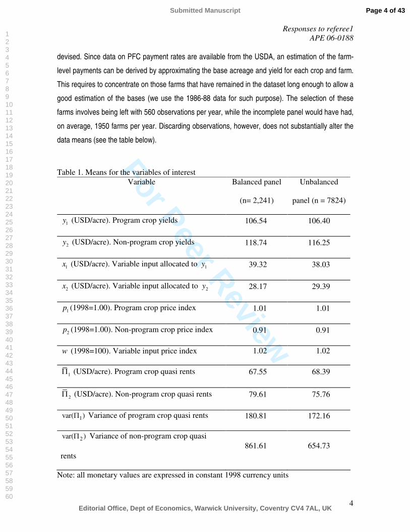
devised. Since data on PFC payment rates are available from the USDA, an estimation of the farm-

level payments can be derived by approximating the base acreage and yield for each crop and farm.

This requires to concentrate on those farms that have remained in the dataset long enough to allow a

good estimation of the bases (we use the 1986-88 data for such purpose). The selection of these

farms involves being left with 560 observations per year, while the incomplete panel would have had,

on average, 1950 farms per year. Discarding observations, however, does not substantially alter the

data means (see the table below).

Table 1. Means for the variables of interestVariable Balanced panel

(n= 2,241)

Unbalanced

panel (n = 7824)

1y (USD/acre). Program crop yields 106.54 106.40

2y (USD/acre). Non-program crop yields 118.74 116.25

1x (USD/acre). Variable input allocated to 1y 39.32 38.03

2x (USD/acre). Variable input allocated to 2y 28.17 29.39

1p (1998=1.00). Program crop price index 1.01 1.01

2p (1998=1.00). Non-program crop price index 0.91 0.91

w (1998=100). Variable input price index 1.02 1.02

1Π (USD/acre). Program crop quasi rents 67.55 68.39

2Π (USD/acre). Non-program crop quasi rents 79.61 75.76

1var( )Π Variance of program crop quasi rents 180.81 172.16

2var( )Π Variance of non-program crop quasi

rents861.61 654.73

Note: all monetary values are expressed in constant 1998 currency units

Page 4 of 43



123456789101112131415161718192021222324252627282930313233343536373839404142434445464748495051525354555657585960

For Peer Review


5

Table 1. Means for the variables of interest (continued)

Variable Balanced panel

(n= 2,241)

Unbalanced

panel (n = 7824)

1 2cov( )Π Π Quasi rents’ covariance 268.39 307.28

0W (USD). Farm’s initial wealth 669,663.10 555,070.64

1L Proportion of land allocated to 1y 0.62 0.65

2L Proportion of land allocated to 2y 0.26 0.24

3L Proportion of land left idle 0.12 0.12

A (acres). Total crop land 1075.90 1092.76


(9) (page 14) You should briefly discuss the implications of the “behavioral method."

Thanks for emphasizing the need to provide further detail of the behavioral approach which may not

be well known by readers. We have done so on page 16, where we clarify that this approach is based

upon the assumption that farmers behave as if production is characterized by constant returns to

scale with fixed input/land ratios. These fixed proportions are assumed to be based on regional

averages, though allowing for modifications for seasonal and farm-specific conditions. We also note

that the implementation of the behavioral approach requires data which are generally available (land

allocation by crop, purchases by input and sales by output). Finally, we emphasize that Just et al.

(1990) show the validity of the behavioral approach and its superiority relative to other alternative

approaches such as the profit maximization method.

(10) (page 15) Again, the role of crop rotations should be considered here.

As we explain in the response to your comment number 7, in the empirical application section, pages

17 and 18, we discuss the likely impacts of crop rotation issues on Kansas land use. We fully agree

with this referee that the implications of agronomic restrictions for land use had to be considered.

Page 5 of 43



123456789101112131415161718192021222324252627282930313233343536373839404142434445464748495051525354555657585960

For Peer Review


6

(11) (page 16) You need to provide a better definition of your variables (in Table 1). It is almost

impossible to understand the empirical specification.

Following your suggestion, table 1 now incorporates a brief definition of our variables, so that it is

easier to follow the empirical specification. Details on the units of measure of the variables are also

given.

(12) (page 16) You should also provide an explicit presentation of the exact empirical

specification that you are estimating. This should be shown in terms of the EU function.

On page 19, we offer the exact empirical specification that is estimated in our empirical application as

requested.

(13) (page 17) You refer to “market prices" here when I think you are referring to deficiency

payment supports.

Thank you for your careful review, we have substituted “market prices” by “deficiency payments.”

(14) (page 18) You should mention the role of expectations about future policy benefits as a

factor influencing production.

The role of expectations about future policy benefits has been mentioned as a factor that may

influence production. Specifically, in the concluding remarks section, we recognize the limitations of

our research and consider the analysis of the effects of expectations on land use as a possible

avenue for future research.

(15) (page 18) I do not fully understand your characterization of set-asides as “self-insurance."

This referee is right in pointing out that characterizing set-asides as a form of “self-insurance” was, at

least, confusing and we have removed the sentence from the text.

Page 6 of 43



123456789101112131415161718192021222324252627282930313233343536373839404142434445464748495051525354555657585960

For Peer Review


7

(16) (page 18) It would help your exposition to provide a simulation of policy changes on

production.

Your suggestion of including a simulation of policy changes is certainly useful. We have done so in

the last paragraph of the results section, where we simulate the impacts of the policy changes

occurred during the period studied on land use.

Again, we thank you for your useful review.

References:

Just, R.E., Zilberman, D., Hochman, E., and Bar-Shira, Z. (1990) Input Allocation in Multicrop

Systems, American Journal of Agricultural Economics, 72, 200-209.

Page 7 of 43



123456789101112131415161718192021222324252627282930313233343536373839404142434445464748495051525354555657585960

For Peer Review


TERESA SERRA, DAVID ZILBERMAN, JOSÉ M. GIL, AND

ALLEN FEATHERSTONE*

________________________________________________________________________

Abstract

The purpose of this article is to study the impact of agricultural policy decoupling on land

allocation decisions. Our analysis contributes to the literature by formally assessing the effects of

decoupling on farms’ crop mix and on the decision to set land aside. The analysis is undertaken

within the framework of the model of production under uncertainty developed by Just and

Zilberman (1986). Our empirical application focuses on a sample of Kansas farms observed from

1998 to 2001. Results show that US agricultural policy decoupling has resulted in a shift in land

use away from program crops towards non-program commodities offering higher expected profits

and idle land.


_______________________________________________________________________

Corresponding author:

Teresa Serra, CREDA-UPC-IRTA, Parc Mediterrani de la Tecnologia, Edifici ESAB, Avinguda

del Canal Olímpic s/n, 08860 Castelldefels, Spain, Phone: 34-93-552-1209, Fax: 34-93-552-

1001, e-mail: [email protected], [email protected]

* The authors are, respectively, Research Fellow at CREDA-UPC-IRTA, Parc Mediterrani de la

Tecnologia, Edifici ESAB, Avinguda del Canal Olímpic s/n, 08860 Castelldefels, Spain;

Professor at the Agricultural and Resource Economics Department, 207 Giannini Hall #3310,

University of California, Berkeley, California 94720-3310, USA; Professor at CREDA-UPC-

IRTA, Parc Mediterrani de la Tecnologia, Edifici ESAB, Avinguda del Canal Olímpic s/n, 08860

Castelldefels, Spain; Professor at the Agricultural Economics Department, 313 Waters Hall,

Kansas State University, Manhattan, Kansas 66506, USA.

Page 8 of 43



123456789101112131415161718192021222324252627282930313233343536373839404142434445464748495051525354555657585960

mailto:[email protected]

mailto:[email protected]

For Peer Review


________________________________________________________________________

Abstract

The purpose of this article is to study the impact of agricultural policy decoupling on land

allocation decisions. Our analysis contributes to the literature by formally assessing the effects of

decoupling on farms’ crop mix and on the decision to set land aside. The analysis is undertaken

within the framework of the model of production under uncertainty developed by Just and

Zilberman (1986). Our empirical application focuses on a sample of Kansas farms observed from

1998 to 2001. Results show that US agricultural policy decoupling could have involved a shift in

land use away from program crops towards non-program commodities offering higher expected

profits and idle land.


_______________________________________________________________________

Page 9 of 43



123456789101112131415161718192021222324252627282930313233343536373839404142434445464748495051525354555657585960

For Peer Review

1

I. INTRODUCTION

Until recently, the design of domestic agricultural policies in developed countries

has given priority to methods that guarantee a price floor for agricultural

commodities. Price support mechanisms can range from supply restrictions

imposed on the domestic market, price subsidies, or public purchases of

agricultural commodities to offset excess supply. A wide literature has shown

that price support mechanisms may intensify production practices and bring

about significant deadweight losses (Gardner, 1992).

The unfavourable consequences of agricultural protectionism became

widely recognized by the 1980s. It became clear that agricultural intervention

based on price guarantees and other market insulating policies led to

overproduction, which in turn brought about market distortions and

disagreements in multilateral trade policy negotiations. Recognition of these

problems motivated multilateral and/or bilateral trade agreements that advocated

for agricultural protectionism dismantling processes. In the framework of these

agreements, different countries have reformed their domestic agricultural

policies.

Economic theory views lump sum transfers as the most efficient method

to redistribute income among individuals (Williamson, 1996). The trade-off

between political pressures for continued support to farmers and the

policymakers’ will to reduce efficiency losses resulted in an increased use of

decoupled agricultural policies. Decoupling is a term used to designate the break

of the link between subsidies and production. Price supports are usually replaced

by lump sum income transfers that do not depend on current production or prices.

Page 10 of 43



123456789101112131415161718192021222324252627282930313233343536373839404142434445464748495051525354555657585960

For Peer Review

2

Several methodologies to assess the effects of agricultural policies on

farmers’ profit maximization decisions have been used. A feasible approach

consists of assuming perfect markets (including credit markets), risk neutral

producers and constant returns to scale. Under these assumptions, the literature

has shown that the impacts of decoupled policies on production decisions are

limited. However, if economic agents are not risk neutral, markets are imperfect,

or returns to scale are other than constant, apparently decoupled payments could

have more implications (see Phimister, 1995; Hennessy, 1998; or Rude, 2001). A

number of studies that have assessed economic agents’ risk preferences using

different methods have found evidence in favour of risk aversion (see, for

example, Hansen and Singleton, 1983; Chavas and Pope, 1985; Pope and Just,

1991; Abdulkadri, Langemeier and Featherstone, 2003 and 2006; or Wik et at.,

2004). In light of these findings, it has been common for policy analyses to

assume aversion to risk.1 If uncertainty and risk preferences are introduced in the

analysis of the impacts of decoupling, results suggest that apparently decoupled

policies can influence production decisions (Hennessy, 1998; Sandmo, 1971). It

is thus very important to account for risk and risk preferences when assessing the

effects of decoupling.

When coupled or partially coupled, income supports often involve

restrictive supply management rules that limit farmers’ capacity to respond to

market conditions. For example, eligibility for public subsidies is usually made 1 The role of risk has also been considered when assessing farmer decisions other than strict profit

maximization decisions. Key, Roberts and O’Donoghue (2006), for example, analyze the impacts

of risk on farm operators’ off-farm labor supply. In another line of inquiry, Abdulkadri,

Langemeier and Featherstone (2006) study the impacts of excluding risk and risk preferences on

cost structures.

Page 11 of 43



123456789101112131415161718192021222324252627282930313233343536373839404142434445464748495051525354555657585960

For Peer Review

3

conditional upon producing specific crops, the program crops. In this regard,

decoupling involves increased planting flexibility in that direct payments are not

tied to the production of certain commodities. Farmers being allowed more

planting flexibility are likely to be more responsive to market conditions and

alter their crop mix accordingly. To the extent that planting flexibility includes

the possibility of agricultural land idling, farmers will also consider setting land

aside when making their decisions on land allocation.

There are other mechanisms through which the decoupling of agricultural

policies can influence land allocation decisions. These mechanisms are the

changes in relative market prices and farmers’ risk attitudes. The reduction in

price supports is likely to make program crops less attractive relative to non-

program commodities and land idling. Also, to the extent that farmers’ risk

preferences are influenced by wealth (Sandmo, 1971; Just and Pope, 1978;

Hennessy, 1998; Just and Zilberman, 1986) and to the extent that decoupled

payments and price changes have the potential to affect the wealth of participant

farmers, their willingness to assume risk may be altered. Because risk is a

fundamental component of agricultural production and because yield variability

can differ by crop type, government transfers might affect farms’ land use by

means of altering farmers’ risk attitudes. To the extent that farmers are wealthy

and decoupled payments only represent a small proportion of their wealth,2 one

should expect small wealth effects from decoupled payments, even if farmers

display strongly decreasing absolute risk aversion.3

2 In the sample of Kansas farms utilized in the empirical application, decoupled government

payments represent less than 2% of farmers’ wealth (see the results section for more detail).

3 An anonymous Journal reviewer raised this issue.

Page 12 of 43



123456789101112131415161718192021222324252627282930313233343536373839404142434445464748495051525354555657585960

For Peer Review

4

Decoupled agricultural payments were introduced in the United States

(US) with the 1996 Federal Agricultural Improvement and Reform (FAIR) Act,

which involved a substantial change in the way income support was provided to

farmers. With the FAIR Act, market price supports and deficiency payments

were being partially replaced by Production Flexibility Contract (PFC) Payments

whose amount and entitlement would not depend on current production or prices,

and a deficiency payment program that guaranteed a minimum support price for

program crops including soybeans. Under the 1990 Act, with the exception of the

flex acres, producers were required to plant the base acreage to the base crop in

order to be eligible for deficiency payments. Entitlement to receive PFC was

based on qualified acres historically enrolled in commodity programs, allowing

land to be put to any agricultural use, including the production of any crop with

the exception of fruits and vegetables (unless it was used in this way in the past),

or idled.

The purpose of this article is to study the impacts of decoupling on land

allocation decisions. Our analysis contributes to the literature by formally

assessing the effects of decoupling on farms’ crop mix and on the decision to set

land aside. The analysis is undertaken within the framework of a model of

production under uncertainty developed by Just and Zilberman (1986). We

extend this model to study supply responses to decoupled payments and to

include set aside among land use alternatives. Though various analyses have

addressed the effects of decoupling on producers’ decisions, no existing research

has studied the impacts of decoupled payments on farms’ land allocation using

the extended Just and Zilberman (1986) model. Our empirical application

focuses on a sample of Kansas farms observed from 1998 to 2001. Results

Page 13 of 43



123456789101112131415161718192021222324252627282930313233343536373839404142434445464748495051525354555657585960

For Peer Review

5

suggest that US agricultural policy decoupling may result in a shift in land use

away from program crops towards non-program commodities offering higher

expected profits and idle land.

II. CONCEPTUAL FRAMEWORK

The objective of our model is to assess the effects of decoupling on farm land

allocation. We adopt the Just and Zilberman (1986) model of production under

uncertainty. Because agricultural producers are not likely to be neutral to risk,

farmers’ risk preferences are explicitly considered. Our model defines risk

preferences as a function of wealth (Just and Zilberman, 1986; Pope and Just,

1991; Hennessy, 1998). If economic agents are risk averse and their risk aversion

decreases with wealth (Pope and Just, 1991; Bar-Shira, Just and Zilberman,

1997), an increase in decoupled payments is expected to alter the crop mix

towards more risky crops that offer higher expected margins. The reduction in

price supports for program crops that characterizes a decoupling process will

reduce the attractiveness of these crops in favour of non-program commodities

and/or idle land. Apart from the substitution effects, a change in output prices

will also have an income effect that, under the assumption of decreasing absolute

risk averse (DARA) preferences, is likely to increase risk aversion.

The 1996 FAIR Act involved the introduction of decoupled payments that

allowed, with some restrictions, full planting flexibility. We extend the Just and

Zilberman (1986) model to allow for these payments and the possibility to

receive them even if agricultural land is left idle. Our model offers an improved

Page 14 of 43



123456789101112131415161718192021222324252627282930313233343536373839404142434445464748495051525354555657585960

For Peer Review

6

picture of farmers’ behaviour by re-optimizing land allocation in response to

policy. We model PFC payments as simple lump sum transfers, thus recognizing

that under the new scenario farmers manage their crop mix in accordance with

market conditions.

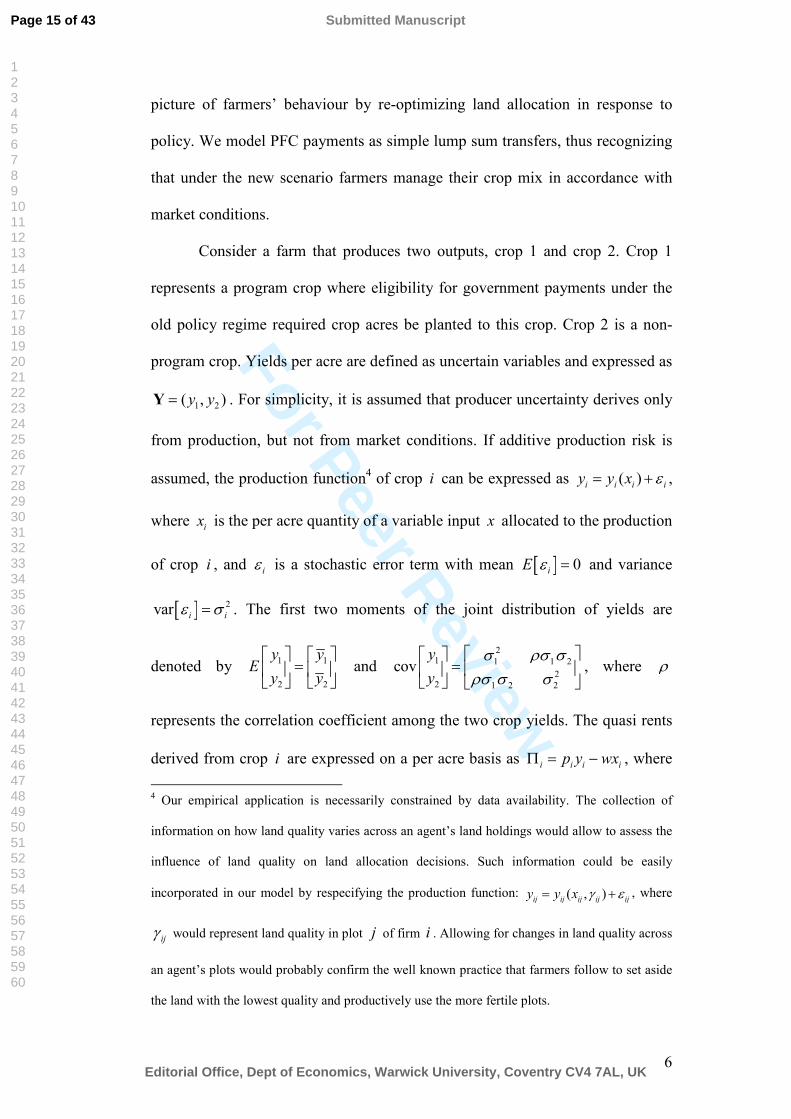
Consider a farm that produces two outputs, crop 1 and crop 2. Crop 1

represents a program crop where eligibility for government payments under the

old policy regime required crop acres be planted to this crop. Crop 2 is a non-

program crop. Yields per acre are defined as uncertain variables and expressed as

1 2( , )y y=Y . For simplicity, it is assumed that producer uncertainty derives only

from production, but not from market conditions. If additive production risk is

assumed, the production function4 of crop i can be expressed as ( )i i i iy y x ε= + ,

where ix is the per acre quantity of a variable input x allocated to the production

of crop i , and iε is a stochastic error term with mean [ ] 0iE ε = and variance

[ ] 2var i iε σ= . The first two moments of the joint distribution of yields are

denoted by 1 1

2 2

y yE

y y

=

and 2

1 1 1 22

2 1 2 2

covyy

σ ρσ σρσ σ σ

=

, where ρ

represents the correlation coefficient among the two crop yields. The quasi rents

derived from crop i are expressed on a per acre basis as i i i ip y wxΠ = − , where 4 Our empirical application is necessarily constrained by data availability. The collection of

information on how land quality varies across an agent’s land holdings would allow to assess the

influence of land quality on land allocation decisions. Such information could be easily

incorporated in our model by respecifying the production function: ( , )ij ij ij ij ijy y x γ ε= + , where

ijγ would represent land quality in plot j of firm i . Allowing for changes in land quality across

an agent’s plots would probably confirm the well known practice that farmers follow to set aside

the land with the lowest quality and productively use the more fertile plots.

Page 15 of 43



123456789101112131415161718192021222324252627282930313233343536373839404142434445464748495051525354555657585960

For Peer Review

7

ip represents crop i price and w is the variable input price, being the first two

moments of the joint distribution of quasi rents 1 1

2 2

EΠ Π

= Π Π and

21 1 1 2

22 1 2 2

covϖ ρϖ ϖ

ρϖ ϖ ϖΠ

= Π , where i i ipϖ σ= .

Total crop land ( )A 5 is allocated to the production of the two crops

considered or left idle6 yielding the following vector of land allocation:

( )1 2 3, ,A A A=A , where 1 2 3A A A A= + + , 3A represents idle land and 1A and 2A

symbolize land allocated to program and non-program crops respectively. The

problem of land allocation can alternatively be expressed in proportions as

( )1 2 3, ,L L L=L , where ii

ALA

= and 1 2 3 1+ + =L L L .

It is assumed that farmers make their decisions with the aim of

maximizing the expected utility of their wealth [ ]1 2 3 1 2, , , ,

max ( )L L L x x

E u W =

( )1 3 1 2

0 1 1 2 1 3, , ,max (1 )+ +Π +Π − − L L x x

E u W G AL A L L , where W represents farms’ total

wealth, 0W stands for farms’ initial wealth, and G are decoupled income-support

payments. The quasi rent associated to idle land is assumed to be equal to zero.

5 Because, for our sample of farms, crop land remained almost constant during the period of

analysis, A is assumed to be fixed.

6 The Conservation Reserve Program (CRP) does not factor into the land idling consideration of

this paper. Since it consists of long-term contracts that promote the establishment of conserving

covers on environmentally sensitive cropland, it precludes adapting land use to changing market

conditions or policy regulations.

Page 16 of 43



123456789101112131415161718192021222324252627282930313233343536373839404142434445464748495051525354555657585960

For Peer Review

8

Following previous literature, we assume risk neutrality in the input decision7

which leads to independence of land allocation from variable input decisions

(Just and Zilberman, 1986). Under this assumption the first order conditions of

the land allocation problem can be expressed as:

[ ] ( )1 21

0∂ ∂ = Π −Π ≥ ∂ ∂

E u uEL W

(1.1)

[ ] ( )23

0∂ ∂ = −Π ≥ ∂ ∂

E u uEL W

(1.2)

By approximating the marginal utility around the expected wealth

( )0 1 1 2 1 3(1 )= + +Π +Π − −W W G AL A L L through a second-order Taylor series

expansion, the first order conditions can be alternatively expressed as:

( ) { }1 21 1 3 2(1 ) 0ν ν

Π −Π− + − ≥R L L

A(2.1)

{ }21 2 3 3( ) (1 ) 0ν ν−Π

− − + − ≥R L LA

(2.2)

where 12

2( )− ∂ ∂ = = − ∂ ∂

u uR R WW W

represents the Arrow-Pratt coefficient of

absolute risk aversion. Following Bar-Shira, Just and Zilberman (1997) we

7 As Just and Zilberman note, the assumption of risk neutrality is very common in models with

stochastic production and is necessary for the dual cost and production functions to be

independent of risk preferences. This assumption allows to derive a theoretical framework that is

more tractable at the empirical level.

Page 17 of 43



123456789101112131415161718192021222324252627282930313233343536373839404142434445464748495051525354555657585960

For Peer Review

9

assume R to be a function of farms’ expected wealth that can be represented by

R W βη= , where η and β are parameters that represent a farmer’s risk

preferences. This is a flexible specification in that it does not restrict the specific

type of farmers’ risk preferences. Risk averse (neutral) [seeking] attitudes are

represented by ( )[ ]0η > = < . We assume farmers to be risk-averse ( > 0η ). The

wealth elasticity of absolute risk aversion corresponds to β . If farmers have

decreasing (constant) [increasing] absolute risk aversion preferences,

( )[ ]0β > = < . In accord with previous studies (Bar-Shira, Just and Zilberman,

1997; Isik and Khanna, 2003; Eisenhauer and Ventura, 2003) we assume here

that farmers have DARA preferences ( < 0β ). The expression

1 =v 2 21 1 2 22ϖ ρϖ ϖ ϖ− +

1

var 0T

L ∂Π

= > ∂ is the variance of the marginal profit

derived from increasing land allocated to crop 1i = and

1 1 1 3 2(1 )Π = Π + − − ΠT L L L . The result of multiplying 2v 21 2 2ρϖ ϖ ϖ= − by

3(1 )− L is 1

var12∂ Π∂

T

L, which represents one-half the marginal variance of profit

when 1 0L = , i.e. at zero capacity allocation. Finally, 23 2ϖ= −v corresponds to

the negative value of the variance of non-program crop quasi rents. Note that

expressions (2.1) and (2.2) above involve the equalization of the marginal mean

income effect derived from an increase in land allocated to crop i and the

marginal risk effect discounted to a certainty equivalent using the Arrow-Pratt

coefficient of absolute risk aversion.

In order to determine the effects of decoupling on land allocation

decisions, we use comparative statics. The consideration of a multi-product land

allocation problem involves substantial complexity relative to a more simplified

Page 18 of 43



123456789101112131415161718192021222324252627282930313233343536373839404142434445464748495051525354555657585960

For Peer Review

10

two-product model and yields comparative statics formulae that cannot be

signed. In order to make comparative statics more simple, but also more clear,

we simplify the model to a consideration of only two alternatives in the land

allocation problem: 1L and iL , 2,3i = .8 It is important to note that model

simplification is only limited to the comparative statics analysis in this section,

and that the empirical implementation will be based upon the generalized three-

product model.

Crop rotation issues might be relevant and represent a factor affecting

land use decisions other than economic and political reasons.9 Crop rotation is a

reason for diversification and affects the relative profitability of a crop at a given

field because of soil dynamics. Farmers being aware of this, can establish

constraints on land use patterns. Crop rotation can occur between program crops

or between program and non-program crops. Since program crops are grouped

under a single output category, only the inter-group rotation would affect our

results. Unfortunately, our database does not contain information on agronomic

issues. As a result, crop rotation cannot be explicitly modelled, though it is

implicitly accounted for. Were data available, agronomic restrictions could easily

be introduced in the model by solving a constrained optimization problem. It is

also true however, that rotation constraints did not change with policy reforms

and, from this perspective, the effects of not explicitly modelling crop rotation

should not be very relevant for our policy analysis.

8 Note that this simplification is economically reasonable as it represents two possible corner

solutions that can apply to our problem, i.e. that farmers decide not to set land aside or diversify

the crop mix.

9 This was suggested by an anonymous Journal reviewer.

Page 19 of 43



123456789101112131415161718192021222324252627282930313233343536373839404142434445464748495051525354555657585960

For Peer Review

11

The value of crop rotation might have changed with policy reforms. On

the one hand, pre-reform coupled payments to program crops not allowing to put

land to other agricultural uses, are very likely to have reduced the value of

rotating non-program with program commodities. With the decoupling of

payments and the allowance of planting flexibility, farmers are likely to have

been more willing to rotate program with non-program commodities. On the

other hand, however, the reform-induced reduction in price supports to program

crops is likely to have cut down the value of planting non-program crops for

rotation purposes. This is because any extra yields in program crops obtained as a

result of rotation will now have a lower market value. As a result, the overall

impact of crop rotation is not very likely to have been relevant. A discussion of

the consequences of crop rotation for land use in Kansas is offered in the

empirical application section.

Let’s consider a land allocation problem that only includes program and

non-program commodities. In such a scenario, the system of first-order

conditions is reduced to:

( ) { }1 21 1 2 0ν ν

Π −Π− + =R L

A(3)

where 11

varν ∂Π

= ∂ T

L, 2

1

var12

ν ∂ Π=

∂T

L, and 1 1 1 2(1 )Π = Π + − ΠT L L . As

explained above, in a decoupling process lump sum payments are usually

introduced to replace price supports. Our comparative statics analysis thus

focuses on determining the sensitivity of the crop mix to changes to program

Page 20 of 43



123456789101112131415161718192021222324252627282930313233343536373839404142434445464748495051525354555657585960

For Peer Review

12

crop prices and to lump sum payments. The comparative statics results can be

summarized in the following propositions (proofs are presented in the appendix).

PROPOSITION 1. Land allocated to the program crop ( = 1i ) increases with an

increase in decoupled payments (G ) if 2

1

ϖρϖ

> , or if 2

1

ϖρϖ

−∞ < < and

1 1 2ν ν>L . On the other hand, land allocated to the program crop decreases

with an increase in G if 2

1

ϖρϖ

−∞ < < and 1 1 2ν ν<L .

Proposition 1 can be economically interpreted as follows. An increase in

decoupled payments improves farmers’ wealth which in turn increases their

willingness to assume more risk. This could reduce the attractiveness of crop mix

diversification as a strategy to manage farm income risk. This will only occur if

yield correlation is negative or takes low positive values, and if an increase in

program crop production substantially reduces the profit ( TΠ ) variance.

Otherwise diversification will not be pursued.

PROPOSITION 2. For a negative value of the mean effect of production, land

allocated to the program crop decreases with an increase in 1p if 0ρ < and

1 21

1 1

ν ν∂ ∂>

∂ ∂L

p p, if 1

2

0 ϖρϖ

< < , or if 1

2

ϖρϖ

> and 1 21

1 1

ν ν∂ ∂<

∂ ∂L

p p. Otherwise,

land allocated to crop 1 only decreases if the mean effect outweighs the risk

effect.

Page 21 of 43



123456789101112131415161718192021222324252627282930313233343536373839404142434445464748495051525354555657585960

For Peer Review

13

The economic meaning of proposition 2 can be expressed as follows. If the

expected mean effect of production is negative, an increase in 1p only motivates

an increase in 1L if this increase involves some gains in terms of risk

management that outweigh the negative mean effect. If yields are negatively

correlated, the gains in terms of risk management require a substantial reduction

in the marginal variance of profit. However, if yields are highly and positively

correlated (and thus diversification towards 2L is less attractive) a small increase

in the marginal variance is tolerated, as long as the risk effect is of bigger

magnitude than the mean effect.

PROPOSITION 3. For a positive value of the mean effect of production, land

allocated to the program crop increases with an increase in 1p if 0ρ < and

1 21

1 1

ν ν∂ ∂<

∂ ∂L

p p, or if 1

2

ϖρϖ

> and 1 21

1 1

ν ν∂ ∂>

∂ ∂L

p p. Otherwise, land allocated to

crop 1 only increases if the mean effect outweighs the risk effect.

Proposition 3 thus shows that, because the expected mean effect is positive, no

diversification in favour of non-program crops is pursued if yield correlation is

high and positive. However, if 0ρ < an increase in 1L requires an important

reduction in the marginal variance of profit.

In order to assess the effects of decoupling on idle land, we now consider

a model that examines the allocation of land among program crop production and

set aside. In such a model, the first order condition in (3) changes to (4) below:

Page 22 of 43



123456789101112131415161718192021222324252627282930313233343536373839404142434445464748495051525354555657585960

For Peer Review

14

211 1 0ϖΠ

− =RLA

(4)

Comparative statics allow to formulate the following two propositions:

PROPOSITION 4. Idle land is reduced with an increase in decoupled payments.

This is due to the fact that an increase in decoupled payments reduces farmers’

degree of risk aversion increasing their willingness to assume more risk. Given

that idle land involves no risk, this alternative becomes less attractive in favour

of producing agricultural commodities.

PROPOSITION 5. For a negative value of the mean effect of production, idle

land increases with an increase in 1p to the detriment of 1L . However, if the

mean effect of production is positive, idle land only increases if the risk effect

outweighs the mean effect.

In a situation where the mean effect of production is positive, farmers have the

incentive to increase the amount of land allocated to program crops to the

detriment of idle land, as long as the increase in production risk measured as a

certainty equivalent does not outweigh the mean effect. However, if the mean

effect is negative, an increase in 1p reduces program crop land in favour of idle

land.

In summary, our comparative statics analysis shows that decoupled

payments have the effect of reducing idle land. In contrast, the reduction in

Page 23 of 43



123456789101112131415161718192021222324252627282930313233343536373839404142434445464748495051525354555657585960

For Peer Review

15

program crop price supports can motivate land set aside. Decoupled payments

can also stimulate a change in crop mix in favour of non-program commodities.

This shift requires yield correlation to be negative or take low positive values. A

decrease in program crop price supports can also boost non-program crops

acreage under certain conditions. It is relevant to note that, with the exception of

the influence of decoupled payments on idle land, the net effects of decoupling

depend on issues such as yield correlation, changes in the variance of profit, or

the magnitude of the mean and risk production effects. This causes the response

to a decoupled program to be inconclusive making it necessary to determine it

empirically.

III. EMPIRICAL APPLICATION

As explained above, our empirical application is focused on the analysis of the

effects of the US agricultural policy reforms in 1996 on land allocation decisions

made by a sample of Kansas farms. Specifically, we are interested in observing

how the planting flexibility provisions and the decoupling of farm income

support influenced Kansas farms’ land use.

Farm-level data are taken from farm account records from the Kansas

Farm Management Association database for the period 1998 to 2001.

Retrospective data for these farms are also used to define some lagged variables

used in the application.10 The Kansas Farm Management Association database

collects information from individual farms on an annual basis through a

10 To be able to do so, a complete panel of data is built out of our sample.

Page 24 of 43



123456789101112131415161718192021222324252627282930313233343536373839404142434445464748495051525354555657585960

For Peer Review

16

cooperative record-sharing, farm management, and tax preparation arrangement.

Around 2,500 full-time commercial holdings with gross sales exceeding

$100,000 provide data to this database. Various farm types and areas in Kansas

are represented in the dataset (Albright, 2001). The variables in the database

include, among other information, farm financial and production data, balance

sheet, cash flow and income statements. Our analysis is based on farm-level data,

but aggregates are also used to define important variables that are unavailable in

the farm-level dataset. These aggregates are taken from the United States

Department of Agriculture (USDA) and the National Agricultural Statistics

Service (NASS). USDA provided state-level PFC payment rates and NASS

facilitated country-level price indices and state-level output prices and quantities.

Table 1 contains summary statistics for the variables used in the analysis.

Following our model specification, we consider a variable input x that includes

the per acre application of herbicides and fertilizer, representing the main

variable costs for the farms in the sample. Because input prices are not available

from the Kansas database, we define w as a country-level input price index.

Variable x is then defined as an implicit quantity index and derived through the

ratio of input use in currency units to the corresponding price index. The Kansas

dataset does not provide information on the consumption of variable inputs by

crop. We use Just et al. (1990) behavioural proposal to allocate variable input use

among different crops. The behavioral approach is based upon the assumption

that farmers behave as if their production functions are characterized by constant

returns to scale with fixed input/land ratios. Allowing for modifications for

seasonal and farm-specific conditions, these fixed proportions are assumed to be

based on regional averages. The only necessary data for implementing this

Page 25 of 43



123456789101112131415161718192021222324252627282930313233343536373839404142434445464748495051525354555657585960

For Peer Review

17

procedure are records on land allocation by crop, purchases by input and sales by

output. Just et al. (1990) show the validity of the behavioral approach and its

superiority to other alternative approaches.11

Two output categories are distinguished as quantity indices per acre ( 1y

and 2y ). Variable 1y represents program crops and includes the production of

wheat, corn, and grain sorghum per acre. Variable 2y is the production of

soybeans representing a non-program commodity. Together, wheat, corn,

sorghum and soybeans represent the main crops in Kansas. Paasche indices for

both crops are computed using state-level output prices and production to define

1p and 2p .

Crop rotation, which we do not observe, is a relevant practice in Kansas

with much benefit from using program crops in rotation with non-program crops.

As explained above, apart from economic and policy issues, land use can also be

affected by crop rotation. According to Dumler and Duncan (2005)12 the passage

of the 1996 FAIR Act may have favored rotation of program with non-program

crops such as soybeans, without losing program payments. From this perspective,

rotation issues would be an added reason to switch from program crops to

soybeans or idle land. However, as noted above, the value of rotating non-

program with program crops may have been reduced with the decline in program

crop prices. In other words, any increase in soybeans production is more likely to

11 We should note here that another allocation mechanism based on profit maximization was also

used, but yielded inconsistent results. This is not surprising in light of Just et al. (1990) findings

that the behavioural method is superior.

12 Halloran (2006), on the other hand, finds that for potato cropping systems, rotating program

with non-program crops can improve economic viability and reduce risk.

Page 26 of 43



123456789101112131415161718192021222324252627282930313233343536373839404142434445464748495051525354555657585960

For Peer Review

18

have been driven by a change in relative market prices than by agronomic

reasons. As a result, the overall impacts are not likely to have been very relevant.

iA represents land allocated to alternative 1,2i = ,3, with A representing

total crop acres, 3A the acres left idle, and 1A and 2A the crop acres planted to

program and non-program crops respectively. By using iy , ix , ip , w , the value

for iΠ can be determined. Computing quasi rents at the farm-level involves

some problems. First, not every farm produces crop i 13 every year and when this

happens iΠ cannot be determined at the farm-level. Second, the composition of

1y can vary annually within a farm as land planted to wheat, corn and sorghum

changes, which complicates the definition of a reasonable value for 1Π at the

farm-level. In light of these problems, we define quasi rents using annual sample-

means for the production and input consumption variables.14

Kansas database does not register PFC government payments. Instead, a

single measure including all government payments received by each farm is

available. To derive an estimate of farm-level PFC payments, the acreage of

program crops (base acreage) and the base yield for each crop are approximated

using farm-level data. The approximation uses the 1986-88 average acreage and

yield for each program crop and farm. PFC payments per crop are derived by

13 The problem applies to crop 2i = .

14 It is important to note here that other alternatives were also considered, including the use of

farm-level iΠ values whenever possible (and averages otherwise), or the use of the Kansas

Farm Management Association crop budgets (http://www.agmanager.info/crops/). However,

these alternatives yielded results in contrast to widely accepted previous research results and thus

were discarded.

Page 27 of 43



123456789101112131415161718192021222324252627282930313233343536373839404142434445464748495051525354555657585960

For Peer Review

19

multiplying 0.85 by the base acreage, yield, and the PFC payment rate. PFC

payments per crop are then added to get total direct payments per farm.15 A

farm’s initial wealth is defined as the farm’s net worth.

In order to achieve the aforementioned objectives, the following system

of first-order conditions is estimated using two-stage nonlinear least squares:

( ) ( ){ }( )1 21 1 2 1 2 3 1 2 2var( ) var( ) 2cov( , ) (1 ) cov( , ) var( ) 0W L L

Aβη

Π −Π− Π + Π − Π Π + − Π Π − Π =

(5.1)

( ) ( ){ }21 1 2 2 3 2cov( , ) var( ) (1 ) var( ) 0W L L

Aβη−Π

− − Π Π + Π − − Π = (5.2)

IV. RESULTS

Table 1 shows that, during the period studied, more than 62% of crop land was

planted to program crops, 26% was devoted to non-program commodities, and

12% was left idle. Sample means also show that estimated PFC payments

represent around 1.8% of farmers’ initial wealth. Of interest is the fact that, for

the period of analysis, the expected market profit per acre derived from non-

program commodities outweighs the one obtained from program crops. Also,

during the period of study, 2 1var var( ) ( )Π > Π , which involves higher income risk

15 This estimate is compared to actual government payments received by each farm. If estimated

PFC payments exceed actual payments, the first measure is replaced by the second.

Page 28 of 43



123456789101112131415161718192021222324252627282930313233343536373839404142434445464748495051525354555657585960

For Peer Review

20

derived from non-program crops.16 Two-stage nonlinear least squares parameter

estimates for the system of first-order conditions (see table 2) provide evidence

that farmers in our sample are risk averse, and that the degree of risk aversion

decreases with farmers’ wealth, i.e., farmers exhibit DARA preferences.

Price, cross-price and payment elasticities of the proportion of land

planted to program and non-program crops or left idle are presented in table 3.

As expected, results suggest that an increase in its own price increases the

quantity of land planted to program crops. Quite the opposite, the price elasticity

of non-program crops is negative. This result is not surprising given the high

income risk associated with 2y during the period of analysis. An increase in 2p

does not only involve an increase in mean income, but also a substantial increase

in income variance. This lays out the necessary conditions for a failure in the

‘law of supply’, that contends that the quantity supplied by price-taking

producers will rise in response to an increase in output prices. An increase in

profit risk above the increase in its mean will originate this failure. This result is

in accord with the findings of Just and Zilberman (1986). Results indicate that

cross-price effects are negative for program crop and positive for non-program

crop prices. Hence, a decline in program crop deficiency payments motivates a

change in land use away from program crops in favour of non-program

commodities. In contrast, farmers will respond to an increase in non-program

crop prices by increasing land devoted to other uses such as program crops. The

response of idle land to changes to market prices is quite different depending on

whether it is the program or the non-program crop price that is changed. An 16 Differences in the variance of profits might partly reflect the fact that 1y is a composite output,

and 2y is a single crop.

Page 29 of 43



123456789101112131415161718192021222324252627282930313233343536373839404142434445464748495051525354555657585960

For Peer Review

21

increase in program crop prices creates a strong incentive to reduce idle land to

plant program commodities.17 This shift in land use takes place because the

increase in mean income originated by the increase in 1p outweighs the increase

in income risk. However, an increase in 2p does not reduce idle land. Instead

idle acreage is increased. As noted before, the high risk associated to the

production of 2y for the period studied is increased with an increase in the output

price. The relevance of the risk effect relative to the mean effect motivates

farmers to set some land aside. Land use is also sensitive to government

subsidies. An increase in decoupled payments reduces farmers’ degree of risk

aversion and stimulates undertaking risky activities. This involves a reduction in

idle land in favour of crop land planted to both program and non-program

commodities.

Hence, our results show that agricultural policy decoupling is likely to

have motivated a change in farmers’ crop mix. The extremely low values of

subsidy elasticities relative to price elasticities allow to predict a reduction in the

acreage planted to program crops in favour of non-program commodities and idle

land. In order to better show the utility of our model, we carry out a simulation

exercise that assesses the effects of shocking the model in accordance with the

policy changes occurred during the period studied. During this period, marketing

assistance loan rates declined approximately by 6.4%, while deficiency payments

were cut by almost 29%. We assume the reduction in marketing assistance loan

rates to be fully incorporated into the output prices received by farmers. As a

result of the decline in program crop prices, our simulations suggest a reduction

in program crop land on the order of 12% in favour of non-program crops, that 17 High idle land elasticities are partly due to the low initial values of this variable.

Page 30 of 43



123456789101112131415161718192021222324252627282930313233343536373839404142434445464748495051525354555657585960

For Peer Review

22

increase their area by 13%, and idle land, that is augmented by 35%. The low

elasticity values of decoupled payments involve small changes in land allocation

as a result of a change in PFC payments. Both program and non-program crop

acres increase by less than 0.2%, while idle land is reduced by 1.3%. As a result

of these changes, the new land allocation vector at the data means is 1 0.55L = ,

2 0.29L = , and 3 0.16L = .

V. CONCLUDING REMARKS

This paper investigates the effects of decoupling on farmers’ land allocation

decisions and, specifically, on the crop mix and idle land. Coupled policies

usually restrict farmers’ capacity to respond to market conditions by imposing

restrictive supply management rules. In this regard, decoupling involves

increased planting flexibility and thus may motivate changes in land allocation.

Other aspects of decoupling can also influence land allocation decisions. These

aspects are the reduction in price supports for program crops and their

replacement by lump sum transfers, which are likely to involve changes in

relative market prices and in farmers’ risk attitudes.

In order to show how these policy reforms could affect land use, we use

an extended version of the Just and Zilberman (1986) model of production under

uncertainty. Our model offers an improved picture of farmers’ behaviour by

allowing to optimize land allocation in response to policy and by considering

land idling among land use alternatives. Theoretical results show that, under the

assumption of DARA preferences, an increase in lump sum transfers will

Page 31 of 43



123456789101112131415161718192021222324252627282930313233343536373839404142434445464748495051525354555657585960

For Peer Review

23

increase farmers’ willingness to assume more risk. This could reduce the

attractiveness of crop mix diversification away from program crops and in favour

of non-program commodities as a strategy to manage farm income risk. This

involves that this diversification will only be pursued if yield correlation between

program and non-program crops is negative or takes low positive values, and if

an increase in land allocated to program crops involves a substantial reduction in

the profit variance. Under certain conditions of yield correlation, profit variance

and mean income, a decrease in program crop price supports will motivate

diversification away from these crops. Idle land will decrease as a result of a

reduction in program crop prices, only if the mean effect of production is

negative or if it is positive and the risk effect outweighs the mean effect. An

increase in decoupled subsidies will motivate farmers to assume riskier

enterprises and reduce uncultivated land.

We use farm-level data collected in Kansas to illustrate our model and

determine the effects of the FAIR Act on crop mix diversification. Our results

show that decoupling may induce a change in farmers’ crop mix by stimulating

to reduce program crop acres in favour of non-program commodities and land

idling.

Our work represents a first step in the analysis of the impacts of

decoupling on land allocation. Our empirical analysis is however constrained by

data availability. Due to data restrictions, we are not able to assess the role of

agronomic restrictions such as crop rotation issues on land use, which constitutes

a promising extension of our work. Another future line of inquiry would involve

the consideration of the influence of land quality on land allocation decisions.

The collection of data on farmers’ expectations about future policy benefits

Page 32 of 43



123456789101112131415161718192021222324252627282930313233343536373839404142434445464748495051525354555657585960

For Peer Review

24

would allow an evaluation of the effects of policy expectations on land use and

constitutes another possible extension of our analysis.

Page 33 of 43



123456789101112131415161718192021222324252627282930313233343536373839404142434445464748495051525354555657585960

For Peer Review

25

APPENDIX

Proof of proposition 1. By totally differentiating equation (3), the following

expression can be derived:

[ ]11 1 2

1 ν ν∂ ∂= − +

∂ ∂L R LG D W

(6)

where 0D > is the negative value of the second order condition of the

optimization problem. If crop yields are negatively correlated (i.e. 0ρ < ),

2 0ν < , which involves that 1 0∂>

∂LG

if 1 1 2ν ν>L . If the correlation coefficient

is positive (i.e. 0ρ > ), 2 ( )0ν > < if 2

1

( )ϖρϖ

> < . We can thus conclude that if

2

1

0 ϖρϖ

< < and 1 1 2( )ν ν> <L , then 1 ( )0LG∂

> <∂

. Otherwise, if 2

1

ϖρϖ

> , land

allocated to program crops will increase with an increase in decoupled payments

1 0LG∂ > ∂

.



( )1 1 21 1 1 21_

1 1 1

1 ν νε Π −Π ∂ ∂ ∂

= − − + ∂ ∂ ∂ R W

LL y R Lp D A W D p p

(7)

Page 34 of 43



123456789101112131415161718192021222324252627282930313233343536373839404142434445464748495051525354555657585960

For Peer Review

26

where ( )1 1 2

1 _1 ε Π −Π

−

R W

Ly

A W represents the mean effect of production per

unit of land, being 1 21

1 1

ν ν ∂ ∂+ ∂ ∂

R Lp p

the variance effect discounted to a

certainty equivalent using the Arrow-Pratt coefficient of absolute risk aversion.

Expression 1

1

ν∂∂p

represents the marginal variance of the marginal profit, and

2

1

ν∂∂p

stands for a half of the change in the marginal variance of profit when

1 0L = . The elasticity _ 0R WR WW R

ε ∂= <∂

represents the wealth elasticity of the

Arrow-Pratt coefficient of absolute risk aversion.

If yield correlation coefficient is negative ( 0ρ < ), then 1

1

0ν∂>

∂pand

2

1

0ν∂<

∂p, i.e., the variance of the marginal profit increases, but the marginal

variance of profit decreases. In such a situation, the sign of the marginal risk

effect is positive if 1 21

1 1

ν ν∂ ∂>

∂ ∂L

p pwhich involves 1

1

0∂<

∂Lp

. Otherwise, the

marginal effect is negative and the sign of 1

1

Lp∂∂

depends on the magnitude of the

mean effect relative to the marginal effect. If yield correlation is positive, then

1

1

( )0ν∂> <

∂pif 1

2

( )ϖρϖ

< > and 2

1

0ν∂>

∂p. This involves that if 1

2

ϖρϖ

> and

1 21

1 1

ν ν∂ ∂<

∂ ∂L

p p, or if 1

2

0 ϖρϖ

< < , then 1

1

0Lp∂

<∂

.

Proof of proposition 3. See proof of proposition 2.

Page 35 of 43



123456789101112131415161718192021222324252627282930313233343536373839404142434445464748495051525354555657585960

For Peer Review

27



21 1 1 0ϖ∂ ∂= − >

∂ ∂L L RG D W

(8)



21 1 1 11 1 1

1

1 2RdL y L R L pdp D A W D

ε σ Π = − − (9)

Page 36 of 43



123456789101112131415161718192021222324252627282930313233343536373839404142434445464748495051525354555657585960

For Peer Review

28

REFERENCES

Abdulkadri, A. O., Langemeier, M. R., and Featherstone, A. M. (2003)

Estimating Risk Aversion Coefficients for Dryland Wheat, Irrigated Corn

and Dairy Producers in Kansas, Applied Economics, 35, 825-834.

Abdulkadri, A. O., Langemeier, M. R., and Featherstone, A. M. (2006)

Estimating Economies of Scope and Scale Under Price Risk and Risk

Aversion, Applied Economics, 38, 191-201.

Albright, M. L. (2001) Kansas Agriculture: An Economic Overview for 2001.

Kansas State Research and Extension, Research Papers and Presentations,

Manhattan, Kansas (available at

http://www.agmanager.info/farmmgt/income/papers/

KSAgEconomy2001.pdf).

Bar-Shira, Z., R.E. Just, and Zilberman, D. (1997) Estimation of Farmers’ Risk

Attitude: An Econometric Approach, Agricultural Economics, 17, 211-

222.

Chavas, J.P. and Pope, R.D. (1985) Price Uncertainty and Competitive Firm

Behavior: Testable Hypotheses from Expected Utility, Journal of

Economics and Business, 37, 223-235.

Dumler, T. and Duncan, S. R. (2005) Wheat Cost-Return Budget in North

Central Kansas. Kansas State Research and Extension, Farm Management

Guide MF-2158, Manhattan, Kansas (available at

http://www.oznet.ksu.edu/library/agec2/mf2158.pdf).

Eisenhauer, J. G. and Ventura, L. (2003) Survey Measures of Risk Aversion and

Prudence, Applied Economics, 35, 1477-1484.

Page 37 of 43



123456789101112131415161718192021222324252627282930313233343536373839404142434445464748495051525354555657585960

http://www.oznet.ksu.edu/library/agec2/mf2158.pdf

http://www.agmanager.info/farmmgt/income/papers/

For Peer Review

29

Gardner, B.L. (1992) Changing Economic Perspectives on the Farm Problem,

Journal of Economic Literature, 30, 62-101.

Halloran, J. (2006) The 2002 Farm Bill Commodity Programs: A Tool for

Improving Rotation Crop Profitability and Reducing Risk in Potato

Cropping Systems, Applied Economics Letters, 13, 171-175.

Hansen, L. and Singleton, K. (1983) Stochastic Consumption, Risk Aversion, and

the Temporal Behavior of Asset Returns, Journal of Political Economy,

91, 249-265.

Hennessy, D.A. (1998) The Production Effects of Agricultural Income Support

Policies Under Uncertainty, American Journal of Agricultural

Economics, 80, 46-57.

Isik, M. and Khanna, M. (2003) Stochastic Technology, Risk Preferences, and

Adoption of Site-Specific Technologies, American Journal of

Agricultural Economics, 85, 305-317.

Just, R.E. and Pope, R.D. (1978) Stochastic Specification of Production

Functions and Economic Implications, Journal of Econometrics, 7, 67-86.

Just, R.E. and Zilberman, D. (1986) Does the Law of Supply Hold Under

Uncertainty, The Economic Journal, 96, 514-524.

Just, R.E., Zilberman, D., Hochman, E., and Bar-Shira, Z. (1990) Input

Allocation in Multicrop Systems, American Journal of Agricultural

Economics, 72, 200-209.

Key, N., Roberts, M. J., and O’Donoghue, E. (2006) Risk and Farm Operator

Labour Supply, Applied Economics, 38, 573-586.

Page 38 of 43



123456789101112131415161718192021222324252627282930313233343536373839404142434445464748495051525354555657585960

For Peer Review

30

Phimister, E. (1995) Farm Household Production in the Presence of Restrictions

on Debt: Theory and Policy Implications, Journal of Agricultural

Economics, 46, 371-380.

Pope, R.D., and Just, R.E. (1991) On Testing the Structure of Risk Preferences in

Agricultural Supply Analysis, American Journal of Agricultural

Economics, 73, 743-748.

Rude, J.I. (2001) Under the Green Box. The WTO and Farm Subsidies, Journal

of World Trade, 35, 1015-1033.

Sandmo, A. (1971) On the Theory of the Competitive Firm Under Price

Uncertainty, The American Economic Review, 61, 65-73.

Wik, M., Kebede, T. A., Bergland, O., Holden, S. T. (2004) On the Measurement

of Risk Aversion from Experimental Data, Applied Economics, 36, 2443-

51.

Williamson, O. (1996) The Politics and Economics of Redistribution and

Inefficiency, in The Mechanisms of Governance (Ed.) O. Williamson,

Oxford: Oxford University Press, pp. 195-213.

Page 39 of 43



123456789101112131415161718192021222324252627282930313233343536373839404142434445464748495051525354555657585960

For Peer Review

31

Table 1. Summary statistics for the variables of interest

Variable Mean

(Standard deviation)

n= 2,241

1y (USD/acre)

Program crop yields

106.54

(11.51)

2y (USD/acre)

Non-program crop yields

118.74

(27.85)

1x (USD/acre)

Variable input allocated to program crops

39.32

(1.48)

2x (USD/acre)

Variable input allocated to non-program crops

28.17

(1.49)

1p (1998=1.00)

Program crop price index

1.01

(0.06)

2p (1998=1.00)

Non-program crop price index

0.91

(0.06)

w (1998=100)

Variable input price index

1.02

(0.03)

1Π (USD/acre)

Program crop quasi rents

67.55

(7.07)

2Π (USD/acre)

Non-program crop quasi rents

79.61

(6.58)


Page 40 of 43



123456789101112131415161718192021222324252627282930313233343536373839404142434445464748495051525354555657585960

For Peer Review

32

Table 1. Summary statistics for the variables of interest

Variable Mean


n= 2,241

1var( )Π

Variance of program crop quasi rents

180.81

(22.43)

2var( )Π

Variance of non-program crop quasi rents

861.61

(111.13)

1 2cov( )Π Π

Quasi rents’ covariance

268.39

(18.76)

0W (USD)

Farm’s initial wealth

669,663.10

(587,319.18)

G (USD)

Production Flexibility Contract Payments

12,014.92

(9,233.03)

1L

Proportion of land allocated to program crops

0.62

(0.23)

2L

Proportion of land allocated to non-program

crops

0.26

(0.24)

3L

Proportion of land left idle

0.12

(0.18)

A (acres)

Total crop land

1075.90

(827.46)


Page 41 of 43



123456789101112131415161718192021222324252627282930313233343536373839404142434445464748495051525354555657585960

For Peer Review

33

Table 2. Parameter estimates and summary statistics for the coefficients of risk

aversion

Parameter Mean predicted

value

(Standard

deviation)

η 0.034**

(0.007)

β -0.353**

(0.017)

F-test ( 0η = and 0β = ) 23,603**

Note: Two asterisks (**) denote statistical significance at the α = 0.05 level

Page 42 of 43



123456789101112131415161718192021222324252627282930313233343536373839404142434445464748495051525354555657585960

For Peer Review

34

Table 3. Elasticity estimates

Elasticity Mean value


1 1_L pε1.9132**

(0.1722)

2 1_L pε-2.0844**

(0.1217)

3 1_L pε-5.5302**

(0.6439)

1 2_L pε0.1668**

(0.0517)

2 2_L pε-1.2794**

(0.0816)

3 2_L pε1.9433**

(0.0934)

1 _L Gε0.0064**

(0.0003)

2 _L Gε0.0055**

(0.0003)

3 _L Gε-0.0460**

(0.0024)

Note: (**) denotes statistical significance at the α = 0.05 level

Page 43 of 43



123456789101112131415161718192021222324252627282930313233343536373839404142434445464748495051525354555657585960

serra, teresa; zilberman, david; gil, josé m ... · for peer review responses to referee1 ape 06...

Documents