series and mcgregor - ncsu
TRANSCRIPT

--- -
A CASE STUDY IN OFF-LINE QUALITY CONTROL: CHARACTERIZATIONAND OPTIMIZATION OF BATCH DYEING PROCESS DESIGN
by
Gulser KoksaI, William A. Smith, Jr.,Yahya Fathi, Jye-Chyi Lu, Ralph McGregor
Institute of Statistics Mimeo Series Number 2250
May, 1993
NORTH CAROLINA STATE UNIVERSITYRaleigh, North Carolina

MIMEO Koksal, Smith, Fathi, LuSERIES and McGregor
2250 A CASE STUDY IN OFF-LINEQUALITY CONTROL: CHARACTERIZATIOJ'\AND OPTIMIZATION OF BATCH DYEINGPROCESS DESIGN

A Case Study in Off-Line Quality Control:
Characterization and Optimization of
Batch Dyeing Process Design
GULSER KOKSAL, WILLIAM A. SMITH, JR.,
YAHYA FATHI, JYE-CHYI LU, RALPH MCGREGOR
North Carolina State University, Raleigh, NC 27695
A method is provided and demonstrated for robust design of the batch dyeing process. This
method is used to identify optimal batch dyeing process parameter settings which produce
target color with the least color variation within and among dyed fabric pieces. The robust
design problem is defined in terms of the design objectives, control factors and noise factors.
Performance measures are presented to evaluate mean and dispersion characteristics of the
dyeing output. Design and conduct of experiments are discussed for developing empirical
models of the performance measures, and these models are developed for the study case.
The robust design problem is formulated and solved as a nonlinear programming problem.
Confirmation of results and iterative use of the proposed design method are discussed.
Introduction
This paper describes and illustrates an off-line quality control approach developed for im-.-/
proving the quality of batch dyeing process. This approach is used to identify settings of
controllable batch dyeing process parameters which minimize adverse effects of manufactur
ing variations on dyeing performance.
Dr. Koksal is a recent graduate of the Department of Industrial Engineering, Box 7906.Dr. Smith is a Professor in the Department of Industrial Engineering, Box 7906.Dr. Fathi is an Associate Professor in the Department of Industrial Engineering, Box 7906.Dr. Lu is an Assistant Professor in the Department of Statistics, Box 8203.Dr. McGregor is a Professor in the Department of Textile Engineering, Chemistry and Science, Box 8301.
1
I
\".' ~ " . '''":..- ,-'

Customers commonly expect a textile dyer to produce a specific color uniformly on some
fabric in repetitive batch dyeings. Batch dyeing performance is affected by several factors
which are impossible or expensive to control. These factors cause color variation within
and among batches of a fabric and off-target color production. It is common practice in the
textile industry to attempt control of variation in dyeing performance by using expensive and
sophisticated control systems and by tightening product and process tolerances. However,
there might be less need for such a control mechanism, if the process parameter settings
were selected so as to minimize the sensitivity of dyeing performance to the manufacturing
variations.
In this paper, the batch dyeing process is characterized in terms of the factors affecting its
performance and the degree of control over them by the process design engineer. Multiple
measures are defined to evaluate the dyeing performance.
The proposed design method is described and illustrated on a case problem. This method
requires designing and conducting experiments to support empirical modeling of relations
between performance measures and controllable process parameters. Then, these models are
used in formulating and solving the parameter design problem as a mathematical program
ming problem. This approach allows a systemat~c way of optimizing the multiple designI
objectives involved.
The Batch Dyeing Process Design Problem
Batch dyeing is a process of applying color to a group of fabric pieces. It is an intermediate
step in overall dyehouse operations (see Figure 1). Before dyeing, the fabric is washed
and bleached. After dyeing, the fabric is treated chemically or mechanically to improve its
appearance and physical properties. Although dyeing performance is affected by performance
of the preceding operations and storage conditions between the operations, dyeing is the
major step in determining the final color of the fabric. Finishing processes also may cause
2
, ~ ", - '
\

unintentional color change or uneven color appearance.
Insert Figure 1 here
A dyed fabric piece is characterized by the closeness of the produced color to the target
color (standard) and by the uniformity of the produced color over the piece. The closeness
of produced color among different fabric pieces is another important output characteristic.
In conventional color specification, color has three dimensions: In CIELAB color space,
these dimensions are identified as L*, a* and b* (see AATCC (1989)). L* is the lightness of
color. a* and b* are the other two dimensions, functions of which define hue (H) and chroma
(C). The CIELAB color differences, AEab , which can be calculated from the differences in
L*, a* and b* between pieces of fabric do not always correlate with visual assessments (see
AATCC (1989)). However, the CMC(2:1) color difference, AEcmc:(2:1), correlates well with
visual assessments of acceptability in commercial color match decisions (AATCC (1989)):
According to this formula, there exists such an ellipsoid around a target color point, STD,
that any other color pointl,within this ellipsoid is acceptable as a commercial color matchI
(see Figure 2). This acceptability tolerance depends on the fabric, color and end use.
Insert Figure 2 here
Dyeing is a complex process with many factors affecting its outcome. Koksal and Smith
(1990), and Koksal, Smith and Smith (1992) study factors which may cause color variation
and off-color dyeings. Some of these factors can be adjusted by the designer to alter the
performance of the process. They are referred to as control factors. Many others are difficult
or impossible to control causing random changes in the dyeing outcome. These latter are
called noise factors.
3

The objectives involved in robust design of batch dyeing process are to find settings of control
factors, which:
1. Minimize color difference of any point on a dyed fabric from the target color,
2. Maximize color uniformity (levelness) of a dyed fabric, and
3. Minimize variation of color patterns produced from one fabric piece to another.
Process Performance Evaluation
Dyeing performance is determined by three important characteristics of the product:
1. The degree of color match between a dyed fabric piece and the color standard,
2. The degree of color uniformity within a dyed fabric piece,
3. The degree of color pattern repeatability among dyed fabric pieces.
The performance of the batch dyeing operation is considered to be improved, if it achieves
a higher degree of color match, uniformity, and repeatability over the dyed fabric pieces.
Koksal (1992) develops objective measures to determine theldyeing performance. In the
following, these measures are presented:
Color Match:
Let Dt,rq_. be the CMC(2:1) color difference between the color standard s and a randomly
selected point q on a fabric piece r randomly selected from the fabric pieces dyed under
the same process parameter settings t. For a given fabric piece i, a measure of color match
between the fabric piece and the color standard s is defined as the expected squared color
difference of the piece from the standard, E(D~iq_.). This is a combined measure of the mean
and the variance of Dt,iq_., since E(D~,iq_.) = [E(Dt,iq_.)]2 +V(Dt,iq_.). It is necessary to
4
1, ." .". , -

consider both the mean and the variance because of nonuniform color appearances (see
Koksal (1992)). If n measurements are made on fabric i, an unbiased estimator of E(D:'iq_.)
is the sample mean:1 n
Yti = - "" D t'··n L...J ,1'-.j=l
For a randomly selected piece of fabric, Yt is the expected squared color difference of the
piece from the standard. If N fabric pieces are sampled from those dyed under the same
process parameter settings t, then the mean E(Yt), and the variance V(Yt) can be estimated,
respectively, as follows:1 N
Y t = - LYtiN i=l
2 1 ~( -)2SYI = N _ 1 f-; "Yti - Y t
1=1
In selecting process parameter settings, a minimal value of Y t should be sought after to
minimize the color difference of a fabric piece from the target. Similarly, minimizing the S~l
value helps consistent production of this color difference among the fabric pieces.
Color Uniformity:
Dyeing processes do not always produce uniform color on a fabric. Even if all points of a
dyed fabric are within acceptable CMC(2:1) color difference units from the color standard,
the overall color appearance may not be uniform (see Koksal (1992)).
Let Dt,rq-u be the CMC(2:1) color difference between two randomly selected points q and
u on a fabric piece r selected randomly from the fabric pieces dyed under the same process
parameter settings t. For a given fabric piece i, a measure of color uniformity is defined as
the expected squared color difference between any two points of the fabric, E(D:,iq_u). If n
measurements are made on fabric piece i, then an unbiased estimator of E(D:,iq_u) is:
5
."
~l
._'".:...,""<....-'~
"

If N fabric pieces are sampled from those dyed under the same process settings t, then the
mean E(Zt), and the variance V(Zt) can be estimated, respectively, as follows:
Both of these measures should be minimized to have consistently uniform color appearance
on each and everyone of the fabric pieces.
Color Pattern Repeatability:
Producing an acceptable color match and uniformity for each and everyone of the dyed
fabric pieces is not sufficient for an acceptable color match among the fabric pieces (see
Koksal (1992)). In this work, repeatability is defined as color pattern match between any
two pieces of fabric dyed at different times, but under the same process parameter settings.
It is important to note that in comparing color patterns of a pair of fabric pieces, a point on
one piece should be compared to the equivalent of that point on the other piece determined
by the actual loading positions of the fabric pieces in the dye solution.
Let Dt.,.q-wq be the CMC(2:1) color difference between a randomly selected point q on a
randomly selected fabric piece r and the corresponding point q 6n a randomly selected-
(without replacement) fabric piece w, from the fabric pieces dyed under the same process
parameter settings t. For a given (i,j) pair, a measure of color pattern match between the
fabric pieces is defined as the expected squared color difference bet~een the comparable
points of the fabric pieces, E(D:.iq_jq ). If n measurements are made on each fabric piece,
then an unbiased estimator of E(D~.iq_jq) is:
1 n
PH; = - L D:.il-;ln 1=1
If N fabric pieces are sampled from those dyed under the same process parameter settings
t, then C(N:2) distinct fabric pairs can be found. Clearly, the Ptij values corresponding to
6
-,

these C(N:2) pairs are not mutually independent realizations of the random variable Pt. In
this case, the sample variance of Pti;'s is not an unbiased estimator of the variance of Ph
V(Pt ). Therefore, for small N, it may be desirable to estimate E(pn instead of estimating
the mean E(Pt), and the variance V(Pt), separately. Notice that E(Pt2) = (E(Pt )]2 + V(Pt).
If a quadratic loss function is assumed, E(pn is proportional to the expected loss due to
poor repeatability. An unbiased estimator of E(pn is the arithmetic mean of Pt~i values:
p t2 = 1 L Pt~'C(N : 2) (") '<' '1',J " J
A minimal value of E(pn is desired to ensure good repeatability among the color patterns
produced on the fabric pieces.
Robust Design Method
The best settings of control factors will be found by modeling and examining the relation-
ships between the control factors and performance measures of the process. These models
can be developed either directly by replicating experiments according to a special design
("loss model" or "product array" approach), or indirectly by first modeling the process
response and then approximating the performance measures using the response model ("re
sponse model" or "combined array" approach) (see Shoemaker, Tsui and Wu (1989)). BasedI
on the performance measure models, optimal process. para~eter settings can be found ei-
ther by following Taguchi's two-step approach (see Taguchi (1986), Phadke (1989), Leon,
Shoemaker and Kacker (1987)) or by formulating and solving the robust design problem as
a nonlinear programming problem (see Fathi (1991), Vining and Myers (1990), Mesenbrink,
Lu, McKenzie and Taheri (1992)).
The method proposed for robust design of batch dyeing is outlined in Figure 3. It requires
designing and conducting experiments to support empirical modeling of relations between
performance measures and controllable process parameters. Then, these models are used in
formulating and solving the robust design problem as a mathematical programming problem.
7
II
..
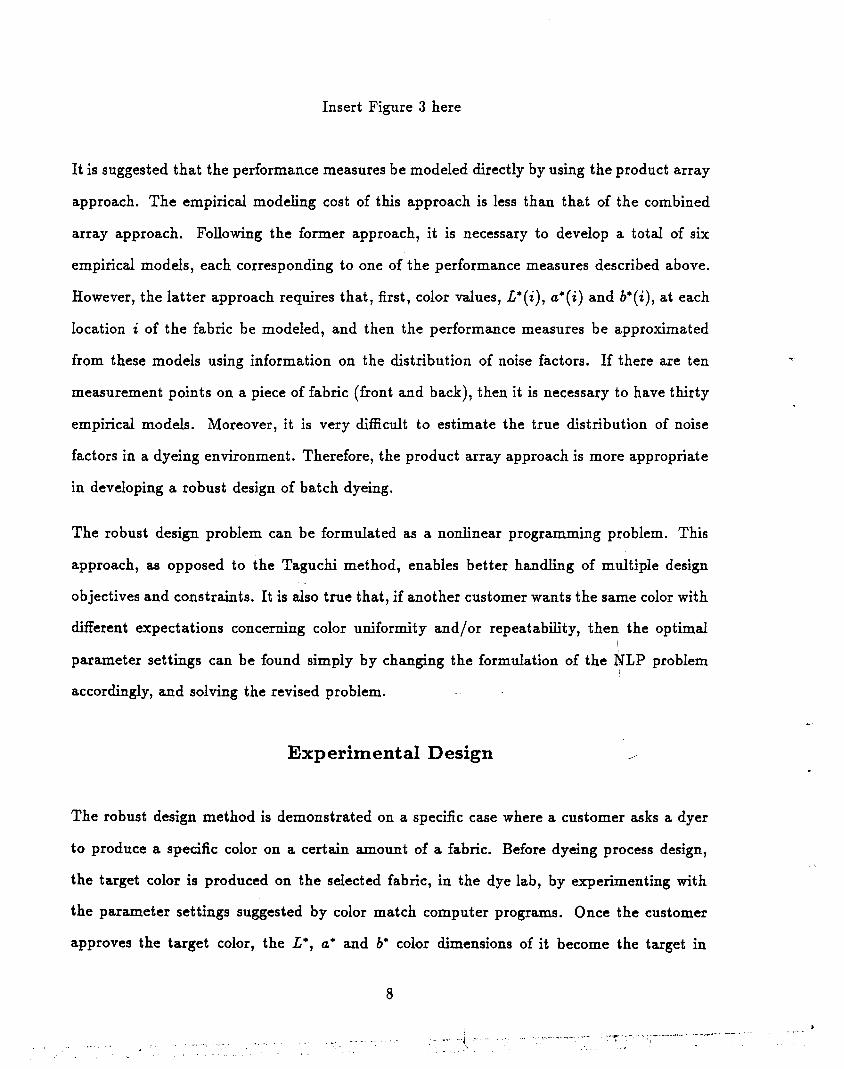
Insert Figure 3 here
It is suggested that the performance measures be modeled directly by using the product array
approach. The empirical modeling cost of this approach is less than that of the combined
array approach. Following the former approach, it is necessary to develop a total of six
empirical models, each corresponding to one of the performance measures described above.
However, the latter approach requires that, first, color values, £*(i), a*(i) and b*(i), at each
location i of the fabric be modeled, and then the performance measures be approximated
from these models using information on the distribution of noise factors. If there are ten
measurement points on a piece of fabric (front and back), then it is necessary to have thirty
empirical models. Moreover, it is very difficult to estimate the true distribution of noise
factors in a dyeing environment. Therefore, the product array approach is more appropriate
in developing a robust design of batch dyeing.
The robust design problem can be formulated as a nonlinear programming problem. This
approach, as opposed to the Taguchi method, enables better handling of multiple design
objectives and constraints. It is also true that, if another customer wants the same color with
different expectations concerning color uniformity and/or repeatability, then the optimal
parameter settings can be found simply by changing the formulation of the NLP problem
accordingly, and solving the revised problem.
Experimental Design
The robust design method is demonstrated on a specific case where a customer asks a dyer
to produce a specific color on a certain amount of a fabric. Before dyeing process design,
the target color is produced on the selected fabric, in the dye lab, by experimenting with
the parameter settings suggested by color match computer programs. Once the customer
approves the target color, the £*, a* and b* color dimensions of it become the target in
8
-.-- ..._------..- ~ ....- ..~- ..--'~''T'' '.,- ,

,.
color comparisons. Types of dyes, chemicals, fabric and equipment to be used in the process
are selected. The steps of the dyeing process are identified. These selections are shown in
Table 1. Now, it is desired to identify controllable or uncontrollable design factors, region of
experimentation and test levels of these factors.
Insert Table 1 here
Dyeing is a complex process influenced by several factors (see Koksal et al. (1990,1992)). For
the case problem, the most important factors which are controllable by the design engineer
(control factors) are identified by consulting with experts and using earlier work (see Sumner
(1976), Koksal and Smith (1991)). They are listed in Table 2 as (liquor) ratio L of volume
of dye solution (dyebath) to weight of fabric, amount of dye (based on weight of fabric) D,
salt concentration S, alkali concentration A, dyeing temperature T, time before alkali add
M, and agitation rate G (measured by twister movements per minute).
Insert Table 2 here
Many factors affecting the dyeing outcome are difficult, \expensive or impossible to controli
precisely. These include variations in the amount of dye, volume of dyebath, amount of
fabric, and characteristics of dyes, chemicals and water. The most important of these noise
factors are identified as variation in weight of dye, Wd; variation in volume of dyebath, W,,;
and variation in weight of fabric, Wi (see Table 3). Desired levels of these factors can be
simulated in a controlled dye lab environment.
Insert Table 3 here
The experiments are to be performed in a dye laboratory using a dyeing apparatus which
simulates the dyehouse dyeing. This apparatus contains glass tubes in which dyebath and
9
-.. ~.,...-- --, ..-.

a small piece of fabric is placed spiral wound around a twister (see Figure 4). Agitation
is provided by the movements of the twister. At each experiment with certain settings of
control and noise factors, a fabric piece of size approximately 6.5" x8.5" is to be dyed.
Insert Figure 4 here
The L.., a* and b* color measurements are to be made (after dyeing) at each corner and in
the middle of the fabric piece, front and back. For the particular fabric of the study case,
front and back measurements are not treated separately since there is no texture difference
between the front and the back.
As a result, ten sets of L*, a* and b* values are obtained for each experimental run i under
each setting t of the control factors (see Figure 5). These values can be summarized into two
statistics; one measuring the degree of color match, }ti, and the other showing the degree of
color uniformity, Zti, as explained before, respectively. If N pieces are sampled from those
dyed under the same setting t of the control factors, then C(N : 2) values are obtained
for the color repeatability measure Pt. Furthermore, for each control setting t, the mean of
the measures Yt, Zt and Pt are estimated as the sample mean Y t, Zt and Ph respectively,
and similarly the variances of them are estimated as the sample variances s}c' s~c and s~c'
respectively. It is also possible to combine P t and s~c into P?, to estimate the associated
quality loss due to poor color pattern repeatability. (see Figure 5)
Insert Figure 5 here
The region of experimentation is determined in such a way that the center of the region
is located close to the design point (i.e. set of process parameter settings) for producing
the color standard. Note that this design point is not necessarily robust to manufacturing
variations. The ranges of control factor settings to be tested are found based on expert
knowledge and practical limitations of laboratory testing.
10
-.."- ~.- .-"_.- ,.'-- ~
r. .' ~~ . ~.~ .
The noise factors fVd , Wv and Wf are assumed to have symmetrical distributions with mean
oand standard deviations 6%, 8% and 2%, respectively, based on earlier studies of variation
(see Sumner (1976)).
The experiments necessary for this work are chosen to be performed according to a set-up
consisting of two parts as explained before: Control factors are varied according to a design
(control array or inner array), and for each row of this design, the noise factors are varied
according to another design (noise array or outer array).
Before designing the control array, it is important to postulate a model for the performance
measures. It is assumed that the relationships between the control factors L, D, S, A, T, M, G
and the performance measures E(Yt), V(Yt), E(Zt), V(Zt) and E(pn can be approximated
by second-order polynomials.
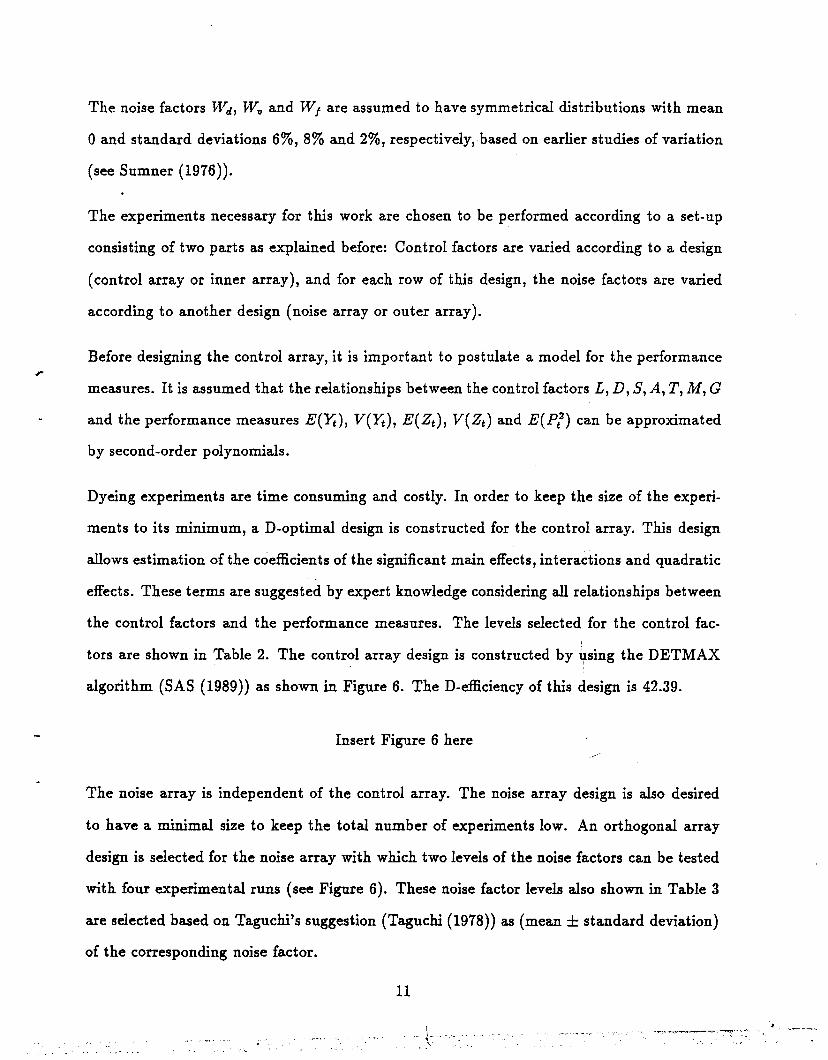
Dyeing experiments are time consuming and costly. In order to keep the size of the experi
ments to its minimum, a D-optimal design is constructed for the control array. This design
allows estimation of the coefficients of the significant main effects, interactions and quadratic
effects. These terms are suggested by expert knowledge considering all relationships between
the control factors and the performance measures. The levels selected for the control fac-i
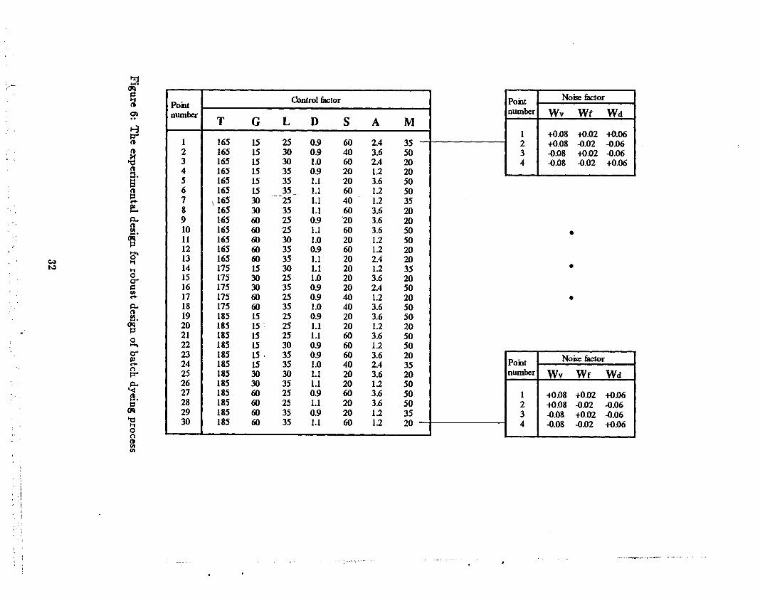
tors are shown in Table 2. The control array design is constructed by using the DETMAX
algorithm (SAS (1989)) as shown in Figure 6. The D-efficiency of this design is 42.39.
Insert Figure 6 here
The noise array is independent of the control array. The noise array design is also desired
to have a minimal size to keep the total number of experiments low. An orthogonal array
design is selected for the noise array with which two levels of the noise factors can be tested
with four experimental runs (see Figure 6). These noise factor levels also shown in Table 3
are selected based on Taguchi's suggestion (Taguchi (1978)) as (mean ± standard deviation)
of the corresponding noise factor.
11
I~-
"
The experiments are to be conducted in a well-controlled dye laboratory environment. In
experimentation, it is important to create exactly the same levels of control and noise factors
as are directed by the design, and not to introduce any other variation to the process. This
makes it possible to approximate closely the real relationships between the control factors
and the performance measures.
Conduct of Experiments
The experiments and color measurements for the particular case problem were performed, but
not in all respects as planned. The major problems encountered can be listed as inconsistent
color measurement practices and fabric installation procedure, and the use of commercial
quality dyestuff (varying dye strength). These inconsistencies were reduced significantly by
updating the data through statistical analysis, and the effects of the use of commercial quality
dyestuff use were considered negligible. Due to a misunderstanding, the laboratory technician
performed a total of sixty more experiments at additional noise settings (Wv , Wj, Wd) =
(+0.08, +0.02, -0.06) and (-0.08, -+0.02, +0.06).
The color data obtained (in terms of L*, a*, b*) for the aforementioned ten points on each
dyed fabric were first converted into performance data Yti' Zti, and Ptij, and then the perfor
mance statistics Ye, Z e, S}" S~t' and p t2 were calculated. The values obtained for the perfor
mance statistics are shown in Table 4. Also shown in Table 4 are Y t and Z t values obtained
at the process parameter settings t = (T,G,L,D,S,A,M) = (175,30,30,1.0,40,2.4,35) of
the color standard (C.S.) under a null noise array (Wv , Wf, Wd ) = (0,0,0). These values
were used in developing empirical models of the performance measures E(Yt) and E(Zt),
respectively.
Insert Table 4 here
12
••••• 0.

,.
Empirical Modeling
Performance data were analyzed and empirical models of the performance measures were
developed using the method of least squares. First, a model was selected through stepwise
regression, and weighted least squares method was utilized to estimate model parameters.
Then, the residuals obtained from the selected fitted model were checked for validity of the
assumptions of constant variance, normal error distribution, and independent errors. If the
residuals were not distributed as assumed, then the performance data were transformed to
an appropriate metric, and the same model building procedure was applied to the trans-
formed data. If the residuals of the resulting model still violated the assumptions, then the
transformed data were assigned appropriate weights and modeled again. These weights were
based on a model of the sample variances of the data.
In model selection, polynomials of order four and less were considered. Since the improve
ment in higher order polynomial fits was insignificant, second order fits were selected. Model
selection was redone after data transformation and weighting.
Applying this modeling procedure to the color match data, Yt, t = 1,··· ,31, the following
model was obtained:
log Y = -3.769891 + 0.717084S + 0.838628D + 0.757508D2 +0.006908M + 0.969541M2 + 0.017368L + 1.478919L2
0.774098T - 0.433297T2 + 1.274380LT -
0.4619I4G + 2.580223G2 + 0.753274AT +1.0I859ILM -1.69807DM + 0.437178DA
0.118293A + 1.2834I6A2 + 0.898292TM -
0.6804I5AG - 0.576239LG - 0.285780LD
0.455110LA + 0.256722GM - 0.I6I762DS +0.115107DT - 0.099368SG (1)
In this model and the others, the parameters L, D, S, A, T, M, G denote coded levels having
maximum and minimum values of +1 and -1, respectively. Table 5 summarizes the corre
sponding analysis of variance. A Box-Cox power transformation was applied to the color
13

match data, since the residuals of the best ordinary least squares (OLS) fit obtained did
not have a constant variance and normal distribution. The best power transformation was
found to be the log transformation. The OLS fit obtained for the transformed data is better
in satisfying the error distribution assumptions, but still the residuals do not appear to be
constant when plotted against the model predictions. Therefore, the above model was fitted
to the transformed data through weighted least squares (WLS). The data weights are the
reciprocal of the predicted variance of the transformed data from an OLS fit of the sample
variances. The residuals of this WLS fit validate the error assumptions (see Koksal (1992)),
and the resulting F value (156.607) and R 2 (0.9644) are satisfactory in terms of adequacy
of the fit. It should be observed from Equation (1) that the model contains many variables.
One decision criterion in model selection is to include as many significant terms as possible
in the model, and yet have enough degrees of freedom for the error. This is important to
increase prediction accuracy of the models in spite of decreased model simplicity, since these
models are to be directly used in optimization.
Insert Table 5 here
The model for color uniformity data, Zt, t - 1,···,31, was also obtained after a data
transformation and by WLS:
Z' = -4.350548 -1.433603 + 0.7813645 + 0.022431A + 0.777442AG
0.623818£S + 0.155238SA + 1.600393A2-
1.273225S2- 0.663185M - 0.298451£ +
0.549965£2 - 0.520520DM - 0.213697ST -
0.057746G - 0.345117GT - 0.831621SM +0.354170AT + 0.288962DS + 0.856133G2
-
0.276246AM - 0.186437GM + 0.096044D. (2)
The residual plots obtained from an OLS fit to the Zt data indicate that the error assumptions
are violated, and the corresponding F value (0.624) is not significant and the R2 (0.10)
is very small. The best Box-Cox transformation for the Zt data was obtained as Z: =
14

(Zt-O•5
- 1)/(-0.5). The OLS model obtained for the transformed data, Z:, satisfies the
error distribution assumptions. The F value (1.233) is still insignificant and the R2 (0.1885)
is still small. It also becomes apparent in this metric that the residuals are bigger for the data
collected from the first thirty one experiments. Since these experiments were done by using a
different fabric installation procedure, a blocking variable, 0, was added to the model which
was defined as -1 for the first thirty one experiments, and as 1 for the rest. Then, a function
was fitted to the transformed data by WLS. The weights are again reciprocals of the predicted
variances. The analysis of variance table of this fit is shown in Table 6. Residuals satisfy
error distribution assumptions (see Koksal (1992)), and the F value (11.197) is significant
and R2 (0.60) is high. Therefore, the resulting Equation (2) was selected for the mean
transformed color uniformity measure, Z'. In optimization modeling, this model is to be
used with 0 = -1, since the first thirty one experiments did not follow the correct fabric
installation procedure.
Insert Table 6 here
The function fitted for the relationship between the variance of the color match measure,
V(Y), and the control factors is:
log V(Y) - 4.447461 + 1.1668418 - 0.455444T +0.863284£8 +0.075294D - 0.145547DM - 0.227304£ - 0.097189£G +0.260337G + 0.081441A - 1.434977A 2 +0.351088T +0.108133D8 - 0.730415£2 -
0.106989£T + 0.818556D2- 0.80276782 -
0.401522£A + 0.3408728A - 0.219010G2 +0.179061M + 0.160714DA - 0.272873T2 +0.108428M2 + 0.031408DG - 0.016248G (3)
.•
This model was obtained by applying OLS directly to the logged sample variances s}.,
t = 1, ... ,30, since the log transformation stabilizes the variance of chi-squared distributed
15
I...-1.'
data such as sample variances (see Box and Draper (1987)). The residual plots indicate that
the model assumptions are satisfied (see Koksal (1992)). The F value (2020.974) is highly
significant, and R2 (0.9999) is high with 4 degrees of freedom for error. The corresponding
analysis of variance is shown in Table 7.
Insert Table 7 here
Similarly, the following model was obtained for the variance of the color uniformity measure,
V(Z):
log V(Z) - -0.585206 + 0.73295S + 0.910038T - 1.24336T2
1.126104L + 0.838461LG + 1.835292GT +1.959101SA + 1.445285LS - 0.411525A
1.450737A 2- 0.879793LD - 0.003636M
1.176581GM +0.680189AG + 0.89319M2
0.196459DT - 0.050295D - 0.893826D 2 +0.31491LA + 0.309476DS - 0.344704SG +0.513599DG - 0.579606LT + O.315453LM +0.455484L 2
- 0.211122TM (4)
The corresponding analysis of variance is summarized in Table 8. The F value (199.383)
is highly significant, and the R2 (0.9994) is high with 3 degrees of freedom for error. The
residuals also are distributed according to the model aSsumptions (see Koksal (1992)).
Insert Table 8 here
The functional relationship between the expected value of P squared, E(P 2), and the control
fac~ors was estimated by fitting a function to the P? data, t = 1,·.· ,30. The log transfor
mation was also found to be necessary for the p t2 data. The OLS fit to the transformed data
is:
16
j ..•..." ... _-
.~ .
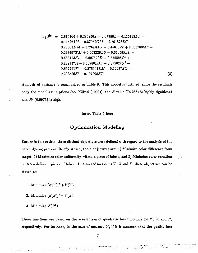
log p2 _ 2.816164 + 0.286856S - 0.07956L - 0.115732LT +0.1l5264M - 0.57959GM - 0.791528LG -
0.73301DM + 0.294041G - 0.456152T + 0.066769GT +0.287497TM + 0.603226LS - 0.510595LD +0.633413SA +0.007322D - 0.876895D2 +0.189137A - 0.302681DS + 0.375822G2
-
0.56221lT2- 0.275001LM - 0.12937SG +
0.303526S2- 0.107998ST. (5)
Analysis of variance is summarized in Table 9. This model is justified, since the residuals
obey the model assumptions (see Koksal (1992)), the F value (76.286) is highly significant
and R2 (0.9973) is high.
Insert Table 9 here
Optimization Modeling
Earlier in this article, three distinct objectives were defined with regard to the analysis of the
batch dyeing process. Briefly stated, these objectives are: 1) Minimize color difference from
target, 2) Maximize color uniformity within a piece of fabric, and 3) Minimize color variation
between .different pieces of fabric. In terms of measures Y, Z and P, these objectives can be
stated as:
1. Minimize [E(y)]2 + V(Y)
2. Minimize [E(Z)]2 + V(Z)
3. Minimize E(P2)
These functions are based on the assumption of quadratic loss functions for Y, Z, and P,
respectively. For instance, in the case of measure Y, if it is assumed that the quality loss
17
_. ,~_.oj _, _- \

increases quadratically as Y increases from zero (notice that the ideal value for Y is zero),
then it follows that the term kd(E(y»2 + V(Y)] is the expected loss due to poor color
match. In this context, k1 is the amount of quality loss at Y = 1. Similar interpretations
apply to color uniformity, measured by Z, and color repeatability, measured by P.
Other formulations of these objectives are possible. One such formulation is discussed in
Koksal (1992).
The empirical models of the previous section (or appropriate transformations of these models)
can be used to carry out the analysis.
Several approaches are typically used in modeling multiple objective optimization problems.
These include goal programming, priority ordering, and the weighted average approach,
among others. Here, the weighted average approach is described, and the reader is referred
to Koksal (1992) for a discussion of the other two approaches.
The weighted average approach is based on the following model:
Minimize
subject to -1:5 L,D,S,A,G,T,M:5 1 (6)
where kl, k 2 , ka are the corresponding weights.
We analyzed Model (6) with several sets of values for k1 , k 2 and ka• Based on the results of
our analysis, we recommend k1 = k 2 = ka = 1. The corresponding optimal solution of Model
(6) is shown in Table 10. This solution was obtained by using the NLP software EXPLORE
(see Gottfried and Becker (1973) with fifty randomly selected starting points.
Insert Table 10 here
In order to evaluate the quality level achieved at this solution, two additional sets of measures
were defined. The first set is an interpretation of the performance measures E(Y), E( Z),
18
:1.\
"'~~ t
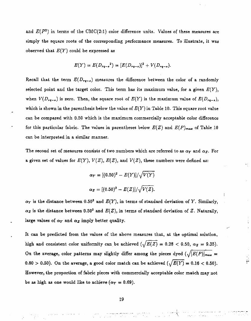
and E(P2) in terms of the CMC(2:1) color difference units. Values of these measures are
simply the square roots of the corresponding performance measures. To illustrate, it was
observed that E(Y) could be expressed as
Recall that the term E(Drq-.) measures the difference between the color of a randomly
selected point and the target color. This term has its maximum value, for a given E(Y),
when V(Drq_.) is zero. Then, the square root of E(Y) is the maximum value of E(Drq_.),
which is shown in the parenthesis below the value of E(Y) in Table 10. This square root value
can be compared with 0.50 which is the maximum commercially acceptable color difference
for this particular fabric. The values in parentheses below E(Z) and E(P)ma.a: of Table 10
can be interpreted in a similar manner.
The second set of measures consists of two numbers which are referred to as ay and az. For
a given set of values for E(Y), V(Z), E(Z), and V(Z), these numbers were defined as:
ay = [(0.50)2 - E(Y)]f JV(Y)
az = [(0.50)2 - E(Z)]f JV(Z).
ay is the distance between 0.502 and E(Y), in terms of standard deviation of Y. Similarly,
az is the distance between 0.502 and E(Z), in terms of standard deviation of Z. Naturally,
large values of ay and az imply better quality.
It can be predicted from the values of the above measures that, at the optimal solution,
high and consistent color uniformity can be achieved (JE(Z) = 0.28 < 0.50, az = 9.35).
On the average, color patterns may slightly differ among the pieces dyed (J[E(P)]ma.a: =
0.80 > 0.50). On the average, a good color match can be achieved (JE(Y) = 0.16 < 0.50).
However, the proportion of fabric pieces with commercially acceptable color match may not
be as high as one would like to achieve (ay = 0.69).
19
'.t'
Confirmation of Results
The process parameter settings found optimal as explained above were tested in the labo-
ratory under the noise array of previous experimentation to confirm the predicted results.
Laboratory performance of these parameter settings was determined by estimating E(Y),
E(Z), V(Z), V(Z) and E(P2) from the data collected. These estimates are shown in Table 11
together with the model predictions and 95 % confidence limits on these predictions.
Insert Table 11 here
Comparison of the experimental results with the model predictions shows that the tested
parameter settings yield values close to predicted values of the color uniformity measures,
E(Z) and V(Z). The value estimated from the laboratory experiments for the loss due to
poor color pattern repeatability, E(P2), is significantly less than the corresponding model
prediction and the lower 95 % confidence limit. However, the values obtained from the
experimental results for the color match measures, E(Y) and V(Y), turn out to be larger than
the upper 95 % confidence limits of the prediction. This implies that at the recommended
process parameter settings, uniform and repeatable fabric pieces can be dyed, but the color
produced may not be acceptable.
Discussion
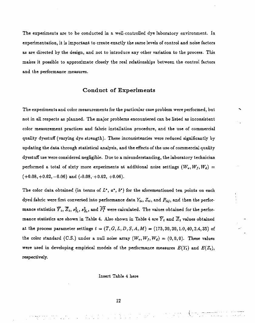
The experimental results do not confirm the predicted performance at the recommended
parameter settings with respect to the values of E(Y), V(Y) and E(P2). In this case,
the proposed design strategy (see Figure 3) requires that the sources of discrepancies be
investigated, and that the process design be fine tuned by repeating the steps of the robust
design method according to this feedback.
20
--., ._._~_._v.··_. :~-j-----;
") ' .

An analysis of the possible sources of discrepancies for the case problem is shown in Figure 7.
These discrepancies might result from design of experiments, data collection process, and/or
empirical modeling. It is our belief that the most likely causes are related to the data
collection process including experimental and measurement errors (such as use of commercial
dyestuff, and measurements on unconditioned fabric).
Insert Figure 7 here
The optimization modeling process is also revisited to investigate if another locally optimal
solution obtained could actually perform better. As mentioned before, different optimization
models of the robust design problem were developed. A number of solutions obtained from
these models were very similar. The recommended solution was only slightly better than
the others in terms of the performance measure values. One such similar solution worths
mentioning. This solution was obtained from a goal programming formulation:
Minimize
subject to
[E(y)]2 + V(Y)
[E(Z)]2 + V(Z) $ 0.25
E(p2) $ 1.00
-1 $ L,D,S,A,G,T,M $ 1 (7)
This model is aimed at obtaining the best color match with the values of [E(Z)]2 + V(Z)
and E(P2) restricted to relatively large upper bounds. The solution obtained from Model
(7) had a higher amount of dye D value (0.97), and a higher agitation rate G value (35) than
the recommended solution. At these parameter values, the models predicted that JE(Y) =0.23, V(Y) = 6.505 X 10⁻² , JE(Z) = 0.29, V(Z) = 6.270 X 10⁻⁴ and JE(P)m4t1l = 1.07.
This solution was not selected as the optimal solution, since the predicted maximum color
difference between a pair of fabric pieces was high. Now, as a result of the confirmation
21
I
:t~·_-~-"-~·-

experiments, we suspect that the color pattern repeatability model (5) overestimates its
actual value. As such, we believe that the Model (7) solution might indeed be better than
the recommended solution. This belief is also confirmed by experts in the field based on
the argument that the amount of dye suggested by the Model (7) solution is much closer to
the amount of dye used in producing the target color than the corresponding value of the
recommended solution.
The possibility that the Model (7) solution could produce better results does not answer the
question why prediction accuracy of the color match and repeatability models was poor at
the recommended solution. Therefore, to fine tune the results obtained here, we suggest that
a second set of experiments be designed and constructed to collect more data around the
recommended parameter settings, and that the empirical models and the optimal solution
be updated accordingly.
Conclusion
In batch dyeing, the main objective is to produce the target color with the least color variation
within and among dyed fabric pieces. The method provided in this paper satisfies the need
for a systematic way of finding batch dyeing process parameter settings which minimize
sensitivity of dyeing performance to manufacturing variations..
Objective quantitative evaluation of dyeing performance is made possible by the measures
developed in this work.
Design of experiments and empirical modeling of the performance measures are discussed
and demonstrated for the study case.
Formulation and solution of the robust design problem as a nonlinear programming problem
enables better handling of the multiple objectives involved. The formulation presented for
the study case is based on quality losses.
22

Confirmation of predicted results requires adequate modeling of the relationships between
the performance measures and control factors. Therefore, it is important to prevent de
viations from the designed experiment and experimental guidelines. The study case is an
example of unconfirmed results at the first iteration of the method due to deviations from
the experimental guidelines. It is suggested that a second iteration be performed to design
additional experiments and collect more data to update the empirical models.
The proposed design approach can also be used to design other chemical batch processes such
as industrial painting or plating. It is especially recommended for problems with many design
objectives. For each case, of course, it is necessary to formulate appropriate performance
measures.
23

Acknowledgements
The authors gratefully acknowledge the support of the Consortium for Research in Apparel,
Fiber and Textiles Manufacturing (CRAFTM) and the National Textile Center (NTC) for
funding this work. We also thank Ciba-Geigy Dyestuff and Chemicals Division in Greens
boro, North Carolina for the assistance and facilities they provided for the experiments and
measurements involved in this work.
24
References
AATCC. (1989) "CMC: Calculation of Small Color Differences for Acceptability," Teztile
Chemist and Colorist 21, 11, pp. 18-21.
Box, G.E.P., and Draper, N.R. (1987). Empirical Model-Building and Response Surfaces,
New York, John Wiley & Sons.
Fathi,Y. (1991). "A Nonlinear Programming Approach to the Parameter Design Problem,"
European Journal of Operational Research 53, 3, pp.371-381.
Gottfried, B.S. and Becker, J.R. (1973). EXPLORE: A Computer Code for Solving Nonlinear
Continuous Optimization Problems, Technical report no. 73-6, Department of Operations
Research, University of Michigan.
Koksal, G., and Smith, W.A.,Jr. (1990). System Analysis for Dyehouse Quality Control,
Technical report no. 90-3, Dept. of IE, NCSU, Raleigh, NC 27695.
Koksal, G., and Smith, W.A.,Jr~ (1991). Quality Function Deployment: A Multi-stage
Application Perspective and a Case Study, Technical report no. 91-6, Dept. of IE, NCSU,
Raleigh, NC 27695.
Koksal, G., Smith, W.A.,Jr., and Smith, C.B. (1992). "A -'System' Analysis of Textile
Operations - A Modem Approach For Meeting Customer Requirements," Teztile Chemist
and Colorist 24, pp. 30-35.
Koksal (1992). Robust Design of Batch Dyeing Process, Ph.D. dissertation, Dept. of IE,
North Carolina State University, Raleigh, NC 27695.
Leon, R.V.; Shoemaker, A.C, and Kacker, R.N. (1987). "Performance Measures Independent
of Adjustment, An Explanation and Extension of Taguchi's Signal-to-Noise Ratios" (with
discussion), Technometrics 29, 3, pp.253-285.
25
.. .-._~--~.---~.-
Mesenbrink, P., Lu, J.C., McKenzie, R., and Taheri, J. (1992), "Characterization and Op-
timization of a Wave Soldering Process", in revision for Journal of the American Statistical
Association.
Phadke, M.S. (1989). Quality Engineering Using Robust Design, Prentice-Hall.
SAS Institute Inc. (1989). SAS/QC Software: Reference, Version 6, First Edition, Cary,
NC: SAS Institute Inc.
Shoemaker, A.C., Tsui, K.L., and Wu, C.F.J. (1989). Economical E::perimentation Methods
for Robust Parameter Design, IIQP Research Report No. RR-89-04, The Inst. for Improve
ment in Quality and Productivity, Univ. of Waterloo, Waterloo, Ontario, Canada, N2L
3G1
Sumner, H.H. (1976). "Random Errors in Dyeing - The Relative Importance of Dyehouse
Variables in the Reproduction of Dyeings," Journal of the Society of Dyers and Colourists,
pp. 84-99.
Taguchi, G. (1978). "Performance Analysis Design," International Journal of Production
Research 16, pp. 521-530.
,
Tagucbi, G. (1986). Introduction to Quality Engineering, Asian Productivity Organization.
Vining, G.G. and Myers, R.H. (1990). "Combining Taguchi and Response Surface Philoso
phies: A Dual Response Approach," Journal of Quality Technology 22, 1, pp.38-45.
Key Words: Off-Line Quality Control, Quality Engineering, Parameter Design, Robust De-
sign, Design Optimization, Te::tiles Dyeing, Color Control.
26
-.

Greige Fabric Chem.'s Water Dyes
PREPARE
DYE
FINISH
Finished Fabric
Figure 1: Dyehouse operations flowchart
27
-i--------, .

j .,
Ca*b*
Figure 2: CMC(2:1) unit acceptance volume
28
L*

.#
r----.PERFORMANCE MEASUREFORMULATION
EXPERIMENT DESIGN
EXPERIMENTATION
DATA ANALYSIS(p.M. MODELING)
NLP FORMULATION&SOLUIlON
CONFlRMATION
Figure 3: Robust design method
29
...
• __._.."-~' _..,..'_ • ~., ~. ,,":; ......"Or:Y:"::~•
<·It.- ,.. . ...~-,

.. ~ .
'" . ,- ....
GLASS BEAKER
Figure 4: Ahiba-Texomat dyeing machine/
30
.·

L* til 1 P tI2 I Yt
a* tilPt13
b* til I Zt
Yti, Zti P tIN
L* ti,lO I P t23 ~2
SYt
a* ti,IO
b* ti,lO) P t2N 2SZt
-P t,N-I,N P~
j,1Ii,
,j
-j,"I.:,1
I'%j....oq
~
"C11..S'0-l=lt/)....p..
"t/)....cap...
~III
~ S..... p...
"0
"S-asn
"!3tI
c:~tIt/)
00-....21.~
"p...
1: ~
\
COLORDATA
PERFORMANCEDATA
PERFORMANCEMEASURES
:/J>o- _0
i,j
~t-.)
I'%j
~.
~0)..~CD
~CDt:l.13CDae.p..CDIn....~8't;
t;o0'"~In....p..CDIn
e§'g,0'"~(')
P"'
~CDs·
(Jq
"dt;o(')CDInIn
Control fuctor Poilt Not;e fuctorPoilt
number Wv Wf WdnumberT G L D S A M
1 +0.08 +0.02 +0.061 165 15 25 0.9 60 2.4 35 2 +0.08 ·~)'o2 -0.062 165 15 30 0.9 40 3.6 50 3 -0.08 +0.02 -0.063 165 15 30 1.0 60 2.4 20 4 -0.08 -0.02 +0.064 165 15 35 0.9 20 1.2 205 165 15 35 1.1 20 3.6 506 165 15 3~_ 1.1 60 1.2 507 \ 165 30
.'-~
25 1.1 40 1.2 358 165 30 35 1.1 60 3.6 209 165 60 25 0.9 '20 3.6 2010 165 60 25 1.1 60 3.6 50 •11 165 60 30 1.0 20 1.2 5012 165 60 35 0.9 60 1.2 2013 165 60 35 1.1 20 2.4 2014 175 15 30 1.1 20 1.2 35 •15 175 30 25 1.0 20 3.6 2016 175 30 35 0.9 20 2.4 5017 175 60 25 0.9 40 1.2 20 •18 175 60 35 1.0 40 3.6 5019 185 15 25 0.9 20 3.6 5020 185 15 . 25 1.1 20 1.2 2021 185 15 25 1.1 60 3.6 5022 185 15 30 0.9 60 1.2 5023 185 15 ' 35 0.9 60 3.6 20 Not;e fuctor24 185 15 35 1.0 40 2.4 35 Pont25 185 30 30 1.1 20 3.6 20 number Wv Wf Wd26 185 30 35 1.1 20 1.2 5027 185 60 25 0.9 60 3.6 50 1 +0.08 +0.02 +0.0628 185 60 25 1.1 20 3.6 50 2 +0.08 -0.02 -0.0629 185 60 35 0.9 20 1.2 35 3 -0.08 +0.02 -0.0630 185 60 35 1.1 60 1.2 20 4 -0.08 -0.02 +0.06

Use of commercialdye
Improper dyestorage
,..-- Model selection
~- Model fitting
--- Performancemeasures
~-- Experimentation.. region
/-40-- Construction
Measurements onunconditionedfabric -----~
Inconsistent fabricinstaDation
ROBUST DESIGN DATACOLLECI10N
Nomefactors ~"'-f
Inconsistent colormeasurements
Figure 7: Possible sources of discrepancies
....
33

DYE
CHEMICALS
FABRIC
DYEING MACHINE
DYEING PROCEDURE
~ '-,'-",
Table 1: The case problem
Cibacron BR Red 4G-E
Irgasol CO-NF, Reserve Salt Flake, sodium chloride,
soda ash, caustic soda, Silvatol AS Cone
100% cotton left hand twill, commercially prepared
Ahiba-Texomat
Batch Exhaust Dyeing
34
".
_'~""-'------,

Table 2: Important control factors and their levels
Levels
Control Factors (-1) (0) (+1)
L: Liquor ratio [mL/g] 25 30 35
D: Amount of dye [% om] 0.9 1.0 1.1
S: Salt concentration [giL] 20 40 60
~: Alkali concentration [giL] 1.2 2.4 3.6,I
T:Dyeing temperature [OF] 165 175 185.
M: Time before alkali add [min] 20 35 50
G:..-Agitation rate [movements/min] 15 30 60
35
.- .~. -.. '.

Table 3: Important noise factors and their levels
Levels
Noise Factors (-0-) (+0-)'" ;
!
Wd : Variation in dye weight (%) -0.06 +0.06
Wv : Variation in dyebath volume (%) -0.08 +0.08!
I
WJ: Variation in fabric weight (%) -0.02 +0.02
36
...~.
...

Table 4: Performance statistics calculated from the experimental data
ControlSetting Y t
t
2SZe
1 2.479 0.279 4.049 0.168 13.5062 10.956 0.400 14.854 0.227 5.9673 16.678 0.386 80.456 0.228 92.8424 9.234 0.400 16.615 0.317 9.5535 5.371 0.343 7.086 0.271 7.6936 3.351 0.244 3.808 0.194 8.3647 4.055 0.239 6.534 0.185 11.7288 9.666 0.346 35.306 0.214 43.4939 3.337 0.317 6.436 0.368 27.526
10 2.496 0.272 0.710 0.261 2.54811 21.505 0.394 38.587 0.445 3.40212 12.918 0.317 25.804 0.331 3.56013 8.108 0.250 47.305 0.171 26.35814 14.480 0.466 62.544 0.722 24.73315 4.649 0.177 2.579 0.039 5.85916 3.254 0.059 0.879 0.000 2.21717 19.907 0.318 43.599 0.281 6.90318 2.993 0.086 1.776 0.001 2.32719 2.367 0.108 0.528 0.003 1.22720 3.652 0.202 3.076 .-0.033- 5.12221 3.378 1.069 1.450 5.680 5.64922 15.460 0.521 26.395 1.067 6.77823 14.201 0.260 29.391 0.083 15.569
/24 7.084 0.248 15.598 0.078 18.26925 5.250 0.143 9.600 0.008 11.94326 5.903 0.106 12.989 0.001 9.89027 14.913 0.201 55.755 0.012 19.72028 4.085 0.127 8.684 0.009 21.515 n'
:':i
29 10.480 0.160 39.596 0.004 22.895 "l
30 4.386 0.106 8.583 0.004 14.136C.S. 0.036 0.069
1.\
37
-. _. _._., ,n.~
~

Table 5: Analysis of variance for log Y
Source DFSum of
SquaresMean
Square F Value Prob>F
Model 27 4191.93741 155.25694 156.607 0.0001
Error 156 154.65493 0.99138
C Total 183 4346.59234
Root MSE 0.99568 R,square 0.9644I
Dep Mean 0.81132 Adj R-sq 0.9583
C.V. 122.72328
38
i
j,". \,'.
..

Table 6: Analysis of variance for Z'
Source DFSum of
SquaresMean
Square F Value Prob>F
Model 22 142.03562 6.45616 11.197 0.0001
Error 161 92.83252 0.57660
C Total 183· - 234.86814
Root MSE 0.75934 R-square 0.6047
I. -I,
,
Dep Mean -4.00201 Adj R-sq 0.5507
C.V. -18.97399
39
":-
..--.... - -... _ ..~--~-',' .: ..-.

Table 7: Analysis of variance for log s}
Source DFSum of
SquaresMean
Square F Value Prob>F
Model 25 58.01006 2.32040 2020.974 0.0001
Error 4 0.00459 0.00115
C Total 29 58.01465
Root MSE 0.03388 R-square 0.9999
Dep Mean 2.29033 Adj R-sq 0.9994
C.V. 1.47946
40
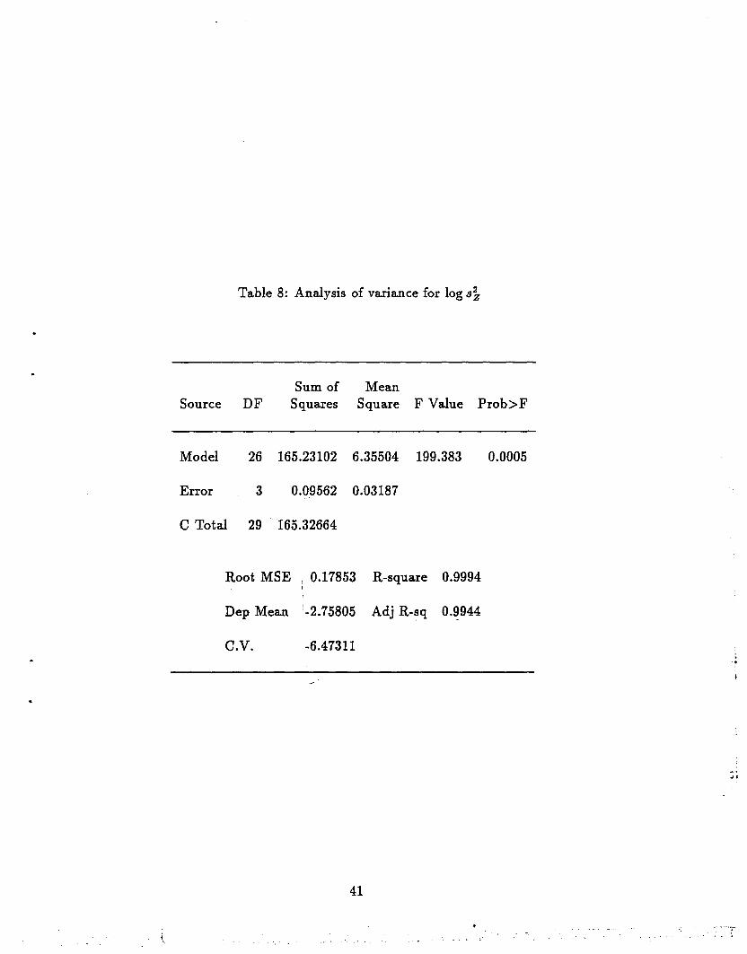
Table 8: Analysis of variance for log s~
Source DFSum of
SquaresMean
Square F Value Prob>F
Model 26 165.23102 6.35504 199.383 0.0005
Error 3 0.09562 0.03187
C Total 29165.32664
Root MSE I 0.17853 R-square 0.9994I
Dep Mean -2.75805 Adj R-sq 0.9944-
C.V. -6.47311 ,,,.
~
.,
41

Table 9: Analysis of variance for log p2
Source DFSum of
SquaresMean
Square F Value Prob>F
Model 24 26.96182 1.12341 76.286 0.0001
Error 5 0.07363 0.01473
C Total 29· - 27.03545
Root MSE 0.12135 R-square 0.9973
Dep Mean 2.26256 Adj R-sq 0.9842
C.V. 5.36348
42
!
i\
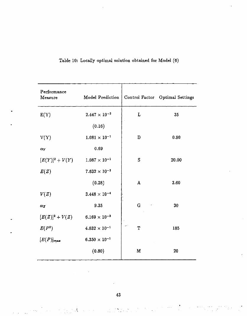
Table 10: Locally optimal solution obtained for Model (6)
PerformanceMeasure Model Prediction Control Factor Optimal Settings
E(Y) 2.447 X 10⁻² L 35
(0.16)
V(Y) 1.081 x 10⁻¹ D 0.90
ay 0.69
[E(Y)]2 + V(Y) 1.087 X 10⁻¹ S 20.00
E(Z) 7.632 X 10⁻²
(0.28) A 3.60
V(Z) 3.448 x 10⁻⁴
az 9.35 G 30
[E(Z)]2 + V(Z) 6.169 X 10⁻³
E(P2) 4.032 X 10⁻¹~-
T 185
[E(P)]~tU: 6.350 x 10⁻¹
(0.80) M 20
43
1, _,_ c
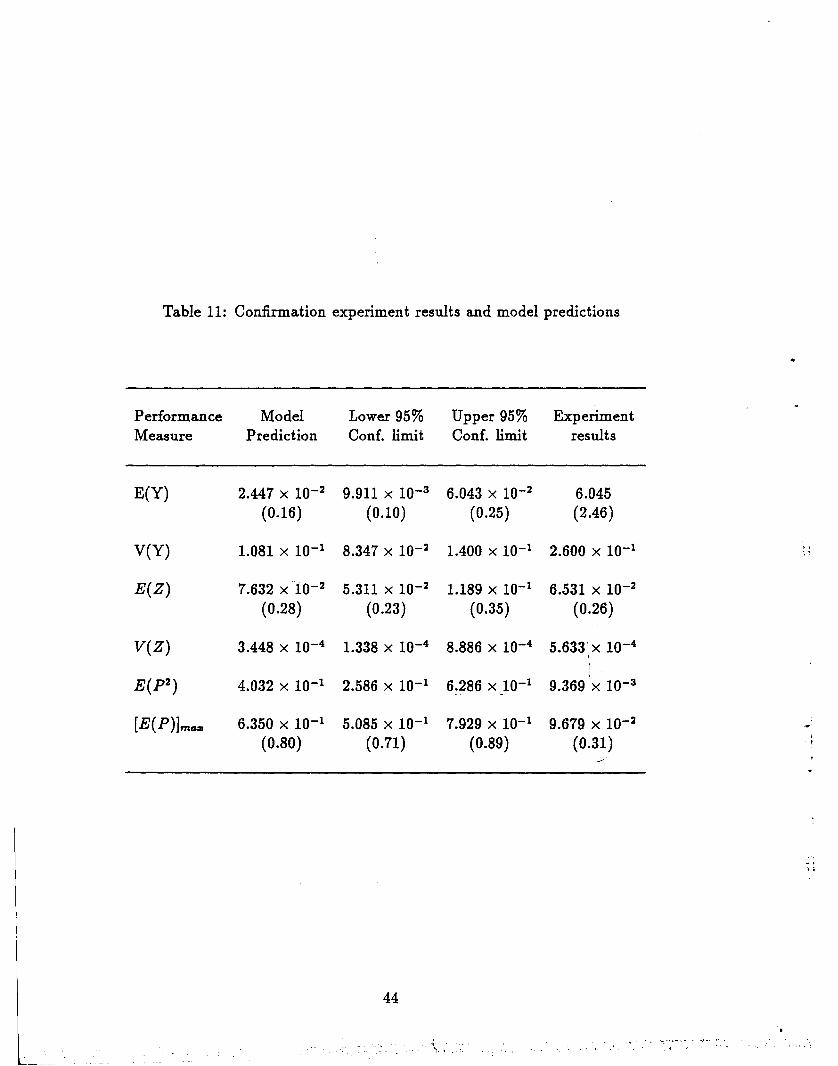
Table 11: Confirmation experiment results and model predictions
PerformanceMeasure
ModelPrediction
Lower 95%Coni. limit
44
Upper 95%Coni. limit
I
\.
Experimentresults
• '-. -, -~"'o ...... , ...... _ •. '" -.
! l
,.

YY±YYYYYYYY
WordPerfect tips and tricks: columns and tables in WP DOSand WP Windows. Monday, 19 A~ril, from 10:00 to noon in theFaculty Senate Room of D.H. H1ll Library
WordPerfect tips and tricks: mail merge in WP DOS and WPWindows. Monday, 3 May, from 10:00 to noon in the FacultySenate Room of D.H. Hill Library.
P File Edit Manage Window setup Help 10:13:12eeeeeeeeeeeeeeeeeeeeeeeeeeeeeeeee INBOX Viewer eeeeeeee [ ] Index eeeeeeeee[]e£° Thu, 15 Apr 93 13:26:15 EDT °° To: [email protected] °o 0o 0o 0
° From: <[email protected]> °° SUbject: Prompt, 15 April 1993 °° Message 3 of 11 °opresent the following:
°ooooooo
°0Flease join us for one or both of these seminars. They are open toofacuIty, staff, and students; no registration is required.
°aeeeeeeeeeeeeeeeeeeeeeeeeeeeeeeeeeeeeeeeeeeeeeeeeeeeeee±YYYYYYYYYYYYYYYYYYYYY¥F2 Compose F3 Fetch F4 Forward F5 Reply F6 Delete F7rev Msg F8Next Msg