serial correlation statistics of written texts - gelbukh.com · serial correlation statistics of...

IJCLA VOL. 3, NO. 2, JUL-DEC 2011, PP. 11–43 RECEIVED 16/09/12 ACCEPTED 18/12/12 FINAL 23/12/12

Serial Correlation Statistics of Written Texts

MARK PERAKH1

California State University Fullerton, USA

ABSTRACT

Serial correlation statistics has been widely used in various fields of science, but apparently has not yet been applied to the analysis of texts. In this paper a method is offered using measurements and computations of certain statistical sums that reflect the variability of the letters’ distribution along texts. It opened a way for the analysis of texts’ structure not available by other means and thus led to the discovery of hidden regularities in the structure of semantically meaningful texts, including, for example, an “average domain of minimal letters variability,” common for all semantically meaningful texts in various languages, but absent in meaningless strings of symbols. Another revelation was the connection of certain serial correlation parameters with Zipf’s law.

KEYWORDS: quantitative linguistics, Zipf law.

1 Introduction

Serial correlation statistics (also referred to as autocorrelation) is widely used in such diverse areas as, for example, econometry [1], spectroscopy [2], or even in music recording [3], and in many other areas. However, to the best of the author’s knowledge, it has not yet been applied to the analysis of texts. In this paper a method is described

1 Mark Perakh passed away soon after submitting this paper, his last publication. The text was copy-edited and formatted later; errors inadvertently introduced in this process are responsibility of the editor.

MARK PERAKH 12

making use of the serial correlation, which in this case will be dubbed Letter Serial Correlation (LSC). It turned out to be a rather powerful tool leading to the discovery of hitherto unknown features of the texts’s intrinsic structure.

It is reasonable to assume that meaningful texts possess a certain degree of order. The entropy of meaningful texts is expected to be somewhere between the low entropy of highly ordered meaningless strings and the high entropy of chaotic meaningless strings.

Entropy, though, characterizes the overall level of the disorder in a text but does not reveal the specific features of a text’s structure. Therefore it is desirable to develop methods for analyzing specific forms of order in texts.

Imagine that we try to decipher a text written in an unknown language. First we have to determine whether the string of symbols in question is a meaningful text or is gibberish. Information theory is not helpful in this case because its tools are indifferent to the semantic contents of the text. The method of strings’ analysis developed in the Algorithmic Probability/Complexity theory [4, 5, 6], while adding a powerful tool to the arsenal of mathematics, linguistics, biology and other fields of inquiry, leaves out the problem of distinguishing between meaningful texts and gibberish. Recent developments in this area [7], while introducing certain markers of noise vs. meaningful messages, do not seem suited to deciphering texts in unknown languages.

In this paper a method for unearthing certain specific structural properties of texts is suggested. It has revealed hidden regularities in meaningful texts’ structures. These regularities happen to be present in a wide variety of languages that use alphabetical systems of writing. This method uses a statistical approach based on the analysis of the variability of symbols’ distribution along the string. It will be referred to as the Letter Serial Correlation statistics, or simply LSC.

2 Basics of the LSC Method

Imagine a string N symbols long. The symbols can be, for example, letters drawn from an alphabet that comprises Z different letters. It can be a text in English, say the Song of Hiawatha by Longfellow, wherein N = 141,399 and Z = 26; it can be the German text of any of Goethe’s novels where Z = 26 and N varies from novel to novel. It can be the

SERIAL CORRELATION STATISTICS OF WRITTEN TEXTS

13

Hebrew text of the Book of Genesis, which is N = 78,064 letters long, with Z = 22. It can be a computer program written as a string of zeros and ones, so Z = 2. It can even be a biological macromolecule wherein each “letter” is a specific chemical compound, etc.

There are three versions of the LSC method. However, of the three versions one turned out to be most informative, therefore in this paper only the data obtained by that version are reported.

When we say that the text’s length is found to be N letters long, this number excludes spaces between the words and punctuation marks. We divide the text into equal cells, each n letters long. If N is divisible by n, then the number k of cells will be k = N / n. If, though, N is not divisible by n, then the last cell at the end of the text will be shorter than the rest of the cells. If k is the number of the “full” cells, each of the same size n, then the total number of cells, including the partial cell at the text’s end, will be r = k +1. In such cases the last, partial cell will be cast off and not accounted for.

Let us denote the length of the truncated text, that is the length remaining after casting off the partial end cell, expressed in the number of letters, as L. Obviously, if N is divisible by n, L = N, and k = r, otherwise L = kn < N.

Let us count how many times each letter of the alphabet appears in the entire text, and denote these numbers as Mi ,where the index i takes the values between I = 1 (for the first letter of the alphabet) and I = Z (for the alphabet’s last letter).

Let us assign to the cells, remaining in the text after truncation (if such was necessary) numbers from j = 1 (starting at the text’s beginning) to j = k.

Denote by Xi,j the number of occurrences of letter xi in the cell number j and by Xi,j+1 the number of occurrences of the same letter xi in the neighboring cell number j+1 . Consider the expression (Xi,j – Xi,j+1)2. Squaring the difference ensures the independence of the calculated quantity on whether the letter xi occurs more often in cell j or in cell j + 1.

Comment. Obviously, each cell contains a n-gram. Therefore, some readers may get the impression that we deal here with n-gram statistics. In fact, the serial correlation statistics is quite different from a n-gram statistics. A couple of simple examples may help to see this difference. Let us choose n = 3. Then each cell contains a trigram. Consider a pair of neighboring cells, one containg the trigram [abc] and the other the trigram [def]. What if we shuffle the letters in the cells, getting now a

MARK PERAKH 14

pair of cells containing, one the trigram [acb] and the neighboring cell containing the trigram [efd]? From the viewpoint of the trigram statistics, the trigrams [abc] and [acb], as well as [def] and [efd], are different trigrams and should be treated as such as long as the trigram statistics is applied. On the other hand, within the serial correlation statistics there is no difference between the cells containing either trigram [abc] or trigram [acb]. Indeed, the expression (Xi,j – Xi,j+1)

2, which is at the core of the letter correlation statistics, does not depend on the order of letters within the cells. Letter correlation statistics is concerned with the variability of letters along the string and is indifferent to the fact that cells contain n-grams.

Another example of the difference between the approaches of the n-gram and the serial correlation statistics is as follows: the n-gram statistic is only interested in such n-grams which can happen in the explored texts. For example, the trigram [zth] normally does not happen in English texts and therefore it is of no interest for n-gram statistics. Imagine, though, the following string is found in some text: “The word ‘heart’ in German is ‘Herz’. This translation can be found in a dictionary.” Choose n = 3. Then it can happen that one of the cells will contain the following combination of symbols: [z’.(space)Th]. From the viewpoint of the serial correlation, where spaces and punctuation marks are ignored, this combination is equivalent to a cell containing the trigram [zth], and is a legitimate element of the serial correlation statistics.

Now define the following sum, which is referred to as the Measured Letter Serial Correlation (LSC) sum:

( )∑∑=

−

=+−=

Z

i

k

jjijim XXS

1

1

11,, . (1)

The first summation in equation (1) is performed over all letters of the available alphabet, from I = 1 to I = Z. The second summation is over all pairs of neighboring cells, numbered from j = 1 to j = k – 1. (Each cell, except for cells number 1 and number k, appears twice in the equation, once paired with the preceding cell and once paired with the subsequent cell; the number of boundaries between the cells, which also is the number of pairs of neighboring cells, is k – 1).

If measured on a specific text and calculated by equation (1), the sum Sm statistically estimates the variability of letter distribution along the text, averaged over its length.


15

The interpretation of the behavior of Sm can be facilitated if it is compared with the Expected Letter Serial Correlation sum, to be denoted Se. For a randomized text Se can be calculated exactly. When calculating the expected letter serial correlation sum, a perfectly random text must be distinguished from the texts obtained by permutations of letters of a meaningful text. In a perfectly random text each letter of the available alphabet has the same probability of appearing at any location in the text. On the other hand, in a text obtained by a permutation of a meaningful text, the frequency distribution of letters is the same as in the original text (the latter to be also referred to as the identity permutation). Therefore in the permuted texts the probabilities of appearing at a certain location in the text are different for each letter.

For example, in English, German, and Spanish texts the most frequent letter is e (which in sufficiently long English texts usually occupies about 12 percent of the text). Hence, in a gibberish text obtained by permutation of, say, a sufficiently long English text, the letter e will also appear at approximately 12 percent of the locations, so the probability of that letter appearing at an arbitrary location is about 0.12. For the least frequent letter, z, the probability in question is only a fraction of one percent. On the other hand, in a perfectly random text, using the same 26 letter-long alphabet, the probability in question for both e and z is the same, about 1 / 26.

If a certain letter appears M times in the identity permutation, it will also appear M times in any permuted version of the text in question. On the other hand, this letter, as well as any other letter of the alphabet in use, will appear close to N / Z times in a perfectly random text of the same length of N letters.

In view of the above, the calculation of the expected letter serial correlation sum must be conducted differently for the texts obtained by permutations of a meaningful text and for perfectly random texts. However, the pertinent calculation has revealed that the formulae for Se, derived for texts randomized by permutation and for a perfectly random text, differ only by the factor L / L – 1, where L is the total number of letters in the text (truncated when necessary as described above). Since the studied texts comprised at least several thousand letters each, the above factor was practically equal to 1, so the quantitative difference between expected LSC sums calculated for texts randomized by permutations of letters of a meaningful texts and the sums for perfectly random texts turned out to be negligible.

MARK PERAKH 16

The expected letter serial correlation sum is calculated by the following equation (derived in Appendix 1):

∑= −

−

−=Z

i

iie L

MLM

L

nS

1 112 . (2)

The summation in equation (2) is performed over all letters of the alphabet in use.

For the texts subjected to the study, both the measured letter serial correlation sum (as per equation 1) and the expected letter serial correlation sum (calculated by equation 2) are determined for a series of values of the cell size n. This results in two sets of data, one representing the functional dependence of Sm on n, and the other of Se on n.

These data carry information about the text’s structure insofar as it is reflected in the variability of letters distribution along the text.

In many cases it turns out useful to study letter serial correlation utilizing, besides LSC sums, also certain auxiliary quantities. One such quantity is what will be called Letter Serial Correlation density. This quantity is obtained by dividing the LSC sums by the cell size n. We distinguish between the measured LSC density dm, and expected LSC density de. For example, the expected LSC density is calculated as

∑= −

−

−=Z

i

iie L

MLM

Lnd

1 1

112 . (3)

Since LSC densities are obtained from the data on LSC sums, they can’t provide information beyond that inherent in the LSC sums. However, in certain cases reviewing the data for LSC densities makes it easier to interpret the observed data. Furthermore, the use of LSC densities revealed the connection between the LSC and Zipf’s law [8], as will be shown later in this paper.

Another auxiliary quantity is what will be called specific letter serial correlation sums. This quantity is obtained through dividing the LSC sum (either the measured or the expected) by the truncated text’s length L. Since in the specific LSC sums, unlike the original LSC sums, the possible effects of the difference in the text’s lengths are eliminated, the specific sums are useful if texts of various lengths are to be compared.

Equation (2) represents, theoretically, a straight line in coordinates Se – n. At n=1 the expected LSC sum has the value of


17

∑= −

−

−=Z

i

iie L

MLM

LS

1 1

112 . (4)

and theoretically it drops to zero at n = L. In fact, though, the Se – n curve is not exactly a straight line, because the truncated length L of a text (which is part of the equation in question) is obtained by casting off the last, incomplete cell. If the total text’s length N is divisible by n, there is no incomplete cell at the text’s end, and L=N. If, though, N is not divisible by n, the last, incomplete cell, whose size may vary between 0 and n – 1, is cast off, so that the truncated text’s length L may vary, depending on the values of N and n, between L = N and L = N – (n – 1). As a result, the actual Se – n curve consists of small steps rather than being an exact straight line, as equation (2) implies. Fortunately, the steps on the Se – n curve are small (except for very large n) and do not mask the overall linear dependence of S on n, as theoretically predicted.

Let us write the theoretical equation for the expected LSC density (de = Se / n) in the following form:

n

QTdd et =+= , (5)

where de is expressed by equation (3) and the constants T and Q are as follows:

∑= −

−=

Z

i

ii L

MLM

LT

1

,1

2 (6)

∑= −

−=

Z

i

ii L

MLMQ

1

.1

2 (7)

Equation (5) represents the theoretical hyperbolic function. In logarithmic coordinates, the corresponding theoretical curve is a straight line. However, because the truncation of the text’s length, described above, varies for different values of n, the actual curve deviates from the theoretical straight line. To account for that deviation, equation (5) can be modified as follows :

,1

Tn

QTddqte −=−= (8)

where for the theoretical function the exponent q = 1, but for the actual experimental “curve” it is slightly different from q = 1.

MARK PERAKH 18

All the equations (2) through (7) have been derived for a hypothetical randomized text in which the total number N of letters as well as the numbers of appearances of each letter in the text equal these numbers in the original meaningful text. However, for the original meaningful text itself a theoretical calculation of the LSC sums, LSC densities, and specific LSC sums is impossible, because the intrinsic structure of such a text is yet unknown. These quantities have to be found experimentally.

The LSC data for meaningful texts have been obtained by applying a computer program which counted the total number N of letters in the text, as well as Mi – the numbers of occurrences of each letter in the text, divided the texts into k cells each of length n, cast off the incomplete cell if such happened to appear at the text’s end, thus truncating the text’s length to L, and finally calculated the measured LSC sum Sm, according to equation (1). This operation was repeated for a series of values of n, the cell’s size. The described operation produced a set of values of Sm as a function of n. The program had also computed, using eq. (2), the expected LSC sum, Se, for the same set of values of n.

More than 90 letter strings have been studied, including natural meaningful texts in various languages (Aramaic, Hebrew, Latin, Greek, English, Russian, German, Spanish, Italian, Czech, Finnish, and Yiddish). The LSC data displayed distinctive statistical features, qualitatively identical for all meaningful texts, regardless of language, topic, style, or authorship. These features were, however, absent in meaningless texts, either in artificially constructed, highly ordered ones, or in strings of gibberish randomized in various ways.

3 Experimental Data

The lengths of the studied texts varied from about 5,000 letters to over two million letters. The studied texts included 13 books of the Bible in Hebrew, translations of the Book of Genesis into all the listed languages except Yiddish, the entire text of the Torah (the Pentateuch) both in Hebrew and in Aramaic, the Book of Isaiah in Italian, the entire text of the Talmud (which is partly in Hebrew and partly in Aramaic), translations of a part of Tolstoy’s novel War and Peace into Hebrew and English, the entire text of Melville’s novel Moby Dick in English, the United Nation’s Sea Trade Treaty in English, Shakespeare’s


19

Macbeth in English, Longfellow’s Song of Hiawatha in English, collections of short (published) stories by the author of this article, one set in English and the other in Russian, and the full text of one issue (October 16, 1988) of the newspaper Argumenty i Fakty (“Arguments and Facts”) in Russian. Besides the listed original texts, LSC measurements were also conducted on the same texts from which either all vowels or all consonants were removed. Furthermore, experiments were conducted with various artificially constructed texts. Among these artificial texts were highly ordered texts with precisely known structures, for which the LSC sums could be exactly calculated and the results of calculations could be compared with the experimentally measured quantities, thus testing the understanding both of the outcomes of measurements and of the texts’ structure.

Also among the studied texts were strings with various degrees of randomness. Some of them were obtained by computer permutations of various elements (paragraphs, verses, words, letters, etc.) of meaningful texts. Other randomized texts were the results of a deliberate effort to artificially create random gibberish from scratch.

Finally, LSC statistics was applied to the yet undeciphered medieval text known as the Voynich manuscript, written in an unknown language and an unknown alphabet. The results of this study are not reported in this paper for two reasons. First, the scope of the obtained data was so large that it would require a separate paper of an even larger size than this one, and that material is more of a cryptological than of a linguistic interest. Secondly, while the results of the study of the Voynich manuscript by the LSC technique seemed to be of great interest, as they shed light on many hitherto unknown characteristics of the manuscript, they had not led to deciphering that mysterious text.

We can generalize the main results of our study as the following two statements:

1. The behavior of the Letter Serial Correlation sums displays certain systematic features, common for all studied texts, regardless of the language, topic, gist, authorship, or style. These features, in particular, distinguish semantically meaningful texts from meaningless strings of characters (thus usually enabling one to determine whether a text is meaningful or gibberish even if its language and/or the meanings of the alphabetical symbols are unknown).

MARK PERAKH 20

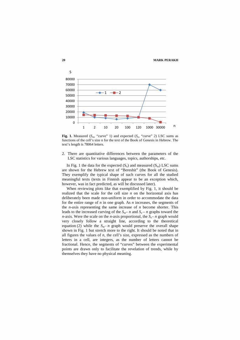
Fig. 1. Measured (Sm, “curve” 1) and expected (Se, “curve” 2) LSC sums as functions of the cell’s size n for the text of the Book of Genesis in Hebrew. The text’s length is 78064 letters.

2. There are quantitative differences between the parameters of the LSC statistics for various languages, topics, authorships, etc.

In Fig. 1 the data for the expected (Se) and measured (Sm) LSC sums are shown for the Hebrew text of “Bereshit” (the Book of Genesis). They exemplify the typical shape of such curves for all the studied meaningful texts (texts in Finnish appear to be an exception which, however, was in fact predicted, as will be discussed later).

When reviewing plots like that exemplified by Fig. 1, it should be realized that the scale for the cell size n on the horizontal axis has deliberately been made non-uniform in order to accommodate the data for the entire range of n in one graph. As n increases, the segments of the n-axis representing the same increase of n become shorter. This leads to the increased curving of the Sm– n and Se – n graphs toward the n-axis. Were the scale on the n-axis proportional, the Se– n graph would very closely follow a straight line, according to the theoretical equation (2) while the Sm– n graph would preserve the overall shape shown in Fig. 1 but stretch more to the right. It should be noted that in all figures the values of n, the cell’s size, expressed as the numbers of letters in a cell, are integers, as the number of letters cannot be fractional. Hence, the segments of “curves” between the experimental points are drawn only to facilitate the revelation of trends, while by themselves they have no physical meaning.

0

10000

20000

30000

40000

50000

60000

70000

80000

1 2 10 20 100 120 1000 30000

S

n

1 2


21

The LSC “curves” for meaningful texts, regardless of language, alphabet, or the particular semantic contents, all reveal several characteristic points which are as follows:

At small values of n (typically at n < 3) the measured LSC sum is usually larger than the expected LSC sum: Sm > Se. As n increases, both the expected and the measured LSC sums decrease, but Sm decreases faster than Se, so that at some point (to be referred to as Downcross point, DCP, which in Fig 1 is between n = 1 and n = 2) the curve for Sm crosses the Se curve and Sm becomes smaller than Se. If we continue increasing n, both Sm and Se also continue decreasing until Sm reaches a minimal value at some point n = n* (to be referred to as the Minimum Point, MP) which in Fig. 1 is at n* ≈ 20. At n > n*, the expected LSC sum Se continues its gradual decrease, according to the theoretical equation (2). However, for n exceeding n*, the measured LSC sum Sm starts increasing. At some point (to be referred to as the Upcross Point, UCP) the now ascending Sm curve again crosses the still descending Se curve. In Fig 1 it happens at n ≈ 120. If n is increased further, the Sm curve usually reaches a maximum at some point (to be referred as the Peak Point, PP). In Fig. 1 it happens at n ≈ 3000. For even larger n, Sm drops down. The DCP is absent in Finnish (and presumably in Estonian) texts.

While the “curves” for the measured LSC sums are qualitatively identical for all studied languages and types of texts, there are quantitative differences between them. First, the characteristic points DCP, MP, UCP, and PP appear at different values of n, depending on the texts. Second, the depth of the Sm minimum at n* is different for various languages and particular texts.

The variations in the values of n where the DCP point is observed are small; for all the studied texts this point occurs between n = 1 and n = 3 (except for Finnish and presumably Estonian texts, where DCP is absent). The variations, depending on the language or a specific text, of n*, at which the MP is observed are more substantial. In all Hebrew and Aramaic texts the MP was observed between n* = 21 and n* = 24. In European languages (Latin, Greek, English, German, Spanish, Italian, Russian, Czech, Yiddish, and Finnish) the MP was observed, depending on the specific text, between n* = 30 and n* = 85. If we also include the texts obtained by eliminating either all vowels or all consonants, the position of the MP happens between n* = 8 and n* = 85.

It seems interesting to report that in many (but not all) cases the value of n* was found to be close to Z, the number of letters in a given alphabet. For example, in all Hebrew and Aramaic texts studied the MP

MARK PERAKH 22

was found between n* = 21 and n* = 24 (about 20 texts studied). The alphabets of these two languages each consists of 22 letters. In Czech texts the MP was found at about n* = 40 (the Czech alphabet consists of 41 letters). When all vowels were removed from a Czech text, the location of MP shifted to about n* = 28, which is the number of consonants in the Czech alphabet. In texts of many European languages the MP occurs at n* between about 25 and 35 (while the sizes of their alphabets are close to these numbers as well). The removal of vowels shifts the position of the MP toward lower values, which, again, are close to the numbers of consonants in these alphabets.

On the other hand, in some other cases MP was found at n* considerably larger than the size Z of the alphabet. For example, the Minimum Point for the English text of the UN Sea Treaty was found at n* = 85, which is substantially larger than the size (Z = 26) of the English alphabet. In a few other texts in European languages n* was found to be between about 50 and about 70, which also is well above the corresponding alphabets’ sizes. Moreover, the units in the equation for Sm are not individual cells, but pairs of cells, so the minima on Sm graphs correspond to the values of 2n* rather than n*. Therefore, while the alphabet’s size has an obvious effect (the longer the alphabet, the higher n* is expected to be) it seems reasonable to consider the coincidence of n* and the alphabet’s size for some of the studied texts as probably accidental. The nature of n* will be interpreted in the discussion section.

The location of the UCP in all Hebrew and Aramaic texts was found close to n ≈ 150. In texts written in European languages the UCP was found between about n ≈ 400 and n ≈ 600. Of all the characteristic points, UCP is the least informative because it reflects little if any of the intrinsic properties of the studied text. Indeed, this point is where two curves, one for the meaningful text under investigation and the other for a hypothetical randomized text, intersect. While the shape of the Sm curve is determined by the text’s structure, it has no relation to the Se curve, which is for the artificial randomized text, so the structure of the studied text has only a remote bearing on where Sm will accidentally cross the independent Se curve.

Finally, the Peak Point was observed between n ≈ 3,000 and n ≈ 10,000. As a rule, none of the clearly distinguished characteristic point (DCP, MP, UCP, or PP) was observed on the LSC sums’ curves for meaningless strings of letters, so the appearance of these points may serve as an indicator of the semantic meaningfulness of a text.


23

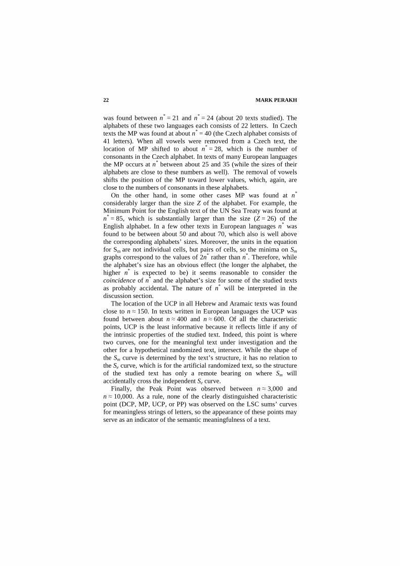
Fig. 2. The measured (Sm, “curve” 1) and expected (Se, “curve” 2) LSC sums for the set of short stories in Russian. The text’s total length is 37000 letters.

For example, in Fig. 2 the expected and measured LSC sums are shown for a text of a set of short stories by the author, published in Russian. We see that despite the drastic difference between the languages (in Fig. 1 it was Hebrew while in Fig. 2 it was Russian), the different text lengths, and the thousands of years between the times of creation of the texts in these two cases, both figures display identical features in regard to the behavior of the variability of letters distribution along the texts.

In both Fig. 1 and Fig. 2, we see the same characteristic point DCP, MP, UCP, and PP, albeit they happen at different values of the cell’s size n. A similar picture, with the distinctive points (DCP, MP, UCP, and PP) was observed for all meaningful texts in all studied languages (except for Finnish and presumably Estonian, where DCP is absent).

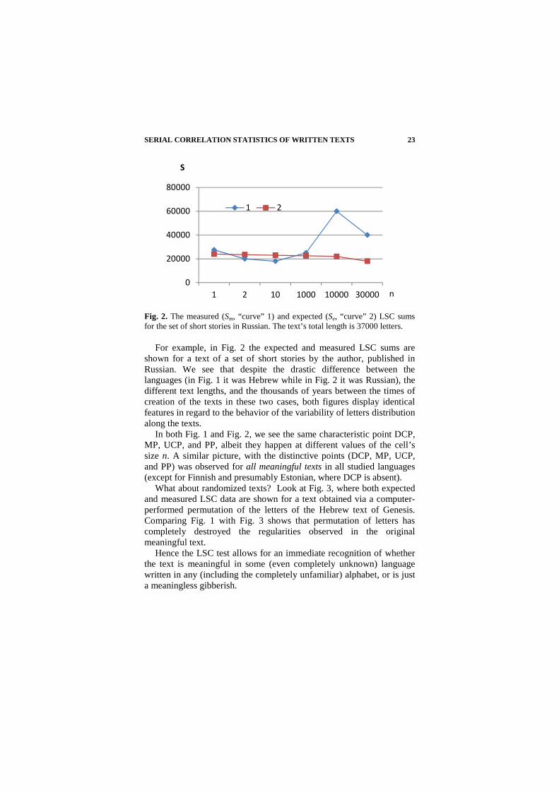
What about randomized texts? Look at Fig. 3, where both expected and measured LSC data are shown for a text obtained via a computer-performed permutation of the letters of the Hebrew text of Genesis. Comparing Fig. 1 with Fig. 3 shows that permutation of letters has completely destroyed the regularities observed in the original meaningful text.

Hence the LSC test allows for an immediate recognition of whether the text is meaningful in some (even completely unknown) language written in any (including the completely unfamiliar) alphabet, or is just a meaningless gibberish.

0

20000

40000

60000

80000

1 2 10 1000 10000 30000

S

n

1 2

MARK PERAKH 24

Fig. 3. Measured (Sm, “curve” 1) and expected (Se, “curve” 2) LSC sums for a text obtained by a random permutation of letters of the Hebrew text of the “Bereshit” (the Book of Genesis). Compare to Fig. 1, where the sums are shown for the same text in its original, non-permuted form.

It should be noted that automatic permutation of the letters of a meaningful text, although converting it into gibberish, does not guarantee its complete randomization. Since the permutation procedure is performed randomly, the number of possible outcomes is very large (it equals N!). The overwhelming majority of the permuted strings are meaningless. However, among the vast multitude of the permuted versions of the same original text there is a certain fraction of strings that accidentally contain blocks of letters possessing a certain degree of order, even including segments of a semantically meaningful text.

Therefore we cannot expect the LSC data for a particular permuted string to coincide with the expected LSC sums calculated by equation (2) for a hypothetical randomized text.

Indeed, as we see in Fig 3, the measured LSC sum for this particular permuted version of the text of Genesis is distinct from the expected LSC sum calculated by equation (2) for a hypothetical randomized text of the same length and with the same letter-frequency distribution. At relatively small cell sizes (up to n ≈ 50) the “curve” of the measured LSC sum is more or less close to the “curve” for the expected sum. This indicates the reasonably high degree of text randomization achieved in this particular permuted string by the letter permutation procedure. At n>50 the curve for the measured LSC sum deviates from the curve for the expected LSC sum, the deviations occurring in a

0

2000

4000

6000

8000

10000

12000

14000

16000

18000

S

n

1 2


25

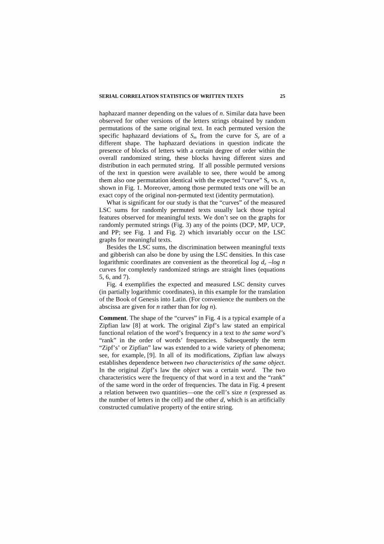
haphazard manner depending on the values of n. Similar data have been observed for other versions of the letters strings obtained by random permutations of the same original text. In each permuted version the specific haphazard deviations of Sm from the curve for Se are of a different shape. The haphazard deviations in question indicate the presence of blocks of letters with a certain degree of order within the overall randomized string, these blocks having different sizes and distribution in each permuted string. If all possible permuted versions of the text in question were available to see, there would be among them also one permutation identical with the expected “curve” Se vs. n, shown in Fig. 1. Moreover, among those permuted texts one will be an exact copy of the original non-permuted text (identity permutation).

What is significant for our study is that the “curves” of the measured LSC sums for randomly permuted texts usually lack those typical features observed for meaningful texts. We don’t see on the graphs for randomly permuted strings (Fig. 3) any of the points (DCP, MP, UCP, and PP; see Fig. 1 and Fig. 2) which invariably occur on the LSC graphs for meaningful texts.

Besides the LSC sums, the discrimination between meaningful texts and gibberish can also be done by using the LSC densities. In this case logarithmic coordinates are convenient as the theoretical log de –log n curves for completely randomized strings are straight lines (equations 5, 6, and 7).

Fig. 4 exemplifies the expected and measured LSC density curves (in partially logarithmic coordinates), in this example for the translation of the Book of Genesis into Latin. (For convenience the numbers on the abscissa are given for n rather than for log n).

Comment. The shape of the “curves” in Fig. 4 is a typical example of a Zipfian law [8] at work. The original Zipf’s law stated an empirical functional relation of the word’s frequency in a text to the same word’s “rank” in the order of words’ frequencies. Subsequently the term “Zipf’s’ or Zipfian” law was extended to a wide variety of phenomena; see, for example, [9]. In all of its modifications, Zipfian law always establishes dependence between two characteristics of the same object. In the original Zipf’s law the object was a certain word. The two characteristics were the frequency of that word in a text and the “rank” of the same word in the order of frequencies. The data in Fig. 4 present a relation between two quantities—one the cell’s size n (expressed as the number of letters in the cell) and the other d, which is an artificially constructed cumulative property of the entire string.

MARK PERAKH 26

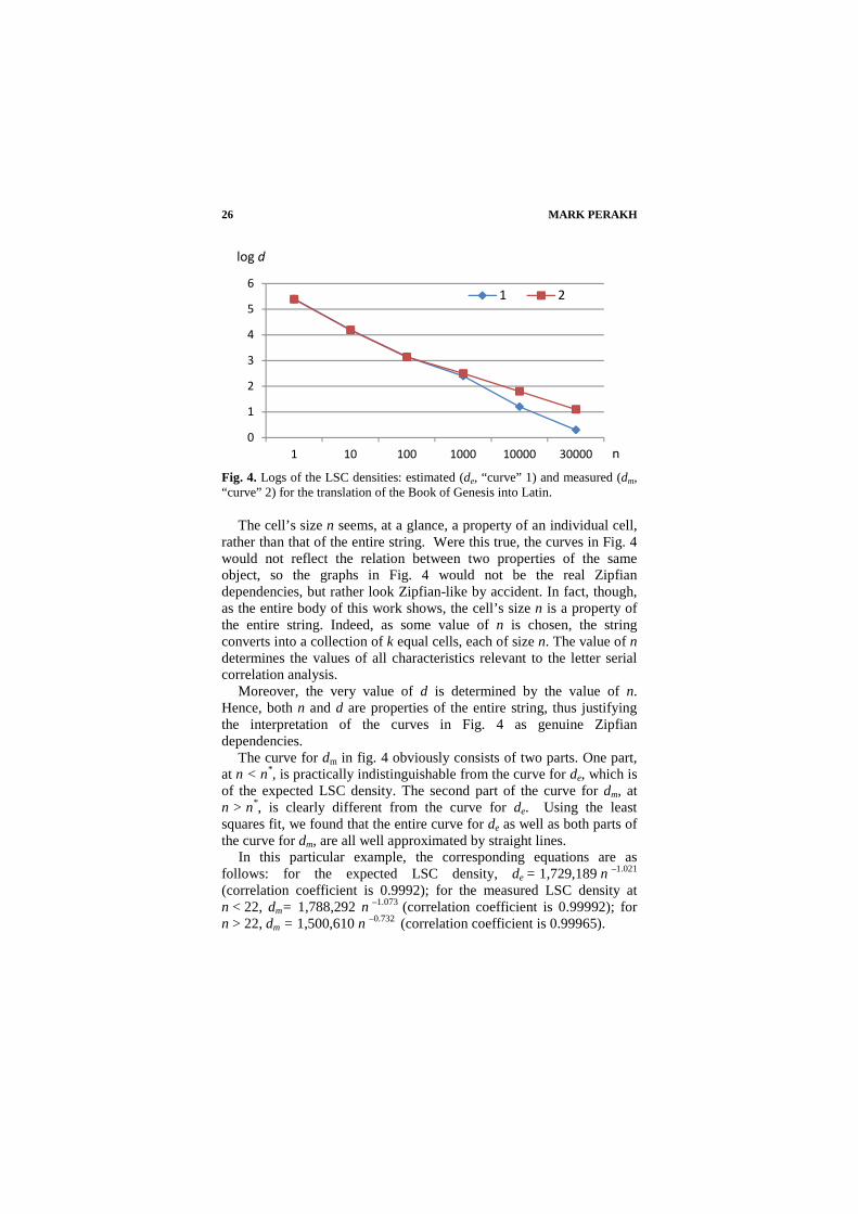
Fig. 4. Logs of the LSC densities: estimated (de, “curve” 1) and measured (dm, “curve” 2) for the translation of the Book of Genesis into Latin.

The cell’s size n seems, at a glance, a property of an individual cell, rather than that of the entire string. Were this true, the curves in Fig. 4 would not reflect the relation between two properties of the same object, so the graphs in Fig. 4 would not be the real Zipfian dependencies, but rather look Zipfian-like by accident. In fact, though, as the entire body of this work shows, the cell’s size n is a property of the entire string. Indeed, as some value of n is chosen, the string converts into a collection of k equal cells, each of size n. The value of n determines the values of all characteristics relevant to the letter serial correlation analysis.

Moreover, the very value of d is determined by the value of n. Hence, both n and d are properties of the entire string, thus justifying the interpretation of the curves in Fig. 4 as genuine Zipfian dependencies.

The curve for dm in fig. 4 obviously consists of two parts. One part, at n < n*, is practically indistinguishable from the curve for de, which is of the expected LSC density. The second part of the curve for dm, at n > n*, is clearly different from the curve for de. Using the least squares fit, we found that the entire curve for de as well as both parts of the curve for dm, are all well approximated by straight lines.

.In this particular example, the corresponding equations are as follows: for the expected LSC density, de = 1,729,189 n –1.021 (correlation coefficient is 0.9992); for the measured LSC density at n < 22, dm= 1,788,292 n –1.073 (correlation coefficient is 0.99992); for n > 22, dm = 1,500,610 n –0.732 (correlation coefficient is 0.99965).

0

1

2

3

4

5

6

1 10 100 1000 10000 30000

log d

n

1 2


27

.The negative exponents in the above equations all differ slightly from 1. As discussed earlier, in the case of the expected LSC densities, the deviations of the exponent from the value of 1 (the latter corresponds to the theoretical hyperbolic curve) reflect the effect of the text’s truncation when the end cell happens to be incomplete and is cast off. In case of a measured LSC density when the shape of dm – n function cannot be theoretically calculated, the deviation of the exponents from unity reflects the difference in the letter-variability distribution between meaningful texts and their permuted versions.

From the above data (which exemplify the similar results obtained for a wide variety of texts in 12 languages) it follows that LSC statistics may be considered a reliable tool for discriminating between meaningful texts, regardless of language and alphabet, on the one hand, and gibberish, on the other.

However, we still need to test whether or not meaningless strings (besides those obtained by permutations of letters of meaningful originals) can sometimes masquerade as meaningful texts by producing LSC data imitating those exemplified in Figures 1 and 2.

To this end various versions of meaningless strings, those possessing a high degree of order as well as those which are highly chaotic, were studied. First, the LSC statistics were applied to strings obtained by various methods of permutation of the meaningful original text.

In one version of the procedure, the words within each paragraph of a meaningful original text were randomly permuted by a computer while the paragraphs themselves stayed in their original places. As long as the doubled cell size (2n) is not exceeding the average word length, the behavior of LSC sums, as could be expected, remained similar to the one observed for meaningful texts. However, as the doubled cell size (2n) becomes larger than the average word length, the LSC sums for the words-within-paragraphs-permuted strings deviate markedly from those for the meaningful texts.

A similar effect was observed in strings obtained by random permutations of the paragraphs of the original meaningful text while the words and letters within the paragraphs remained intact. If paragraphs are short and have been randomly permuted, the overall text becomes in a certain sense meaningless. Since, however, the text within the paragraphs remains intact, each paragraph preserves, within its confines, the structure of a meaningful text.

Therefore, although a string obtained via random permutations of the paragraphs of a meaningful text (keeping the texts within the paragraphs intact) loses its logical consistency and, hence, can be

MARK PERAKH 28

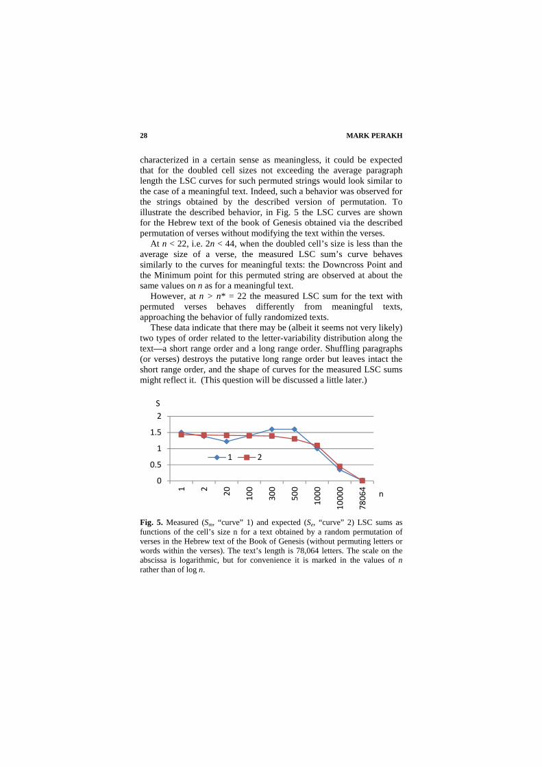
characterized in a certain sense as meaningless, it could be expected that for the doubled cell sizes not exceeding the average paragraph length the LSC curves for such permuted strings would look similar to the case of a meaningful text. Indeed, such a behavior was observed for the strings obtained by the described version of permutation. To illustrate the described behavior, in Fig. 5 the LSC curves are shown for the Hebrew text of the book of Genesis obtained via the described permutation of verses without modifying the text within the verses.

At n < 22, i.e. 2n < 44, when the doubled cell’s size is less than the average size of a verse, the measured LSC sum’s curve behaves similarly to the curves for meaningful texts: the Downcross Point and the Minimum point for this permuted string are observed at about the same values on n as for a meaningful text.

However, at n > n* = 22 the measured LSC sum for the text with permuted verses behaves differently from meaningful texts, approaching the behavior of fully randomized texts.

These data indicate that there may be (albeit it seems not very likely) two types of order related to the letter-variability distribution along the text—a short range order and a long range order. Shuffling paragraphs (or verses) destroys the putative long range order but leaves intact the short range order, and the shape of curves for the measured LSC sums might reflect it. (This question will be discussed a little later.)

Fig. 5. Measured (Sm, “curve” 1) and expected (Se, “curve” 2) LSC sums as functions of the cell’s size n for a text obtained by a random permutation of verses in the Hebrew text of the Book of Genesis (without permuting letters or words within the verses). The text’s length is 78,064 letters. The scale on the abscissa is logarithmic, but for convenience it is marked in the values of n rather than of log n.

0

0.5

1

1.5

2

1 2

20

10

0

30

0

50

0

10

00

10

00

0

78

06

4

S

n

1 2


29

In one more version of permutation, all words of the text were randomly permuted by the computer without permuting letters within the words. In this case the curve for the measured LSC sum was similar to those for meaningful texts as long as the cell’s doubled size 2n was less than the average length of a word. However, when 2n exceeded the average word length, the measured LSC sum behaved differently from the meaningful original, but similar to the curves for the texts randomized by letters permutations.

In another set of control experiments certain artificially created meaningless strings, some with highly ordered and others with chaotic structures were constructed.

One such text was formed by repeating letters of the English alphabet 3,000 times each (first the letter A was repeated 3,000 times, then the letter B, etc.). This string was 63,000 letters long (it contained no segments for the last five letters of the English alphabet). This string was highly ordered so its entropy was close to zero. Since the structure of that text was precisely known, it was possible to theoretically compute its LSC sum and density. The precise formulae for calculating the measured LSC sums and densities for that text are shown in Appendix 2. While the derivations of these formulae are omitted to keep the paper’s size within reasonable limits, the validity of the formulae in question follows from the almost perfect coincidence of the data obtained experimentally and those calculated using these formulae. (Anybody may get the detailed derivation of the formula in question by requesting it from the author.) In Fig. 6 the plot of the LSC density vs. cell size (in log-log coordinates) is shown for the near-zero-entropy string in question. The results of measurements and calculations (conducted for the same set of discrete cell sizes) coincided in this case so closely that the two curves could not be resolved from each other, so the same zigzag-shaped graph in Fig. 6 represents the data for both the measurement and calculation.

This result testifies that we have developed a reasonable understanding of the LSC effect and its relation to the text’s structure. As Fig. 6 shows, the behavior of the LSC statistics in the described near-zero-entropy meaningless string has nothing in common with the behavior of the corresponding quantities for meaningful texts (illustrated in Fig. 4).

Another artificial string was formed by sequentially repeating the English alphabet 2422 times. The entropy of that meaningless string is a little higher than for the previously discussed low entropy texts, but it

MARK PERAKH 30

is still very low. For this text the shape of the Sm – n curve also turned out to be different from the curves for meaningful texts.

One more artificial meaningless string of low entropy was created by first repeating the first half of the English alphabet, i.e. the string ABCDEFGHIJKLM, 17 times; to its end a string was concatenated which consisted of the letters BCDEGFHIJKLMN repeated 17 times; then the letters CDEFGHIJKLMNO, repeated 17 times, followed, etc., until the last substring comprising the second half of the alphabet, also repeated 17 times, completed the text.

Fig. 6. Dependence of both measured (dm) and calculated (dc) Letter Serial Correlation densities on cell size n (in log-log coordinates) for an artificially created highly ordered string 63000 letters long. For convenience, the values on the abscissa are indicated for n rather than for logarithms of n. The upper cusp corresponds to n = m. To the left of the cusp n < m, to the right n > m (in this sample m = 3000).

The procedure was repeated 7 times, so the total length of that text was 20111 letters. Again the Sm – n curve for this highly ordered text was distinctively different from the Sm – n curves for meaningful texts.

Finally, one more meaningless text was made up by randomly hitting the keys on the computer keyboard, trying to avoid favoring any particular letters at the expense of other letters. Unlike the previously discussed artificial texts, which all were substantially ordered and thus had low entropy, this string (which was 10,000 letters long) was prepared with the intention of yielding a highly randomized string thus possessing entropy substantially exceeding that of meaningful texts.

It is known [10, 11] that actions of humans cannot be effected in a genuinely random manner. Despite the strenuous effort to avoid any selectivity in hitting the keyboard buttons, a human operator will

0

1

2

3

4

5

1 5 25

75

25

0

50

0

75

0

17

50

35

00

45

00

log d

n


31

subconsciously but inevitably hit the keys in a not fully random way. As expected, the Sm vs. n curve for the supposedly random string obtained as described revealed certain subconscious selectivity which resulted in a letter frequency distribution different from a fully random string. To a certain extent the letter frequency distribution in the artificial, supposedly random text, indeed turned out to be more uniform than in meaningful texts. (In a perfectly random text the letter frequency distribution is ideally uniform). However, it was not as uniform as it should be in a perfectly random string. Therefore, the Sm – n curve for this artificial high-entropy text displays certain features resembling the data for meaningful texts (for example, a minimum at a certain value n* of a cell size). Although these features are not as clearly evident as they are for meaningful texts, they may cause doubts in regard to the distinction between disordered gibberish and meaningful text insofar as the LSC statistics is applied. While this phenomenon is perhaps of interest for psychology, in our case we needed to determine whether or not the LSC statistics enables us to distinguish between semantically meaningful strings and disordered gibberish of high entropy.

It was found that the plots of specific LSC sums for meaningful texts are more clearly different from those for the artificial high-entropy gibberish than are the plots of Sm sums. Furthermore, the data are distinctively different for meaningful texts and for high-entropy gibberish if a text is divided into halves and the LSC statistics are compared for both halves. In the case of a meaningful text, the exact locations of the MP (i.e. the value of n*) as well as the “depth” of the minimum typically are different for the two halves of the text. On the other hand, in the case of artificial high-entropy gibberish the characteristic points for both halves of the text are almost identical.

As mentioned before, we have also studied texts obtained by removing either all vowels or all consonants from the meaningful texts. These studies have revealed that the “shrunk” texts composed of either only consonants or only vowels preserve all the features of the LSC statistics observed for the original, full versions of the same texts. On the curves of the measured LSC sums for “shrunk” texts all characteristic points DCP, MP, UCP, And PP, discussed earlier, are clearly seen, as they are on the curves for the full, all-letters versions.

(There is a quantitative difference between the LSC sum curves for the full, all-letters versions, and for the “shrunk” only-vowels or only-consonants versions. The removal of all vowels, and even more of all consonants, causes a shift of the MP to lower values of n* and also

MARK PERAKH 32

decreases the “depth of minimum” on those curves.) This points to the deeply intrinsic character of the LSC statistics’ behavior, which is not destroyed even by such a brutal mutilation of texts as the removal of all vowels or of all consonants.

4 Discussion

A detailed discussion of the entirety of our LSC data (which comprise over 300 graphs and scores of tables) cannot be done within the confines of a reasonable paper size. Therefore only a brief discussion of the most salient points will be offered here.

First, we will discuss the nature of the Downcross Point (DCP) observed on measured LSC curves for meaningful texts. The explanation in this case seems to be almost obvious. Recall that the DCP was always observed at the cell’s size between n = 1 and n = 3. In other words, at n = 1, i.e. when the cells contain only one letter each, the measured LSC sum Sm for meaningful texts is slightly larger than the expected LSC sum Se , calculated for a text obtained by permutation of letters of the original meaningful text. This, of course, is expected. Indeed, at n = 1 each cell holds just one letter.

Since the terms in the LSC sum are contributed by pairs of neighboring cells, there are only two possibilities. If both neighboring cells of size n = 1 happen to contain the same letter, the term contributed to the LSC sum by that pair of cells equals zero. If, though, the neighboring cells of that size contain different letters, such pair of cells contributes to the LSC sum a term of 2 (since each of the differing letters in question contributes 1 to the sum; see eq. (1)).

It is easy to figure out that the maximum value of Sm (for n = 1) is observed when no pair of neighboring cells contains the same letter in both cells; the sum is in this case Sm = 2(L – 1) where in this case L = k. Therefore, the more pairs of neighboring cells of size n = 1 hold the same letter, the smaller the LSC sum is. In natural texts doubling of letters is rare; the probability of any pair of neighboring cells of size n = 1 containing the same letter is less than the probability of them holding different letters.

On the other hand, in a randomized texts all letters are almost equally likely to occur in any cell (except of the effect of the letters various frequency, mentioned above), so if in cell j there is letter x, the probability of the same letter x also appearing in cell (j+1) is almost the same as for any other letter, say y, of the alphabet. (Strictly speaking,


33

this assertion is exactly valid only for a perfectly random text, while the calculation of the expected sum was conducted for texts randomized by letter permutations of the original meaningful text; however, the calculation has shown that for not very short texts the quantitative difference between the values of the expected LSC sum for perfectly random texts and for letter-permuted texts is, in practical terms, utterly negligible; therefore the above assertion remains practically valid for our data).

As a result, a randomized text at n=1 usually contains more pairs of neighboring cells with the same letter in each than the original meaningful text. Hence the LSC sum for a randomized text at n = 1 includes more terms equal to zero than the corresponding sum for a meaningful text. This results in a slightly larger Sm at n = 1 for meaningful texts than for randomized strings. At n > 1, when a cell contains more than one letter, the LSC sums, both expected and measured, decrease. Indeed, if cells contain only 1 letter each, each time two neighboring cells hold different letters it means a 100% change of a cell’s content from cell to cell.

If, though, cells contain more than 1 letter each, only a fraction of neighboring cells will have the entire set of letters in each cell different from its neighbor; some other pairs of cells will have only partially different contents, so the change of a cell’s content from cell to cell, on the average, will be less than 100% (i.e. the relative letter variability decreases for n > 1).

The LSC sum is larger when the variability of letters distribution is larger. Since for n > 1 the relative variability decreases, the LSC sums drops. It drops faster for meaningful texts than for randomized ones because in the latter this effect is mitigated by the much larger degree of the overall randomness of the letters distribution. As a result, the descending curve for the gradually decreasing Sm crosses at the DCP the curve for the also decreasing, but at a slower pace, Se.

If the above explanation is correct, certain predictions can be suggested. If a certain language’s orthography requires a frequent doubling of identical letters, for a meaningful text in such a language the measured LSC sum will contain, at n = 1, a slightly larger fraction of pairs of neighboring cells both holding the same letter. Such pairs of cells will contribute to the LSC sum terms equal to zero, and this will result in a decrease of Sm for such a text, making it less than the expected LSC sum Se at n=1. Finnish and Estonian orthography require a frequent doubling of both consonants and vowels. Therefore, based on the above interpretation of the Downcross Point, it could be

MARK PERAKH 34

predicted that for Finnish (and presumably Estonian) texts the measured LSC sum Sm at n = 1 would be no larger than the expected LSC sum Se, as was observed in the variety of other texts, but, on the contrary, would be below the expected LSC sum. This prediction has been fully confirmed experimentally for Finnish texts.

Based on these data one more prediction was made. Italian orthography requires a frequent doubling of consonants but not of vowels. Therefore, for regular meaningful Italian texts no “abnormality” in the mutual location of Sm and Se curves at n = 1 can be expected. Indeed, the LSC curves for Italian texts had the usual configuration wherein at n = 1 the measured LSC sum is slightly larger than the expected LSC sum. It could be expected, though, that in Italian texts stripped of all vowels the frequent doubling of consonants would result in the inversion of the Sm and Se curves at n = 1, as was observed for Finnish texts. This expectation was also fulfilled.

The described observations favor our interpretation of the Downcross Point.

Let us now discuss the Minimum Point. The value of the measured LSC sum Sm is determined by the variability of the letter distribution along the text. Recall that the terms in the Sm sum are calculated for pairs of adjacent cells. The more identical letters happen to occur on the average within the length of 2n, the less Sm is. Obviously, then, the minimum on the Sm – n curve must occur at such cell’s size n*, which corresponds to the minimal average variability of the letters distribution within a segment of the size 2n*.

The observation of the MP means the revelation of what can be referred to as an average Domain of Minimal Letter Variability (DMLV) whose size is 2n* and which exists in all meaningful texts using an alphabetical writing system, regardless of language, style, authorship, alphabet, etc.

While the DMLV is consistently present in all meaningful texts, it is usually absent in gibberish, both of the highly ordered and the highly randomized kinds. (Although in extremely rare cases a string of gibberish may accidentally happen to have a DMLV, this would be an exceptional occurrence, while in meaningful texts it is a rule.)

The statement asserting the consistent existence of a DMLV in all meaningful texts (but its usual absence in gibberish) follows directly from the observation of a distinctive minimum on the Sm – n curves, i.e. it is simply a statement of fact. Its interpretation, although post-factum, does not seem very difficult.


35

It seems reasonable to postulate that the size of a DMLV is related to the size of a text’s segment wherein a certain topic is covered. Then it can be expected that certain words related to that topic occur within that segment more often than on average in the text as a whole. Consequently, a certain set of letters is also expected to occur within that text’s segment more often than in the rest of the text. This means a lower letter variability within the segment in question, which contributes to a smaller value of Sm. The size of a DMLV may be expected to be connected to the average size of a text’s segments covering individual topics.

Our interpretation jibes well with the observed variations between the positions of MP in various texts. For example, the Hebrew and Aramaic texts are written in alphabets each containing only consonants, with the total of 22 letters in the alphabet. On the other hand, the most common European languages use substantially longer alphabets (for example, the English alphabet has 26 letters; the Russian alphabet has 33 letters, while the Czech alphabet has 41 letters). These variations alone necessarily must affect the size of a text’s segment covering a certain topic. However, besides the alphabet’s size, the peculiar ways in which each language structures sentences enhances the variations in the DMLV. Here is a simple illustration. Consider a maxim that came from the ancient Hebrew texts but has become part of many ancient and modern languages. Let us write that maxim in several languages. Start with its original form in Hebrew, which looks like בעיר נביא to be) אין read from right to left). Transliterated into Latin characters, it takes the following form: EIN NVI BIRO. Its length is only 10 letters.

Now let us write the conventional translations of that maxim into English, German, Russian, and Ukrainian. English: There is no prophet in one’s native town. (31 letters, of which 19 are consonants). German: Es gibt kein Prophet in seiner Stadt. (30 letters, of which 19 are consonants). Russian (rendered in Latin letters): Net proroka v otechestve svoem (25 letters, of which 15 are consonants; the combination ch in the Russian alphabet is rendered by one letter). Ukrainian: (rendered in Latin letters): Nema proroka u ridnomu misti. (25 letters, of which 14 are consonants).

Obviously, the Hebrew text requires substantially fewer letters to cover a certain topic, so the DMLV for Hebrew naturally is shorter, than, say, for English or Russian, and the minimum on the Sm “curve” for Hebrew texts appears at lower n (usually about 20–24) than, say, for English texts (typically somewhere about 70 and even more). The unusually large n* = 85 for the UN Sea Trade Treaty also can be

MARK PERAKH 36

interpreted on the same basis: it is written in a heavy legalese; such documents are known for a pedantic verbosity, wherein each statement is expressed with multiple asides and additional clauses, which makes the segment of a text, covering a certain topic, substantially longer than in non-legal texts. This shifts n* to larger values than in non-legalese-written texts.

A natural unit of a semantic content is a sentence. Therefore it may be surmised that the size of a DMLV is somehow related to the average length of a sentence. It hardly could be the length of one sentence, because if 2n* were about one sentence long, n* would be about half a sentence long, and in this case to ensure the minimal letters’ variability, two halves of one sentence would need to contain, on the average, almost the same set of letters, which can hardly be expected. Therefore it seems reasonable to expect that DMLV should comprise several sentences, albeit not too many, so that the set of sentences within the scope of an average DMLV covers a specific narrow subject.

To test that hypothesis we have measured the average lengths of sentences in a variety of texts and compared them with the values of 2n* for these texts.

The value of 2n* varies, depending on languages and specific texts, and usually is between 40 and 170 letters. On the other hand, the average length of a sentence, depending on texts, was found to be between 0.4n* and 1.35n*, the mean value being about 0.8n*. Therefore it can be stated that there is in all meaningful texts an average Domain of Minimal Letter Variability which is between 1.5 and 4.5 sentences long, its average length for a variety of texts being about 2.5 sentences. Apparently that is the average length of a text’s segment typically covering individual subjects and hence containing a limited variety of letters. As the text’s segment becomes longer than, on the average, the length of the DMLV, the subject changes, and with it also the words used, and hence the letter composition becomes more varied, so the measured LSC sum Sm increases above the minimum.

Finally, let us discuss the peak (PP) on the Sm – n curves for meaningful texts. To decipher the nature of that peak special tests have been conducted, in which two types of texts were compared. To this end a long text would be chosen, for example the text of several sequential chapters of Tolstoy’s novel War and Peace in English translation.

The length of the text subjected to the test in one particular case was 180,000 letters. This text was then divided into 18 equal segments of 10,000 letters. The LSC sum was measured for the first segment. Then


37

the text was gradually enlarged by sequentially concatenating additional segments of the same size. The LSC sums were measured at each step of the text’s gradual enlargement. In one set of tests, at each step the added segment was different from the previously concatenated one, being the next segment in the sequence constituting the 180,000 letter-long original text. In another set of tests, at each step the same initial segment was repeatedly concatenated to the string, until the total text comprised 18 identical parts each 10,000 letters long. This way a strong long range order was artificially generated in the tested text, while in the first set of tests the long range order, if such existed, was limited to that existing in the text naturally.

Comparing the two described types of a text, it was found that the LSC sums behave quite differently in the two texts in question. These data indicated that the natural meaningful texts possess no long range order. As the cell size n increases, each cell encompasses a larger chunk of a text. As the length of the text within a cell increases, local violations of order accumulate, until no order can be observed any longer. Since the short range order naturally does not exist anymore for such large values of n, and the long range does not exist in natural meaningful texts anyway, for such large n the text starts behaving similar to a randomized one. For the latter, as the behavior of the expected sum Se shows, the LSC sum always decreases with the increase of n. Hence the Sm – n curve, which is ascending at smaller n, now changes to a descending one, typical of randomized texts. Therefore the peak on the Sm – n curve corresponds to such cell sizes where the LSC type of order in the text completely disappears, and the LSC “curve” follows the behavior typical of random texts. .

5 Conclusion

As the data presented here show, the LSC statistics makes it possible in many cases to reliably distinguish semantically meaningful texts from gibberish, regardless of the alphabet in use, language, style, authorship, etc. The LSC statistics have revealed certain hidden features of the order intrinsic in meaningful texts, as, for example, the existence in all such texts of an average Domain of Minimal Letter Variability. Furtermore, a conection was revealed between the LSC statistics and Zipf’s law.

MARK PERAKH 38

The ancient Hebrew and Aramaic texts display exactly the same behavior regarding the letters’ variability distribution along the text as the text of a Russian newspaper printed in 1988, or as a Shakespeare’s play in English, or as a translation of Genesis into Czech. Languages differ in their vocabulary, grammar, idioms, and alphabets, but somewhere on a deeper level they all seem to follow the same statistical features, which perhaps points to their common origin from a single source.

ACKNOWLEDGEMENTS. Dr. Brendan McKay of the Australia National University, Canberra, Australia, at various periods of time participated in this work, including the preliminary discussion of the idea of LSC, writing the computer programs, used for performing the computation of the LSC data, and running various texts through these programs. The author deeply appreciates Dr. McKay’s contribution. The author is also thankful to anonimous reviewers for pithy comments which served to the paper’s substantial mprovement.

Appendix 1. Derivation of the Formula for Expected Letter Serial Correlation Sum

Recall that Xi,j denotes the number of occurrences of letter xi in a cell number j. Since all cells are of the same length n, we have

Var (Xi,j) = Var (Xi, j+1), (A1)

E(Xi,j) = E (Xi, j+ 1), (A2)

where Var(X) is the variance of X and E is the expected value of X.

Step 1. Variance is calculated [12] as follows :

Var (X) = Е (Х2) – [Е (Х)]2, (A3)

where the first term is the expected square of X and the second term is the square of the expected X.

Consider now the expression Е[(Xi,j + Xi, j+ 1)] 2 which is the expected

square of the sum of the values of X in two sequential cells. From equation (A3) we obtain

Е[(Xi,j + Xi, j+1) 2 ] = Var (Xi,j + Xi,j+ 1) + [E(Xi,j + Xi,j+1)]2. (A4)


39

The expected value of a sum equals the sum of the expected values of the items it comprises [8]. Then, accounting for equation (A2), we obtain from equation (A4):

Е[(Xi,j + Xi, j+1) 2] = Var (Xi,j + Xi, j+1) + 4[E(Xi,j)]

2. (A5)

Now consider the expression

Е[(Xi,j – Xi, j+1)2] + E[(Xi,j + Xi, j+1)

2. (A6)

Replacing the expected value of a sum with the sum of expected values of its constituent items and accounting for (A2), we obtain from (A6) the following set of algebraic transformations:

Е[(Xi,j – Xi, j+1)

2] + Е[(Xi,j + Xi, j+1) 2] =

Е[(Xi,j – Xi, j+1)2 + (Xi,j + Xi, j+1)

2] =

E[(X2i,j

+ X2i,j+ 1

–2Xi,j Xi,j+1+ X2i,j+ X2

i,j+ 1 + 2 Xi,j Xi, j+1] =

E[2 X2i,j+ 2 X2

i, j+1] =E [4 X2i,j] = 4E[X2

i,j]

(A7)

Now subtract (A5) from (A7):

[(Xi,j – Xi, j+1)2] = 4 E [X2

i,j] – 4 [E(Xi,j)]2 – Var (Xi,j + Xi, j+1) (A8)

From equation (A3) we can see that the first two terms in the right side of equation (A8) equal 4Var (Xi,j). Then

Е[(Xi,j – Xi, j+1)2] = 4 Var (Xi,j) – Var (Xi,j + Xi, j+1) (A9)

Comment. If we dealt with perfectly random texts, Xi,j and Xi,j+ 1 would be independent random variables. However, we are deriving formulas for a text randomized by a permutation of the letters of an original meaningful text, so the permuted text is not perfectly random. Unlike for a perfectly random text, the stock of available letters in our case is limited to those letters present in the original meaningful text and in the same numbers. Therefore if a certain letter x occurs in a cell, this decreases the stock of this letter available for the next cell and thus diminishes the probability of x’s occurrence in the next cell. Hence there is a certain negative correlation between Xi,j and Xi,j+ 1 which therefore are not independent variables. In such cases the variance of a sum cannot be replaced with the sum of variances of its constituent items so the variances of both Xi,j and (Xi,j + Xi, j+ 1) must be calculated and inserted into equation (A9) separately. If, though, variables Xi,j and Xi, j+ 1 were independent, the right side of equation (A9) would equal 2Var (Xi,j).

MARK PERAKH 40

Step 2. We have to choose now the distribution function for the quantity Xi,j within a cell. Our options are limited to the choice between the multinomial and hypergeometric distributions [13]. The multinomial distribution is applicable to tests with replacement while the hypergeometric distribution is applicable to tests without replacement. In our case, if a letter, say x, occurs in a cell once, this decreases the probability it will occur again in the same (or the next) cell, because the stock of letters is limited to those actually found in the original meaningful string. Therefore the conditions under which our calculation is conducted meet the definition of tests without replacement. In other words, we postulate the hypergeometric distribution of letters’ frequencies within the cells. (While this choice is theoretically well justified, it has a very little significance in practical terms. As the pertinent calculation shows, the final formulae of Se differ between the cases of a hypergeometric and a multinomial distributions only by the factor of L / (L – 1), where L is the truncated (if need be) length of the text, expressed as the number of letters. Obviously, except for extremely short strings (which are hardly of interest) the above factor is so close to unity that the difference between the formulae for the two listed distributions is utterly negligible; for the sake of theoretical purity we calculate here the expected LSC sum for a hypergeometric distribution.)

For the hypergeometric distribution, the variance is calculated as [12]:

Var (Xi,j) = (L – m) mp (1 – p) / (L – 1), (A10)

where m is the sampling size and p = Mi / L. Recall that Mi is the number of occurrences of the letter xi in the entire string and L is the truncated (if need be) length of the text expressed as a number of letters.

For the first term in the right side of equation (A9) the sampling size m equals the cell size: m = n = L / k. For the second term on the right side of (A9) the sampling size is twice as large: m = 2n = 2L / k. Then we can write for the first term on the right side of (A9):

4 Var (Xi,j) = 4(L – L / k) (1 – Mi / L) Mi / k (L – 1),

or, after a simple algebraic transformation

4 Var (Xi,j) = 4 Mi (L – Mi) (1 – 1 / k) / k (L – 1). (A11)

Similarly, for the second term on the right side of (A9) with its doubled sampling size we obtain


41

Var (Xi,j + Xi, j+1) = 2 (1 – 2 / k) Mi (L – Mi) / k (L – 1). (A11a)

Finally, plugging (A11) and (A11a) into (A9), we find

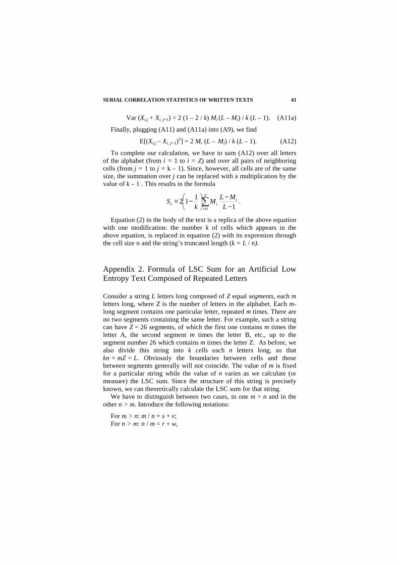
Е[(Xi,j – Xi, j+ 1)2] = 2 Mi (L – Mi) / k (L – 1). (A12)

To complete our calculation, we have to sum (A12) over all letters of the alphabet (from i = 1 to i = Z) and over all pairs of neighboring cells (from j = 1 to j = k – 1). Since, however, all cells are of the same size, the summation over j can be replaced with a multiplication by the value of k – 1 . This results in the formula

∑= −

−

−=Z

i

iie L

MLM

kS

1

.1

112

Equation (2) in the body of the text is a replica of the above equation with one modification: the number k of cells which appears in the above equation, is replaced in equation (2) with its expression through the cell size n and the string’s truncated length (k = L / n).

Appendix 2. Formula of LSC Sum for an Artificial Low Entropy Text Composed of Repeated Letters

Consider a string L letters long composed of Z equal segments, each m letters long, where Z is the number of letters in the alphabet. Each m-long segment contains one particular letter, repeated m times. There are no two segments containing the same letter. For example, such a string can have Z = 26 segments, of which the first one contains m times the letter A, the second segment m times the letter B, etc., up to the segment number 26 which contains m times the letter Z. As before, we also divide this string into k cells each n letters long, so that kn = mZ = L. Obviously the boundaries between cells and those between segments generally will not coincide. The value of m is fixed for a particular string while the value of n varies as we calculate (or measure) the LSC sum. Since the structure of this string is precisely known, we can theoretically calculate the LSC sum for that string.

We have to distinguish between two cases, in one m > n and in the other n > m. Introduce the following notations:

For m > n: m / n = s + v; For n > m: n / m = r + w,

MARK PERAKH 42

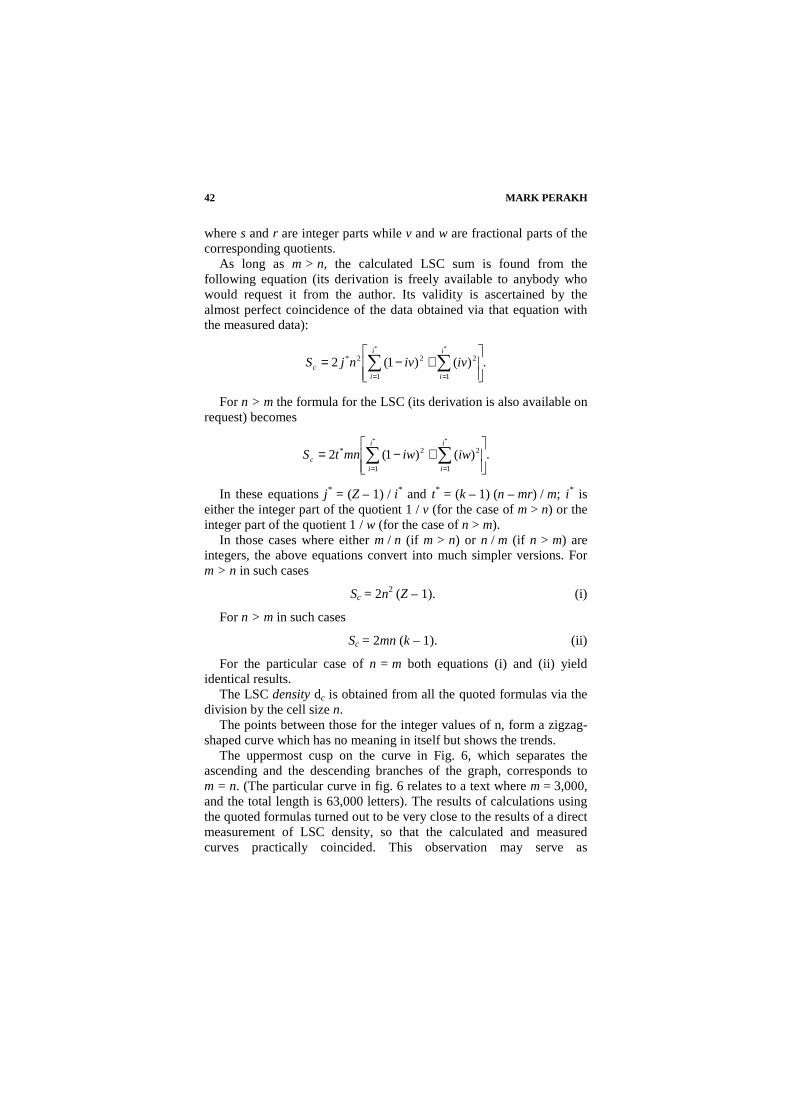
where s and r are integer parts while v and w are fractional parts of the corresponding quotients.

As long as m > n, the calculated LSC sum is found from the following equation (its derivation is freely available to anybody who would request it from the author. Its validity is ascertained by the almost perfect coincidence of the data obtained via that equation with the measured data):

.)()1(2**

1

2

1

22*

+−= ∑∑

==

i

i

i

ic ivivnjS

For n > m the formula for the LSC (its derivation is also available on request) becomes

.)()1(2**

1

2

1

2*

+−= ∑∑

==

i

i

i

ic iwiwmntS

In these equations j* = (Z – 1) / i* and t* = (k – 1) (n – mr) / m; i* is either the integer part of the quotient 1 / v (for the case of m > n) or the integer part of the quotient 1 / w (for the case of n > m).

In those cases where either m / n (if m > n) or n / m (if n > m) are integers, the above equations convert into much simpler versions. For m > n in such cases

Sc = 2n2 (Z – 1). (i)

For n > m in such cases

Sc = 2mn (k – 1). (ii)

For the particular case of n = m both equations (i) and (ii) yield identical results.

The LSC density dc is obtained from all the quoted formulas via the division by the cell size n.

The points between those for the integer values of n, form a zigzag-shaped curve which has no meaning in itself but shows the trends.

The uppermost cusp on the curve in Fig. 6, which separates the ascending and the descending branches of the graph, corresponds to m = n. (The particular curve in fig. 6 relates to a text where m = 3,000, and the total length is 63,000 letters). The results of calculations using the quoted formulas turned out to be very close to the results of a direct measurement of LSC density, so that the calculated and measured curves practically coincided. This observation may serve as


43

confirmation that we have developed a reasonable understanding of both the structure of texts, insofar as their letters variability distribution is in question, and of the working of the LSC statistics.

References

1. R. S. Pindyck, D. L. Rubenfeld. Economic Models and Economic Forecasts. McGrow Hill, NY, 2000.

2. T. J. Bruno & P. D. N. Svoronos. CRC Handbook of Fundamental Spectroscopic Correlation Charts. CRC Press, NJ, 2005.

3. J. Tyrangiel. Why Pop Music Sounds Perfect. Time Magazine, No. 2, 2009. 4. R. J. Solomonoff. A Preliminary Report on a General Theory of Inductive

Inference. Cambridge, MA. Report ZTB138. Zator Co., 1960. 5. A. N. Kolmogorov. Three Approaches to the Quantitative Definition of

Information. Problems of Information Transmission. 1: 1–17, 1965. 6. G. J. Chaitin. Randomness and Mathematical Proof. Scientific American, 5,

232 –238, 1975. 7. P. Vitanyi, “Meaningful information, http://front.math.ucdavis.edu/

cs.CC/0111053, 2000. 8. C. D. Manning. Foundations of Statistical Natural Language Procesing.

MIT Press, Cambridge MA, 1999. 9. N. L. Johnson, S.Kotz and A. W. Kemp. Univariente Discrete Distribution,

2nd ed., John Wiley and Son, NY, 1992. 10. M. Bar-Hillel and W. A. Wagenaar. The perception of randomness.

Advances in Applied Mathematics, 12, 428–454, 1991. 11. G. Keren and C. Lewis (eds). A Handbook for Data Analysis in the

Behavioral Sciences. Hillsdale, NJ: Lawrence Erlbaum, 1993. 12. R. J. Larsen and M. L. Marx. An Introduction to Mathematical Statistics

and its Applications. Englewood, NJ, Prentice-Hall Publishers, 1986. 13. P. Olofsson. Probability, Statistics, and Stochastic Processes. Hoboken, NJ,

Wiley & Son. 2005.

M ARK PERAKH 10106 SAGE HILL WAY ,,

ESCONDIDO, CA 92026, USA, TEL.: 760 751 9932

E-MAIL : <[email protected]>

serial correlation statistics of written texts - gelbukh.com · serial correlation statistics of...

Documents