ser nterfaces with op pin pening iles

1 1/3/2012 University of Minnesota Chemistry Department

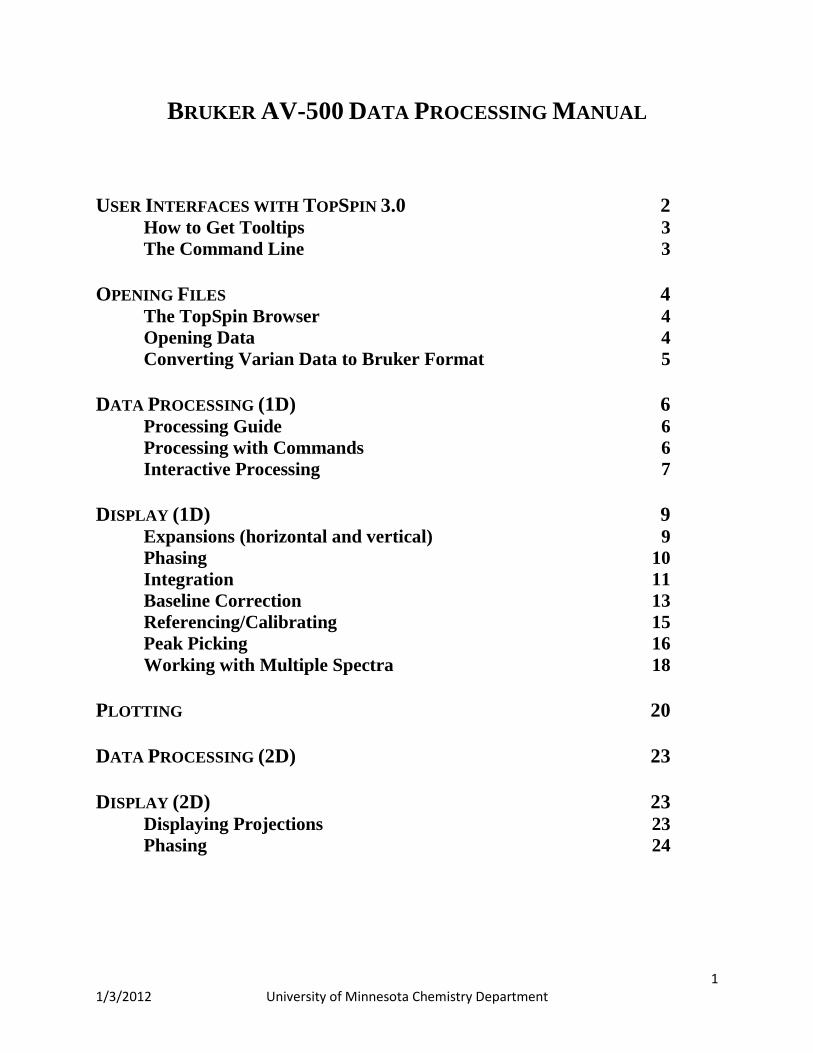
BRUKER AV-500 DATA PROCESSING MANUAL

USER INTERFACES WITH TOPSPIN 3.0 2 How to Get Tooltips 3

The Command Line 3

OPENING FILES 4 The TopSpin Browser 4

Opening Data 4

Converting Varian Data to Bruker Format 5

DATA PROCESSING (1D) 6 Processing Guide 6

Processing with Commands 6

Interactive Processing 7

DISPLAY (1D) 9 Expansions (horizontal and vertical) 9

Phasing 10

Integration 11

Baseline Correction 13

Referencing/Calibrating 15

Peak Picking 16

Working with Multiple Spectra 18

PLOTTING 20

DATA PROCESSING (2D) 23

DISPLAY (2D) 23 Displaying Projections 23

Phasing 24


USER INTERFACES WITH TOPSPIN 3.0 In TopSpin 3.0, there are two user interfaces: classic and a new flow interface. You will be asked which interface you prefer when you open the program. CLASSIC interface:

FLOW interface:

The yellow data button in the upper left corner of the flow interface replaces the File menu in the classic interface.

Help button—calls up PDF manuals

and online documention

Command line

Command line

Data window

Data window


How to Get Tooltips If you hold the cursor over a button on the toolbar, a tooltip will pop up. This is a short explanation of the button’s function. For example, if you hold the cursor over the interactive phase correction button, you will see the following: Classic view: Flow view:

In the flow interface, clicking on the down arrow will bring up a menu of options; clicking on the button itself will execute the command. When in the subroutine, a right-click in the data window will open a pop-up menu that will provide additional options.

Most subroutines will have these buttons: The first exits the subroutine and saves data with the manipulations you have just performed (e.g., phasing, integration). The second exits the subroutine, but does NOT save the changes.

The Command Line The command line is at the bottom of the screen in both interfaces. The main keyboard commands are displayed in parenthesis ( ) (flow) or square brackets [ ] (classic) behind the corresponding menu entries. Some commands require the “.” before the command; others do not. To get help on an individual command, for example ft: + Enter ft? on the command line

How to Retrieve Previously Entered Commands All commands that have been entered on the command line since TOPSPIN was started are stored and can be retrieved. To do that:

+ Hit the (Up-Arrow) key on the keyboard

By hitting this key repeatedly, you can go back as far as you want in retrieving previously entered commands. After that you can go forward to more recently entered commands as follows:

+ Hit the (Down-Arrow) key on the keyboard If you want to execute a series of commands on a dataset, you can enter the commands on the command line separated by semicolons, e.g.: em;ft;apk

If you intend to use the series regularly, you can store it in a macro as follows: + right-click in the command line and choose Save as macro.


OPENING FILES The TopSpin Browser TOPSPIN offers a data browser from which you can browse, select, and open data. The browser dialog offers the following tabs:

• Browser - data browser showing the data directory hierarchy • Last50 - list of the 50 last open datasets • Groups - list of user defined groups of datasets

The browser appears at the left of the TOPSPIN window and can be shown/hidden with Ctrl+d or by clicking the arrow buttons at the upper right of the browser.

How to Open Data If your file is visible in the Browser: + Double-click the file in the Browser or

+ Drag the data file into the data window.

Both of these methods will open your data automatically. If your file is not visible in the Browser (or even if it is): + Select the Start =>Open Dataset button and navigate to your data folder to the “pdata” level. or

+ Click the (classic) or (flow) button in the upper left corner. In the new dialog box, select the first option (Open NMR data stored in standard Bruker format), the Browser type File Chooser and click OK. A file browser appears. Navigate to your data directory and expand it to the level of names, expnos, or procnos (double-click a directory to expand it). Select the desired item and click Display.

Note that the dataset specification consists of the five variable parts of the data directory tree: <dir>\data\<user>\nmr\<dataset name>\<expno>\pdata\<procno>

Example: C:\bio\data\guest\nmr\exam1d_1H\1\pdata\1 On our spectrometer, the files will be in the /opt/data directory.


Converting Varian (VNMR) Data Keyboard command: .vconv + Select Open NMR data stored in special formats and File type VNMR. Navigate to your file and choose [VNMR data conversion]

Enter “1” in EXPNO field. Note: if the containing folder (VNMR-name) has spaces in the name, the data conversion will have problems. Specify the directory (DIR) in which to save the converted data. Select OK.

When you first open a data file, you will see the following:

In this window, the tabs at the top will show the spectrum, processing parameters, acquisition parameters, title, pulse program, integration list, sample information, structure (if available), plot previews, and fid. These buttons are not processing buttons.


DATA PROCESSING Processing Guide The TOPSPIN Processing Guide will guide you through the typical sequence of processing steps. To start the Processing Guide in the Flow interface, type prguide

In the Classic interface, Processing => Data Processing Guide will also open the guide.

The Processing Guide will execute each processing command when you click the

corresponding button. At each step, a dialog box will open, offering you the available options and required parameters. For example, the phase correction button offers various automatic algorithms as well as an option to enter interactive phasing mode.

How to Process Data with Commands Alternatively, any FID or a spectrum displayed in a TOPSPIN window can be processed by: + typing a command on the command line, e.g. ft or

+ invoking a command from the Process menu [Proc. Spectrum] => [Fourier Transform...]

If automatic mode is selected, all functions will execute when you select the option. If automatic mode is not selected, dialog boxes will open with optional parameters that you can adjust.


Processing and analysis commands require certain parameters to be set correctly. Most commands in the Processing menu, like wm, open a dialog box showing the available options and required parameters for that command. Other commands such as em and ft, start

processing immediately. Before you use them, you must set their parameters from the parameter editor. To do that, enter edp or click the ProcPars Tab of the data window. Data can be processed by entering single commands on the command line. A typical 1D processing sequence would be:

em : exponential window multiplication ft : Fourier transform apk : automatic phase correction sref : automatic calibration (referencing) abs : automatic baseline correction

Data can also be processed with so called composite commands. These are combinations of single processing commands. The following composite commands are available.

ef : Exponential multiplication + Fourier transform efp : Exponential multiplication + Fourier transform + phase correction fmc : Fourier transform + magnitude calculation fp : Fourier transform +phase correction gf : Gaussian multiplication + Fourier transform gfp : Gaussian multiplication + Fourier transform + phase correction

1D Interactive Processing + Type .winf in command line. or

+ Click the down arrow in the Proc Spectrum button and select => Window Multiplication [wm], enable Manual window adjustment in the appearing dialog box and click OK.


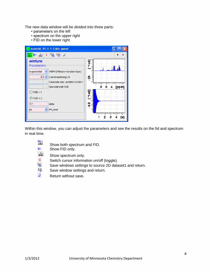
The new data window will be divided into three parts: • parameters on the left • spectrum on the upper right • FID on the lower right

Within this window, you can adjust the parameters and see the results on the fid and spectrum

in real time.

Show both spectrum and FID. Show FID only.

Show spectrum only.

Switch cursor information on/off (toggle).

Save windows settings to source 2D dataset1 and return.

Save window settings and return.

Return without save.


DISPLAY Expansions To expand a certain spectral region: + Click-hold the left mouse button on one side of the region, drag the cursor to the other side and release the mouse.

Buttons for horizontal scaling (zooming): First column is classic view; second column is flow view.

Reset zooming (horizontal scaling) to full spectrum [.hr]

Display the entire spectrum (with baseline position and intensity scaling) [.all]

Zoom in to the center (spectrum) of the displayed region [.zi]

Zoom in/out smoothly

Zoom out from the center (spectrum) or left edge (FID) of the displayed region, decreasing horizontal scaling) [.zo]

Exact zoom via dialog box [.zx]

Toggle interactive zoom mode. When switched off, interactive zooming only selects a horizontal region; baseline position and intensity scaling remain the same. When switched on, interactive zooming draws a box selecting the corresponding area. [.zoommode]

Undo last zoom [.zl]

Retain horizontal and vertical scaling when modifying dataset or changing to different dataset. Global button for all data windows [.keep]

Vertical scaling (intensity)

Increase the intensity by a factor of 2 [*2]

Decrease the intensity by a factor of 2 [/2]

Increase the intensity by a factor of 8 [*8]

Decrease the intensity by a factor of 8 [/8]

Adjusts intensity as you move the mouse cursor within the button

Reset the intensity (baseline positions remains unchanged) [.vr]

Note that vertical scaling can also be changed with the mouse wheel.


Phasing Manually acquired spectra can be phase corrected automatically, with commands like apk or apks or, interactively, in phase correction mode .ph

How to Switch to Phase Correction Mode + Enter .ph on the command line or

+ Click the indicated button in the upper toolbar: Classic view: Flow view: in the Process menu, select:

Putting the mouse on the Adjust Phase button gives you the following tool tip:

Left-clicking on the down arrow gives you additional options:

Right-clicking in the data window gives you a pop-up menu:

The yellow button indicates that you are in phase correction mode. Some buttons will turn orange when they are clicked. As long as a button is orange, it is active. How to Perform a Typical 1D Interactive Phase Correction For a typical 1D phase correction, take the following steps:

1. Click-hold the button and move the mouse within this button (i.e., not on the spectrum itself) until the pivot point (indicated by a red cursor, usually the tallest peak) is exactly in absorption mode.


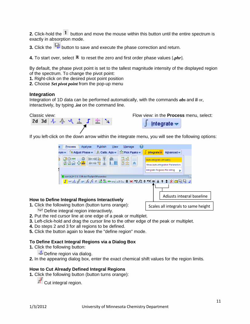
2. Click-hold the button and move the mouse within this button until the entire spectrum is exactly in absorption mode.

3. Click the button to save and execute the phase correction and return. 4. To start over, select to reset the zero and first order phase values [.phr]. By default, the phase pivot point is set to the tallest magnitude intensity of the displayed region of the spectrum. To change the pivot point: 1. Right-click on the desired pivot point position 2. Choose Set pivot point from the pop-up menu

Integration Integration of 1D data can be performed automatically, with the commands abs and li or,

interactively, by typing .int on the command line.

Classic view: Flow view: in the Process menu, select:

If you left-click on the down arrow within the integrate menu, you will see the following options:

How to Define Integral Regions Interactively 1. Click the following button (button turns orange):

Define integral region interactively. 2. Put the red cursor line at one edge of a peak or multiplet. 3. Left-click-hold and drag the cursor line to the other edge of the peak or multiplet. 4. Do steps 2 and 3 for all regions to be defined. 5. Click the button again to leave the "define region" mode. To Define Exact Integral Regions via a Dialog Box 1. Click the following button:

Define region via dialog. 2. In the appearing dialog box, enter the exact chemical shift values for the region limits. How to Cut Already Defined Integral Regions 1. Click the following button (button turns orange):

Cut integral region.

Adjusts integral baseline

Scales all integrals to same height


2. Move the red cursor line into an integral region to the position where it must be cut and click the left mouse button. 3. Do step 2 for each integral region that must be cut. 4. Click on the button again to leave the cut integral mode.

How to Select/Deselect Integral Regions To select/deselect all displayed integral regions:

+ Click the button: button To select a single integral region: 1. Right-click in the integral region. 2. Choose Select/Deselect from the popup menu. Selected integral region turns lime green. To select the next integral region (starts with the first region, then move down the spectrum as you click it)

+ Click the button

To select the previous integral region:

+ Click the button.

To select multiple integral regions:

1. Click the button button to select all integrals 2. Deselect the integrals you don’t want.

How to Delete Integral Regions from the Display

Delete selected integral regions from the display.

Delete all integrals To delete a single integral region from the display: 1. Right-click in the integral region. 2. Choose Delete from the pop-up menu How to Perform Interactive Bias and Slope Correction 1. Select the integral(s) that you want to correct (right-click in the region). We recommend making one big integral region over all peaks in the spectrum, because changing the slope/bias of one integral makes no sense since these are relative integrations.

2. Click-hold and move the mouse until the integral bias is correct.

3. Click-hold and move the mouse until the integral slope is correct.


How to Calibrate/Normalize Integrals Calibrating integrals means setting the value of a reference integral and adjusting all other integrals accordingly. To do that: 1. Right-click in the reference integral region. 2. Choose Calibrate from the pop-up menu. 3. Enter the desired value for the reference integral and click OK

Normalizing integrals means setting the sum of all integrals and adjusting individual integral values accordingly. To do that: 1. Right-click in the reference integral region. 2. Choose Normalize from the pop-up menu 3. Enter the desired sum of all integrals and click OK How to Scale Integrals with Respect to Different Spectra Calibrating and normalizing only affect the current dataset. To scale integrals with respect to a reference dataset, choose lastscale from the right/click pop-up menu. In this way, you can compare integrals of different spectra. Note that this only makes sense for spectra which have been acquired under the same experimental conditions. Integrals can be scaled with respect to the last spectrum that was integrated interactively. To do that: 1. Right-click in the reference integral region. 2. Choose Use Lastscal for Calibration from the pop-up menu. How to Scale Selected Integrals If no integrals are selected, the scaling buttons work on all integrals. However, if integral regions are selected, only those regions will be scaled.

Baseline Correction Baseline correction can be performed with commands like abs or absd or, interactively, as described below. How to Switch to Baseline Correction Mode + Enter .basl on the command line or Classic interface: Flow interface: Select Correct Baseline under Advanced menu.


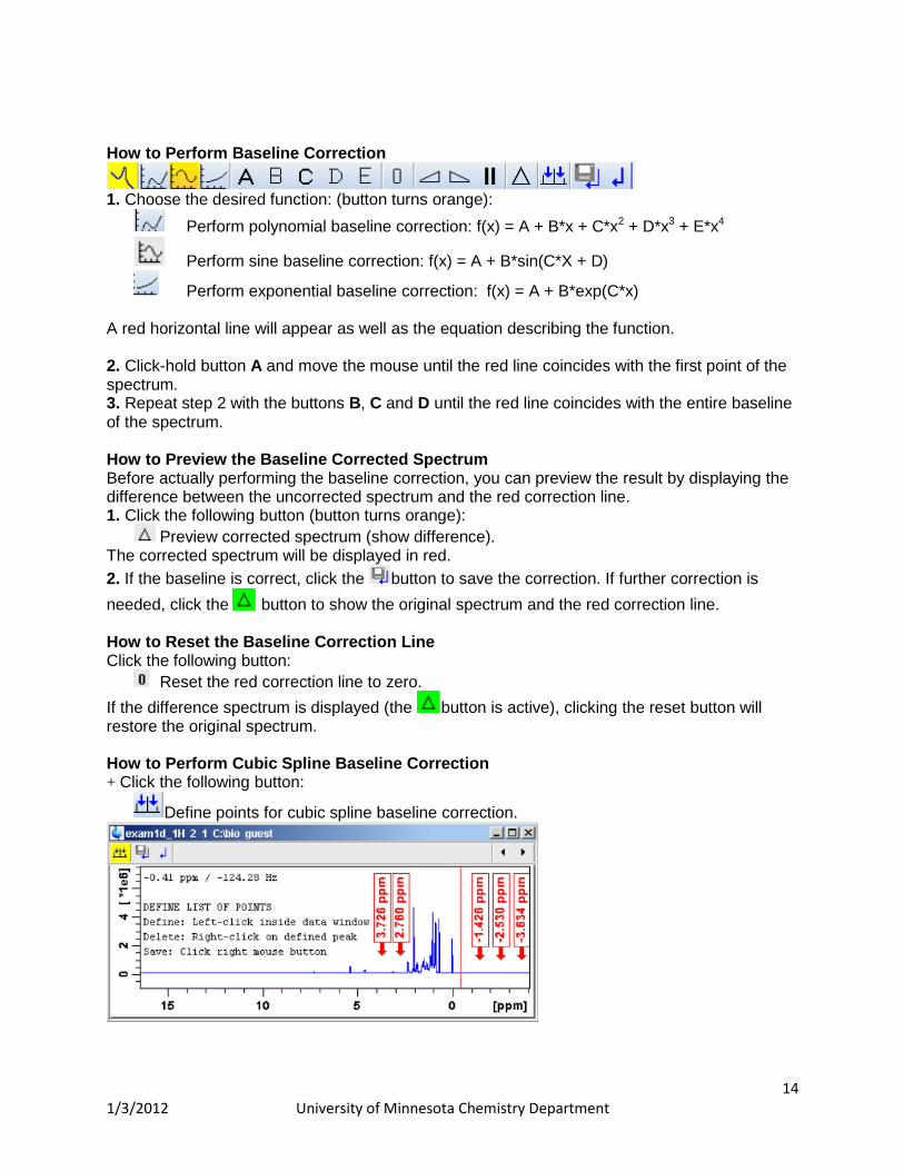
How to Perform Baseline Correction

1. Choose the desired function: (button turns orange):

Perform polynomial baseline correction: f(x) = A + B*x + C*x2 + D*x3 + E*x4

Perform sine baseline correction: f(x) = A + B*sin(C*X + D)

Perform exponential baseline correction: f(x) = A + B*exp(C*x)

A red horizontal line will appear as well as the equation describing the function. 2. Click-hold button A and move the mouse until the red line coincides with the first point of the spectrum. 3. Repeat step 2 with the buttons B, C and D until the red line coincides with the entire baseline of the spectrum. How to Preview the Baseline Corrected Spectrum Before actually performing the baseline correction, you can preview the result by displaying the difference between the uncorrected spectrum and the red correction line. 1. Click the following button (button turns orange):

Preview corrected spectrum (show difference). The corrected spectrum will be displayed in red.

2. If the baseline is correct, click the button to save the correction. If further correction is

needed, click the button to show the original spectrum and the red correction line. How to Reset the Baseline Correction Line Click the following button:

Reset the red correction line to zero.

If the difference spectrum is displayed (the button is active), clicking the reset button will restore the original spectrum. How to Perform Cubic Spline Baseline Correction + Click the following button:

Define points for cubic spline baseline correction.


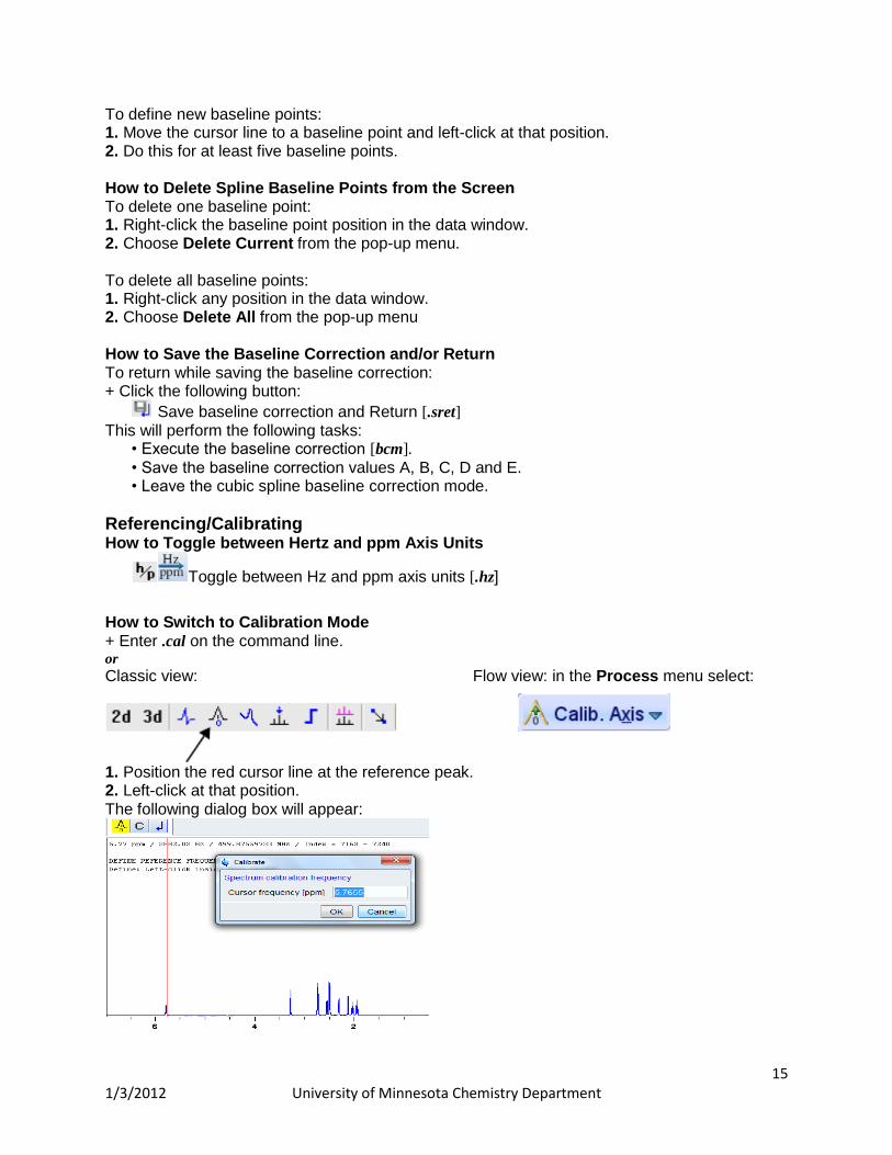
To define new baseline points: 1. Move the cursor line to a baseline point and left-click at that position. 2. Do this for at least five baseline points. How to Delete Spline Baseline Points from the Screen To delete one baseline point: 1. Right-click the baseline point position in the data window. 2. Choose Delete Current from the pop-up menu. To delete all baseline points: 1. Right-click any position in the data window. 2. Choose Delete All from the pop-up menu How to Save the Baseline Correction and/or Return To return while saving the baseline correction: + Click the following button:

Save baseline correction and Return [.sret] This will perform the following tasks:

• Execute the baseline correction [bcm].

• Save the baseline correction values A, B, C, D and E. • Leave the cubic spline baseline correction mode.

Referencing/Calibrating How to Toggle between Hertz and ppm Axis Units

Toggle between Hz and ppm axis units [.hz] How to Switch to Calibration Mode + Enter .cal on the command line. or

Classic view: Flow view: in the Process menu select:

1. Position the red cursor line at the reference peak. 2. Left-click at that position. The following dialog box will appear:


Note that the units (Hz or ppm) correspond to the axis units of the display. 3. Enter the frequency you want to assign to the reference peak. 4. Click OK

The spectrum will be calibrated and re-displayed. TOPSPIN will automatically leave calibration mode.

Peak Picking How to Switch to Peak Picking Mode + Enter .pp on the command line. or

+ Click the indicated button in the upper toolbar: Classic view: Flow view: In the Process menu, select:

New peak picking toolbar

How to Define New Peak Picking Ranges

1. Select 2. Put the cursor at the upper-left corner of a peak picking range and left-click-hold and drag the mouse to the lower-right corner of the range. The peak picking range will be shaded green. The minimum and maximum intensity are set and the peaks in the range are picked and displayed.

3. Repeat for each peak picking range to be defined.

4. Click the button again to leave the "Define peak picking range" mode. Note that the parameters MI and MAXI are set to the lowest minimum and the highest maximum intensity, respectively, of all ranges.


How to Change Peak Picking Ranges 1. Click the following button (button turns orange):

Change peak picking ranges. 2. Put the cursor on one of the edges of the peak picking range. The cursor turns into a double-headed arrow.

3. Left-click-hold and drag the peak range edge to its new position. Click the

button to leave the "Change peak picking range" mode.

How to Define Peaks Manually 1. Click the following button

Define peaks manually. A red vertical line will appear in the data window. 2. Put the red cursor line at the desired peak and click the left mouse button. The peak label will appear at the top of the data window. 3. Repeat step 2 for each peak to be defined.

4. Click the button to leave the "Define peaks" mode.

How to Pick Peaks Semi-Automatically 1. Click the following button:

Define peaks semi-automatically. 2. Move the cursor into the data window. 3. Put the cursor line near the desired peak. 4. Left-click to pick the nearest peak to the right (forward) or

Right-click to pick the nearest peak to the left (backward). 5. Right-click to add the selected peak to the peak list. 6. Click the button to leave the "define peaks semi-automatically" mode.

How to Delete Peaks from the Peak List To delete a specific peak: 1. Right-click on a defined peak. 2. Choose Delete peak under cursor from the pop-up menu

To delete all peaks:

+ Click the button in the data window toolbar. or

+ with no buttons selected, right-click in the spectrum and click Delete All Peaks in the pop-

up menu.


Working with Multiple Spectra How to Superimpose Spectra in Multiple Display Mode TOPSPIN allows you to compare multiple spectra in Multiple Display mode. One feature in this mode is that you can scale and shift each spectrum individually. This allows exact alignment of corresponding peaks of different spectra. If one spectrum is already open, + type .md on the command line and drag in a new dataset or

+ select from the toolbar then drag in a new dataset. If no spectra are currently open, + Hold down the Ctrl key in the browser and click multiple datasets to select them. Choose the

option: Display in new window. In the dialog box, select Open a new window and show the datasets in layered (multiple display) mode.

These buttons in the main TopSpin window move both spectra together.

In the new window shown above, the red (top) spectrum is selected.

allow you to scale and move the selected spectrum. The first three buttons are for scaling, the last two are for moving vertically or horizontally.

Shows the difference between the first and the sum of the other datasets.

Shows the sum of all datasets in the multiple display window.


Saves the displayed sum or difference spectrum. In the appearing dialog box, specify the procno destination of the new file.

How to Display Several Spectra at Once To open several spectra at once: Right-click the datasets in the browser and choose Display, then Display each dataset in its own

window from the pop-up menu. In the upper right of the program, you will now see a 1 and 2 for

the two different spectra. Under the [View] menu, choose your preferred display:

How to Display the Same Spectrum in Different Windows Reopen the same dataset by selecting: File => Reopen This is a convenient way to view various regions of the spectrum simultaneously.

How to Display Spectrum Overview

Select from the toolbar. The full spectrum remains at the top of the data window while you

adjust expansions in the bottom of the data window.


PLOTTING

Under the Publish menu, several options are available: copying the data, printing to a printer, adjusting the plot layout, exporting to PDF, or emailing raw data.

How to Edit the Title Click the Title tab above the spectrum [edti]

How to Print/Plot from the Menu The current data window can be printed as follows: + Click Publish => Print or

+ Enter print or Ctrl+p

All these actions are equivalent; they open the Print dialog box:

How to Print the Integral list 1. Click the Integrals tab of the data window. 2. Enter print or Ctrl+p to print it.

How to Print the Peak list 1. Click the Peaks tab of the data window. 2. Enter print or Ctrl+p

“from screen/CY” takes screen

expansion and adjusts vertical scale

to full scale.


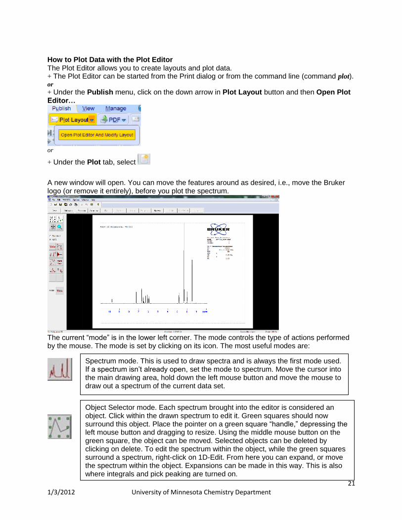
How to Plot Data with the Plot Editor The Plot Editor allows you to create layouts and plot data. + The Plot Editor can be started from the Print dialog or from the command line (command plot). or

+ Under the Publish menu, click on the down arrow in Plot Layout button and then Open Plot Editor…

or

+ Under the Plot tab, select

A new window will open. You can move the features around as desired, i.e., move the Bruker logo (or remove it entirely), before you plot the spectrum.

The current “mode” is in the lower left corner. The mode controls the type of actions performed by the mouse. The mode is set by clicking on its icon. The most useful modes are:

Spectrum mode. This is used to draw spectra and is always the first mode used. If a spectrum isn’t already open, set the mode to spectrum. Move the cursor into the main drawing area, hold down the left mouse button and move the mouse to draw out a spectrum of the current data set.

Object Selector mode. Each spectrum brought into the editor is considered an object. Click within the drawn spectrum to edit it. Green squares should now surround this object. Place the pointer on a green square “handle,” depressing the left mouse button and dragging to resize. Using the middle mouse button on the green square, the object can be moved. Selected objects can be deleted by clicking on delete. To edit the spectrum within the object, while the green squares surround a spectrum, right-click on 1D-Edit. From here you can expand, or move the spectrum within the object. Expansions can be made in this way. This is also where integrals and pick peaking are turned on.


The Annotate (ABC) mode is found by clicking on the Standard button.

To print integral and peak tables in the Plot Editor: 1. Click in “Integrals tab” or in “Peaks tab” 2. Select all peaks or integrals you want 3. Right click in the selection and choose “Copy” in the menu 4. In Plot Editor, choose “Paste”

Editing the spectrum in Plot Editor

Select the spectrum with the button.

The tab in the Plot Editor allows exact expansion (under the [Graph] tab, allows editing of attributes (colors, peak labels) in the spectrum, and the addition of 1D projections onto a 2D plot. For this latter function, choose the [2D Projections] tab, select the location (top, bottom, left, right) for the projection, then use the [Select] button to find your 1D dataset among the currently open datasets.

The button allows intensity and expansion adjustments of the spectrum.

How to make a PDF file. [Publish] – [PDF]


How to email raw data. [Publish] – [Email] If an email client is set up on your computer, you can send the zipped file directly. If not, the zipped file will be stored in your temp folder and you can mail it as an attachment later.

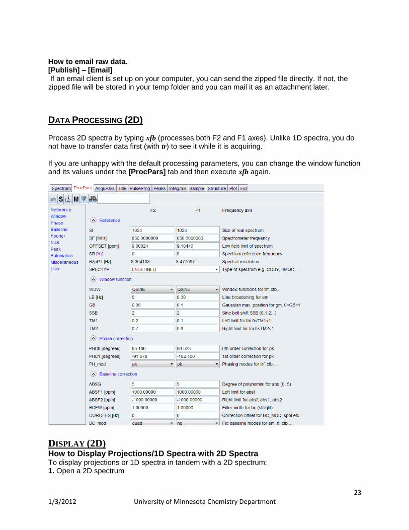
DATA PROCESSING (2D) Process 2D spectra by typing xfb (processes both F2 and F1 axes). Unlike 1D spectra, you do not have to transfer data first (with tr) to see it while it is acquiring. If you are unhappy with the default processing parameters, you can change the window function and its values under the [ProcPars] tab and then execute xfb again.

DISPLAY (2D) How to Display Projections/1D Spectra with 2D Spectra To display projections or 1D spectra in tandem with a 2D spectrum: 1. Open a 2D spectrum


2. If no projections are shown,

+ click the button in the upper toolbar or + enter .pr on the command line.

3. Move the cursor into the F1 or F2 projection area. 4. Right-click and choose one of the options.

+ With External Projection... an existing 1D spectrum can be read (must be processed

first). Enter the filename in the pop-up window. It is often easier to find your data with the [Browse] button than to enter in the filepath. or

+ If no 1D spectrum is available, select Internal Projection and the positive projection will

be calculated and displayed. A right-click in the data area will provide you with the following options:

Unclick the filled blue square in the top right corner if you want to manipulate the 2D spectrum.

How to Perform a Typical 2D Interactive Phase Correction 1. Enter the interactive phase routine by typing .ph

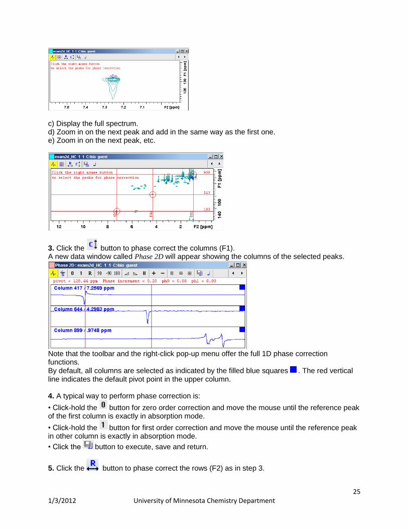
2. Select two or more peaks in different parts of the spectrum. To do that: a) Zoom in on a peak by click-holding the left mouse button and moving the mouse to draw a box around the peak. b) Right-click at the peak position and choose Add from the pop-up menu.


c) Display the full spectrum. d) Zoom in on the next peak and add in the same way as the first one. e) Zoom in on the next peak, etc.

3. Click the button to phase correct the columns (F1). A new data window called Phase 2D will appear showing the columns of the selected peaks.

Note that the toolbar and the right-click pop-up menu offer the full 1D phase correction functions. By default, all columns are selected as indicated by the filled blue squares . The red vertical line indicates the default pivot point in the upper column. 4. A typical way to perform phase correction is:

• Click-hold the button for zero order correction and move the mouse until the reference peak of the first column is exactly in absorption mode.

• Click-hold the button for first order correction and move the mouse until the reference peak in other column is exactly in absorption mode.

• Click the button to execute, save and return.

5. Click the button to phase correct the rows (F2) as in step 3.

ser nterfaces with op pin pening iles

Documents