To ASME Journal of Mechanical Design Revision

Manuscript Number 20302

Sequential Optimization and Reliability Assessment Method for Efficient Probabilistic Design

Xiaoping Du, Assistant Professor

Department of Mechanical and Aerospace Engineering and Engineering Mechanics University of Missouri – Rolla Rolla, Missouri 65409 – 4494

Wei Chen*, Associate Professor

Department of Mechanical Engineering Northwestern University

2145 Sheridan Rd., Evanston, IL 60208-3111, weichen@northwestern.edu *Corresponding Author

Abstract

Probabilistic design, such as reliability-based design and robust design, offers tools for

making reliable decisions with the consideration of uncertainty associated with design

variables/parameters and simulation models. Since a probabilistic optimization often

involves a double-loop procedure for the overall optimization and iterative probabilistic

assessment, the computational demand is extremely high. In this paper, the sequential

optimization and reliability assessment (SORA) is developed to improve the efficiency of

probabilistic optimization. The SORA method employs a single-loop strategy with a

serial of cycles of deterministic optimization and reliability assessment. In each cycle,

optimization and reliability assessment are decoupled from each other; the reliability

assessment is only conducted after the deterministic optimization to verify constraint

feasibility under uncertainty. The key to the proposed method is to shift the boundaries of

violated constraints (with low reliability) to the feasible direction based on the reliability

information obtained in the previous cycle. The design is quickly improved from cycle to

cycle and the computational efficiency is improved significantly. Two engineering

applications, the reliability-based design for vehicle crashworthiness of side impact and

the integrated reliability and robust design of a speed reducer, are presented to

demonstrate the effectiveness of the SORA method.

1 Introduction

Probabilistic design methods have been developed and applied in engineering

design. The typical probabilistic design methods include reliability-based design [1-4]

and robust design [5-9]. Reliability-based design emphasizes high reliability of a design

by ensuring the probabilistic constraint satisfaction at desired levels, while robust design

focuses on making the design inert to the variations of system input through optimizing

mean performance of the system and minimizing its variance simultaneously. One

important task of a probabilistic design is uncertainty analysis, through which we

understand how much the impact of the uncertainty associated with the system input is on

the system output by identifying the probabilistic characteristics of system output. We

then perform synthesis (optimization) under uncertainty to achieve the design objective

by managing and mitigating the effects of uncertainty on system output (system

performance) [10].

In spite of the benefits of probabilistic design, one of the most challenging issues

for implementing probabilistic design is associated with the intensive computational

demand of uncertainty analysis. To capture the probabilistic characteristics of system

performance at a design point, we need to perform a number of deterministic analyses

around the nominal point, either using a simulation approach (for instance, Monte Carlo

simulation) or other probabilistic analysis methods (such as reliability analysis). Many

researches have been concentrating on developing practical means to make probabilistic

design computationally feasible for complex engineering problems.

Our focus in this study is to develop an efficient probabilistic design approach to

facilitate design optimizations that involve probabilistic constraints. Reliability-based

1

design is such type of probabilistic optimization problems in which design feasibility is

formulated as reliability constraints (or the probability of constraint satisfaction). The

conventional approach for solving a probabilistic optimization problem is to employ a

double-loop strategy; the analysis and the synthesis are nested in such a way that the

synthesis loop (outer loop) performs the uncertainty analysis (inner loop for reliability

assessment) iteratively for meeting the probabilistic objective and constraints. As the

double-loop strategy may be computationally infeasible, various techniques have been

developed to improve its efficiency. These techniques can be classified into two

categories: one is through improving the efficiency of uncertainty analysis methods, for

example, the methods of Fast Probability Integration [11] and Two-Point Adaptive

Nonlinear Approximations [3]; the other is through modifying the formulation of

probabilistic constraints, for example, the performance measure approach [12]. A

comprehensive review of various feasibility modeling approaches for design under

uncertainty is provided in Du and Chen [13].

Even though the improved uncertainty analysis techniques and modifications of

problem formulation have lead to improved efficiency of probabilistic optimization, the

improvement is quite limited due to the nature of the double loop strategy. Recent years

have seen preliminary studies on a new type of method – the single loop method [14-16]

that avoids the nested loops of optimization and reliability assessment. In [14], the

reliability constraints are formulated as deterministic constraints that approximate the

condition of the Most Probable Point (MPP) [17], a concept used for reliability

assessment. Since this method does not conduct the expensive MPP search, its efficiency

is very high. However, there is no guarantee that an active reliability constraint converges

2

to its actual MPP; the optimal solution may not satisfy the required reliability. In [15], a

method using “approximately equivalent deterministic constraints” was developed. The

method creates a link between a probabilistic design and a safety-factor based design.

With this method, only deterministic design variables are considered and the uncertainties

can be only associated with (uncontrollable) design parameters. In [16], optimization and

reliability assessment are decoupled in each cycle. In optimization, reliability constraints

are linearlized around the MPPs obtained in the reliability assessment of the previous

cycle. The linearization improves the efficiency of overall optimization but may also lead

to convergence difficulties. Although the single loop strategy appears promising as no

nested synthesis and uncertainty analysis loops are involved , the above methods are

relatively new and their applicability to various design applications is yet to be verified.

In this paper, we present a new probabilistic design method, the Sequential

Optimization and Reliability Assessment (SORA) method that we believe can

significantly improve the efficiency of probabilistic optimization. Our method employs a

single loop strategy which decouples optimization synthesis and uncertainty analysis. As

an integral part of the proposed strategy, we employ the formulation of performance

measure for the reliability constraints along with an efficient inverse MPP search

algorithm. The SORA method has the capability to deal with both deterministic and

random design variables with the presence of random parameters. In this paper, we will

first review a few commonly used strategies of probabilistic design in Section 2. The

review will lay the foundation for our proposed method, SORA, introduced in Section 3.

In Section 4 two engineering examples are used to illustrate the effectiveness of the

proposed method. Section 5 is the closure, which highlights the effectiveness of the

3

proposed method and provides discussions on its applicability under different

circumstances.

2 Probabilistic Optimization Strategies

In this section, we present two commonly used formulations under the double-loop

strategy, which lays the foundation for our proposed method. Results from these two

formulations are compared with those from our proposed method in case studies.

2.1 Double-Loop Strategy with Probabilistic Formulation

A typical model of a probabilistic design is given by:

Minimize: ) , ,( PXdfDesign Variable } ,{ xµd=DV (1)

Subject to: Prob{ ( , , ) 0}i ig R≤ ≥d X P , i = 1, 2, …, m,

where f is an objective function, d is the vector of deterministic design variables, X is the

vector of random design variables, P is the vector of random design parameters, gi(d, X,

P) (i = 1, 2, …, m) are constraint functions, Ri (i = 1, 2, …, m) are desired probabilities of

constraint satisfaction, and m is the number of constraints. The design variables are d and

the means (µx) of the random design variables X. Note that the following rules of

symbols are used to differentiate the representation of random variables, deterministic

variables, and vectors. A capital letter is used for a random variable, a lower case letter

for a deterministic variable or a realization of a random variable, and a bold letter is used

for a vector. For example, X stands for a random variable and x for a deterministic

variable or a realization of random variable X; X denotes a vector of random variables

while x denotes a vector of deterministic variables.

4

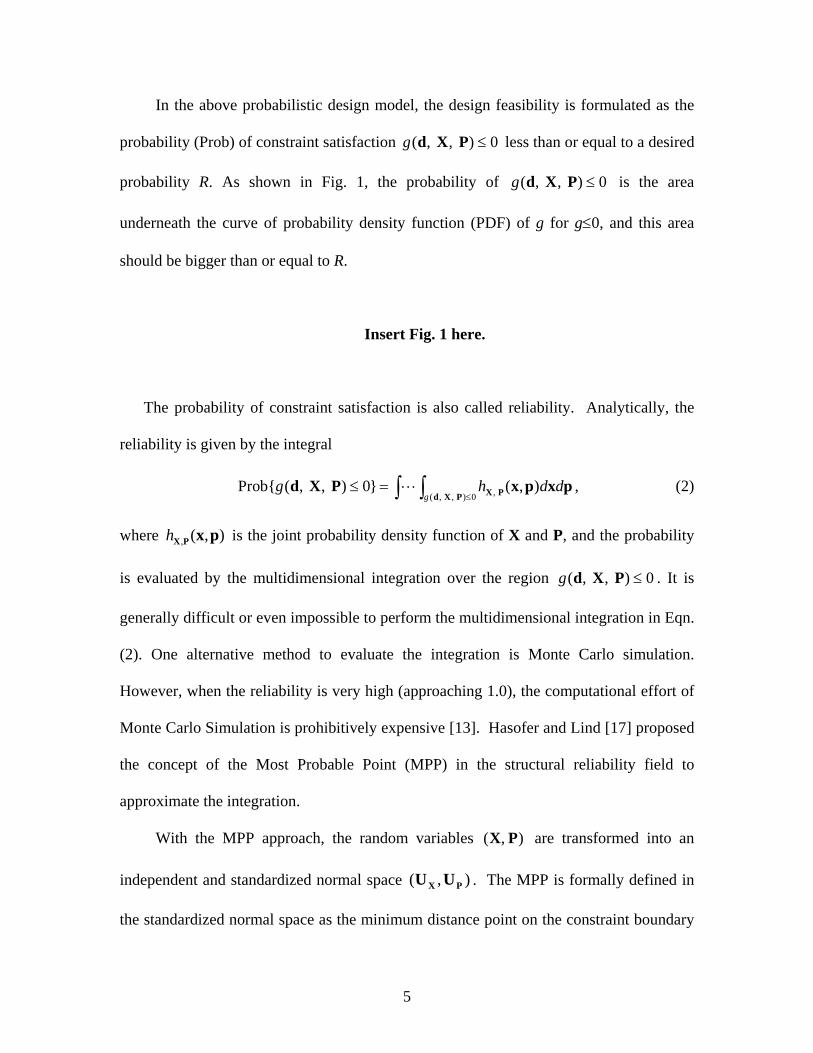
In the above probabilistic design model, the design feasibility is formulated as the

probability (Prob) of constraint satisfaction ( , , ) 0g ≤d X P less than or equal to a desired

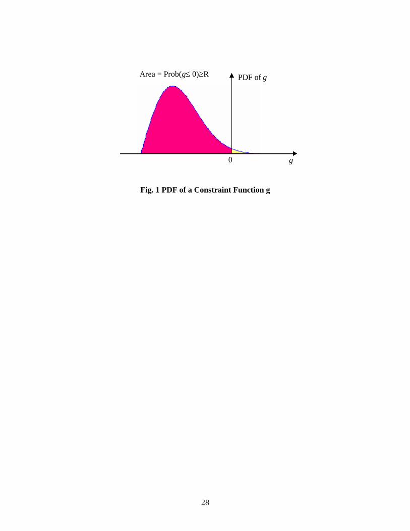
probability R. As shown in Fig. 1, the probability of is the area

underneath the curve of probability density function (PDF) of g for g≤0, and this area

should be bigger than or equal to R.

( , , ) 0g ≤d X P

Insert Fig. 1 here.

The probability of constraint satisfaction is also called reliability. Analytically, the

reliability is given by the integral

, (2) , ( , , ) 0Prob{ ( , , ) 0} ( , )

gg h

≤≤ = ∫ ∫ X Pd X P

d X P x p x pL d d

where is the joint probability density function of X and P, and the probability

is evaluated by the multidimensional integration over the region . It is

generally difficult or even impossible to perform the multidimensional integration in Eqn.

(2). One alternative method to evaluate the integration is Monte Carlo simulation.

However, when the reliability is very high (approaching 1.0), the computational effort of

Monte Carlo Simulation is prohibitively expensive [13]. Hasofer and Lind [17] proposed

the concept of the Most Probable Point (MPP) in the structural reliability field to

approximate the integration.

, ( , )hX P x p

( , , ) 0g ≤d X P

With the MPP approach, the random variables are transformed into an

independent and standardized normal space . The MPP is formally defined in

the standardized normal space as the minimum distance point on the constraint boundary

) ,( PX

),( PX UU

5

0) , ,() , ,( == PX UUdPXd gg to the origin. The minimum distance β is called reliability

index. When the First Order Reliability Method (FORM) [17] is used, the reliability is

given by

Prob{ ( , , ) 0} ( ),g β≤ = Φd X P (3)

where is the standard normal distribution function. Finding the MPP and the reliability

index is a minimization problem, which usually involves an iterative search process.

Therefore, the reliability assessment itself is an optimization problem. For details about

the MPP based method, refer to [18].

Φ

When the probability formulation in design model (1) is directly used to solve the

problem, the method is called “double-loop method with probability formulation”

(DLM_Prob) [12, 19, 20]. The efficiency of this type of method is usually low since it

employs nested optimization loops to first evaluate the reliability of each probabilistic

constraint and then to optimize the design objective subject to the reliability

requirements.

2.2 Double-Loop Strategy with Percentile Formulation

An equivalent model to (1) is given by [12, 15, 21]

Minimize: ) , ,( PXdf} ,{ xµd=DV (4)

Subject to: ( , , ) 0Rig ≤d X P , i = 1, 2, …, m,

where is the R- percentile of , namely, Rg ) , ,( PXdg

Prob{ ( , , ) }Rg g R≤ =d X P (5)

6

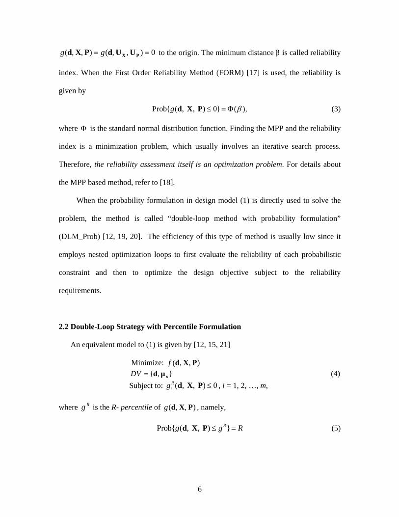
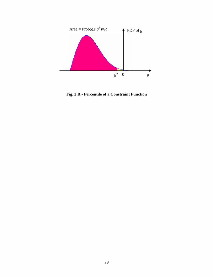
Eqn. (5) indicates that the probability of less than or equal to the R-

percentile is exactly equal to the desired reliability R. The concept is demonstrated in

Fig. 2. If the shaded area is equal to the desired reliability R, then the left ending point

on the g axis is called the R - percentile of function g. From Fig. 2 we see that, if

, it indicates that

) , ,( PXdig

Rg

Rg

0Rg ≤ Prob{ ( , , ) 0}ig R≤ ≥d X P , i.e., the constraint is feasible.

Therefore, the original constraints that require the reliability assessment are now

converted to constraints that evaluate the R -percentile.

Insert Fig. 2 here.

The percentile can be evaluated by the inverse MPP method. When using

FORM, given the desired reliability R, the reliability index β is first calculated by

Rg

(6) )(1 R−Φ=β

The inverse MPP problem is formulated as shown in the following minimization

model,

(7) ⎩⎨⎧

= ,)( subject to)( minimize

2/1 βUUU

T

g

where . ) ,( PX UUU =

Using an inverse MPP search algorithm, the optimum solution MPP can be

identified and the R percentile is evaluated by

MPPu

. (8) ) ,()( MPPMPPMPPR ggg pxu ==

To some extent, the evaluation of Eqn. (8) can be viewed as deterministic by

substituting the MPP values ( and in the original random space) directly into MPPx MPPp

7

the g function. Since applying the inverse MPP method also involves iterative

procedures, we call the method for solving model (4) “the double-loop method with

percentile formulation” (DLM_Per). It is also called performance measure approach

(PMA) in [12, 21].

To distinguish the type of function evaluations for the probabilistic constraints

(Eqns. (3) or (8)) from those for the original constrain functions , we call the

function evaluations for the reliabilities

) , ,( PXdg

Prob{ ( , , ) 0}ig ≤d X P or the R-percentile

“probabilistic function evaluations” and those for the

original function “the performance function evaluations” or simply “the

function evaluations”.

) ,()( MPPMPPMPPR ggg pxu ==

) , ,( PXdg

For both DLM_Prob and DLM_Per, to fulfill the probabilistic optimization, the

outer loop optimizer calls the objective function and each probabilistic constraint

repeatedly. Therefore, the total number of function evaluations can be very huge. For

instance, assume that the outer optimization loop needs 100 probabilistic function

evaluations and that there are 10 probabilistic constraints, if each probability evaluation

needs 50 function evaluations on average, the total number of function evaluations would

be 100×10×50=50,000!

3 Sequential Optimization and Reliability Assessment (SORA) Method

To improve the efficiency of probabilistic optimization, we adopt in this work the

strategy of “serial single loops” [14-16] to develop a sequential optimization and

reliability assessment (SORA) method. Our proposed method is different from the

8

existing single loop methods in the way we establish equivalent deterministic constraints

from the probabilistic constraints. We also employ an efficient inverse MPP search

algorithm as an integral part of the proposed procedure.

3.1 The Measures Taken in Developing the SORA Method

In developing the SORA method, several measures have been taken, including

evaluating the reliability only at the desired level (R-percentile), using an efficient and

robust inverse MPP search algorithm, and employing sequential cycles of optimization

and reliability assessment.

(1) Evaluating the reliability only at the desired level (R-percentile)

It is noted that in probabilistic optimization, the closer the reliability

is to 1.0, the more computational effort is required. For using the

MPP based methods, the higher reliability means larger search region in the standardized

normal space to locate the MPP and it is very likely that more function evaluations are

required. In probabilistic optimization with multiple constraints, some constraints may

never be active and their reliabilities are extremely high (approaching 1). Although these

constraints are the least critical, the evaluations of these reliabilities will unfortunately

dominate the computational effort in the probabilistic design process if the DLM_Prob

strategy (Section 2.1) is employed. Our solution to this problem is to perform the

reliability assessment only up to the necessary level, represented by the desired reliability

R.

P{ ( , , ) 0}ig ≤d X P

To this end, we use the percentile formulation for probabilistic constraints with the

SORA method. Based on Eqn. (8), the design model (5) of DLM_Per is rewritten as

9

Minimize: ) ,( xµdf} ,{ xµd=DV (9)

Subject to: ( , , ) 0i MPPi MPPig ≤d x p , i = 1, 2, …, m

This model establishes the equivalence between a probabilistic optimization and a

deterministic optimization since the original constraint functions are

used to evaluate design feasibility using the inverse MPPs corresponding to the desired

reliabilities R

) , ,( MPPiMPPiig pxd

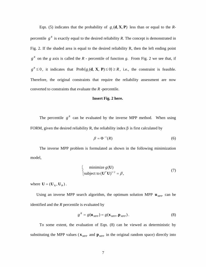
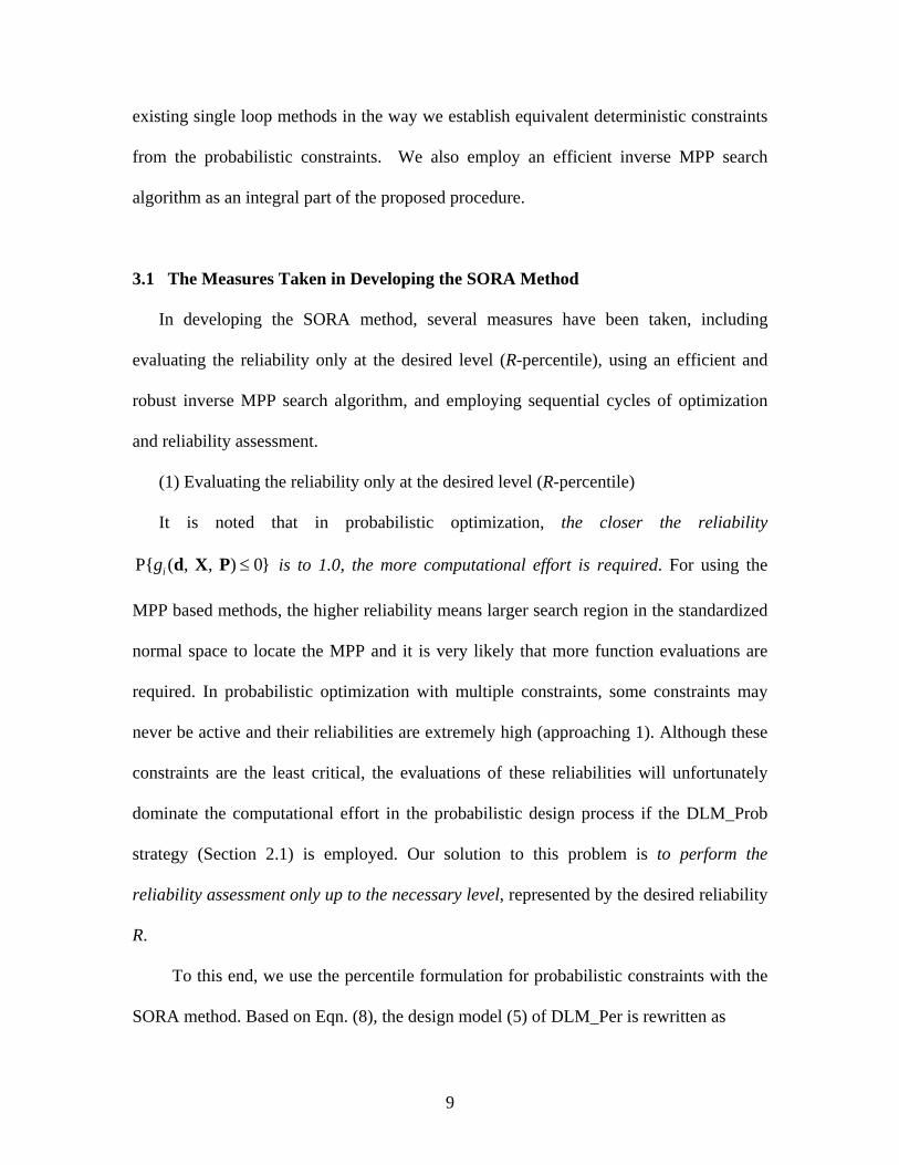
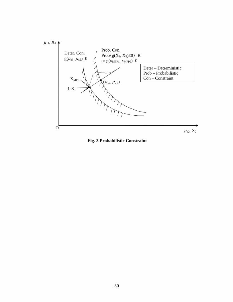
i. Fig. 3 is used to further explain how a probabilistic constraint is

converted to an equivalent deterministic constraint. In this illustrative example, only two

random design variables X1 and X2 are involved; there are no random parameters P. Two

coordinate systems are plotted in Fig. 3; one is the design space (the space composed of

design variables µx1 and µx2), and the other is the random space (X1 and X2). If we do not

consider any uncertainty, curve 1 2( , ) 0x xg µ µ = is the constraint boundary in the

deterministic design. When we consider uncertainty, the constraint boundary

becomes { }1 2Prob g( , ) 0X X ≤ = R . Since in a probabilistic design, the required reliability

R is often much higher than the reliability achieved by a deterministic design, the

constraint of a probabilistic design is stricter than a deterministic design. Geometrically,

the feasible region of a probabilistic design is narrower than the one of a deterministic

design; in other words, the feasible region of a probabilistic design is a reduced region in

comparison with a deterministic feasible design. Determining the probabilistic constraint

boundary { }1 2Prob g( , ) 0X X ≤ = R needs a reliability analysis. Since

{ }1 2Prob g( , ) 0X X ≤ = R is equivalent to ( , , ) 0MPP MPPg =d x p , where (xMPP, pMPP) is

the inverse MPP point, the evaluation of a probabilistic constraint at design point (µx1,

µx2) is equivalent to evaluating the deterministic constraint at the inverse MPP point, i.e.,

10

) , ,( MPPMPPg pxd . As shown in Fig. 3, to maintain the probabilistic constraint

, the Inverse MPP corresponding to the design point (µ0) , ,( =MPPMPPg pxd x1, µx2) on the

probabilistic constraint boundary should be exactly on the deterministic constraint

boundary 1 2( , ) 0x xg µ µ = . Therefore, to maintain the design feasibility, the inverse MPP

of each probabilistic constraint should be within the deterministic feasible region.

Insert Fig. 3 here.

(2) Using an efficient and robust inverse MPP search algorithm

In SORA, we employ an efficient MPP based percentile evaluation method (inverse

MPP search algorithm) of which principle is detailed in [22]. This new inverse MPP

search algorithm combines several techniques, such as using the steepest decent direction

as the search direction, performing an arc search if no progress is made along the steepest

decent direction, and adopting the adaptive step size for numerical derivative evaluation.

This search algorithm is considered robust since it is suitable for any continuous

constraint functions (including non-concave and non-convex functions) and continuous

distributions of uncertainty.

(3) Employing sequential cycles of optimization and reliability assessment

It is noted that in a probabilistic design, most of the computations are used for

reliability assessments. Therefore, to improve the overall efficiency of probabilistic

optimization we need to reduce the number of reliability assessments as much as

possible. The essence is to move the design solution as quickly as possible to its optimum

so as to reduce the needs for locating MPPs. To achieve this, SORA employs a serial of

cycles of optimization and reliability assessment. Each cycle includes two parts, one part

is the (deterministic) optimization and another part is the reliability assessment. The

11

reliability assessment refers to the evaluation of R-percentile corresponding to a given

reliability R. In each cycle, at first we solve an equivalent deterministic optimization

problem, which is formulated by the information of the inverse MPPs obtained in the last

cycle. Once the design solution is updated, we then perform reliability assessment to

identify the new inverse MPPs and to check if all the reliability requirements are

satisfied. If not, we use the current inverse MPPs to formulate the constraint for the

deterministic optimization in the next cycle in which the constraint boundary will be

shifted to the feasible region by changing the locations of design variables. Using this

strategy, the reliability of constraints improves progressively and the solution to a

probabilistic design can be found within a few cycles, and the need for searching MPPs

can be reduced significantly. Detailed flowchart and procedure are provided in Section

3.2.

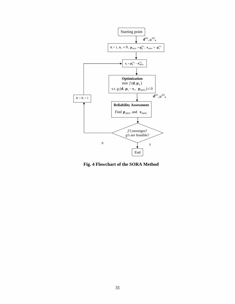
3.2 SORA Flowchart and Procedure

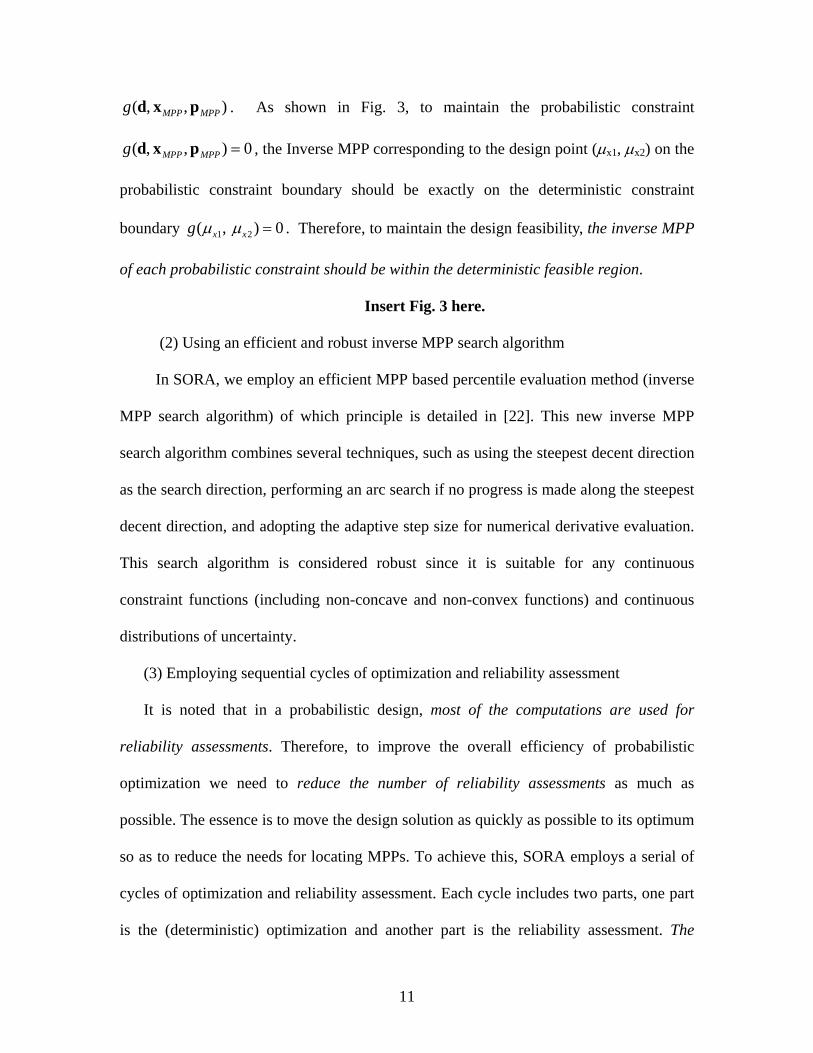
The flowchart of the SORA method is provided in Fig. 4. For the deterministic

optimization in the first cycle, since there is no information about the MPPs, the values of

xMPP and pMPP are set as the means of the random design variables and the random

parameters, respectively. The following is the deterministic optimization model in the

first cycle of probabilistic optimization,

Minimize: ( , , )f x pd µ µ} ,{ xµd=DV (10)

Subject to: ( , , ) 0ig ≤x pd µ µ , i= i = 1, 2, …, m

Insert Fig. 4 here.

12

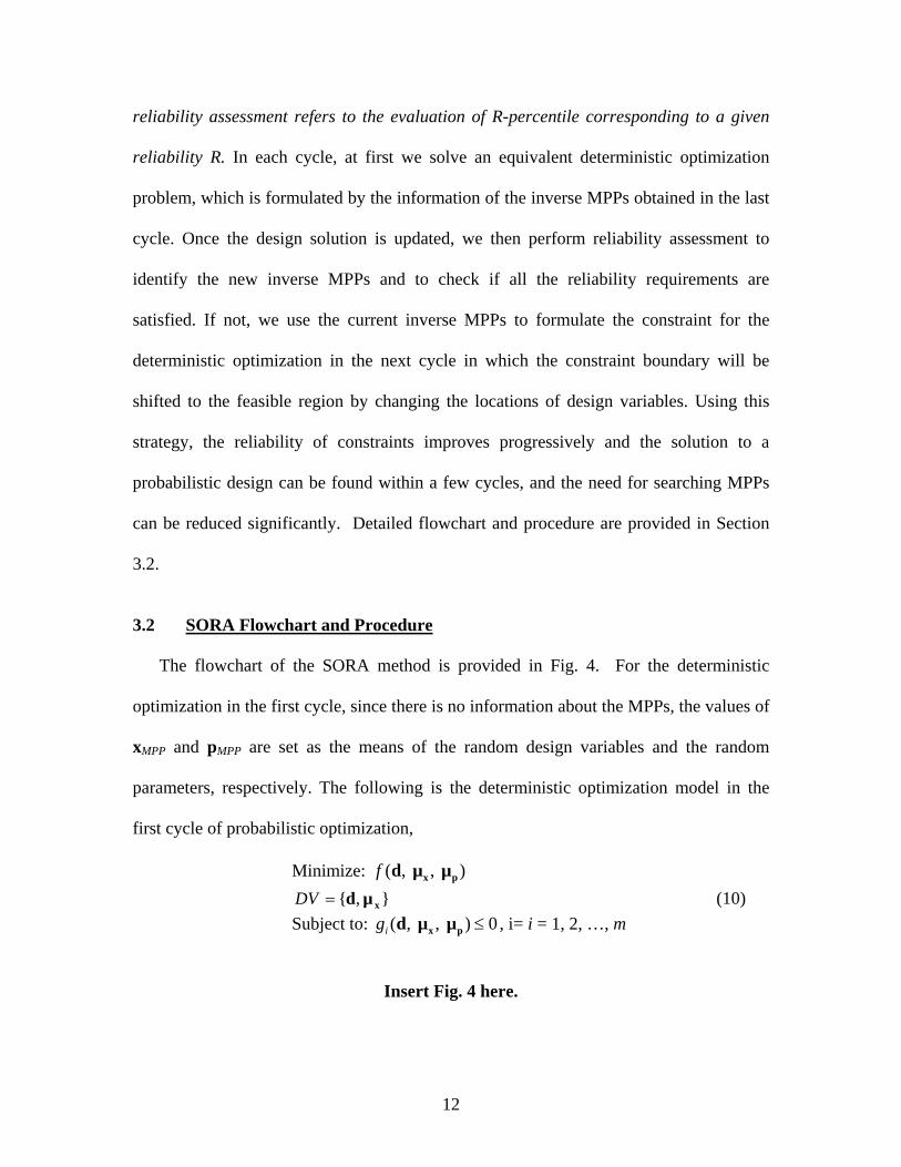
To demonstrate the strategy of separating (deterministic) optimization and

reliability assessment while ensuring both segments work together to bring the design

solution quickly to a feasible and optimal solution, we use the same illustrative plot (no

deterministic design variables d and random parameters P) as shown in Fig. 3 for

demonstration. We start our explanation for the first cycle and then extend the same

principle to the kth cycle. In the first cycle, after solving model (10) (deterministic

optimization), some of the constraints may become active. For an active constraint g, the

optimal point (1) (1) (1)1 2 ( , x x x )µ µ=µ is on the boundary of the deterministic constraint

function . When considering the randomness of X, as seen on the graph (Fig.

5), the actual reliability (probability of constraint being feasible) is only around 0.5. After

the deterministic optimization, the reliability assessment is implemented at the

deterministic optimum solution

) , ( px µµg

(1) (1) (1)1 2( , x x x )µ µ=µ to locate the (inverse) MPP that

corresponds to the desired R level. As one can expect, the MPP (1)MPPx of constraint

will fall outside (to the left of) the deterministic feasible region. From our

discussion in Section 3.1, we know that to ensure the feasibility of a probabilistic

constraint, the inverse MPP corresponding to the R percentile should fall within the

deterministic feasible region. Therefore, when establishing the equivalent deterministic

optimization model in Cycle 2, the constraints should be modified to shift the MPP at

least onto the deterministic boundary to help insure the feasibility of the probabilistic

constraint. If we use s to denote the shifting vector, the new constraint in the

deterministic optimization of the next cycle is formulated as

) , ( px µµg

( )g 0− ≤xµ s (11)

13

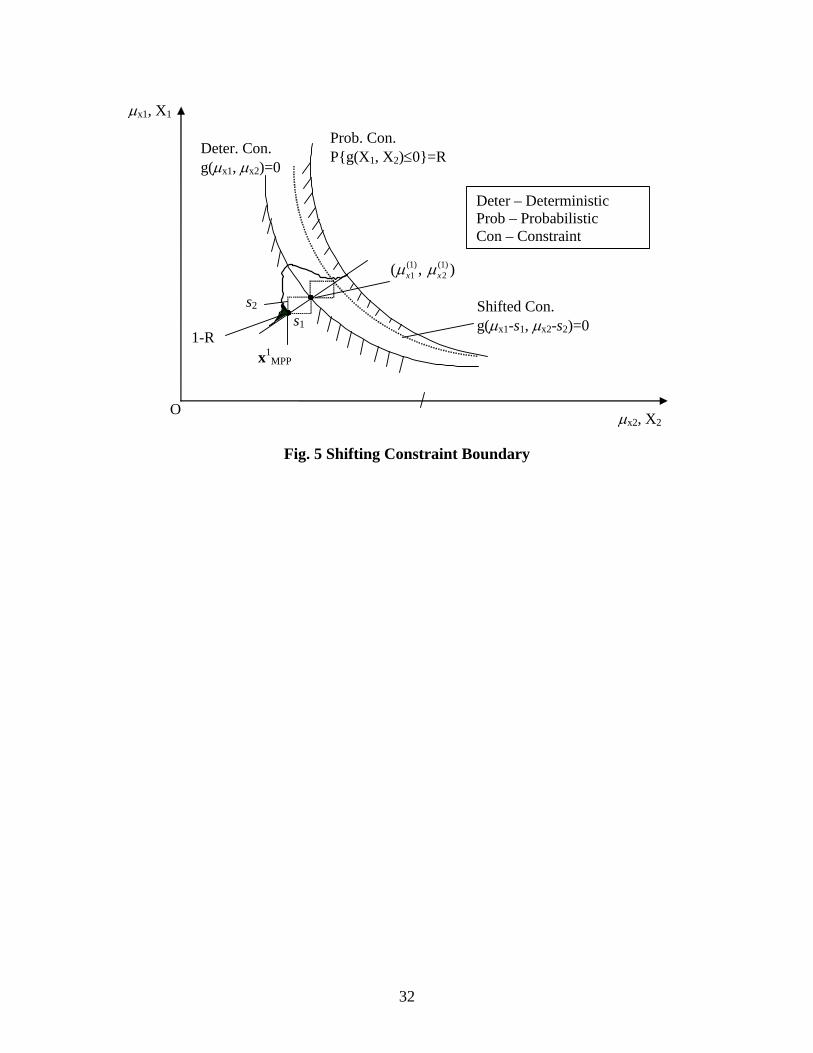
Insert Fig. 5 here.

From Fig. 5, to ensure the MPP onto the deterministic boundary, we derive the

shifting vector as

(1) (1) (1) (1) (1)1 2 1 1 2 2( , ) ( , )MPP x MPP x MPPs s µ x µ x= = − = − −xs µ x . (12)

Correspondingly, Eqn. (11) indicates that the location of the design variables ( )

in the deterministic optimization model needs to move further to the boundary of the

probabilistic constraint to ensure feasibility under uncertainty. This shifted deterministic

constraint boundary is shown in Fig. 5 by the dotted curve. If there are more than one

probabilistic constraints, other constraint boundaries are also shifted towards the feasible

region by the distance between the optimal point and their own

(inverse) MPPs accordingly. In the second cycle of probabilistic optimization, the new

constraints form a narrower feasible region in comparison with the one in the first cycle

as shown in the following optimization model:

xµ

(1) (1) (2)1 1( , x µ µ=µ )

Minimize: ) ,( xµdf} ,{ xµd=DV (13)

Subject to: (2)( , ) 0g − ≤xd u s , where

(2) (1) (1)MPP= −xs µ x

After the optimization in Cycle 2, the reliability assessment of Cycle 2 is conducted

to find the updated inverse MPPs and to check the design feasibility. The reliabilities of

those violated probabilistic constraints in Cycle 1 should improve remarkably using the

proposed MPP shifting strategy. If some probabilistic constraints are still not satisfied,

14

we repeat the procedure cycle by cycle until the objective converges and the reliability

requirement is achieved when all the shifting distances become zero.

As for the general case where deterministic design variables d and random design

variables X as well as the random parameters P exist, deterministic design variables d

can be considered as special random variables with zero variances and the sifting distance

corresponding to d is zero. Since we have no means to control the random parameters P

in the design, we could not use the same shifting treatment. However, considering model

(9), we see that to maintain the reliability requirement, the deterministic constraint

function should satisfy ( , , ) 0MPP MPPg ≤d x p . Therefore, for random parameters P we

simply use the MPP obtained in the previous cycle, such that MPPp

( , , ) 0MPPg − ≤xd µ s p (14)

Based on the same strategy, we derive the general optimization model in Cycle k +1

as

Minimize: ) , ,( px pµdf} ,{ xµd=DV (15)

Subject to: ( 1) ( )( , , ) 0k ki i iMPPg +− ≤xd u s p , i = 1, 2, …, m,

where

( 1) ( ) ( )k k ki+ = −xs µ x iMPP

It is noted that since each probabilistic constraint has its own (inverse) MPP, each

probabilistic constraint has its own shifting vector si.

To further improve the efficiency, we also take the following measures: 1) The

starting point for (inverse) MPP search in reliability assessment of the current cycle is

taken as the (inverse) MPP obtained in the last cycle. Since the (inverse) MPPs of

probabilistic constraints in two consecutive cycles are very close, using the (inverse)

15

MPP of last cycle gives a good initial guess of the (inverse) MPP in the next cycle, and

hence reduces the computational effort for MPP search. 2) Similarly, the starting point of

the optimization of one cycle is taken as the optimum point of the previous cycle. 3)

After one cycle of optimization, if the design variables included in one probabilistic

constraint do not change or have very small changes compared with those in the last

cycle, the MPP in the current cycle will be the same as or very close to that in the last

cycle. Therefore, it is unnecessary to search the MPP again for this probabilistic

constraint in the reliability assessment that follows.

The stopping criteria of the SORA method are as follows: 1) The objective

approaches stable: the difference of the objective function between two consecutive

cycles is small enough. 2) All the reliability requirements are satisfied.

From the procedure of the SORA method we see that the reliability analysis loop

(locating the inverse MPPs) is completely decoupled from the optimization loop and that

in the optimization part, equivalent deterministic forms of constraints are used, taking the

same form of the original constraint functions. As a result, it is easy to code and to

integrate the reliability analysis with any optimization software. We also see that the

design is progressively improved (the desired reliability is progressively achieved) in the

proposed probabilistic design process. This helps a designer track the design process

more efficiently. Since the SORA method requires much less optimization iterations and

reliability assessments to converge, the overall efficiency is high.

4 Applications

Two engineering design problems are used to demonstrate the effectiveness of the

SORA method. These two examples include the reliability-based design for vehicle

16

crashworthiness of side impact and the integrated reliability and robust design for the

speed reducer of a small aircraft engine.

4.1 Reliability-Based Design for Vehicle Crashworthiness of Side Impact

The computational analysis of crashworthiness for vehicle impact has become a

powerful and efficient tool to reduce the cost and development time for a new product

that meets corporate and government crash safety requirements. Since the effects of

uncertainties associated with the structure sizes, material properties, and operation

conditions in the vehicle impact are considerably of importance, reliability based design

optimization for vehicle crashworthiness has been gained increasing attention and has

been conducted in automotive industries [23,24]. Typically, in a reliability-based design,

the design feasibility is formulated as the reliability constraints while the design objective

is related to the nominal value of the objective function. SORA is applied to the

reliability-based design for vehicle crashworthiness of side impact based on global

response surface models generated by Ford Motor Company.

There are nine (9) random variables X1 – X9, representing sizes of the structure,

material properties (X8 and X9), and two (2) random parameters P1 (Barrier height) and

P2 (Barrier hitting position).

The reliability-based design model is given in Fig. 6

Insert Fig. 6 here.

In this design model, q is the weight of the structure, F’s are abdomen load and

pubic symphysis force, VC’s are viscous criteria, and D’s are rib deflections (upper,

middle, and lower).

17

To verify the proposed method, in addition to the SORA method, the existing

DLM_Prob and the DLM_Per strategies are also used to solve the problem. We consider

two cases. In Case 1, all the desired reliabilities are set to R=0.9. This is the case used by

Ford Motor Company. In Case 2, we use higher reliability, R=0.99865 which is

equivalent to the safety index β=3. For all the three methods, the optimization algorithm

is the sequential quadratic programming (SQP) and the reliability assessment is based on

FORM with the inverse MPP search algorithm developed in [22].

1) Case 1 – Desired Reliability = 0.9

The SORA method uses three cycles of sequential optimizations and reliability

assessment to obtain the solution. The optimization history is given in Table 1. The

method starts from a conventional deterministic optimization. The result under

optimization in cycle 1 in Table 1 is the optimum solution for the deterministic

optimization. It is noted that the objective (weight) reduces significantly from 29.172 kg

(baseline design used as starting point) to 23.5054 kg. After the deterministic

optimization, the reliability analysis is performed to locate the inverse MPP for each

constraint and it is noted that the reliabilities are low for some constraints such as the

deflection of low rib (mm)} 32Prob{ ≤lowD and pubic force .

Based on the result of the deterministic optimization and the information of the inverse

MPPs, the constraints boundaries are shifted as formulated in Eqn. (14) and the feasible

region is rearranged (reduced towards feasible directions) for the optimization in Cycle

two. After Cycle 2, all the reliability requirements are satisfied. Therefore, the result of

Cycle 3 is identical to that of Cycle 2. Cycle 3 is a repeated cycle for convergence

(KN)} 01.4Prob{ ≤PublicF

18

purpose. From the result, we see that the desired reliability is progressively achieved and

design is quickly improved.

The deterministic optimization in Cycle 1 often generates an infeasible probabilistic

solution even though with a better (in minimization, lower) objective function value than

the final optimal probabilistic design. The reliability assessment in Cycle 1 often shows

that the reliabilities of some constraints are lower than required. In this example, after the

deterministic optimization in cycle 1, the objective function value is 23.5054 kg and the

worst reliability among all constraints is 0.5, lower than the desired reliability (0.9). With

the progress of SORA, the feasibility of constraints improves but the objective function in

deterministic optimization deteriorates. In our example, after Cycle 2, the objective

function value deteriorates to 24.4897 kg while the worst reliability is improved to

0.9749. After Cycle 3, the worst reliability increases to the required level with the final

objective function value of 24.4913 kg.

Insert Table 1 here.

The convergence history of the objective (weight) is depicted in Fig. 7 where cycles

distinguish from each other clearly – in each cycle, one reliability assessment follows one

optimization. It is noted that most of computations are for reliability analyses. The total

number of function evaluations is 491 including 74 for optimizations and 341 for

reliability analyses. The average number of function evaluations for reliability analysis

during each cycle is 114.

Our confirmation test shows that SORA has the same accuracy as the double-loop

methods (the DLM_Prob and the DLM_Per). However, the DLM_Prob and the

DLM_Per require much more function evaluations as shown in Table 2. The numbers of

19

function evaluations required by the DLM_Per and the DLM_Prob are 3324 and 26984,

respectively. It is noted that the SORA method is the most efficient and the DLM_per is

more efficient than the DLM_Prob.

Insert Fig. 7 here.

Insert Table 2 here.

2) Case 2 – Desired Reliability = 0.99865 (β=3)

All the three methods (the SORA method, the DLM_Prob and the DLM_Per)

generate the same results as follows:

µQ=28.4397 kg, R1=R3=R4=R5=R6=R7≈1.0, R2=R8=R10=0.99865. In this case, three

constraints (Drib_low, Pubic_F and, vd) are active with the exact reliability of 0.99865.

With the SORA method, three sequential cycles of optimization and reliability

assessments are used. Since the desired reliability is higher than that in Case 1, the

reliability analysis needs more computations. The number of function evaluations for

reliability is 446 (see Table 3), and the average number for each cycle is 149 which is

larger than the one in Case 1. The number of function evaluations for optimization is 84

and the total number of function evaluations is 530. The numbers of function evaluations

required by the DLM_Per and the DLM_Prob are 3272 and 456195, respectively.

Therefore, the SORA method is still the most efficient and the DLM_per is more efficient

than the DLM_Prob.

Insert Table 3 here.

4.2 Integrated Reliability and Robust Design for the Speed Reducer

The speed reducer problem presents the design of a simple gearbox of a small aircraft

engine, which allows the engine to rotate at its most efficient speed. This has been used

20

as a testing problem for nonlinear optimization method in the literature. The original

design was modeled by Golinski [25, 26] as a single-level optimization, and since then

many others have used it to test a variety of methods, for example, as an artificial

multidisciplinary optimization problem [27-31].

Since in the design of the speed reducer there are many random variables, such as

the sizes of the components (gears, shafts, etc.), material properties, and the operation

environment (rotation speed, engine power etc.), it is also a good example for

optimization under uncertainty. We modify this problem as a probabilistic design

problem by assigning randomness to appropriate variables and parameters.

The deterministic design model of the speed reducer is given in [27]. In the

probabilistic design, there are two deterministic design variables: 1d = teeth module, and

number of pinion teeth, and five random design variables: face width,

shaft-length 1 (between bearings),

2d = 1X =

2X = 3X = shaft-length 2 (between bearings),

shaft diameter 1, shaft diameter 2. There are 15 random parameters ,

including the material properties, the rotation speed, and the engine power, and 11

constraints among which ten (g

4X = 5X = 151 ~ PP

1~g10) are probabilistic constraints which are related to the

bending condition, the compressive stress limitation, the transverse deflection of shafts

and the substitute stress conditions, as well as one deterministic constraint g11. The design

objective is to minimize the weight of the speed reducer.

The integrated reliability and robust design model is provided as follows:

Insert Fig. 8 here.

21

w1 and are weighting factors. 2w *qµ (obtained by 11 =w and ) and 02 =w *

qσ

(obtained by and ) are the ideal solutions used to normalize the two aspects

in the objective, i.e., optimizing the mean performance and minimizing performance

deviations.

01 =w 12 =w

The mean qµ and the standard deviation of the weight qσ are evaluated by Taylor

expansion at the means of the random variables.

Since we consider the robustness in the design objective and the reliability

requirements in the design feasibility, we call this design integrated reliability and robust

design.

The desired reliability for all the probabilistic constraints is 0.95. All the three

methods, the SORA method, the DLM_Per and the DLM_Prob, are used to solve this

problem and the results from them are identical.

A comparison of the total number of function evaluations is provided in Table 4.

The number of function evaluations of the SORA method is 338, among which 164 used

for optimization and 174 used for reliability assessments. Three cycles are used by SORA

to solve the problem. The SORA method is the most efficient method for this problem.

Insert Table 4 here

5. Discussions and Conclusion

The purpose of developing the SORA method is to improve the efficiency of

probabilistic design. Different from the existing double loop methods, the SORA method

employs the strategy of sequential single loops for optimization and reliability

assessment, which separates the reliability assessment from the optimization loop. The

measures taken by SORA include the use of the percentile formulation for probabilistic

22

constraints instead of the reliability formulation to avoid evaluating the actual

reliabilities; the use of sequential cycles of optimization and reliability assessments to

reduce the total number of reliability analyses; and the use of an efficient and robust

inverse MPP search algorithm to perform the reliability assessments.

The combination of these measures formulates a serial of “equivalent” deterministic

optimization problems in such a way that the optimum solution can be identified

progressively and quickly. The probabilistic constraints are formulated as the

deterministic constraint functions (for R percentile evaluations), which are evaluated at

their inverse MPPs. If the design objective is deterministic, such as those in reliability-

based design, there is no need to perform any probabilistic analysis in the optimization

process. Therefore, the SORA method is extremely efficient for reliability-based

optimization. As demonstrated in Example 1, the SORA method has much higher

efficiency than the double loop methods. When the objective is formulated

probabilistically, for example, the design objective is related to both the mean and

standard deviation of the objective function for a robust design, or the design objective is

the expected utility in the utility optimization, the SORA method is still applicable.

However, its efficiency depends on how to evaluate the probabilistic characteristics of the

objective function. If computationally expensive methods, such as the sampling method,

are employed, the efficiency will decrease. If deterministically equivalent methods are

used to evaluate the probabilistic objective, the efficiency of the SORA method will still

be acceptable. One example of this treatment is demonstrated by the integrated reliability

and robust design for the speed reducer presented in Section 4, where we employed the

23

Taylor expansion to evaluate the mean and the standard deviation of the objective

function.

Even though the SORA method is shown to be very effective with all the problems

tested and there were not any convergence difficulties, one should be aware that due to

the novelty of the proposed strategy, there might be a convergence problem when the

objective and/or constraint functions are highly nonlinear or irregular (for example,

discontinuous). In those cases, the activities of deterministic constraints may change

drastically from cycle to cycle, and the strategy of shifting the boundary of active

deterministic constraints may not work. One should also be aware that if the

dimensionality of the problem is huge or there are systems that are coupled (e.g.,

multidisciplinary systems), all existing probabilistic design methods, including the SORA

method, will be very computationally expensive. The computational demand of MPP

based approach is approximately proportional to the number of random

variables/parameters when numerical derivative approaches are employed. DOE (Design

of Experiments) can be used to screen out unimportant random variables/parameters [16]

to reduce the problem size. When multidisciplinary systems are involved, special

reliability analysis formulations [32] can be used to alleviate the computational expense.

Furthermore, there is a potential to improve the efficiency of the SORA method.

Some of the probabilistic constraints are never active during the whole design process

and their reliabilities are always above the desired levels. Therefore, it is not necessary to

evaluate the percentiles of those constraints in the reliability assessment in each cycle. By

investigating the method to identify the never-active probabilistic constraints can avoid

unnecessary reliability assessments and hence can improve the efficiency considerably.

24

Acknowledgement

The supports from the National Science Foundation grants DMI-9896300 and DMI-

0099775 are gratefully acknowledged. The authors would also like to acknowledge Drs.

Lei Gu and Ren-Jye Yang of Ford Motor Company for providing the design model of

reliability-based design for vehicle crashworthiness of side impact.

Reference

[1] Melchers, R.E., 1999, Structural Reliability Analysis and Prediction, John Wiley & Sons, Chichester, England.

[2] Carter, A. D. S., 1997, Mechanical reliability and design, New York, Wiley. [3] Grandhi, R.V. and Wang, L.P., 1998, “Reliability-Based Structural Optimization

Using Improved Two-Point Adaptive Nonlinear Approximations,” Finite Elements in Analysis and Design, 29(1), pp. 35-48.

[4] Wu, Y.-T. and Wang, W., 1996, “A New Method for Efficient Reliability-Based Design Optimization,” Probabilistic Mechanics & Structural Reliability: Proceedings of the 7th Special Conference, pp. 274-277.

[5] Taguchi, G., 1993, Taguchi on Robust Technology Development: Bringing Quality Engineering Upstream, ASME Press, New York.

[6] Phadke, M.S., 1989, Quality Engineering Using Robust Design, Prentice Hall, Englewood Cliffs, NJ.

[7] Parkinson, A., Sorensen, C., and Pourhassan, N., 1993, “A General Approach for Robust Optimal Design,” ASME Journal of Mechanical Design, 115(1), pp.74-80.

[8] Chen, W., Allen, J.K., Mistree, F., and Tsui, K.-L., 1996, “A Procedure for Robust Design: Minimizing Variations Caused by Noise Factors and Control Factors,” ASME Journal of Mechanical Design, 18(4), pp. 478-485.

[9] Du, X. and Chen, W., 2002, “Efficient Uncertainty Analysis Methods for Multidisciplinary Robust Design,” AIAA Journal, 40(3), pp. 545 - 552.

[10] Du, X. and Chen, W., 2000, “An Integrated Methodology for Uncertainty Propagation and Management in Simulation-Based Systems Design,” AIAA Journal, 38(8), pp. 1471-1478.

[11] Wu, Y.T., 1994, “Computational Methods for Efficient Structural Reliability and Reliability Sensitivity Analysis,” AIAA Journal, 32(8), 1717-1723.

[12] Tu, J., Choi, K.K and Young H.P., 1999, “A New Study on Reliability-Based Design Optimization,” ASME Journal of Mechanical Engineering, 121(4), pp. 557-564.

[13] Du, X. and Chen, W., 2000, “Towards a Better Understanding of Modeling Feasibility Robustness in Engineering,” ASME Journal of Mechanical Design, 122(4), pp. 357-583.

25

[14] Chen X. and Hasselman T.K., 1997, “Reliability Based Structural Design Optimization for Practical Applications,” 38th AIAA/ASME/ASCE/AHS/ASC Structures, Structural Dynamics and Materials Conference and Exhibit and AIAA/ASME/AHS Adaptive Structural Forum, Kissimmee, Florida.

[15] Wu, Y.-T., Shin Y., Sues, R., and Cesare M., 2001, “Safety-Factor based Approach for Probabilistic-based Design optimization,” 42nd AIAA/ASME/ASCE/AHS/ASC Structures, Structural Dynamics and Materials Conference and Exhibit, Seattle, Washington.

[16] Sues, R.H., and Cesare, M., 2000, “An Innovative Framework for Reliability-Based MDO,” 41st AIAA/ASME/ASCE/AHS/ASC SDM Conference, Atlanta, GA.

[17] Hasofer, A.M. and Lind, N.C., 1974, “Exact and Invariant Second-Moment Code Format,” Journal of the Engineering Mechanics Division, ASCE, 100(EM1), pp. 111-121.

[18] Du, X. and Chen, W., 2001, “A Most Probable Point Based Method for Uncertainty Analysis,” Journal of Design and Manufacturing Automation, 1(1&2), pp. 47-66.

[19] Reddy, M.V., Granhdi R.V. and Hopkins, D.A., 1994, “Reliability Based Structural Optimization: A Simplified Safety Index Approach,” Computer & Structures, 53(6), pp. 1407-1418.

[20] Wang L., Grandhi, R.V. and Hopkins, D.A., 1995, “Structural Reliability Optimization Using An Efficient Safety Index Calculation Procedure,” International Journal for Numerical Methods in Engineering, 38(10), pp. 171-1738.

[21] Choi, K.K and Youn B.D, 2001, “Hybrid Analysis Method for Reliability-Based Design Optimization,” 2002 ASME International Design Engineering Technical Conferences and the Computers and Information in Engineering Conference, Pittsburgh, Pennsylvania.

[22] Du, X. Sudjianto, A., and Chen W., 2003, “An Integrated framework for Optimization under Uncertainty Using Inverse Reliability Strategy,” DETC2003/DAC-48706, 2003 ASME International Design Engineering Technical Conferences and the Computers and Information in Engineering Conference, Chicago, Illinois.

[23] Yang, R.J., Gu, L., Liaw, L., Gearhart, and Tho, C.H., 2000, “Approximations for Safety Optimization of Large Systems,” DETC-2000/DAC-14245, 2000 ASME International Design Engineering Technical Conferences and the Computers and Information in Engineering Conference, Baltimore, MD.

[24] Gu, L., Yang, R.J., Tho, C.H., Makowski, M., Faruque, O., and Li, Y., 2001, “Optimization and Ronustness for Crashworththiness of Side Impact,” International Journal of Vehicle Design, 25(4), pp. 348-360.

[25] Golinski, J., 1970, “Optimal Synthesis Problems Solved by Means of Nonlinear Programming and Random Methods,” ASME Journal of Mechanisms, Transmissions, Automation in Design, 5(4), pp.287- 309.

[26] Golinski, J., 1973, “An Adaptive Optimization System Applied to Machine Synthesis,” Mechanism and Machine Theory, 8 (4), pp.419-436.

[27] Li, W., 1989, Monoticity and Sensitivity Analysis in Multi-Level Decomposition-Based Design Optimization, Ph.D. dissertation, University of Maryland.

[28] Datseris, P., 1982, “Weight Minimization of a Speed Reducer by Heuristic and Decomposition Techniques,” Mechanism and Machine Theory, 17(4), pp.255-262.

26

[29] Azarm, S. and Li, W.-C., 1989, “Multi-Level Design Optimization Using Global Monotonicity Analysis,” ASME Journal of Mechanisms, Transmissions, and Automation in Design, 111 (2), pp.259-263.

[30] Renaud, J. E., 1993, “Second Order Based Multidisciplinary Design Optimization Algorithm Development,” American Society of Mechanical Engineers, Design Engineering Division (Publication) DE, v 65, pt 2, Advances in Design Automation, pp.347-357.

[31] Boden, Harald; and Grauer, Manfred, 1995, “OpTiX-II: A Software Environment for the Parallel Solution of Nonlinear Optimization Problems,” Annals of Operations Research, 58, pp.129-140.

[32] Du, X. and Chen, W., 2002, “Collaborative Reliability Analysis for Multidisciplinary Systems Design,” 9th AIAA/ISSMO Symposium on Multidisciplinary Analysis and Optimization, Atlanta, GA.

27

PDF of g

g 0

Area = Prob(g≤ 0)≥R

Fig. 1 PDF of a Constraint Function g

28

PDF of g

g 0 gR

Area = Prob(g≤ gR)=R

Fig. 2 R - Percentile of a Constraint Function

29

XMPP

Deter. Con. g(µx1, µx2)=0

Prob. Con. Prob{g(X1, X2)≤0}=R or g(xMPP1, xMPP2)=0

µx1, X1

µx2, X2

1-R

O

Deter – Deterministic Prob – Probabilistic Con – Constraint

) ,( 21 xx µµ

Fig. 3 Probabilistic Constraint

30

Starting point

Reliability Assessment

Find MPPip and MPPix

K = K + 1

f Converges? g's are feasible?

End

Y

d(0), µ(0)x

d(k), µ(k)x

Optimization ) ,(min xµdf

s.t. ( , , ) 0i x i MPPig − ≤d µ s p

K = 1, 0=is , (0)MPPi = pp µ , (0) MPPi = xx µ

N

( ) ( )k ki MPPi= −xs µ x

Fig. 4 Flowchart of the SORA Method

31

Deter. Con. g(µx1, µx2)=0

Prob. Con. P{g(X1, X2)≤0}=R

µx1, X1

µx2, X2

x1MPP

(1) (1)1 2( , )x xµ µ

O

Shifted Con. g(µx1-s1, µx2-s2)=0 s1

s2

Deter – Deterministic Prob – Probabilistic Con – Constraint

1-R

Fig. 5 Shifting Constraint Boundary

32

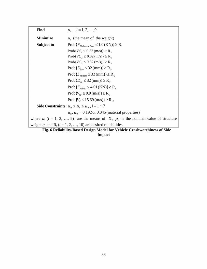
Find 9 , 2, 1,, L=iiµ

Minimize qµ (the mean of the weight) Subject to 1R(KN)} 0.1Prob{ ≥≤adAbdomen_loF 21 R(m/s)} 32.0Prob{ ≥≤VC 32 R(m/s)} 32.0Prob{ ≥≤VC 43 R(m/s)} 32.0Prob{ ≥≤VC 5R(mm)} 32Prob{ ≥≤lowD 6R(mm)} 32Prob{ ≥≤middleD 7R(mm)} 32Prob{ ≥≤upD 8R(KN)} 01.4Prob{ ≥≤PublicF 9R(m/s)} 9.9Prob{ ≥≤bpV 10R(m/s)} 69.15Prob{ ≥≤dVSide Constraints: 7~1 , =≤≤ iuiili µµµ 345.0or 192.0 , 98 =µµ (material properties)

where µi (i = 1, 2, …, 9) are the means of Xi, qµ is the nominal value of structure weight q, and Ri (i = 1, 2, …, 10) are desired reliabilities.

Fig. 6 Reliability-Based Design Model for Vehicle Crashworthiness of Side Impact

33

0 50 100 150 200 250 300 350 400 45022

23

24

25

26

27

28

29

30Convergence Histroy of the Weight

Wei

ght

Number of Function Evaluations

Opt: OptimizationRA: Reliability Assessment

Opt 1

RA1: Rmin=0.5 Opt 3 Opt 2

RA2: Rmin=0.9

RA3: Rmin=0.9

Cycle 1 Cycle 3 Cycle 2

Fig. 7 Convergence History of the Object

34

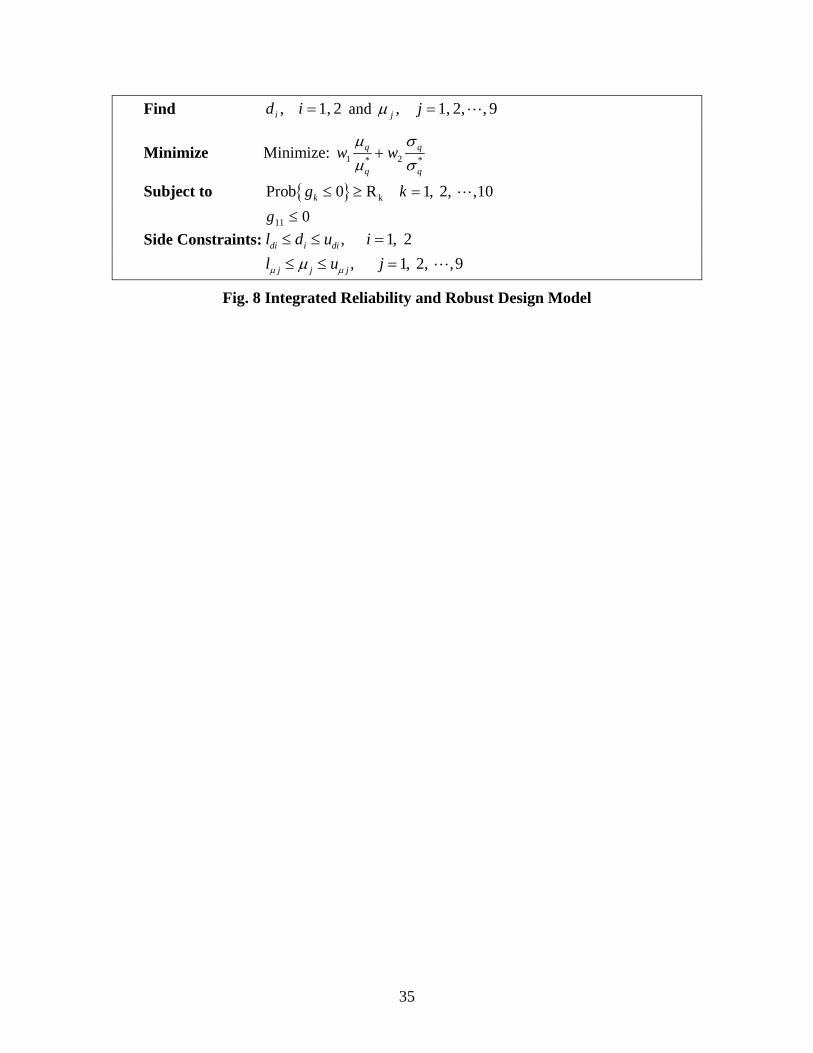
Find and 2 1,, =idi 9 , 2, 1,, L=jjµ

Minimize Minimize: 1 2* *q q

q q

w wµ σµ σ

+

Subject to { } kProb 0 R 1, 2, ,10kg k≤ ≥ = L 011 ≤gSide Constraints: , 1, 2di i dil d u i≤ ≤ = , 1, 2, ,9j j jl u jµ µµ≤ ≤ = L

Fig. 8 Integrated Reliability and Robust Design Model

35

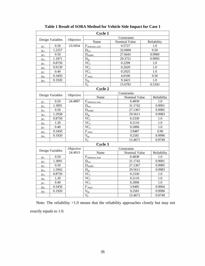
Table 1 Result of SORA Method for Vehicle Side Impact for Case 1

Cycle 1 Constraints Design Variables Objective Name Nominal Value Reliability

µ1 0.50 FAbdomen_load 0.5727 1.0 µ2 1.2257 Dlow 32.0000 0.50 µ3 0.50 Dmiddle 27.6641 0.9960 µ4 1.1871 Dup 29.3721 0.9993 µ5 0.8750 VC1 0.2299 1.0 µ6 0.9139 VC2 0.2029 1.0 µ7 0.40 VC3 0.2925 1.0 µ8 0.3450 F Pubic 4.0100 0.50 µ9 0.1920 Vbp 9.3423 1.0

23.5054

Vd 15.6781 0.5343 Cycle 2

Constraints Design Variables Objective Name Nominal Value Reliability µ1 0.50 FAbdomen_load 0.4839 1.0 µ2 1.3091 Dlow 31.1742 0.9001 µ3 0.50 Dmiddle 27.1367 0.9985 µ4 1.2938 Dup 29.5611 0.9983 µ5 0.8750 VC1 0.2330 1.0 µ6 1.20 VC2 0.2116 1.0 µ7 0.40 VC3 0.2896 1.0 µ8 0.3450 F Pubic 3.9487 0.90 µ9 0.1920 Vbp 9.2581 0.9996

24.4897

Vd 15.4671 0.9749 Cycle 3

Constraints Design Variables Name Nominal Value Reliability µ1 0.50 FAbdomen_load 0.4838 1.0 µ2 1.3091 Dlow 31.1742 0.9001 µ3 0.50 Dmiddle 27.1367 0.9985 µ4 1.2942 Dup 29.5611 0.9983 µ5 0.8750 VC1 0.2330 1.0 µ6 1.20 VC2 0.2116 1.0 µ7 0.40 VC3 0.2896 1.0 µ8 0.3450 F Pubic 3.9485 0.9004 µ9 0.1920 Vbp 9.2581 0.9996

Objective 24.4913

Vd 15.4671 0.9749

Note: The reliability =1.0 means that the reliability approaches closely but may not

exactly equals to 1.0.

36

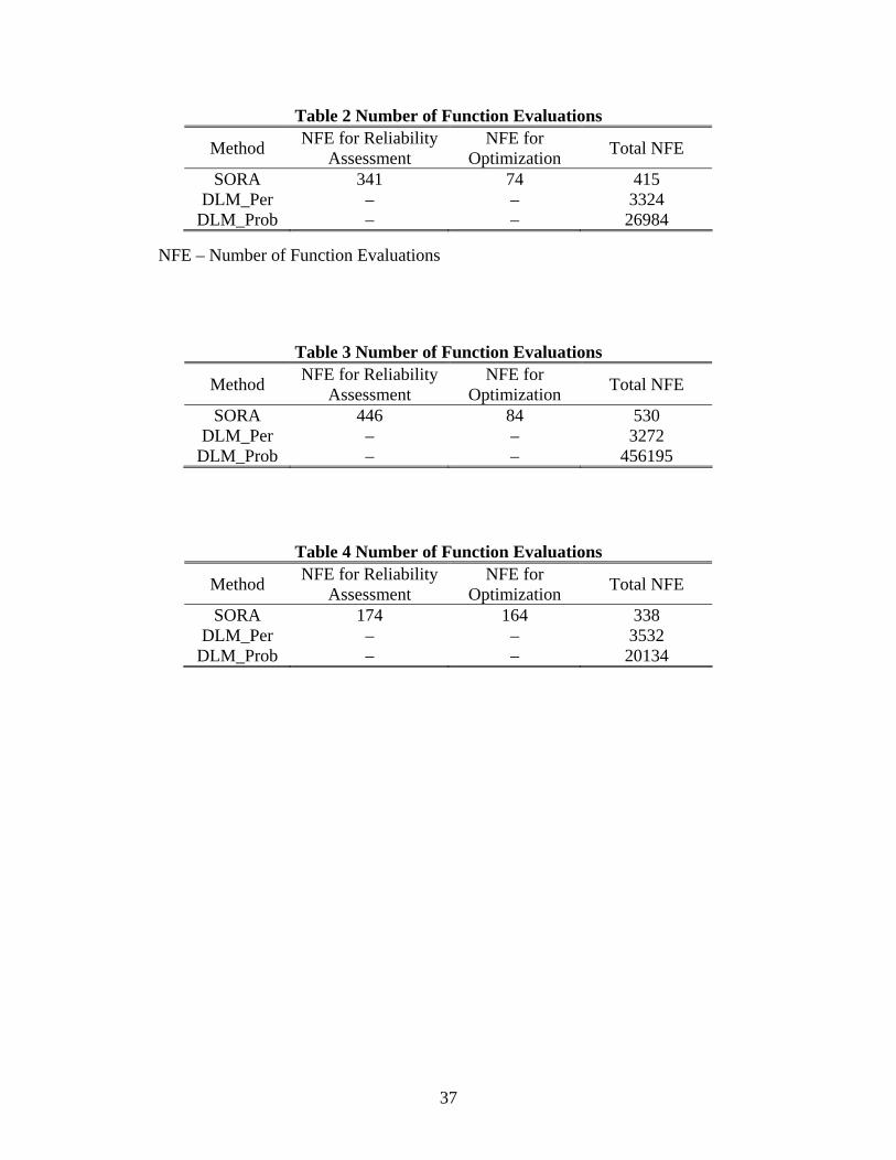
Table 2 Number of Function Evaluations

Method NFE for Reliability Assessment

NFE for Optimization Total NFE

SORA 341 74 415 DLM_Per – – 3324

DLM_Prob – – 26984

NFE – Number of Function Evaluations

Table 3 Number of Function Evaluations

Method NFE for Reliability Assessment

NFE for Optimization Total NFE

SORA 446 84 530 DLM_Per – – 3272

DLM_Prob – – 456195

Table 4 Number of Function Evaluations

Method NFE for Reliability Assessment

NFE for Optimization Total NFE

SORA 174 164 338 DLM_Per – – 3532

DLM_Prob – – 20134

37