sequences and series notes for math 3100 at the university of
TRANSCRIPT

Sequences and Series
Notes for MATH 3100
at the
University of Georgia
Spring Semester 2010
Edward A. Azoff
With additions by V. Alexeev and D. Benson


Contents
Introduction 51. Overview 52. Prerequisites 63. References 74. Notations 75. Acknowledgements 7
Chapter 1. Real Numbers 91. Fields 92. Order 123. Eventually Positive Functions 144. Absolute Value 155. Completeness 176. Induction 187. Least Upper Bounds via Decimals 21Exercises 22
Chapter 2. Sequences 271. Introduction 272. Limits 283. Algebra of Limits 324. Monotone Sequences 345. Subsequences 356. Cauchy Sequences 377. Applications of Calculus 38Exercises 39
Chapter 3. Series 451. Introduction 452. Comparison 483. Justification of Decimal Expansions 504. Ratio Test 525. Integral Test 526. Series with Sign Changes 537. Strategy 548. Abel’s Inequality and Dirichlet’s Test 55Exercises 56
3
4 CONTENTS
Chapter 4. Applications to Calculus 63Exercises 67
Chapter 5. Taylor’s Theorem 711. Statement and Proof 712. Taylor Series 753. Operations on Taylor Polynomials and Series 76Exercises 81
Chapter 6. Power Series 851. Domains of Convergence 852. Uniform Convergence 883. Analyticity of Power Series 91Exercises 92
Chapter 7. Complex Sequences and Series 951. Motivation 952. Complex Numbers 963. Complex Sequences 974. Complex Series 985. Complex Power Series 996. De Moivre’s Formula 101Exercises 102
Chapter 8. Constructions of R 1051. Formal Decimals 1062. Dedekind Cuts 1083. Cauchy Sequences 109
Index 111
Introduction
1. Overview
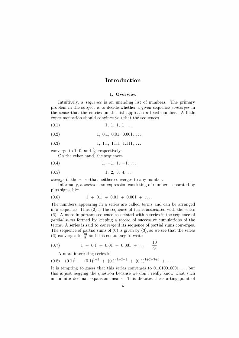
Intuitively, a sequence is an unending list of numbers. The primaryproblem in the subject is to decide whether a given sequence converges inthe sense that the entries on the list approach a fixed number. A littleexperimentation should convince you that the sequences
1, 1, 1, 1, . . .(0.1)
1, 0.1, 0.01, 0.001, . . .(0.2)
1, 1.1, 1.11, 1.111, . . .(0.3)
converge to 1, 0, and 109 respectively.
On the other hand, the sequences
1, −1, 1, −1, . . .(0.4)
1, 2, 3, 4, . . .(0.5)
diverge in the sense that neither converges to any number.Informally, a series is an expression consisting of numbers separated by
plus signs, like
1 + 0.1 + 0.01 + 0.001 + . . . .(0.6)
The numbers appearing in a series are called terms and can be arrangedin a sequence. Thus (2) is the sequence of terms associated with the series(6). A more important sequence associated with a series is the sequence ofpartial sums formed by keeping a record of successive cumulations of theterms. A series is said to converge if its sequence of partial sums converges.The sequence of partial sums of (6) is given by (3), so we see that the series(6) converges to 10
9 and it is customary to write
1 + 0.1 + 0.01 + 0.001 + . . . =10
9(0.7)
A more interesting series is
(0.1)1 + (0.1)1+2 + (0.1)1+2+3 + (0.1)1+2+3+4 + . . .(0.8)
It is tempting to guess that this series converges to 0.1010010001 . . . , butthis is just begging the question because we don’t really know what suchan infinite decimal expansion means. This dictates the starting point of
5
6 INTRODUCTION
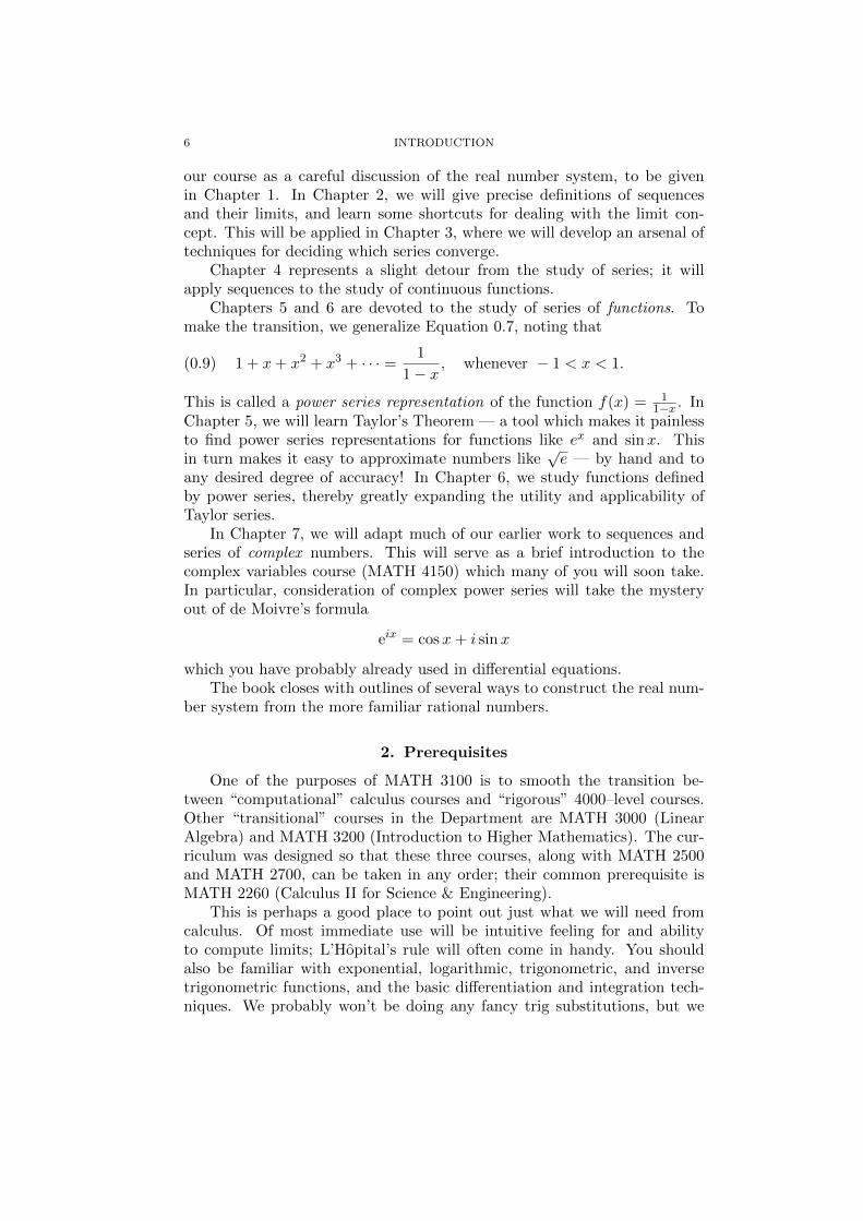
our course as a careful discussion of the real number system, to be givenin Chapter 1. In Chapter 2, we will give precise definitions of sequencesand their limits, and learn some shortcuts for dealing with the limit con-cept. This will be applied in Chapter 3, where we will develop an arsenal oftechniques for deciding which series converge.
Chapter 4 represents a slight detour from the study of series; it willapply sequences to the study of continuous functions.
Chapters 5 and 6 are devoted to the study of series of functions. Tomake the transition, we generalize Equation 0.7, noting that
1 + x+ x2 + x3 + · · · = 1
1− x, whenever − 1 < x < 1.(0.9)
This is called a power series representation of the function f(x) = 11−x . In
Chapter 5, we will learn Taylor’s Theorem — a tool which makes it painlessto find power series representations for functions like ex and sinx. Thisin turn makes it easy to approximate numbers like
√e — by hand and to
any desired degree of accuracy! In Chapter 6, we study functions definedby power series, thereby greatly expanding the utility and applicability ofTaylor series.
In Chapter 7, we will adapt much of our earlier work to sequences andseries of complex numbers. This will serve as a brief introduction to thecomplex variables course (MATH 4150) which many of you will soon take.In particular, consideration of complex power series will take the mysteryout of de Moivre’s formula
eix = cosx+ i sinx
which you have probably already used in differential equations.The book closes with outlines of several ways to construct the real num-
ber system from the more familiar rational numbers.
2. Prerequisites
One of the purposes of MATH 3100 is to smooth the transition be-tween “computational” calculus courses and “rigorous” 4000–level courses.Other “transitional” courses in the Department are MATH 3000 (LinearAlgebra) and MATH 3200 (Introduction to Higher Mathematics). The cur-riculum was designed so that these three courses, along with MATH 2500and MATH 2700, can be taken in any order; their common prerequisite isMATH 2260 (Calculus II for Science & Engineering).
This is perhaps a good place to point out just what we will need fromcalculus. Of most immediate use will be intuitive feeling for and abilityto compute limits; L’Hopital’s rule will often come in handy. You shouldalso be familiar with exponential, logarithmic, trigonometric, and inversetrigonometric functions, and the basic differentiation and integration tech-niques. We probably won’t be doing any fancy trig substitutions, but we

5. ACKNOWLEDGEMENTS 7
will definitely use the fact that∫
11+x2
dx = arctanx , and may need anoccasional partial fraction decomposition toward the end of the course.
3. References
The following sources were used in constructing notes for our course.(MATH 3100 was MAT 350 under quarters.)
(1) MAT 350 notes by Kevin F. Clancey(2) MAT 350 notes by David E. Penney(3) Calculus, by Michael Spivak, 2nd Edition, 1967, Publish or Perish,
Houston.(4) Principles of Mathematical Analysis, by Walter Rudin, 3rd Edi-
tion, 1976, McGraw Hill, New York.
Please do not hesitate to ask questions concerning these course noteseither in or out of class. Corrections and expository suggestions are alsowelcome.
4. Notations
The following are some common mathematical notations that will beused frequently when writing on the board to save time:
• ∀ for any. Example: ∀ real number x, x2 ≥ 0.• ∃ there exists. Example: ∃ a real number x with x2 < 1• x ∈ F x is an element of the set F . Example: 2 ∈ Q.• x 6∈ F x is not an element of the set F . Example:
√2 6∈ Q.
• E ⊂ F the set E is a subset of the set F , i.e. every element of Eis also an element of F : ∀x ∈ E, x ∈ F . Example: Q ⊂ R.• E 6⊂ F the set E is not a subset of the set F : ∃x ∈ F such thatx 6∈ E. Example: R 6⊂ Q.• � end of proof.
5. Acknowledgements
I would like to thank several people for contributing to the developmentof these notes. Drs. Clancey and Penney let me examine their own notesand gave me the benefit of their experience with the course. Drs. Alexeev,Benson, and Rumely provided valuable feedback on earlier versions of thenotes. In particular, Dr. Benson added the section on Dirichlet’s test, whileDr. Alexeev added the decimal-based construction of the real numbers, andtransformed my original AMSTeX file to the more flexible AMSLATeX for-mat.
I’m also grateful for numerous student suggestions over the years, es-pecially Evan Glover’s efforts to the make whole enterprise more “studentfriendly”.

8 INTRODUCTION
Section 1.3 is dedicated to the memory of David Galewski who wouldhave described it as a “sandbox” for us to play in before we get down to theserious business of defining limts.

CHAPTER 1
Real Numbers
Intuitively, real numbers are the “measure numbers”, with which onecan measure arbitrary distances. The usual model all of us have in mind isthat of a real line, with a chosen origin and unit measure. In this model,a real number corresponds to a point on the line. However, this picturerelies on properties of the physical world. What is a point on a line? Howdoes a line look when you look at it at a greater and greater magnification?Clearly, “point” and “line” are mathematical abstractions of the physicalworld, and have to be dealt with mathematically.
There are various ways to study the real number system. The “bottom-up” approach starts out with a set of axioms for the set of natural numbers{1, 2, 3, ...}, and then constructs successively larger number systems untilthe full real number system is reached. This is the approach taken in Dr.Clancey’s notes, and one you may see in MATH 4000. It makes a strong casefor the existence of the real number system, but it is somewhat technical andtakes a good deal of time to complete. We therefore postpone this discussiontill the last chapter of the book.
In this chapter, we will take the “top-down” approach: we begin bydiscussing various properties that we want the full real number system toenjoy. The goal is a minimal set of axioms which characterize the realnumber system. We then “look down” to find natural numbers, integersand rational numbers inside the reals. While not quite as advanced as thebottom–up approach, this procedure quickly sets the tone for the type ofreasoning we will be using throughout the course. Several implementationsof the “’bottom-up” approach are outlined in Chapter 8.
1. Fields
Definition 1.1. A binary operation on a set S is a function f : S×S →S. We usually write the name of the function between its arguments.
Definition 1.2. A field is a set F equipped with two binary operations,denoted “+” and · satisfying the following properties:Axioms for addition:
A1 (closure) If x ∈ F and y ∈ F , then x+ y ∈ F .A2 (commutativity) If x ∈ F and y ∈ F , then x+ y = y + x.A3 (associativity) If x, y, and z each belong to F , then (x+ y) + z =
x+ (y + z).
9
10 1. REAL NUMBERS
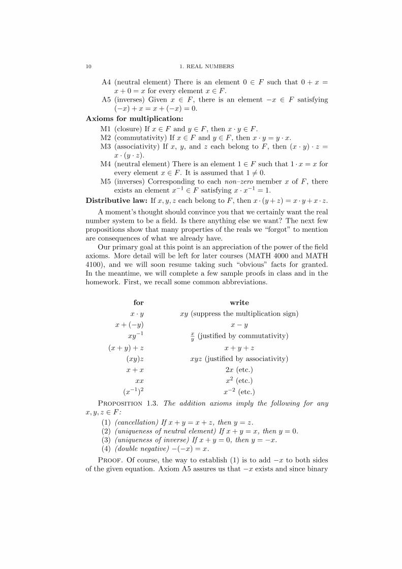
A4 (neutral element) There is an element 0 ∈ F such that 0 + x =x+ 0 = x for every element x ∈ F .
A5 (inverses) Given x ∈ F , there is an element −x ∈ F satisfying(−x) + x = x+ (−x) = 0.
Axioms for multiplication:
M1 (closure) If x ∈ F and y ∈ F , then x · y ∈ F .M2 (commutativity) If x ∈ F and y ∈ F , then x · y = y · x.M3 (associativity) If x, y, and z each belong to F , then (x · y) · z =
x · (y · z).M4 (neutral element) There is an element 1 ∈ F such that 1 ·x = x for
every element x ∈ F . It is assumed that 1 6= 0.M5 (inverses) Corresponding to each non–zero member x of F , there
exists an element x−1 ∈ F satisfying x · x−1 = 1.
Distributive law: If x, y, z each belong to F , then x · (y+ z) = x · y+x · z.A moment’s thought should convince you that we certainly want the real
number system to be a field. Is there anything else we want? The next fewpropositions show that many properties of the reals we “forgot” to mentionare consequences of what we already have.
Our primary goal at this point is an appreciation of the power of the fieldaxioms. More detail will be left for later courses (MATH 4000 and MATH4100), and we will soon resume taking such “obvious” facts for granted.In the meantime, we will complete a few sample proofs in class and in thehomework. First, we recall some common abbreviations.
for write
x · y xy (suppress the multiplication sign)
x+ (−y) x− yxy−1 x
y (justified by commutativity)
(x+ y) + z x+ y + z
(xy)z xyz (justified by associativity)
x+ x 2x (etc.)
xx x2 (etc.)
(x−1)2 x−2 (etc.)
Proposition 1.3. The addition axioms imply the following for anyx, y, z ∈ F :
(1) (cancellation) If x+ y = x+ z, then y = z.(2) (uniqueness of neutral element) If x+ y = x, then y = 0.(3) (uniqueness of inverse) If x+ y = 0, then y = −x.(4) (double negative) −(−x) = x.
Proof. Of course, the way to establish (1) is to add −x to both sidesof the given equation. Axiom A5 assures us that −x exists and since binary

1. FIELDS 11
operations are functions, we know that “equals added to equals are equal”.Thus we have
(−x) + (x+ y) = (−x) + (x+ z).(1.1)
Working on the left-hand side of this equation, we apply Axioms A5, A3, andA4 in turn to obtain (−x) + (x+ y) = ((−x) +x) + y = 0 + y = y. Similarly,the right hand side of Equation 1.1 simplifies to z, and we conclude y = zas desired.
We could repeat the preceding argument to establish (2), but it is alittle neater to apply the result of (1). Indeed, putting Axiom A4 and thehypothesis of (2) together, we have x+ y = x+ 0, and thus (1) yields y = 0as desired. The proof of (3) is similar.
Finally, for (4) write y := −x. Because y is the additive inverse of x, wehave x+ y = 0. But this equation also tells us that x is the additive inverseof y, i.e., x = −y = −(−x)as desired. �
Slight variation in the wording of this proof gives the corresponding factsfor multiplication.
Proposition 1.4. The multiplication axioms imply the following for anyx, y, z ∈ F :
(1) (cancellation) If x 6= 0 and xy = xz, then y = z.(2) (uniqueness of neutral element) If x 6= 0 and xy = x, then y = 1.(3) (uniqueness of inverse) If xy = 1, then y = x−1.(4) (double inverse) If x 6= 0 then (x−1)−1 = x.
The next result is more subtle because it simultaneously involves multi-plication and additon. This dictates the use of distributivity as that is theonly axiom involving both operations.
Proposition 1.5. The field axioms have the following consequences forany x, y ∈ F .
(1) 0x = 0.(2) xy = 0 implies x = 0 or y = 0.(3) (−x)y = −(xy) = x(−y).(4) (−x)(−y) = xy.
Proof. For (1), we apply distributivity to conclude (0 + 0)x = 0x+ 0x.Since 0 + 0 = 0, we get 0x+ 0x = 0x, whence 0x = 0 by Proposition 1.3(2).
To establish (2), we assume that xy = 0, while x 6= 0. In view of(1) and commutativity, we have xy = x0,whence y = 0 by multiplicativecancellation.
For (3), we combine distributivity and Part (1) to get (−x)y + xy =((−x) + x)y = 0y = 0, whence (−x)y must be the additive inverse of xy byProposition 1.3(3).
Applying (3) with −y playing the role of y yields(−x)(−y) = −(x(−y)) = −(−(xy)). Since this simplifies to xy by the doublenegative property, we have (4) and the proof is complete. �

12 1. REAL NUMBERS
In particular, now you finally know why (−1)(−1) = 1. Several exercisesat the end of the chapter are designed to bring home the centrality of theseobservations in school mathematics.
The following embarrassing example shows that there must be more tothe real number system than the field axioms.
Example 1.6. Take F to be the set whose only elements are 0 and 1.Define addition on F by 0 + 0 = 1 + 1 = 0 and 0 + 1 = 1 + 0 = 1. Definemultiplication on F via the equations 0(1) = 1(0) = 0(0) = 0 and 1(1) = 1.An easy but boring check shows that this F is a field.
Since there are more than two real numbers, we must be missing some-thing.
2. Order
What we need is order. It turns out to be convenient to first axiomitizethe notion of positivity.
Definition 1.7. An ordered field is a field F equipped with a distin-guished subset F+ satisfying the following.
(1) (trichotomy) If x ∈ F , then one and only one of the three state-ments x ∈ F+, x = 0, −x ∈ F+ is true.
(2) (closure) If x, y belong to F+, then x+y and xy also belong to F+.
Members of the distinguished set F+ are called positive.
The following proposition highlights the subtle power of the trichotomylaw.
Proposition 1.8. Let F be an ordered field with positive set F+.
(1) x2 ∈ F+ for each non–zero member x of F .(2) 1 ∈ F+.(3) If x ∈ F+, then x−1 also belongs to F+.
Proof. For (1), we apply the trichotomy law to x. Since x 6= 0 byhypothesis, there are really only two possibilities. If x ∈ F+, then x2 ∈ F+
by closure. On the other hand, if −x ∈ F+, then we get x2 = (−x)2 ∈ F+
by Part (4) of Proposition 1.5 and closure.Part (2) follows from Part (1) since we know that 1 = 12.For Part (3), we apply trichotomy to x−1. Having x−1 = 0 would con-
tradict Part (1) of Proposition 1.5. Having −x−1 ∈ F+ would force −1 =x(−x)−1 ∈ F+ by Part (3) of Proposition 1.5 and closure, thereby contra-dicting (2). Thus we have eliminated all possibilities except x−1 ∈ F+. �
Note that 1 + 1 must be a positive member of any ordered field, sothe field of Example 1.6 cannot be ordered. More generally, 0, 1, 1 + 1,1 + 1 + 1, etc. must be distinct in any ordered field F — intuitively Fmust contain a “copy” of the natural numbers 1, 2, 3, 4, . . . . In fact, the

2. ORDER 13
field axioms concerning inverses show that F must contain a “copy” of therational number system.
It is time to adopt the usual inequality notation associated with orderedfields. Both y > x and x < y mean y − x ∈ F+; we also write y ≥ x as anabbreviation for y > x or y = x. We say x is positive if x > 0 and we callx negative when x < 0. It is also convenient to say x is non-negative whenx ≥ 0. All the familiar rules for working with inequalities follow from whatwe’ve done so far. Once again, we practice with a few formal proofs. (Youcan now use results of Propositions 3, 4, and 5 above without comment).
Proposition 1.9. Let x, y, and z be members of an ordered field F.
(1) (unique comparability) Exactly one of the following 3 statements istrue: x < y, x = y, y < x.
(2) (transitivity) If x < y and y < z, then x < z.(3) If x < y, then x+ z < y + z.(4) If z > 0 and x < y, then xz < yz.(5) If z < 0 and x < y, then xz > yz.(6) If 0 < x < y, then y−1 < x−1.
Proof. For (1), we apply the trichotomy axiom to y − x. Indeed themutually exclusive possibilities y − x ∈ F+, y − x = 0, and −(y − x) ∈ F+
directly correspond to x < y, x = y, and x > y respectively.For (2), we apply the definition of < to conclude that both y−x and z−y
belong to F+. Thus their sum z−x must also belong to F+, and that meansthat x < z as desired. For (3), it suffices to note that (y+z)−(x+z) = y−x.
For (4), we apply the definition to get z and y − x in F+. Thus theirproduct yz − xz ∈ F+, so xz < yz as desired. The proof of (5) is similar,except that we begin by noting that −z and y − x both belong to F+.Finally, we get (6) by applying (4) with z = x−1y−1. �
The properties of Proposition 1.9 can be used to solve inequalities. Thefollowing example will be used in the next chapter.
Example 1.10. Solve the inequality 3x− 10000 > x.
Solution. Suppose first that 3x−10000 > x. Subtracting x from bothsides and dividing by 2 leads to x > 5000. So far we have only shown thatany x satisfying (*) must lie in the interval (5000,∞). Conversely, assumingx > 5000, we can multiply by 2 and add x to recover the original inequality.Thus we can say that the solution of the original inequlity is precisely theopen interval (5000,∞). �
Special care is needed when multiplying or dividing by a variable quan-tity because multiplying by a negative quantity reverses the sense of aninequality.
Example 1.11. Solve the inequality 1x > 1 (∗).
Solution. By trichotomy, there are three cases.

14 1. REAL NUMBERS
(1) x = 0 is not a solution of (*) because 10 is not even defined.
(2) When x > 0, then we can multiply both sides of (*) by x to get1 > x. Thus in order for a solution to come from this case, itmust simultaneously satisfy x > 0 and x < 1. (After checking), weconclude that the open interval (0, 1) is contained in the solutionset.
(3) When x < 0, then multiplying both sides of (*) by x reverses theinequality and we get 1 < x. Thus in order for a solution to comefrom this case, it must simultaneously satisfy x < 0 and x > 1.Since the intersection of these sets is empty, this case contributesnothing to the solution set.
Thus the solution to (*) is the interval: (0, 1). �
The main point to be made here is that uncritical multiplication of (*)by x would have given us spurrious negative solutions. We will learn moreefficient techniques for solving inequalities in Chapter 4.
3. Eventually Positive Functions
This section is dedicated to the memory of David Galewski who wouldhave described it as a “sandbox” for us to play in before we get down to theserious business of defining limts.
In later chapters, we will study various types of limits. These are state-ments concerning eventual behavior. For example, in calculus, when we
claim that the line y = 1 is a horizontal asymptote of the curve f(x) = x2−1x2+1
,
we mean that as x gets large, eventually f(x) gets and stays close to 1. Inparticular, this means that f(x) is eventually positive in the following sense.
Definition 1.12. Let f be a function mapping an ordered field F intoitself. We say f is eventually positive if there is an N ∈ F such that f(x) > 0whenever x > N .
While we haven’t finished studying it yet, you can think of F as the fieldof real numbers.
Example 1.13.
(1) The function f(x) = x2 + 1 is eventually positve since x2 + 1 > 0for all x.
(2) The function f(x) = x−100 is eventually positive since x−100 > 0whenever x > 100; in other words, the definition is satisfied bytaking N = 100.
(3) The function f(x) = x2 − 7x − 18 is eventually positive. To seethis, we write f(x) = x(x− 7)− 18 and take N = 18. Now supposex > 18. Then we have x − 7 > 1 so x(x − 7) > 18(1) = 18, andf(x) > 0 as desired.
(4) The function f(x) = 1100x
2−95x−50 is eventually positive. To see
this, write f(x) = ( 1100)[x(x− 9500)− 5000] and take N = 9501.

4. ABSOLUTE VALUE 15
(5) The function f(x) = 24−x2 is not eventually positive because f(x)is negative when x > 5.
(6) The function f(x) = sin2(πx) is not eventually positive. Eventhough f(x) is usually posiitive, it returns to zero whenever x is aninteger.
Note that we have not solved any fancy inequalities – we have onlyfound simple subsets of the full solution sets. In particular, there is nothingunique about the above choices of N . We have shown for example thatx2−7x−18 > 0 when x > 18, but the full solution set is (−∞,−2)∪ (9,∞).
It is easy to prove (and clear geometrically) not only that the functionf(x) = x2 is eventually positive, but that in fact, it eventually rises aboveand stays above any given horizontal line. This notion is captured in thefollowing definition.
Definition 1.14. We say that a function f diverges to infinity if foreach M ∈ F , it is true that the function f −M is eventually positive.
Another way of putting this is that no matter what “challenge number”M you give me, I can show that f(x) will eventually surpass it.
Example 1.15. The function f(x) = x2 − 5x diverges to infinity.
Proof. Let M > 0 be given and write f(x) −M = x2 − 5x −M =x(x − 5) −M . Take N to be the larger of 6 and M . Now suppose x > N .Then f(x) > (M)(1)−M = 0 as desired. �
We conclude this section with a different kind of proof. Rather thanshowing that a particular function is eventually positive, it provides a toolfor building new completely positive functions from old ones. The utility ofsuch results is analogous to that of the chain rule in differential calculus.
Proposition 1.16. The sum of eventually positive functions is againeventually positive.
Proof. Suppose f1 and f2 are eventually positive. Choose numbers N1
and N2 that work in the definition, i.e., we have f1(x) > 0 whenever x > N1
and f2(x) > 0 whenever x > N2. Then take N to be the maximum of N1
and N2. Now suppose x > N . Then (f + g)(x) = f(x) + g(x) > 0 + 0 = 0and we have shown that f + g satisfies the definition. �
4. Absolute Value
Absolute values will play an important role in the sequel. The intuitiveidea is that |x− y| should measure the undirected distance between x and y.
Definition 1.17. Let x be a member of an ordered field F . Then theabsolute value of x, denoted |x|, is defined by
|x| =
{x, if x ≥ 0
−x, if x < 0.
16 1. REAL NUMBERS
Example 1.18. The equation |x| = 5 has two solutions, namely x = 5and x = −5. On the other hand, the equation |x| = −2 has no solutions.
Consider next the equation 2x+ |x− 3| = 5. We deal with the absolutevalue by considering cases.
(1) x− 3 ≥ 0. Then |x− 3| = x− 3 by definition. Substituting in ourtarget equation gives 2x + (x − 3) = 5, i.e., x = 8
3 . But this is a
fake solution as it doesn’t satisfy the target equation. (Also 83 is
outside the interval defining this case.)(2) x − 3 < 0. Here the defintion yields |x − 3| = −(x − 3) = 3 − x.
Substituting in our target equation gives 2x + (3 − x) = 5, i.e.,x = 2, which does indeed satisfy the target equation.
In summary, x = 2 is the only solution of the equation 2x+ |x− 3| = 5.
Proposition 1.19. Let x and y be members of an ordered field.
(1) |xy| = |x||y|.(2) |x| is the maximum of x and −x.(3) |x| < y if and only if −y < x < y.(4) (triangle inequality) |x+ y| ≤ |x|+ |y|.
Proof. We use results of earlier propositions without comment. Thestraightforward consideration of cases needed for Part (1) is left to thereader.
For (2) we consider two cases. When x ≥ 0, we have −x ≤ 0 ≤ x,so |x| = x is indeed the maximum of x,−x. Similarly, when x < 0, then−x > 0 > x, so |x| = −x is still the maximum of x,−x.
In view of (2), the inequality |x| < y is equivalent to requiring bothx < y and −x < y. Since the latter two inequalities are in turn equivalentto the double inequality −y < x < y, we have established (3).
Applying (2) to x and y individually, we obtain
x ≤ |x|, y ≤ |y|, −x ≤ |x|, and − y ≤ |y|.Adding these in pairs gives
x+ y ≤ |x|+ |y|, and − (x+ y) ≤ |x|+ |y|.whence another appeal to Part (2) establishes (4). �
Example 1.20. By Part (3) of the preceding proposition, the inequality|x − 3| < 5 is equivalent to −5 < x − 3 < 5 and thus its solution set isthe open interval (−2, 8). Note that this corresponds to all points on thenumber line obtained by wandering at most 5 units from 3.
The solution of the opposite inequality |x−3| ≥ 5 is the complementaryset, namely the union (−∞,−2] ∪ [8,∞).
Example 1.21. How large can |x+ 6| be when |x− 3| < 1?In view of (3) of the preceding proposition, the given condition means
−1 < x − 3 < 1. Adding 9 then yields 8 < x + 6 < 10, which shows|x+ 6| < 10.

5. COMPLETENESS 17
A more sneaky approach is to use the triangle inequality to conclude|x+ 6| = |(x− 3) + 9| ≤ |x− 3|+ |9| < 10.
Example 1.22. Consider the polynomial p(x) = x2+3x. Then p(3) = 18and it seems reasonable that p(x) should be close to 18 when x is close to3. To quantify this, note that
|p(x)− 18| = |x2 + 3x− 18| = |x+ 6||x− 3|.
In view of the last example, we have
|p(x)− 18| = |x+ 6||x− 3| ≤ 10|x− 3|, whenever |x− 3| < 1.
From this it follows for example that |p(x)−18| < .01 whenever |x−3| < .001.
5. Completeness
To finish our characterization of the real number system, we must un-derstand how it differs from the rational number system. We will see shortlythat there is no rational solution to the equation x2 = 2. It’s not that wecan’t get close: the squares of 1, 1.5, 1.41, 1.414, . . . get closer and closer to2. What we need is a “limit” of these numbers; our last axiom will guaranteethat such a limit exists.
Definition 1.23. Let S be a subset of an ordered field F .
(1) An element b ∈ F is an upper bound of S if x ≤ b for all x ∈ S.(2) We call b the least upper bound of S if in addition every upper
bound a for S satisfies b ≤ a.(3) An ordered field F is said to be complete if every non-empty subset
of F which has an upper bound must have a least upper bound aswell.
It will probably take some time for you to feel comfortable with theseconcepts; that’s one of the goals of the course. As a first step, plot the setsdiscussed in the following (informal) example on a number line.
Example 1.24. Take F to be the rational numbers.
(1) If S = {x ∈ F : x < 3}, then 3, 4, and 543 are all upper bounds forS, and 3 is its least upper bound. Note that lubS /∈ S.
(2) If S = {x ∈ F : 0 < x and x2 < 2}, then 2, 1.5, 1.42, . . . are upperbounds of S, but the irrationality of
√2 means that S cannot have
a lub.(3) Take S = {.1, .101, .101001, .1010010001, . . . }. Again, there are
many upper bounds to this set, but the non–repeating nature ofthese decimal expansions rules out the existence of a rational leastupper bound for S.
No ordered field has an upper bound, much less a least upper bound. Thepoint of the preceding example is that some bounded sets of rational num-bers have least upper bounds and others don’t. This means that the rational

18 1. REAL NUMBERS
number field is not complete. Geometrically, not all points on a line can beaccounted for by plotting rational distances.
There are several competing notions of completeness in mathematics,but in this course “complete” will always be used in the sense of Definition1.23. Hopefully, you are convinced that the real number system should bea complete ordered field, but several questions remain.
(1) How do we know that there are any complete ordered fields?(2) How different can two complete ordered fields be?(3) Have we left anything out in our characterization of the real number
system?
Question 1 is addressed by constructing the reals from more primitivesystems. We will return to this topic in Chapter 8, to which you can skipahead now if your curiosity has gotten the best of you.
As for Question 2, we could obviously call numbers by different names -their French names for example - but the resulting number system wouldreally be the same. Thus you don’t have to learn a new set of “tables” to doarithmetic in French: to compute deux fois quatre, you could first translateto the English problem two times four, next do the computation in English toget eight, and finally translate the answer back to get the French huit. Thesecond part of the following theorem states that any two complete orderedfields are related in this way. Think of the function f (technically known asan isomorphism) as a dictionary.
Theorem 1.25. (without proof)
(1) Complete ordered fields exist.(2) Suppose both R and R′ are both complete ordered fields. Then there
is a one-to-one, onto function f : R→ R′ which respects all orderedfield structures, e.g., f(x+ y) = f(x) +′ f(y) for all x, y ∈ R; here+ denotes addition in R , while +′ denotes addition in R′.
Definition 1.26. The real number system is a fixed complete orderedfield. It is denoted R.
The essential uniqueness of the real number system is also reassuringconcerning Question 3 - we have successfully characterized the system.
6. Induction
Our next task is to identify the natural, integral, and rational numbersystems as subsets of R (the “down” part of our top–down approach).
Definition 1.27.
(1) A subset S of R is inductive if x+ 1 ∈ S whenever x ∈ S.(2) The set of natural numbers is the intersection of all inductive sub-
sets of R which contain 1. It is denoted N.(3) The set of integers, denoted Z , is defined by Z = {x ∈ R : x = m−n
for some m,n ∈ N}.

6. INDUCTION 19
(4) The set of rational numbers , denoted Q , is defined by Q = {x ∈R : x = m
n for some m,n ∈ Z with n 6= 0}.
The interval [1,∞) = {x ∈ R|x ≥ 1} is an inductive set containing1. Since N is the intersection of all such sets, we see that N ⊂ [1,∞). Inparticular, every natural number is positive and 1 is the smallest memberof N. A more subtle inductive set is {x ∈ R|x = 1 or x ≥ 1 + 1}. Since Nmust be contained in this set as well, we see that there is no natural numberbetween 1 and 2.
It is an exercise to show that N is an inductive set. Since 1 ∈ N , it followsthat 1 + 1 = 2 ∈ N, whence 3 ∈ N , etc; since N is the smallest inductivesubset of R, we see that we really have captured the natural number system.The next Proposition shows that the principle of mathematical induction isbuilt into the definition of N.
Proposition 1.28. (Principle of Mathematical Induction) Suppose S isan inductive subset of N containing 1. Then S = N.
Proof. We have S ⊂ N by hypothesis. The opposite inclusion N ⊂ Sfollows since N is the intersection of all inductive sets containing 1. �
The Principle of Mathematical Induction will play an important role inour course. The following two applications are typical.
Example 1.29. Use induction to prove that 1+3+5+· · ·+(2n−1) = n2
for every natural number n.
Solution. Set S = {n ∈ N : 1 + 3 + 5 + · · ·+ (2n− 1) = n2}. Note firstthat 1 ∈ S since 1 = 12.
To see that S is inductive, suppose that k ∈ S. Then 1 + 3 + 5 + · · ·+(2k − 1) = k2. Adding 2[k + 1]− 1 to both sides of this equation yields
1 + 3 + 5 + · · ·+ (2k − 1) + (2[k + 1]− 1) = k2 + 2k + 1 = (k + 1)2
which means that k + 1 ∈ S. This completes the proof that S is inductive.The Principle of Mathematical Induction ( Proposition 1.28) allows us
to conclude that S = N and thus completes the proof. �
You can use the abbreviation “by induction” for “by the Principle ofMathematical Induction”.
Example 1.30. Let a > 1 Use induction to prove that an > 1 for everynatural number n.
Solution. Set S = {n ∈ N : an > 1}. Note first that 1 ∈ S since a1 = a.To see that S is inductive, suppose that k ∈ S. Then ak > 1. Multiplying
both sides of this inequality by the positive number a yields ak+1 > a. Bytransitivity of inequality, we have ak+1 > a > 1 which means that k+1 ∈ S.By induction, we conclude that S = N and the proof is complete. �
20 1. REAL NUMBERS
There are sevral variations of mathematical induction. These are logi-cally equivalent to one another, but there are times when one is more con-venient than others. The proofs of the following versions are deferred to theexercises.
Proposition 1.31 (Well-Ordering Principle). Every non-empty subsetof N has a smallest member.
Proposition 1.32 (Strong Induction). Suppose S is a set of naturalnumbers satisfying the following:
(1) 1 ∈ S.(2) For each natural number n, if all of the natural numbers which are
less than or equal to n belong to S, then n+ 1 belongs to S as well.
Then S = N.
The difference between this and regular induction is in (2) where we getto assume n and all natural numbers below it belong to S.
A natural number is prime if it has exaclty two positive integral divi-sorss, namely 1 and itself. The first few primes are 2, 3, 5 . . . . An integergreater than 1 which is not prime is said to be composite. Note that by thisconvention, the integer 1 is neither prime nor composite.
Corollary 1.33. Every composite natural number has a prime divisor.
Proof. Set S := {n ∈ N|n = 1 or n has a prime factor.}. Since 1 ∈S is given, we only need to establish the implication 1.32(2). So assume1, 2, . . . n all belong to S. We must show that n+1 ∈ S. Since every numberis a divisor of itself, this is clear when n+ 1 is prime. On the other hand, ifn + 1 is composite, then it must have a divisor x satisfying 1 < x < n + 1.But then our inductive hypothesis assures us that x has a prime factor p.But that would make p a prime factor of n+ 1 as well, so n+ 1 ∈ S in anycase. We conclude that S = N and the proof is complete. �
The discussion in the following example is somewhat naive. Full justifi-cation can be found in Section 1-8 of Topology, by James R. Munkres, 1975,Prentice-Hall, Engelwoods, N.J.
Example 1.34. Induction can be used to define functions on the naturalnumbers. (This procedure is also known as recursion). To illustrate withfactorials, set 1! = 1 and (n+ 1)! = (n+ 1)n!. The set S of natural numberswhose factorials are defined by this prescription includes 1 and is inductive.It follows from Proposition 1.28 that the factorials of all natural numbersare thus defined. Use of this procedure to compute 5! helps explain whyinduction is the mathematical version of the “domino theory”.
We proceed to our first application of completeness of R. Proposition1.35 will be used frequently in the sequel.
Proposition 1.35. The set N of natural numbers does not have an upperbound.

7. LEAST UPPER BOUNDS VIA DECIMALS 21
Proof. We argue by contradiction. If N had an upper bound, it wouldhave a least upper bound b. But then b − 1 could not be an upper boundof N, so there would be a natural number n > b − 1. This however impliesthat n + 1 > b, contradicting the fact that b was supposed to be an upperbound of N. �
Corollary 1.36. (Archimedean Principle) Suppose x and y are positivereal numbers. Then there is a natural number n satisfying nx > y.
Proof. The preceding proposition provides a natural number n > yx .�
There is a folk version of the Archimedean Principle: “every little bithelps”. No matter how small x is, if you keep progressing by that amount,there is no limit on how high you can go.
We continue with the promised proof that√
2 cannot be rational. Theargument illustrates the more informal approach to the real numbers whichwill be taken in later chapters. Field properties are used without comment.More significantly, the possibility of reducing fractions to lowest terms istaken for granted, even though we have not shown how this follows fromCorollary 1.33. (See Problem 1.63).
Proposition 1.37. The equation x2 = 2 does not have a rational solu-tion.
Proof. We argue by contradiction, assuming that x2 = 2 for some ra-tional x. By definition of rational, we may write x = p
q for some integers
p, q. We may assume that this fraction is in lowest terms. Algebraic ma-nipulations lead to the equation 2q2 = p2. This implies that p2 is even, sop must be even too. Thus we can write p = 2k for some integer k, whencesubstitution and cancellation yield q2 = 2k2. This however means that q iseven too, and contradicts the assumption that the fraction p
q was in lowest
terms. �
7. Least Upper Bounds via Decimals
Prior to coming to this course, you probably thought of real numbersas (possibly nonterminating) decimals. The steps to making this preciseinclude
(1) interpreting decimals as infinite series(2) proving that the series of (1) always converge(3) proving there is a one-to-one correspondence between real numbers
and decimals which do not end in all 9’s (we temporarily call thelatter standard).
(4) describing how decimal expansions can be used to determine whenone real number is smaller than another
We will carry out this program in Chapter 3. In Section 8.1 (which canbe read now), we will even see that this point of view can be turned around,

22 1. REAL NUMBERS
i.e., introducing decimals in a purely formal way provides one method ofconstructing the complete ordered field guaranteed by Theorem 1.14.1.
At this point, we only want to use decimals to bolster our intuitionconcerning order completeness. To do so, we take Items 1–4 for granted.The order promised by (4) is lexicographic, e.g., if x = .x1x2x3 . . . andy = .y1y2y3 . . . are standard decimal expansions, then x < y if and onlyif these expansions are not identical, and xi < yi at their first point ofdisagreement.
Now suppose that S is a non-empty subset of the open interval (0, 1) :={x ∈ R : 0 < x < 1}. Since S is bounded, it should have a least upper boundb. In fact, we can “construct” b. Take b1 to be the largest integer appearingas the first digit in the standard expansion of some member of S. Next takeb2 to be the largest integer appearing as the second standard digit of somemember of S whose first standard digit is b1. Continue inductively, takingbn+1 to be largest integer appearing as the (n + 1)’st standard digit in theexpansion of
{x ∈ S : the standard expansion of x begins with .b1 . . . bn }.
Then b = .b1b2b3 . . . may end in all 9’s, but in any case it will represent theleast upper bound of S.
Exercises
Unless otherwise stated, a, b, c, d, and x stand for real numbers through-out these exercises.
Field Axioms
Problem 1.1. Prove Part (3) of Proposition 1.3. You can either mimickthe proof of Part (2) or base your argument on the equation c = (b+a)+c =b+ (a+ c) = b .
Problem 1.2. Which addiiion axion is not used in the proofs of Propo-sition 1.3?
Problem 1.3. Prove Proposition 1.4.
Problem 1.4. Give examples to show that the hypothesis x 6= 0 cannotbe omitted from Parts (1), (2) and (4) of Proposition 1.4. Why wasn’t thishypothesis included in (3) ?
Problem 1.5. Give another proof of the fact that 0x = 0 by applyingdistributivity to the expression (0 + 1)x.
Problem 1.6. Prove that (a+ b)(a− b) = a2 − b2.
Problem 1.7. (Suggested by Brandon Samples) Suppose a set F isequipped with two binary operations satisfying all the field axioms exceptthat 0 = 1. Show that F has only one element.

EXERCISES 23
Problem 1.8. Construct a field with exactly three elements : 0, 1, andα. You need not verify all the axioms, but you should exhibit the additionand multiplication tables.
Problem 1.9. Suppose a 6= 0 and b 6= 0. Explain why ab 6= 0.
Problem 1.10. Write up a solution of the equation 3x + 5 = 7 for amiddle school algebra class. Then write a one or two paragraph discussionof the role of the basic field axioms and properties in your solution.
Problem 1.11. Criticize and correct the following solution of the equa-tion x2 = 6x.
“Dividing by x, we obtain x = 6, which is thus the unique solution.”
Problem 1.12. Write up a solution of the equation x2−4x−21 = 0 fora middle school algebra class which hasn’t yet been learned the quadraticformula. Then write a one or two paragraph discussion of the role of thebasic field axioms and properties in your solution.
Problem 1.13. Criticize and correct the following solution of the equa-tion x+
√x = 6.
“Transposing x and squaring both sides of the equation, we obtain x =36−12x+x2. From here, we tanspose and factor to obtain (x−4)(x−9) = 0.Thus the orgininal equation has two solutions, x = 4 and x = 9.”
Problem 1.14. While it is always desirable to check solutions to equa-tions, sometimes it is essential. Explain the relevance of the last four prob-lems to this assertion.
Problem 1.15. Prove that if neither b nor c is zero, then ab = ac
bc . Hint:Compute the product of each side of the equation with bc and compare.
Problem 1.16. Suppose bd 6= 0. Prove that ab + c
d = ad+bcbd .
Order
Problem 1.17. Prove Parts (3) and (5) of Proposition 1.9.
Problem 1.18. Prove that if a > b > 0 then a2 > b2.
Problem 1.19. Suppose a > 0, b > 0, and a2 > b2. Prove that a > b.
Problem 1.20. Prove that if x and y are both negative, then theirproduct xy is positive. Then explain why this does not contradict the closureassertion in Definition 1.7.
Problem 1.21. Write up a solution of the inequality 2 − 5x < 9 for amiddle school algebra class. Then write a one or two paragraph discussionof the role of the basic order axioms and properties in your solution.
Problem 1.22. Find all solutions of the equation |2x|+ |x− 3| = 5.
Problem 1.23. Prove Proposition 1.19.1.
24 1. REAL NUMBERS
Problem 1.24. Let a, b, c be members of an ordered field. Define whatis meant by the maximum of a, b, denoted max(a, b). Then show thatmax(a, b) ≤ c if and only if a ≤ c and b ≤ c both hold. This is used inthe proof of Proposition 1.19.2.
Problem 1.25. Prove that |a| ≤ b if and only if −b ≤ a ≤ b.
Problem 1.26. Solve each of the following four inequalities:|x| < 3, |x| < −3, |x| > 3, and |x| > −3, expressing your answers interms of intervals of real numbers.
Problem 1.27. Graph the solution of the inequality |x − 2| < 4 on anumber line.
Problem 1.28. Apply the triangle inequality to |a| = |(a − b) + b| toshow that |a| − |b| ≤ |a− b| for all a, b ∈ R. Then use symmetry to concludethat ||a| − |b|| ≤ |a− b| for all a, b ∈ R.
Problem 1.29. Suppose |x− 5| < 1. Prove the following:
(1) |x+ 8| < 14(2) |x2 + 3x− 40| ≤ 14|x− 5|(3) If |x− 5| < .001, then |x2 + 3x− 40| < .014
Problem 1.30. Prove that if |x− 110 | <
120 , then |x| > 1
20 .
Problem 1.31. Prove that if |x− 2| < 0.001 then |x2 − 4| < 0.005.
Problem 1.32. The next to the last line of Example 1.22 reads
|p(x)− 18| = |x+ 6||x− 3| ≤ 10|x− 3|, whenever |x− 3| < 1.
. Why can’t the symbol “≤ be replaced by strict inequality?
Eventual Positivity
Problem 1.33. Show that the following polynomials are eventually pos-itive.
(1) x2 + 15x(2) x2 − 15x(3) x2 + 15x− 38(4) x3 + 5x2 − 11x− 43
Problem 1.34. Prove that the product of any two eventually positivefunctions is again eventually positive.
Problem 1.35. Give an example of two functions f, g, neither of whichis eventually positive, but whose product fg is eventually positive.
Problem 1.36. Give an example of two functions f, g, neither of whichis eventually positive, but whose sum f + g is eventually positive.
Problem 1.37. In the proof of Example 1.15, why is it assumed thatM > 0 ?
EXERCISES 25
Problem 1.38. Prove that if a and b are any real numbers, then thefunction f(x) = x2 + ax+ b is eventually positive.
Problem 1.39. Give an example of a strictly increasing function whichis eventually positive, but does not diverge to infinity.
Problem 1.40. Prove that if two functions both diverge to infinity, thentheir sum also diverges to infinity.
Completeness
Problem 1.41. Suppose that b and c are both least upper bounds of asubset S of R. Prove that b = c.
Problem 1.42. Suppose b is an upper bound of a set S of real numbers.Prove that b is the least upper bound of S if and only if for each ε > 0 ,there exists an a ∈ S with a > b− ε.
Problem 1.43. Define lower bound and greatest lower bound. Thenprove that every non-empty subset S of R which has a lower bound musthave a greatest lower bound. Hint : Consider the set T = {−a : a ∈ S}.
Problem 1.44. Give an example of a set of real numbers which has anupper bound but does not have a lower bound.
Problem 1.45. Take S = {a ∈ R : 0 < a and a2 < 3}. Find severalupper bounds for S and then find its least upper bound.
Problem 1.46. Find the greatest lower bound and least upper boundof the set { 1n : n ∈ N}.
Problem 1.47. Find the greatest lower bound and least upper boundof {n−1n : n ∈ N}.
Problem 1.48. Let F be an ordered field. Prove that F+ does not havea least upper bound. Explain why this doesn’t contradict Theorem 1.25.1.
Problem 1.49. Detail the meaning of the phrase “respects all of theordered field structures” appearing in the statement of Theorem 1.25.2.
Induction
Problem 1.50. Describe four different inductive subsets of R.
Problem 1.51. How many bounded inductive subsets of R are there?
Problem 1.52. Prove that N is an inductive set.
Problem 1.53. Use induction to prove that 1 + 2 + · · ·+n = n(n+1)2 for
every natural number n.
Problem 1.54. Use induction to prove that 1 + 2 + · · ·+ 2n−1 = 2n− 1for every natural number n.

26 1. REAL NUMBERS
Problem 1.55. Use induction to prove that if 0 < a < 1 then 0 < an < 1for every natural number n. What can you say if we only assume a < 1, butnot that a > 0?
Problem 1.56. Use induction to prove that if |a| < 1 then |an| < 1 forevery natural number n.
Problem 1.57. Argue inductively on degree to prove that everynon-constant monic polynomial is eventually positive.
Problem 1.58. Argue inductively on degree to prove that every non-constant monic polynomial diverges to infinity.
Problem 1.59. Use the inductive definition of Example 1.34 to compute5!.
Problem 1.60. Use Example 1.34 to explain why it is reasonable todefine 0! = 1.
Problem 1.61. Use induction to prove that every natural number n isgreater than or equal to one, and hence positive.
Problem 1.62. Prove that for each natural number n, either n = 1 orn− 1 is also a natural number.
Problem 1.63. Use the result of the last problem to prove the wellordering principle, Proposition 1.31. Hint: assume that S does not have asmallest member and apply regular induction to show that the complementof S in N would have to exhaust N.
Problem 1.64. How does the result of the last Problem compare withthe result of Problem 1.43 ?
Problem 1.65. Use the well-ordering principle 1.31 to prove the stronginduction principle 1.32.
Problem 1.66. Is N a field? How about Z? How about Q? No proofsare required, but detail which field axioms hold in each case.
Problem 1.67. Prove that there is a rational number between any tworeals.
Decimals
Problem 1.68. Apply the technique of Section 1.5 to find decimal ex-pansions for the least upper bounds of the following sets:
(1) {1225 ,12 ,
9100}
(2) {x ∈ R+ : x ≤ 12}
(3) {x ∈ R+ : x < 12}
(4) { 37100 − 10−n : n ∈ N}
CHAPTER 2
Sequences
1. Introduction
Definition 2.1. A sequence of real numbers is a function mapping Ninto R.
You are probably accustomed to using letters like f or g to denote func-tions and x or t for their independent variables. In studying sequences, it istraditional to employ letters k, l,m, n for natural numbers and letters nearthe beginning of the alphabet for the names of the functions themselves.This should not cause any particular problem. If a is a sequence, it is con-ventional to write an in place of a(n); in prose, this is referred to as then’th term of the sequence. We will also write (an)∞n=1 or even (an) for thefunction a. The use of parentheses instead of the more traditional bracesemphasizes the distinction between functions and their ranges. For example,the sequences ((−1)n) and
((−1)n+1
)are different even though they share
the range {−1, 1}. It should also be kept in mind, here and in the sequel,that ∞ does not stand for any real number, but is used as a mnemonicdevice for an ongoing process.
The usual way to present a sequence is to give a formula for its generalterm. This was done implicitly in the preceding paragraph. A less precisebut often suggestive method is to list the few terms of a sequence, leavingit to the reader to find “the” formula for the general term.
Example 1.34 illustrated the fact that sequences can also be definedinductively (also called recursively). The next example reviews Newton’smethod, an important instance of this procedure you may have seen incalculus.
Example 2.2. Fix a real–valued function f defined on some domainD ⊂ R. Start with any a1 ∈ D. Assuming an has been defined, take an+1
to be the x–coordinate of the point where the line tangent to the graph off at (a, f(a)) intersects the x-axis. The explicit formula is
(2.1) an+1 = an −f(an)
f ′(an).
The following special case of Example 2.2 will be used to illustrate severalconcepts in this chapter.
27
28 2. SEQUENCES
Example 2.3. Apply Newton’s method with f(x) = x2 − 2 and a1 = 2.The inductive formula can be written as
(2.2) an+1 =an2
+1
anfor n ∈ N.
2. Limits
In Chapter 1, we introduced the concepts of eventual positivity anddivergence to infinity. These are easily adapted to sequences.
Definition 2.4. A sequence (an) is eventually positive if there is a nat-ural number N such that an > 0 whenever n > N .
Definition 2.5. A sequence (an) diverges to infinity if for each numberM it is true that the sequence (an −M) is eventually positive.
It is important to understand that the second definition provides a pre-cise way of saying that the terms of the sequence eventually pass and staypast each “challenge number” M .
We now want to capture the notion of what it means for the terms in asequence (an) to approach a fixed number L.
Example 2.6. Consider the sequence given by an = 3n3n−10000 . The first
few terms are close to zero, e.g. a1 = −39997 , a2 = −6
9994 . Looking ahead abit though, it seems that the numerator might overwhelm the denominator,e.g., a3332 = −2499, a3333 = −9999. Taking a really long term view however,we see that eventually the 10000 in the denominator becomes less relevantand an looks like 3n
3n = 1, e.g., a10000 = 3000020000 = 1.5, a20000 = 60000
50000 =
1.2, a1000000 = 30000002990000 ≈ 1.003. The convergence concept is only concerned
with the long-term view, so this sequence should converge to 1.
We now formulate the precise definition. In a nutshell, instead of claim-ing that an is eventually large as we did in Definition 2.5, we now want toguarantee that an is eventually “close to” L. The difference between twonumbers measures how close they are; since we don’t really care which islarger, it is more appropriate to use the absolute value of the difference.This leads to the pseudo-definition “When n is large, |an−L| is small”. Buthow small is “small” ? We take our cue from Defintion 2.5 where we de-manded that the sequence eventually meet every largeness test. Similarly,the following definition demands that the sequence eventually meet everycloseness test.
Definition 2.7. The sequence (an) is said to converge to the number Lif for each number ε > 0 there is a natural number N such that |an−L| < εwhenever n ≥ N .
The logical structure here is subtle: your give me the closeness challenge“make |an − L| < ε” and I meet it by showing you that it will “eventually”(n ≥ N) happen. Our first few examples involve minimal algebra.

2. LIMITS 29
Proposition 2.8. For any real number c, the constant sequence (c)∞n=1converges to c.
Proof. In the notation of Definition 2.7, our sequence is defined byan = c for each n and L = c as well. Let ε > 0 be given. Take N = 1 (AnyN would do). Now suppose n ≥ N . Then |an − L| = |c − c| = 0 < ε asdesired. �
Example 2.9. Show that the sequence given by an =
{n, n < 100,
5, n ≥ 100converges to 5.
Proof. Given ε > 0, take N = 100. Then whenever n ≥ N , it followsthat |an − L| = |5− 5| = 0 < ε as desired. �
Proposition 2.10. The sequence(1n
)∞n=1
converges to 0.
Proof. Let ε > 0 be given.[This paragraph is not part of the formal proof, but it illustrates how
one thinks ahead to find N . We want to guarantee | 1n − 0| < ε. But since nis to be a positive integer, the absolute value is redundent. Thus we reallywant 1
n < ε, which is equivalent to n > 1ε .]
Returning to the formal proof, apply the Archimedean Principle 1.35 toget a natural number N > 1
ε . Then n ≥ N forces the desired inequality∣∣∣∣ 1n − 0
∣∣∣∣ =1
n≤ 1
N< ε.
�
Definition 2.11. A sequence which does not converge to any real num-ber is said to diverge. If (an) does converge to L, we also say that L is thelimit of the sequence and write limn→∞ an = L.
As expected, any sequence like (√n) which diverges to infinity will di-
verge in the sense of 2.11 as well. But there are other ways for a sequenceto diverge. For example, ((−1)n) diverges because its terms jump back andforth between 1 and −1, and thus never approach a fixed limit.
On the other hand, having the signs of the terms of a sequence alternatedoes not automatically preclude convergence.
Example 2.12. The sequence(100(−1)n
n
)converges to 0.
Proof. For every n we have,
(2.3) |an − 0| =∣∣∣∣100(−1)n
n
∣∣∣∣ =100
n,
and we can argue as in Proposition 2.10. Indeed, given ε > 0, choose anatural number N > 100
ε . Then assuming n ≥ N , we can continue the

30 2. SEQUENCES
preceding display as
|an − 0| =∣∣∣∣100(−1)n
n
∣∣∣∣ =100
n≤ 100
N< ε.
�
In more algebraically complicated examples, one should concentrate onthe target quantity |an−L|, applying the triangle inequality when possible.
Example 2.13. Show that limn→∞2n2+3nn2+5
= 2
Outline. Begin by working on the target quantity:
(2.4)
∣∣∣∣2n2 + 3n
n2 + 5− 2
∣∣∣∣ =|3n− 10|n2 + 5
≤ |3n− 10|n2
≤ 3n
n2+
10
n2≤ 13
n
Once you justify each step in this computation, you can introduce ε andcontinue as in the last proof. �
Here is a formal proof of the conclusion of Example 2.6. A little morealgebraic creativity is called for because the sign in the denominator is notso cooperative.
Example 2.14. Show that limn→∞3n
3n−10000 = 1
Proof. We begin by noting that 3n− 10000 > n when n > 5000. Thuswe have
(2.5)
∣∣∣∣ 3n
3n− 10000− 1
∣∣∣∣ =
∣∣∣∣ 10000
3n− 10000
∣∣∣∣ < 10000
n, whenever n > 5000.
Given ε > 0, we choose N to be an integer larger than the maximum of 5000and 10000
ε . The reason for involving 5000 is to make Inequality 2.5 applicable.Indeed, when n ≥ N , we can continue the preceding computation to get thedesired inequality:∣∣∣∣ 3n
3n− 10000− 1
∣∣∣∣ < 10000
n≤ 10000
N< ε.
�
We conclude this section by exploiting the analogy between definitions2.5 and 2.7 to develop a more systematic appproach to the preceding proofs.While this development will in turn be superceded in the next section, itprovides a good opportunity to gain insight on the limit concept.
We write limn→∞ an = ∞ when the sequence (an) diverges to ∞. Forconvenience, we also allow the first few terms of a sequence to be undefined.
The observation that reciprocals of large numbers are small provides auseful generalization of Proposition 2.10.
Proposition 2.15. If limn→∞ an =∞ then limn→∞1an
= 0
2. LIMITS 31
Proof. Let ε > 0 be given. By definition of “diverges to infinity”,we can find a real number N so that an > 1
ε whenever n > N . By theArchimedean prinicple, we can even assume N ∈ N. Now suppose n > N .Then an >
1ε implies | 1an − 0| = 1
an< ε as desired. �
Next we solve an exercise from the last chapter.
Proposition 2.16. Let p be a non-constant monic polynomial. Thenlimn→∞ p(n) =∞.
Proof. We argue inductively on the degree of p. Suppose first that phas degree one. Thus p(x) = x + a for some a ∈ R. Now let a challengenumber M ∈ R be given and take N to be a natural number greater thanM − a.. Suppose n > N . Then an = n + a > M − a + a = M . Thisestablishes the desired result for all monic polynomials of degree one.
For the inductive step, assume the desired result holds for polynomialsof degree k and let p be a monic polynomial of degree k+1. By isolating theconstant term and factoring x out of the rest, we can write p(x) = xq(x)+afor some monic polynomial q and constant a. Let a challenge number M > 0be given. Since q has degree k, the inductive hypothesis provides a naturalnumber N such that q(n) > M + |a| whenever n > N . But then n > Nimplies p(n) = nq(n) + a ≥ q(n) + a > M + |a|+ a ≥M , and the inductivestep is established.
An appeal to PMI completes the proof. �
Corollary 2.17. Let p and q be polynomials with q having larger degree
than p. Then limn→∞p(n)q(n) = 0.
Proof. Dividing both p and q by the leading coefficient of q if necessary,we may as well asume q is monic. Let ε > 0 be given. By hypothesis, allthree polynomials q, q − p
ε , and q + pε are monic. Thus they all diverge to
∞ and in particular are eventually positive. Choose N ∈ N so that n > Nimplies
q(n)− p(n)
ε> 0 and q(n) +
p(n)
ε> 0.
Algebraic manipulation then tells us that −ε < p(n)
q(n)< ε whenever
n ≥ N , completing the proof. �
Corollary 2.18. Suppose p and q are polynomials of equal degree and
write L for the quotient of their leading coefficients. Then limn→∞p(n)q(n) = L.
Proof. Set r(x) = p(x)− Lq(x). Then for each n we have∣∣∣∣p(n)
q(n)− L
∣∣∣∣ =
∣∣∣∣r(n)
q(n)
∣∣∣∣ .Since the degree of q exceeds the degree of r, an appeal to previous corollarycompletes the proof. �
32 2. SEQUENCES
Note that all the examples in this section are special cases of the lasttwo corollaries.
3. Algebra of Limits
In calculus, you learned the definition of derivative and were probablyforced to evaluate a few derivatives directly from the definition. This wasnecessary to understand the concept, but more efficient computational tools
are needed to differentiate functions like esin x
x2+1. The situation is analogous for
convergence of sequences. While Examples 2.10ff and the related exerciseswere “for your own good”, the time has come to develop better computa-tional tools.
Proposition 2.19. Suppose the sequence (an) converges to to a realnumber L > 0. Then there is a natural number N such that an > 0 for alln ≥ N .
Proof. The difference between this situation and those in the precedingsection is that we are given the existence of a limit. Thus we don’t have toshow that something is true for every ε > 0; we know and can use that fact.Moreover, there’s no requirement to use every ε; we can choose which one(s)we find conveneint.
So take ε = L. By definition of convergence, there is a natural numberN such that n ≥ N implies |an − L| < ε. The latter inequality implies−L < an − L which in turn implies an > 0. �
Definition 2.20. A sequence (an) is
bounded above if the set {an : n ∈ N} has an upper bound;bounded below if the set {an : n ∈ N} has an lower bound;
bounded if it is simultaneously bounded above and below.
Proposition 2.21. Every convergent sequence is bounded.
Proof. Suppose (an) converges to L. Taking ε = 1 (any fixed ε woulddo), we find a natural number N such that n ≥ N implies |an − L| < 1.This means −1 < an − L < 1. Thus L − 1 < an < L + 1 for all n ≥ N . Itfollows that max{a1, a2, . . . , aN−1, L + 1} provides an upper bound for thesequence. A similar expression provides a lower bound for the sequence. �
As real-valued functions, sequences can be added, subtracted, and mul-tiplied. Division can present a problem since we can’t divide by zero. Inorder to minimize the inconvenience, we agree to broaden the definition ofsequence to allow functions whose domains take the form {n ∈ N : n ≥ N}for some fixed natural number N .
Example 2.22. For each natural number n take an = 1, bn = n−2, andcn = sin nπ
2 . We consider ab to be a sequence with domain {n ∈ N : n ≥ 3};
the usual notations for this sequence are(
1n−2
)∞n=3
and(
1n−2
)n≥3
. On the

3. ALGEBRA OF LIMITS 33
other hand, since cn = 0 for all even n, we do not consider ac as a sequence
at all.
Proposition 2.23. Suppose lim an = L.
(1) limKan = KL for each real number K.(2) If L = 0, then lim anbn = 0 for every bounded sequence (bn).
Proof. (1) Here we are given one limit and must prove another. Thestrategy in such situations is not to start with the given limit, but rather torelate the target quantity for the unknown limit to the target quantity forthe known limit. In the present case we write
(2.6) |Kan −KL| = |K||an − L|The idea is that we can control the left hand side of this equation by con-trolling |an − L|, and this sets us up to use the known limit.
Now let ε > 0 be given. Since we know lim an = L, we can find a naturalnumber N so that n ≥ N implies |an − L| < ε
|K|+1 . (The “+1” is triviality
insurance in case K = 0.) Thus assuming n ≥ N , the preceding display canbe continued to yield |Kan−KL| = |K||an−L| ≤ |K| ε
|K|+1 < ε, as desired.
(2) Once again, we begin by relating the target quantities involved.
(2.7) |anbn − 0| = |bn||an − 0|Next we apply the boundedness of (bn) to fix a positive number M such that|bn| < M for all n. This allows us to continue the preceding display as
(2.8) |anbn − 0| = |bn||an − 0| ≤M |an − 0|The rest of the argument is the same as for Part (1). Given ε > 0, chooseN so that n ≥ N =⇒ |an − 0| < ε
M . Thus n ≥ N =⇒ |anbn| < M εM = ε
as required. �
Example 2.24. Suppose (cn) is a sequence of positive numbers which
converges to 1. Prove that the reciprocal sequence(
1cn
)converges to 1 as
well.
Proof. Note first that∣∣∣ 1cn − 1
∣∣∣ =∣∣∣ cn−1cn
∣∣∣. Choose N1 such that n ≥ N1
implies |cn− 1| < 12 and note that this in turn implies cn >
12 . Next, choose
N2 such that n ≥ N2 implies |cn − 1| < ε2 . Now set N = max{N1, N2}.
Then, whenever n ≥ N , we have∣∣∣∣ 1
cn− 1
∣∣∣∣ =
∣∣∣∣cn − 1
cn
∣∣∣∣ < 2|cn − 1| < ε,
as desired. �
Proposition 2.25. Suppose (an) and (bn) are convergent sequences.Then
(1) lim(an + bn) = lim an + lim bn;(2) lim anbn = lim an lim bn;

34 2. SEQUENCES
(3) If lim bn 6= 0 then lim anbn
= lim anlim bn
.
Proof. Write lim an = L and lim bn = M .For (1), given ε > 0, choose N large enough so that n ≥ N implies
both |an − L| < ε2 and |bn −M | < ε
2 . Then, whenever n ≥ N , the triangleinequality yields
|(an+bn)−(L+M)| = |(an−L)+(bn−M)| ≤ |(an−L|+|bn−M | <ε
2+ε
2= ε,
and (1) is established.We have now done enough epsilontics to coast on our earlier work. For
(2), we write anbn = (an−L)bn+Lbn. By Part (1), we know lim(an−L) = 0and Proposition 2.21 tells us the sequence (bn) is bounded. Thus Proposition2.23 tells us that the sequences ((an − L)bn) and (Lbn) converge to 0 andLM respectively. Thus the proof of (2) is completed by another appeal toPart (1).
For (3), note that the sequence(
1M bn
)converges to 1, whence Example
2.24 yields lim Mbn
= 1 as well. But then we can apply Part (2) to conclude
limanbn
=(
limanM
)(lim
M
bn
)=
L
M,
and Part (3) is established. �
Example 2.26. Evaluate lim 2n3
5n3−7n+9.
Solution. Divide numerator and denominator by n3 and apply Propo-sitions 2.8, 2.10, and 2.25 to conclude the sequence converges to 2
5 . �
Example 2.27. Explain why the sequence(
2n4
5n3−7n+9
)diverges.
Solution. If this sequence did converge, so would its quotient with thesequence of the last example. This contradicts Proposition 2.21. �
4. Monotone Sequences
Definition 2.28. A sequence (an) is
(1) increasing if the an+1 ≥ an for each n ∈ N;(2) decreasing if the an+1 ≤ an for each n ∈ N;(3) monotone if it is either increasing or decreasing.
If the corresponding inequalities are always strict, the sequence is said to bestrictly increasing, strictly decreasing, strictly monotone, respectively.
Some authors use the terms “non–decreasing” and “non–increasing” inthe first two parts of Definition 2.28. This and related conventions, such aswhether 0 is considered a natural number, should be checked when consult-ing a new text.
Theorem 2.29. Every bounded monotone sequence converges to a realnumber.

5. SUBSEQUENCES 35
Proof. Suppose (an) is increasing and bounded. Take L to be theleast upper bound of the set {an : n ∈ N}. Let ε > 0 be given. Since L− εis not an upper bound of this set, there is an N ∈ N with aN > L − ε.Applying monotonicity and the definition of upper bound, we conclude that−ε < an − L < 0 whenever n ≥ N . Thus n ≥ N =⇒ |an − L| < ε and theproof is complete for increasing sequences. The decreasing case is left for anexercise. �
Although the last proof is short and (hopefully) easy to understand,Theorem 2.29 should be considered a deep result because it depends on thecompleteness of the real number system; bounded monotone sequences ofrational numbers do not always converge to rational numbers. While Theo-rem 2.29 is often thought of a theoretical tool (showing limits exist withoutfinding them), the following simple observation turns it into a computa-tional technique as well; it is a special case of Proposition 2.36 below andimplies that throwing away (or inserting or changing) the first few terms ina sequence does not affect its convergence.
Lemma 2.30. If the sequence (an) converges then lim an = lim an+1.
Example 2.31. The sequence constructed in Example 2.3 can be shownto be decreasing; clearly its terms are non–negative. Writing L for its limit,
Lemma 2.30 yields L = L2+22L . This means L =
√2.
Proposition 2.32. Let a ∈ R.
(1) If a = 1, then lim an = 1.(2) If |a| < 1, then lim an = 0.(3) If a = −1, then the sequence (an) diverges.(4) If |a| > 1, then the sequence (an) diverges.
Proof. (1) is obvious, so we may as well assume a 6= 1. Lemma 2.30tells us that if lim an := L exists at all, then L = lim an+1 = aL. Sincea 6= 1, this forces L = 0. Applying the definition of convergence with ε = 1,there would have to exist a natural number N for which |aN − 0| < 1 andthat can only happen when |a| < 1. This establishes (3) and (4).
When 0 ≤ |a| < 1, an inductive argument tells us the sequence (|a|n) isdecreasing. Since it is also bounded, Theorem 2.29 guarantees that (|a|n)converges, and the preceding paragraph guarantees that its limit must be 0.The proof of (2) is completed by noting that |an − 0| = ||a|n − 0| for all aand n, so that lim |a|n = 0 implies lim an = 0 as well. �
5. Subsequences
In a nutshell, subsequences are composites of sequences. Your reactionto the topic may mirror your experience with composites of functions incalculus: the chain rule takes a little getting used to, but once understood,it becomes the most powerful differentiation technique. In the interests of

36 2. SEQUENCES
clarity, we revert to the usual functional notation in this section, writinga(n) instead of an.
Definition 2.33. Suppose a is a sequence and b is a strictly increasingsequence of natural numbers. Then the composite sequence a ◦ b is said tobe a subsequence of a.
Example 2.34. Think of the sequence a as a list. The subsequencecorresponding to b(n) = n+ 1 is constructed by knocking off the first entryon the original list and renumbering the rest. Similarly the subsequence builtfrom b(n) = 2n is constructed by alternately striking and keeping entries onthe original list.
Lemma 2.35. Let b be a strictly increasing sequence of natural numbers.Then b(n) ≥ n for each n.
Hint. Argue inductively. �
Proposition 2.36. All subsequences of a convergent sequence convergeto the same limit.
Proof. Suppose lim a(n) = L and b is a strictly increasing sequenceof natural numbers. Given ε > 0, find N so that |a(n) − L| < ε whenevern ≥ N . Thus the lemma tells us |a(b(n)) − L| < ε whenever n ≥ N asdesired. �
Example 2.37. Proposition 2.36 can be used in a negative way. Forexample, one way to establish the divergence of the sequence ((−1)n) is tonote that it has subsequences converging to different values.
Proposition 2.38. Every sequence has a monotone subsequence.
Proof. Let a be a sequence.Call a natural number n peak if a(m) ≤ a(n) for all m ≥ n. We divide
the rest of the proof into two cases depending on how many peak numbersthere are. In both cases, we will define a strictly increasing sequence binductively.
Suppose first that there is a largest peak number (or none at all). Takeb(1) larger than all the peak numbers. Assuming b(n) has been defined, thenon–peakness of b(n) allows us to find a natural number b(n+1) > b(n) witha(b(n+ 1)) > a(b(n)). The resulting subsequence a ◦ b is strictly increasing.
It remains to consider the case when there is no largest peak number.In this case, take b(1) to be any peak number and assuming b(n) has beendefined, take b(n+1) to be any peak number larger than b(n). The resultingsubsequence a ◦ b is decreasing. �
Theorem 2.39. Every bounded sequence has a subsequence which con-verges to a real number.
Proof. Combine Theorem 2.29 and Proposition 2.38. �

6. CAUCHY SEQUENCES 37
It is time to return to the traditional subscript notation for sequences.The standard usage for a subsequence of (an)∞n=1 is (ank
)∞k=1. The subtletyhere is that while n stands for a natural number in the original sequence,it actually denotes a strictly increasing sequence of natural numbers in thesubsequence.
6. Cauchy Sequences
Intuitively, a Cauchy sequence is one whose terms are eventually closeto each other.
Definition 2.40. A sequence (an) is Cauchy if for each ε > 0 there isa natural number N such that |am − an| < ε for all natural numbers m andn greater than or equal to N .
Proposition 2.41. (1) Every convergent sequence is Cauchy.(2) Every Cauchy sequence is bounded.(3) If a Cauchy sequence has a convergent subsequence, then the whole
sequence is convergent.(4) Every Cauchy sequence of real numbers has a real limit.
Proof. For (1), use an “ ε2” argument based on the triangle inequality:
|am − an| = |(am − L) + (L− an)| ≤ |am − L|+ |an − L|.For (2), apply the definition with ε = 1.For (3), we revert to honest function notation. We are given a Cauchy
sequence a and a strictly increasing sequence b so that (a(b(n))) convergesto some number L. We must show that lim a(n) = L as well. As usual, ourhook is the triangle inequality:
|a(n)− L| ≤ |a(n)− a(b(n))|+ |a(b(n))− L|.Given ε > 0, we apply the two hypotheses to find a natural number N sothat n,m ≥ N simultaneously imply |a(n)−a(m)| < ε
2 and |a(b(n))−L| < ε2 .
Now if n ≥ N , then b(n) ≥ N as well and thus the last display yields
|a(n)− L| < ε
2+ε
2= ε,
as desired.For (4), use Proposition 2.40 to get a convergent subsequence, and then
apply Part (3). �
Cauchy sequences, like subsequences, can be used in a negative way toestablish divergence of a sequence. For example, successive terms in ((−1)n)differ by 2 in absolute value, so this sequence is not Cauchy and hencediverges by Proposition 2.41(1). Positive (and more serious) applications ofthe Cauchy concept will appear in later chapters.
The main emphasis in this course is on real–valued sequences. It shouldbe mentioned however that the definitions of this chapter make sense inarbitrary ordered fields. This is not the case for all the results of the chapter
38 2. SEQUENCES
because we have made use of the least upper bound property. This situationis summarized by the following result which will be explored in the exercises;it will not be needed in the sequel.
Proposition 2.42. The following are equivalent for an ordered field F .
(1) Every non–empty subset of F which has an upper bound has a leastupper bound.
(2) Every bounded monotone sequence in F is convergent.(3) Every Cauchy sequence in F is convergent.
7. Applications of Calculus
Up to this point, our study of convergence has been rather rigorous andself–contained. It is possible to use what we’ve learned so far to build acorrespondingly rigorous foundation for calculus. We will do a little of thisin Chapter 4, but you will have to wait for MATH 4100 and MATH 4500 forfuller treatments; the former concentrates on a logical development of theconcepts involved, while the latter is concerned with “practical” issues likeminimizing round-off error and “speeding up” convergence.
For the moment, we will adopt a more relaxed attitude, taking whatyou’ve learned in calculus for granted. The key observation is that eachfunction f : R → R implicitly defines a sequence (f(n)) so that evaluationof limx→∞ f(x) automatically determines the behavior of the sequence. Thefollowing version of L’Hopital’s rule is especially useful.
Theorem 2.43 (L’Hopital). Suppose f and g are differentiable functionssatisfying
limx→∞
f(x) = limx→∞
g(x) =∞ or limx→∞
f(x) = limx→∞
g(x) = 0.
Then
limx→∞
f(x)
g(x)= lim
x→∞
f ′(x)
g′(x)as long as the latter limit exists or is infinite.
Example 2.44. Evaluate limn→∞lnnn .
Solution. Technically we should go through the following steps.
(1) Introduce functions f(x) = lnx and g(x) = x.(2) Note that limx→∞ f(x) = limx→∞ g(x) =∞.
(3) Evaluate limx→∞f ′(x)g′(x) = limx→∞
1x = 0.
(4) Apply Theorem 2.43 to conclude limx→∞lnxx = 0.
(5) Conclude that the sequence(lnnn
)converges to 0.
In practice, it is acceptable to abbreviate the process, merely writing
limn→∞
lnn
n= lim
n→∞
1
n= 0.
As you may remember from calculus, it is however critical to check (2)— atleast mentally—since failure to do so can lead to incorrect results. �

EXERCISES 39
Example 2.45. Evaluate limn→∞ n√n.
Solution. A complete write–up makes the following points.
(1) Introduce f(x) = x1x
(2) Note that ln f(x) = lnxx .
(3) Apply the previous example to conclude that limx→∞ ln f(x) = 0.(4) Apply the continuity of the inverse of the logarithm function (better
known as the exponential function) to conclude that limx→∞ f(x) =e0 = 1.
(5) Conclude that limn→∞ n√n = 1.
For an abbreviated presentation, write
limn→∞
ln n√n = lim
n→∞
lnn
n= lim
n→∞
1
n= 0
so limn→∞
n√n = e0 = 1.
�
Exercises
In the following exercises, a = (an) , b = (bn), and c = (cn) stand forsequences of real numbers. Formal proofs are not required in problemsrequesting examples or computations.
Newton’s Method
Problem 2.1. Draw a graph illustrating the construction of a2 from a1via Newton’s method.
Problem 2.2. Derive Equation 2.1.
Problem 2.3. Derive Equation 2.2.
Problem 2.4. Graph the function f(x) = x2 − 2 of Example 2.3, drawthe line tangent to the curve at the point (2, f(2)), and label the termsa1 = 2 and a2 = 3
2 on the x–axis.
Problem 2.5. Compute the first five terms of the sequence from Exam-ple 2.3, and compare their decimal expansions (to five decimal places) withthe decimal expansion of
√2.
Problem 2.6. There are three ways Newton’s method can fail to gener-ate a3: a2 can lie outside the domain of the function f , or f ′(a2) can be zero,or f can fail to be differentiable at a2. Illustrate each of these possibilitiesgraphically.
Definition of Limit
Problem 2.7. Prove that | 5n+3 | <
110 whenever n ≥ 48.

40 2. SEQUENCES
Problem 2.8. Find a natural number N so that | 5n+3 | <
1100 whenever
n ≥ N , and prove that it works.
Problem 2.9. Use Definition 2.7 to prove that the sequence(10n
)con-
verges to 0.
Problem 2.10. Use Definition 2.7 to prove that the sequence(
nn+3
)converges to 1.
Problem 2.11. Define an =
{500, n < 1000,2nn+3 , n ≥ 1000
. Use Definition 2.7
to prove that this sequence converges to 2.
Problem 2.12. Solve the inequality 3n − 5 > n. Then use Definition
2.7 to prove that the sequence(7n+53n−5
)convergess to 7
3 .
Problem 2.13. Prove that the constant sequence (0) does not convergeto any number other than zero.
Problem 2.14. In each part, find a natural number N so that n ≥ Nimplies |an−L| < 0.001. Formal proofs are not required, but your choice ofN should be economical, e.g. don’t take N = 5 if N = 4 will work.
(1) an = 1n
(2) an = 3n−170
(3) an = nn+2
(4) an = n2−4n2−3n+2
(5) an = 10(−1)nn
Problem 2.15. Write out formal justifications of your answers to thepreceding problem.
Problem 2.16. Use Definition 2.7 to prove that the sequences in Prob-lem 2.14 do indeed converge.
Problem 2.17. Supply the missing details in the discusssions of Exam-ples 2.13 and2.14.
Problem 2.18. Give an exmple to show that the converse of Proposition2.15 is false. Show however that both 2.15 are true when an is replaced by|an|.
Algebra of Limits
Problem 2.19. Suppose (an) converges to the real number L.
(1) Prove that if L < 0, then there is some natural number N suchthat an < 0 for all n ≥ N .
(2) Prove that if an ≥ 0 for all n, then L ≥ 0.(3) Give an example to show that an > 0 for all n does not imply
L > 0.

EXERCISES 41
Problem 2.20. Find an expression for the lower bound in the proof ofProposition 2.21.
Problem 2.21. Find upper and lower bounds for the sequences of Prob-lem 2.14.
Problem 2.22. Give an example of a sequence which is bounded above,but not bounded below.
Problem 2.23. Give an example of a bounded sequence which is diver-gent.
Problem 2.24. Prove that the sequence (an) is bounded if and only ifthe sequence (|an|) is bounded above.
Problem 2.25. Find the domain of the sequence ab if an = n2− 9n+ 20
and bn = n2 − 6n+ 8 for all n.
Problem 2.26. Prove that no sequence can have two different limits.There are many ways to do this including directly from Definition 2.7, byreduction to Problem 2.13, or via Problem 2.19.
Problem 2.27. Give an example of two divergent sequences whose sumis convergent.
Problem 2.28. Prove that if (an) converges and (bn) diverges, then thesequence (an + bn) diverges.
Problem 2.29. Give examples to show that each of the following canhappen when lim an = lim bn = 0.
(1)(anbn
)converges to 0.
(2)(anbn
)converges to 17.
(3)(anbn
)is unbounded.
(4)(anbn
)is bounded but divergent.
(5)(anbn
)is not considered a sequence.
Problem 2.30. Use the methods of Examples 2.26 and 2.27 to evaluatethe following limits:
(1) lim 2n2−3n+57n2+4n−12 .
(2) lim 2n+57n2+4n−12 .
(3) lim 2n3−3n+57n2+4n−12 .
Problem 2.31. Let p and q be polynomials. Generalize Examples 2.26
and 2.27 by determining when the sequence(p(n)q(n)
)converges.
Monotone Sequences
42 2. SEQUENCES
Problem 2.32. Prove that every increasing sequence is bounded below.
Problem 2.33. Give an example of a sequence which is not monotone.
Problem 2.34. Prove that the sum of two increasing sequences is in-creasing.
Problem 2.35. Give an example of two monotone sequences whose sumis not monotone.
Problem 2.36. Prove Lemma 2.30.
Problem 2.37. Define a sequence recursively by a1 = 3 and an+1 =an+7
2 . Prove that this sequence converges and find its limit.
Problem 2.38. Prove that the sequence of Example 2.3 converges to√2:
(1) Prove by induction that an > 0 for all n.(2) Prove by induction that a2n − 2 > 0 for all n.(3) Divide both sides of the last inequality by 2an to prove that an+1 ≤
an for all n.(4) Apply Theorem 2.29 and Lemma 2.30.
Problem 2.39. Use Newton’s method (Example 2.2) to construct asequence of rational numbers which converges to
√3 and prove that it works.
Subsequences
Problem 2.40. Take a(n) = (−1)nnn+5 . For each of the following sequences
b, find a formula for the subsequence a◦ b and list the first five terms of thatsubsequence.
(1) b(n) = n.(2) b(n) = n+ 1.(3) b(n) = 2n.(4) b(n) = n2.(5) b(n) = 2n.
Problem 2.41. Prove Lemma 2.35.
Problem 2.42. Fill in the details of Example 2.37.
Problem 2.43. Find the peak numbers for the sequence an = (−1)nn and
construct two monotone subsequences of this sequence.
Problem 2.44. Give an example of an unbounded sequence which hasa convergent subsequence.
Cauchy Sequences
Problem 2.45. Fill in the details of the proofs of Parts (2) and (3) ofProposition 2.41.

EXERCISES 43
Problem 2.46. Prove that the sum of two Cauchy sequences is againCauchy.
Problem 2.47. Determine which results from this chapter are valid inthe field of rational numbers. No proofs are required, but you should givecounterexamples whenever appropriate.
Applications of Calculus
Problem 2.48. Give an example of a misuse of L’Hopital’s rule whichleads to an incorrect result.
Problem 2.49. Suppose an ≤ bn ≤ cn for all n and lim an = lim cn = L.Prove that lim bn = L as well. This is called the “squeeze principle”. (Thegeneral result can be reduced to the case an ≡ 0.)
Problem 2.50. Prove the following. The argument for Part (1) can bebased on Probem 1.28 or on Problem 2.19
(1) If lim an = L then lim |an| = |L|.(2) If lim |an| = 0 then lim an = 0.(3) If (an) converges to a non-zero number, then ((−1)nan) diverges.
Problem 2.51. Evaluate the following limits. You may use anythingyou know.
(1) lim 2n2−3n+57n2+4n−12
(2) lim(1.1)n
(3) lim(0.9)n
(4) lim (lnn)2
n
(5) lim en
n2
(6) lim n2+1n lnn
(7) lim√n2+1n
(8) lim 2n
3n
(9) lim ln(lnn)n lnn
(10) lim arctan 2narctan 3n
(11) lim(√n+ 1−
√n)
(12) lim(√n2 + n−
√n2 − n)
(13) lim(1 + 1n)n
(14) lim(lnn)1n
(15) lim sinnn
(16) limn sin 1n
(17) lim (−1)n sinnn

44 2. SEQUENCES
(18) lim(−1)nn sin 1n

CHAPTER 3
Series
It is occasionally useful to allow sequences to have negative indices.Accordingly, we extend the definition of sequence to include any real–valuedfunction whose domain takes the form {n ∈ Z : n ≥ N} for some integer N .
1. Introduction
Definition 3.1. Let (an)n≥N be a sequence of real numbers. Define a
new sequence (sn)n≥N inductively by setting sN = aN and sn+1 = sn+an+1
for n ≥ N . We call sn the n’th partial sum of the original sequence; it isalso denoted by
∑ni=N ai.
Example 3.2. (1) Take an = n. The first three partial sums of thissequence are given by s1 = 1, s2 = 1+2 = 3, and s3 = 1+2+3 = 6.
In general, sn = 1+2+ · · ·+n = n(n+1)2 as we saw in Exercise 1.53.
(2) Take an = 1n −
1n+1 . Then s1 = 1− 1
2 = 12 ,
s2 = (1− 1
2) + (
1
2− 1
3) = 1− 1
3=
2
3, and in general
sn = (1− 1
2) + (
1
2− 1
3) + · · ·+ (
1
n− 1
n+ 1) = 1− 1
n+ 1=
n
n+ 1.
Note that the telescoping nature of these computations would havebeen less clear if we had “simplified” the original formula for an. Infact, if we had been given an = 1
n(n+1) , we would have been better
off using partial fractions to “discover” the original formula.(3) Take an = 1
n(n−1) . The domain of this sequence is n ≥ 2. Thus s1
is not defined for this sequence. We have s2 = 12 , s3 = 1
2 + 16 = 2
3 ,
and s4 = 23 + 1
12 = 34 . An inductive argument can be used to show
that sn = n−1n for each n ≥ 2.
Definition 3.3. A sequence (an)n≥N is said to be summable if the
corresponding sequence (sn)n≥N of partial sums is convergent. In this case,
we write∑∞
i=N ai for limn→∞ sn; this number is called the sum of the originalsequence (an)n≥N .
Example 3.4. The constant sequence (1) is not summable since thecorresponding sequence (n)∞n=1 of partial sums does not have a (finite) limit.
45

46 3. SERIES
On the other hand, the sequence(
1n(n+1)
)of Example 3.2(2) is summa-
ble and we have∑∞
n=11
n(n+1) = limn→∞nn+1 = 1.
It should be pointed out that the letters used for indices in sequences
are “dummy variables” and can be changed at will. Thus(
1n(n−1)
)n≥2
and(1
i(i−1)
)i≥2
denote the same sequence, both∑10
n=21
n(n−1) and∑10
i=21
i(i−1)
stand for the tenth partial sum of this sequence, and both∑∞
n=21
n(n−1) and∑∞i=2
1i(i−1) denote the sum of this sequence. Similarly, i can be replaced by
any letter except n in the expression∑n
i=21
i(i−1) .
Proposition 3.5. If the sequence (an) is summable, then lim an = 0.
Proof. Write S for the sum of the sequence. Applying Lemma 2.30,we have lim sn = lim sn−1 = S. Since an = sn−sn−1 for all sufficiently largen, the algebra of limits yields lim an = S − S = 0. �
Proposition 3.5 is a powerful tool for showing sequences are not summa-ble. Its converse however is false; Parts 4) and 5) of the next example showthat Proposition 3.5 it can never be used to show a sequence is summable.
Example 3.6. (1) The sequence(
nn+1
)is not summable since its
terms approach a number other than zero.(2) The sequence ((−1)n) is not summable because its terms do not
approach any number at all.
(3) Proposition 3.5 does not help us decide whether(
1n(n+1)
)is sum-
mable; we happen to know that this sequence is summable becauseof our work in Example 3.4.
(4) Proposition 3.5 does not help us decide whether the sequence(1n
)is summable; we will soon see that this sequence is not summable.
(5) Proposition 3.5 does not help us decide whether(√n−√n− 1
)summable. Although we have lim
√n−√n− 1 = lim 1√
n+√n−1 = 0,
the n’th partial sum of this sequence telescopes to√n and hence
this sequence is not summable.
The last part of the preceding example illustrates a sneaky method forconstructing pathological examples: start with a formula for partial sumsand then subtract to get the “original” sequence. In the last example, thismeans starting with the formula sn =
√n, whence a1 = s1 = 1 while
an = sn − sn−1 =√n−√n− 1 for n > 1.
Definition 3.7. An (infinite) series is a pair of sequences (an)n≥N and
(sn)n≥N where the latter sequence is the sequence of partial sums of the
former sequence. It is denoted by∑∞
n=N an. We call an the n’th term ofthe series and we call sn the n’th partial sum of the series.

1. INTRODUCTION 47
Definition 3.8. The series∑∞
n=N an converges if the sequence (an)n≥Nis summable. In this case, the sum S of the sequence (an)n≥N is referred toas the sum of the series and we say that the series converges to S; we alsowrite S =
∑∞n=N an. A series which does not converge is said to diverge.
This is the traditional terminology. The most important thing to keepin mind is that convergence of a series refers to convergence of its sequenceof partial sums. The notation
∑∞n=N an is ambiguous; one must consider the
context to decide whether it stands for a series (i.e., a pair of sequences) ora number (i.e., the sum of a convergent series). We recast our earlier resultsin the new terminology.
Proposition 3.9 (n’th Term Test). In order for a series to converge,it is necessary that its terms approach zero.
Proof. This is Proposition 3.5. �
Example 3.10. (1) The series∑∞
n=11
n(n+1) converges to 1.
(2) The series∑
(−1)n diverges.(3) The series
∑√n−√n− 1 diverges.
Proof. See Example 3.6. �
Definition 3.11. A series of the form∑∞
n=0 an where a is a fixed real
number is called a geometric series.
Proposition 3.12. The geometric series∑∞
n=0 an converges to 1
1−a if
|a| < 1. If |a| ≥ 1, the series diverges.
Proof. We may as well assume a 6= 1. To derive a general formula forsn, begin by writing
sn =n∑i=0
ai = 1 + a+ a2 + · · ·+ an.
Next multiply both sides of this equation by a to obtain
asn =n∑i=0
ai+1 = a+ a2 + a3 + · · ·+ an+1.
Taking the difference between the last two equations yields (1− a)sn =
1 − an+1. Dividing by 1 − a yields the desired result sn = 1−an+1
1−a for eachn ≥ 0; this formula can also be established by induction. The algebra oflimits shows that the sequence (sn) converges to 1
1−a if |a| < 1 but divergesotherwise. �
Proposition 3.13. Suppose the series∑∞
n=1 an and∑∞
n=1 bn convergeto A and B respectively and K is a real number.
(1) The series∑∞
n=1(an + bn) converges to A+B.(2) The series
∑∞n=1Kan converges to KA.

48 3. SERIES
Proof. Write (rn), (sn), and (tn) for the sequences of partial sumsof the series
∑∞n=1 an,
∑∞n=1 bn, and
∑∞n=1(an + bn) respectively. Then
tn = rn+sn for each n whence lim tn = A+B by the algebra of limits. Thisestablishes (1); the proof of (2) is similar. �
Proposition 3.14. Omitting or changing the first few terms of a seriesdoes not affect its convergence.
Proof. To see that omitting the first N terms of∑∞
n=1 an does notaffect convergence, set bn = an+N and write sn and tn for the n’th partialsums of the series
∑∞n=1 an and
∑∞n=1 bn respectively. Then tn = sn+N −sN
for each n, whence convergence of the partial sum sequence (sn) impliesconvergence of the sequence (tn) and vice versa.
Changing the first few terms in a sequence can be done in two stages— omit and insert. By the preceding paragraph, neither of these processesaffects convergence, so this observation completes the proof. �
2. Comparison
As you might imagine, it can be difficult to evaluate sums of series. Thenext few results develop Theorem 2.29 into a tool for testing convergence ofmany series whose sums can not be explicitly evaluated.
Proposition 3.15. A series with non–negative terms is convergent ifand only if its sequence of partial sums is bounded.
Proof. The non–negativity of the terms means the corresponding se-quence (sn) of partial sums is increasing. Proposition 2.21 and Theorem2.29 tell us that this sequence of partial sums converges if and only if it isbounded. �
Example 3.16. The harmonic series∑∞
n=11n is divergent.
Proof. An inductive argument shows that the corresponding sequence(sn) satisfies s2n ≥ n+2
2 for each n. The unboundedness of the latter sequenceshows that the series diverges. �
Alternate proof. Since the function f(x) = 1x is non–increasing, we
have1
n≤∫ n
n−1
1
xdx = log n− log(n− 1)
for each n ≥ 2. Adding these inequalities inductively, we find that sn ≥ log nfor each n ∈ N. This again yields the unboundedness of the sequence (sn)of partial sums and hence the divergence of the series
∑ 1n . �
Proposition 3.17 (Comparison Test). Suppose∑∞
n=1 an and∑∞
n=1 bnare series with 0 ≤ an ≤ bn for all sufficiently large n.
(1) If∑∞
n=1 bn converges, then∑∞
n=1 an also converges.(2) If
∑∞n=1 an diverges, then
∑∞n=1 bn also diverges.

2. COMPARISON 49
Proof. Since changing finitely many terms in a series does not affect itsconvergence, we may as well assume 0 ≤ an ≤ bn for all n. Write (sn) and(tn) for the sequences of partial sums of the series
∑∞n=1 an and
∑∞n=1 bn
respectively. An inductive argument shows that sn ≤ tn for each n. For(1), argue that convergence of
∑∞n=1 bn implies boundedness of the sequence
(tn), which implies boundedness of the sequence (sn), which in turn yieldsconvergence of the series
∑∞n=1 an. (2) is the contrapositive of (1). �
Example 3.18. The series∑∞
n=11n2 converges.
Proof. For each n, take an = 1n2 and bn = 2
n(n+1) . We have 0 ≤ an ≤ bnfor each n, and
∑∞n=1 bn converges by Example 3.4. Thus
∑∞n=1 an converges
by comparison. �
There are two subtleties involved in applying the comparison test. First,one must choose an appropriate auxiliary series, and then one must prove astring of inequalities. The following variation of the test often simplifies theprocess.
Proposition 3.19 (Ratio-Comparison Test). Suppose∑∞
n=1 an and∑∞n=1 bn are series with non–negative terms.
(1) If∑∞
n=1 bn converges, and the sequence(anbn
)has a finite limit,
then the series∑∞
n=1 an also converges.
(2) If∑∞
n=1 bn diverges, and the sequence(anbn
)either has a non–zero
limit or diverges to ∞, then the series∑∞
n=1 an also diverges.(3) If lim an
bnis a non-zero finite number, then the two series
∑∞n=1 an
and∑∞
n=1 bn either both converge or both diverge.
Proof. For (1), suppose lim anbn
= L. For all sufficiently large n, we
have anbn≤ L + 1 whence 0 ≤ an ≤ (L + 1)bn. The comparison test thus
yields the convergence of∑∞
n=1 an.(2) and (3) can be established by similar arguments or by applying (1)
with the roles of an and bn reversed. �
Part (3) of the previous proposition is easiest to apply since you canjust “take the limit and ask questions afterwards”. As for the choice of theauxiliary series
∑∞n=1 bn, we basically have three choices at this point:
(1)∑∞
n=11n (harmonic series, diverges),
(2)∑∞
n=11n2 (Example 3.18, converges), and
(3)∑∞
n=1 cn (geometric series, converges for 0 ≤ c < 1 and diverges
for c ≥ 1).
Example 3.20. Determine which of the following series∑∞
n=1 an con-verge.
(1) an = 13n+5 ,
50 3. SERIES
(2) an = n3n+5 ,
(3) an = n2−3n+5n4+7n+2
(4) an = n2−3n+5n5+7n+2
(5) an = 1ln(n+2) ,
(6) an = n4n .
Solution. (1) Take bn = 1n . Then lim an
bn= 1
3 so∑an diverges.
(2) You could use the same comparison as in (1) but it is easier toobtain divergence via the n’th term test. It is always a good ideato check the n’th term test before getting involved with any fanciertests.
(3) Obtain convergence by comparing with∑ 1
n2 .
(4) Obtain convergence by comparing with∑ 1
n2 .
(5) Obtain divergence by comparing with∑ 1
n .
(6) Obtain convergence by comparing with∑ 1
2n . Indeed,
limanbn
= limn2n
4n= lim
n
2n= lim
1
(ln 2)(2n)= 0
by l’Hopital’s rule. Note how sneaky this is: comparison with∑ 1
4n
goes the wrong way to give any useful information, so we use themore delicate comparison to overwhelm the offending factor of n.
�
You should do Exercise 17 now, before learning more convergence tests;this will provide practice with the ratio-comparison test in a distraction–freesetting.
3. Justification of Decimal Expansions
We take a short break in our development of convergence tests to fulfillthe promise made in Section 1.5.
Definition 3.21. 0, 1, 2, 3, 4, 5, 6, 7, 8, and 9 are referred to as digits.
(1) A decimal is an infinite series∑∞
n=N dn10−n where N ≤ 1 is aninteger, and (dn)n≥N is a sequence of digits. We denote this seriesby dN · · · d0.d1d2 · · · .
(2) As usual, we write d = dN · · · d0.d1d2 · · · to signify that the se-ries of (1) converges to the real number d. In such a case, wecall dN · · · d0.d1d2 · · · a decimal expansion of d and we also call−dN · · · d0.d1d2 · · · :=
∑∞n=N −dn10−n a decimal expansion of −d.
Proposition 3.22. Every decimal converges to a real number.
Proof. Let (dn)n≥N be a sequence of digits. For each n ∈ N, we have
0 ≤ dn10−n ≤ 9(10−n). Now∑∞
n=N 9(10−n) is a convergent geometric series,whence
∑∞n=N dn10−n converges by the comparison test. �
3. JUSTIFICATION OF DECIMAL EXPANSIONS 51
The following simple observation makes for more readable proofs.
Lemma 3.23. Shifting the decimal point k places to the right multipliesthe number to which a decimal converges by a factor of 10k.
Proof. This is a special case of Proposition 3.13.2. �
Proposition 3.24. Every real number has a decimal expansion.
Proof. We use the notation byc to denote the greatest integer in thereal number y.
Fix a real number x ≥ 0. In view of the preceding lemma, we mayas well assume 0 < x < 1. Set d0 = s0 = 0. Proceeding recursively,define dn+1 = b10n+1(x− sn)c and sn+1 = sn + dn+110−(n+1). An inductiveargument shows that 0 ≤ x − sn < 10−n for each n, whence the series∑∞
n=N dn10−n does indeed converge to x. �
Proposition 3.25. Let xN · · ·x0.x1x2x3 · · · and yN · · · y0.y1y2y3 · · · bedecimal expansions of non-negative real numbers x, y respectively. Supposethere is an integer K such that xK < yK , while xi = yi for all i < K. Thenx ≤ y. In order that x = y it is necessary and sufficient that
(1) yK = 1 + xK ,(2) xi = 9 for all i > K, and(3) yi = 0 for all i > K.
Proof. In view of Lemma 3.22, we may as well assume K = 0. Thereis also no loss of generality in assuming bxc = 0, in which case we have
x =∞∑i=1
xi10i≤∞∑i=1
9
10i= 1 ≤ byc+
∞∑i=1
0
10i≤ byc+
∞∑i=1
yi10i
= y.
Thus x = y precisely when equality holds throughout this display. �
Corollary 3.26. Every real number has a unique decimal expansionwhich does not end in all 9’s.
This completes the program outlined in Section 1.5. The proof of oneadditional fact will be left for the exercises.
Definition 3.27. A decimal representation dN · · · d0.d1d2 · · · is termi-nating if di = 0 for all sufficiently large i ∈ N; it is repeating if there is ap ∈ N satisfying di+p = di for all sufficiently large i ∈ N.
Proposition 3.28. All decimal representations of rational numbers arerepeating and every real number which has a repeating decimal representationmust be rational.

52 3. SERIES
4. Ratio Test
We return to our general discussion of convergence tests. The next testis especially convenient because no auxiliary series is needed to apply it.
Proposition 3.29 (Ratio Test). Suppose∑∞
n=1 an is a series with pos-itive terms and lim an+1
an= L exists as a finite number or is infinite.
(1) If L < 1, then the series converges.(2) If L > 1, then the series diverges.
Proof. (1) Fix a real number r strictly between L and 1. Since weknow lim an+1
an< r, we have an+1 ≤ ran for all sufficiently large n. Since
omitting the first few terms of a series does not affect convergence, we mayas well assume an+1 ≤ ran for all n. But then an induction argument showsyields an ≤ a1rn−1 for each n and hence
∑an converges by comparison with
the geometric series∑a1r
n−1.While (2) also follows by comparison with an appropriate geometric
series, it is easier to note that an+1 > an for sufficiently large n whencedivergence follows by the n’th term test. �
Example 3.30. (1) The ratio test shows that∑ n
4n converges be-
cause lim an+1
an= lim n+1
4n = 14 . Note that this approach is easier
than that of Example 3.20(6). It is also useful to note that then’th term test can be used in a positive way here to conclude thatlim n
4n = 0. Sometimes the easiest way to show that a sequenceconverges to zero is to show that it is summable!
(2) The ratio test tells us that∑ 10n
n! converges because of the compu-
tation lim an+1
an= lim 10
n+1 = 0.
(3) The ratio test tells us that∑ 2n
n diverges.(4) The ratio test gives no information concerning either of the series∑ 1
n or∑ 1
n2 since lim an+1
an= 1 in both cases.
(5)
Set an =
{12 , for n odd13 , for n even.
Thenan+1
an=
{32 , for n odd23 , for n even
so lim an+1
andoes not exist. Thus the ratio test gives no information
concerning∑an; it is easily seen to diverge, however, by the n’th
term test.
5. Integral Test
So far, our applications of the comparison tests have been limited by ourpoor stock of auxiliary series. For example, comparisons between
∑ 1n√n

6. SERIES WITH SIGN CHANGES 53
with the known series∑ 1
n and∑ 1
n2 both go the wrong way to give anyuseful information. The integral test remedies this situation.
Suppose f is a continuous function mapping R+ into itself. Then the
definite integral F (b) =∫ b1 f(x)dx exists for each positive number b. In
fact, F is a non–decreasing function of b. In view of the least upper boundaxiom, the limit limb→∞ F (b) exists if and only if F is bounded. If this is thecase, we set
∫∞1 f = limb→∞ F (b) and say that the improper integral
∫∞1 f
converges; otherwise, we write∫∞1 f =∞ and say that the improper integral∫∞
1 f diverges. The alternate proof given in Example 3.16 is a special caseof the following argument.
Proposition 3.31 (Integral Test). Let f : R+ → R+ be continuousand non–increasing. Then the series
∑∞n=1 f(n) converges if and only if the
improper integral∫∞1 f converges.
Proof. Write sn for the n’th partial sum of the series. Because f is
non–increasing, we have f(i+ 1) ≤∫ i+1i f ≤ f(i) for each natural number i.
Adding these inequalities for i = 1 · · ·n, we obtain sn+1−s1 ≤∫ n+11 f ≤ sn.
This means boundedness of the sequence of partial sums is equivalent toboundedness of F so the result follows from Theorem 2.29. �
Example 3.32. (1) The function f(x) = 1x maps R+ to itself and
it is non–increasing since its derivative is always negative. We have∫∞1
1xdx = limb→∞ ln b =∞ so the series
∑ 1n diverges.
(2) For any p > 1,∫∞1
1xpdx = limb→∞
1p−1 [1− 1
bp−1 ] = 1p−1 so the series∑ 1
np converges.
(3)∫∞1
1x2+1
dx = limb→∞ arctan b− arctan 1 = π4 so the series
∑ 1n2+1
converges. You could reach the same conclusion by comparing∑ 1n2+1
with∑ 1
n2 .
(4) The best way to establish convergence of a series like∑ 1
n3+n2+2n+2
is by comparison with∑ 1
n3 — you could use partial fractions to
integrate 1x3+x2+2x+2
, but do you really want to?
(5) The integral test cannot help with the series of Example 3.30(5)because it is not monotone.
6. Series with Sign Changes
So far, we have no method of establishing convergence of series havingboth positive and negative signs. (Of course, the n’th term test can be usedto show that some of these series diverge).
Definition 3.33. The series∑an is absolutely convergent if the series∑
|an| is convergent.
Proposition 3.34 (Absolute Convergence Test). Each absolutely con-vergent series is convergent.
54 3. SERIES
Proof. Suppose∑|ai| converges. Write sn and tn for the n’th partial
sums of the series∑ai and
∑|ai| respectively. By hypothesis, we know
the sequence (tn) is convergent; in view of Proposition 2.41, it must also beCauchy. But the triangle inequality shows that |sm − sn| ≤ |tm − tn| foreach pair of indices m,n. It follows that the sequence (sn) is also Cauchyand hence convergent by a second application of Proposition 2.41. �
In particular, this result removes the non–negativity requirement fromthe ratio test.
Corollary 3.35 (Ratio Test). Suppose∑∞
n=1 an is a series for whichlim |an+1
an| = L exists as a finite number or is infinite.
(1) If L < 1, then the series converges.(2) If L > 1, then the series diverges.
Proposition 3.36 (Alternating Series Test). If the sequence (bn)∞n=1decreases monotonically to zero, then the series
∑∞n=1(−1)nbn converges.
Proof. Set an = (−1)nbn and write sn for the n’th partial sum of theseries
∑∞n=1 an. By monotonicity of the bn’s, we see that a2n−1+a2n is always
negative, whence the subsequence (s2n)∞n=1 is decreasing. On the other hand,a2n + a2n+1 is always positive, so a1 is a lower bound for the subsequence(s2n). Theorem 2.29 thus tells us that this subsequence converges to somefinite limit L. We also have lim s2n+1 = lim s2n − b2n+1 = L so the fullsequence (sn) of partial sums converges to L and the proof is complete. �
Definition 3.37. A convergent series∑an which does not converge
absolutely is said to converge conditionally.
Example 3.38. (1) The series∑ (−1)nn
n+1 diverges by the n’th termtest.
(2) The series∑ (−1)n
n2 is absolutely convergent.
(3) The series∑ (−1)n
n is conditionally convergent.
7. Strategy
We have built up quite an arsenal of tests for convergence of series. It isimportant to organize them for your own use. Start by listing the tests byname and stating each one precisely. (Use the index at the end of this bookfor this purpose). Next, summarize situations where each is particularlyuseful. For example, factorials and powers are usually amenable to the ratiotest. Finally, write out a plan for dealing with new series, possibly in theform of a flow chart. Strive to try simple tests first. The n’th term test isusually quick to apply mentally. It won’t solve all your problems, but you’llbe sorry if you overlook it when it can help.

8. ABEL’S INEQUALITY AND DIRICHLET’S TEST 55
8. Abel’s Inequality and Dirichlet’s Test
(added by Dave Benson)
In this section, we prove a generalization of the alternating series test.It will be especially handy is Chapter 6.
Theorem 3.39 (Abel’s Inequality). Suppose that we are given numbersa1, . . . , am and b1, . . . , bm, and suppose that for all n between 1 and m−1 wehave bn ≥ bn+1 ≥ 0. Set sn = a1 + · · · + an, and M = max{|s1|, . . . , |sm|}.Then ∣∣∣∣∣
m∑i=1
aibi
∣∣∣∣∣ ≤Mb1.
Proof. We have an = sn − sn−1, so
m∑i=1
aibi = s1b1 + (s2 − s1)b2 + · · ·+ (sm − sm−1)bm
= s1(b1 − b2) + s2(b2 − b3) + · · ·+ sm−1(bm−1 − bm) + smbm.
Each |sn| ≤M and bn − bn+1 is positive, so
|sn(bn − bn+1)| ≤M(bn − bn+1).
By the triangle inequality, we have∣∣∣∣∣m∑i=1
aibi
∣∣∣∣∣ ≤ |s1(b1 − b2)|+ · · ·+ |sm−1(bm−1 − bm)|+ |smbm|
≤M(b1 − b2) + · · ·+M(bm−1 − bm) +Mbm
= Mb1.�
Terminology. We say that a sequence of positive numbers bn tends to zerosteadily if for all n ≥ 1 bn ≥ bn+1 ≥ 0 and limn→∞ bn = 0.
Theorem 3.40 (Dirichlet’s test for convergence). Suppose that an andbn are two sequences of numbers, and set sn = a1 + · · · + an. Suppose thatthe sn are bounded, and that the bn decrease monotonically to zero. Then∑∞
i=1 aibi converges.
Proof. We shall check Cauchy convergence of the partial sums of theaibi. Given ε > 0, we need to show that there exists N ∈ N such that for allm ≥ n ≥ N we have ∣∣∣∣∣
m∑i=n+1
aibi
∣∣∣∣∣ ≤ ε.In order to apply Abel’s test, we must examine the partial sums
∣∣∣∑n′
i=n+1 ai
∣∣∣for n′ between n+1 and m. By hypothesis, the partial sums sn are bounded,

56 3. SERIES
say |sn| ≤ K for all n ≥ 0. By the triangle inequality, we have∣∣∣∣∣n′∑
i=n+1
ai
∣∣∣∣∣ = |sn′ − sn| ≤ |sn′ |+ |sn| ≤ 2K.
So we need to choose N large enough so that for all n ≥ N we have bn <ε/2K. We can do this since limn→∞ bn = 0. Now we apply Abel’s inequalityto obtain ∣∣∣∣∣
m∑i=n+1
aibi
∣∣∣∣∣ ≤ (2K)bn+1 < (2K)(ε/2K) = ε.
This completes the proof of Cauchy convergence of the partial sums, and sothe theorem is proved. �
Exercises
Summability
Problem 3.1. Consider the sequence(
1n+3 −
1n+4
). Compute its first
five partial sums and guess a general formula for its n’th partial sum.
Problem 3.2. Give an inductive proof of your conjecture from the pre-ceding problem.
Problem 3.3. Prove that the sequence of Problem 1 is summable andfind its sum.
Problem 3.4. Prove that the sequence(
1√n− 1√
n+1
)is summable.
Problem 3.5. Prove that the sequence(
1n(n+2)
)is summable and find
its sum. Hint: Guess a general formula for sn by inspection or use themethod of partial fractions to derive it.
Problem 3.6. Find a general formula for the n’th term of the serieswhose sequence of partial sums is
(n2).
Problem 3.7. What information does the n’th term test give concerningsummability of the following sequences?
(1) an = arctann.
(2) an = nen .
(3) an = (−1)nn+1 .
(4) an = sin nπ8 .
Geometric Series
Problem 3.8. Any series of the form∑∞
n=N can is considered a geomet-
ric series. When does such a series converge and what is its sum when itdoes converge ?

EXERCISES 57
Problem 3.9. Interpret the repeating decimal 0.999 . . . as an infiniteseries and explain why this number equals 1.
Problem 3.10. Criticise the following “proof” of Proposition 3.12.Assume a 6= 1. Write S for the sum of the series.
Then S =∞∑i=0
ai = 1 + a+ a2 + a3 + . . . .
Next multiply both sides of this equation by a to obtain
aS =
∞∑i=0
ai+1 = a+ a2 + a3 + a4 + . . . .
Taking the difference between the last two equations yields (1 − a)S = 1.Dividing by 1− a yields the desired result S = 1
1−a for each a 6= 1.
Problem 3.11. Establish the formula for sn derived in the proof ofProposition 3.12 by induction.
Problem 3.12. Write out the proof of Proposition 3.13(2).
n’th Term and Comparison Tests
Problem 3.13. Give an example of a divergent series whose sequenceof partial sums is bounded.
Problem 3.14. Consider the harmonic series∑∞
n=11n .
(1) Compute the first two partial sums s1 and s2 of this series.(2) Explain why s4 = s2 + 1
3 + 14 ≥
32 + 2(14) = 4
2 .
(3) Explain why s8 = s4 + 15 + 1
6 + 17 + 1
8 ≥42 + 4(18) = 5
2 .
(4) Give an inductive argument to show that s2n ≥ n+22 for each n.
(5) Explain why the series diverges.
Problem 3.15. Use the comparison test (Proposition 3.17) to establishconvergence of the series
∑∞n=1
1n2−5n+7
. Then use the ratio–comparison testto obtain the same result.
Problem 3.16. Determine which of the following series converge. Jus-tify your conclusions.
(1)∑ 1
n3−3n .
(2)∑ 1
5√n
.
(3)∑
( 1n −
1n+3).
(4)∑
( 1n + 1
n+3).
(5)∑ 2n
2n−17 .
(6)∑ 2n
3n+17 .
(7)∑ n
2n .

58 3. SERIES
Decimal Expansions
Problem 3.17. Write out the details of the proof of Proposition 3.24.
Problem 3.18. Which real numbers have the following?
(1) exactly one decimal expansion(2) exactly two decimal expansions(3) more than two decimal expansions(4) a terminating decimal expansion(5) a non-terminating decimal expansion
Problem 3.19. Prove Corollary 3.26.
Problem 3.20. Express the repeating decimals .23 and .135 as quotientsof integers. (The overlined digits constitute the repeating block.) Hint:Think of geometric series.)
Problem 3.21. Use long division to find the decimal expansion of 137 .
Problem 3.22. Prove Proposition 3.28.
Problem 3.23. Describe the decimal expansion of 110n−1 .
Problem 3.24. Express .357 + .689 as a repeating decimal.
Problem 3.25. The smallest integer p satisfying Definition 3.27 is theperiod of the decimal. Characterize the fractions whose decimal expansionhas period 2.
Ratio and Integral Tests
Problem 3.26. Determine which of the following series converge. Jus-tify your conclusions.
(1)∑ n!
(2n)! .
(2)∑ n2
2n .
(3)∑ n!
(n+2)! .
(4)∑ n!
(n+1)! .
Problem 3.27. Determine which of the following series converge. Jus-tify your conclusions.
(1)∑ 1√
n.
(2)∑ 1
n√n
.
(3)∑ 1
n lnn .
(4)∑ 1
n(lnn)2.
Problem 3.28. Make up applications of the ratio–comparison test toeach of the series of the preceding problem. Try to choose your examples sothat it would be hard to apply the regular comparison test.

EXERCISES 59
Series with Sign Changes
Problem 3.29. Prove Proposition 3.35.
Problem 3.30. Classify the following series as absolutely convergent,conditionally convergent, or divergent. Justify your conclusions.
(1)∑ 1
n .
(2)∑ 1
n2 .
(3)∑ (−1)n
2n .
(4)∑ (−1)n
lnn .
(5)∑ (−1)nn2
n2+n+5.
Problem 3.31. Use one of the convergent series from Exercise 3.27 toconstruct two absolutely convergent series.
Problem 3.32. Use one of the divergent series from Exercise 3.27 toconstruct two conditionally convergent series.
Problem 3.33. Prove that the sum of two absolutely convergent seriesis always absolutely convergent.
Problem 3.34. Prove that if∑an converges absolutely and
∑bn con-
verges conditionally, then the series∑
(an + bn) converges conditionally.
Problem 3.35. Give an example of two conditionally convergent serieswhose sum is absolutely convergent.
Consolidation
Problem 3.36. Establish the following Root Test; the proof is similarto that of the ratio test.
Proposition 3.41. Suppose∑∞
n=1 an is a series and lim n√|an| = L
exists as a finite number or is infinite.
(1) If L < 1, then the series converges.(2) If L > 1, then the series diverges.
Problem 3.37. A convergence test fails if it does not help you decidewhether a series converges. Make up examples illustrating the failure of eachof the following tests. No proofs are necessary, but you should describe thesalient features of your examples.
(1) n’th term(2) comparison(3) ratio–comparison(4) ratio(5) integral(6) absolute(7) alternating
60 3. SERIES
.
Problem 3.38. The following Cauchy condensation test can often beused in place of the integral test. It has the (theoretical and practical)advantage of not relying on calculus
Proposition 3.42. Suppose (an)∞n=1 is a non-increasing sequence of pos-itive numbers. Then the series
∑an converges if and only if the series∑
2na2n converges.
(1) Prove this proposition by comparing the partial sums of the twoseries involved.
(2) Use this test to show that the p-series∑ 1
np converges iff p > 1.
(3) Use this test to show that the series∑∞
n=21
(lnn)(np) converges iff
p > 1.
Problem 3.39. Determine which of the following series converge. Iden-tify relevant convergence tests.
(1)∑
7n.
(2)∑ 5
7n−1 .
(3)∑
(−1)n.
(4)∑ 1
lnn .
(5)∑ 1
n3 .
(6)∑ 1
3n−1 .
(7)∑ lnn
n .
(8)∑ 1
n√2 .
(9)∑ √
nn2−5 .
(10)∑ n2
2n .
(11)∑ arctann
n2+1.
(12)∑ lnn
n2 .
(13)∑ 1√
n3+1.
(14)∑ 2+sinn
n2 .
(15)∑ 2n
n! .
(16)∑ 1
(2n−1)! .
(17)∑ 3n
n2+1.
(18)∑ n!
9n .
(19)∑ n+1
n3−3n .
(20)∑(
13√n −
13√n+1
).

EXERCISES 61
Dirichlet’s Test
Problem 3.40. Explain why Dirichlet’s test is a generalization of thealternating series test.
Problem 3.41. Prove that if 0 < θ < 2π, then |∑n
k=1 sin(kθ)| <cosec(θ/2).[Hint: Multiply by sin(θ/2) and use a collapsing sum]
Problem 3.42. Use the previous excercise to show that for all values of
θ,∑∞
n=1sin(nθ)n converges.
Problem 3.43. Show that for θ not an even multiple of π, if bn decreasesmonotonically to zero then
∑∞n=1 bn cos(nθ) converges.


CHAPTER 4
Applications to Calculus
This chapter has a dual purpose. On the one hand, it provides a quickreview of several calculus concepts which you may not have been ready toappreciate the first time through. It will also provide an opportunity toapply work from Chapter 2 concerning monotone and Cauchy sequences.More specifically, we will use sequences to show that continuous functionson closed intervals attain maximum values and that their ranges do not“skip” any values.
The placement of this material is somewhat discretionary. We will notuse anything from Chapter 3 here and it is possible to read most of Chapter5 without going through the details of the present chapter. The text isbrief in order to facilitate “skimming”; most interesting applications andextensions are explored in the exercises and/or left for later courses.
Definition 4.1. Suppose a is a real number and S is a set of realnumbers.
(1) We say that a is a limit point of S if for each ε > 0 there is somenumber x ∈ S satisfying |x− a| < ε.
(2) The set of all limit points of S is called the closure of S.(3) S is closed if each limit point of S belongs to S.
Example 4.2. Take S to be the open interval (0, 1), that is S = {x ∈R : 0 < x < 1}.
(1) Every member of S is a limit point of S; this is true for any set.(2) 0 and 1 do not belong to S, but they are limit points of S.(3) The closure of S is the interval [0, 1]; this is why we call [0, 1] a
closed interval.
Note the distinction between limits of sequences and limit points ofsets. We will see in Proposition 4.5 however that the two concepts are closelyrelated.
Definition 4.3. Let S be a set of real numbers. A sequence (an) of realnumbers is said to be in S if an ∈ S for each n.
Example 4.4. The sequence(1n
)∞n=1
is a sequence in [0, 1] but it is nota sequence in (0, 1) because its first term fails to belong to that interval.
Proposition 4.5. Suppose a is a real number and S is a set of realnumbers. Then a is a limit point of S if and only if there is a sequence inS converging to a.
63
64 4. APPLICATIONS TO CALCULUS
Proof. Suppose first that a is a limit point of S. For each naturalnumber n, choose a number an ∈ S with |an − a| < 1
n ; this can be doneinductively. The sequence (an) is in S and converges to a.
For the converse, suppose that (an) is a sequence in S converging to a.Given ε > 0, the definition of convergence tells us that |an − a| < ε for allsufficiently large n. In particular, |an − a| < ε for some an ∈ S, so a is alimit point of S as desired. �
Corollary 4.6. Suppose S is a non-empty bounded set of real numbers.Then the least upper bound of S is a limit point of S.
Proof. Write L for the least upper bound of S. Given ε > 0, we knowthat L− ε is not an upper bound of S, so there is some number x in S withL− ε < x ≤ L. This yields |x− L| < ε as desired. �
Definition 4.7. Suppose D is a non–empty set of real numbers, a ∈ D,and f : D → R.
(1) We say f is continuous at a if for every ε > 0 there is a δ > 0such that |f(x)− f(a)| < ε whenever x ∈ D and |x− a| < δ.
(2) We say f is continuous on D if it is continuous at each point ofD.
Proposition 4.8. Suppose a ∈ D ⊂ R and f : D → R. Then thefollowing are equivalent.
(1) f is continuous at a.(2) If (an) is any sequence in D converging to a, then the sequence
(f(an)) converges to f(a).
Proof. 1) =⇒ 2). Suppose that f is continuous at a, that (an) is asequence in D converging to a, and that ε > 0 is given. Use the definitionof continuity to find δ > 0 such that |f(x)− f(a)| < ε whenever |x− a| < δ.Next, find N so that |an − a| < δ whenever n ≥ N . Then n ≥ N =⇒|f(an)− f(a)| < ε as desired.
2) =⇒ 1). We argue contrapositively, assuming that 1) fails. Thus forsome ε > 0, there are points in D arbitrarily close to a whose distancesfrom f(a) equal or exceed ε. In particular, for each n ∈ N, we can find anumber an ∈ D with |an − a| < 1
n , but |f(an) − f(a)| ≥ ε. Thus (an) isa sequence in D converging to a, but the image sequence (f(an)) cannotconverge to f(a), and we have shown that 2) fails. �
Proposition 4.9. Suppose f, g : D → R are continuous at some numberc ∈ D.
(1) f + g is continuous at c.(2) f · g is continuous at c.
(3) If g(c) 6= 0, then fg is continuous at c.
(4) All polynomial functions are continuous on R.(5) All rational functions are continuous throughout their domains.

4. APPLICATIONS TO CALCULUS 65
Hint. One approach is to mimic the proof of Proposition 2.25. Itis easier and neater to use Proposition 4.8 to set up an application of theresult of Proposition 2.25. �
Theorem 4.10. (Intermediate Value Theorem) Suppose f : [a, b] → Ris continuous on its domain, f(a) < 0, and f(b) > 0. Then f(c) = 0 forsome c ∈ (a, b).
Proof. Set S = {x ∈ [a, b] : f(x) ≤ 0}. Note that S is non–emptyand bounded so it has a least upper bound c. By definition of least upperbound, for each n, we can find a number an ∈ S satisfying c− 1
n < an ≤ c.Proposition 4.8 tells us that lim f(an) = f(c). On the one hand, the factthat f(an) ≤ 0 for each n leads to the conclusion that f(c) ≤ 0. On theother hand, since c is an upper bound of S, we must have f(c+ 1
n) > 0 forsufficiently large n and this forces f(c) ≥ 0. Thus f(c) = 0 as desired. �
Example 4.11. The Intermediate Value Theorem can be used to showthat certain equations have solutions. For example, the polynomial f(x) =x2 − 2 is continuous everywhere and satisfies f(1) < 0 < f(2). Thus theequation f(x) = 0 has a root x ∈ (1, 2); in other words,
√2 exists as a real
number.
Example 4.12. The Intermediate Value Theorem can also be used tosolve inequalities. Consider, for example the inequality
x3 − 2x2
x− 4≤ 0.
To solve (4.1), introduce the rational function f(x) = x3−2x2x−4 . The Interme-
diate Value Theorem tells us that the only places where f could changesign are points where it is zero (x = 0, 2) and points where it fails to becontinuous (x = 4). Checking signs of f(−1), f(1), f(3), and f(5), we thussee that
f(x) > 0 for x ∈ (−∞, 0) ∪ (0, 2) ∪ (4,∞),while
f(x) < 0 for x ∈ (2, 4).
Since f(2) = 0, while 4 /∈ Domain(f), we conclude that the solution to (4.1)consists of the half–open interval [2, 4).
It is usual to organize this work by plotting a sign chart for f , i.e.representing zeros and discontinuities of f by dots and hollow circles respec-tively on a number line, and then recording the sign of f on each interveninginterval.
Recall that a function f : D → R is said to attain a maximum value atc ∈ D if f(x) ≤ f(c) for all x ∈ D.
Theorem 4.13. Suppose f : [a, b] → R is continuous on its domain.Then f attains a maximum value at some c ∈ [a, b].

66 4. APPLICATIONS TO CALCULUS
Proof. We first show that the range of f is bounded above. If not, thenfor each n, we could find a number an ∈ [a, b] with f(an) > n. ApplyingTheorem 2.39, we could then find a convergent subsequence of (an); replac-ing the original sequence by this subsequence if necessary, we may assumethat lim an = c for some c ∈ [a, b]. But Proposition 4.8 would then yieldlim f(an) = f(c) whence the sequence (f(an) would be bounded in viewof Proposition 2.21. This conclusion is incompatible with the choice of the(an) and completes our proof by contradiction that the range of f is indeedbounded.
Write L for the least upper bound of the range of f . By definition of leastupper bound, for each natural number n, we can find a number an ∈ [a, b]with L− 1
n < f(an) ≤ L. Applying Theorem 2.39 and dropping down to anappropriate subsequence if necessary, we may as well assume that lim an = cfor some c ∈ [a, b]. But then Proposition 4.8 yields L = lim f(an) = f(c)and we have shown that L = f(c) is the maximum value of f as desired. �
In keeping with the brief nature of this chapter, we leave it to the readerto review the derivative concept from his/her favorite calculus book (or theexercises at the end of this chapter). In particular, the reader is assumedto feel comfortable with the fact that the number c guaranteed by Theorem4.13 must either be an endpoint of [a, b], a place where f ′(c) = 0, or a placewhere f ′(c) fails to exist.
Theorem 4.14. (Rolle’s Theorem) Suppose f : [a, b]→ R is continuouson [a, b], differentiable on (a, b), and satisfies f(a) = f(b). Then f ′(c) = 0for some c ∈ (a, b).
Proof. It follows easily from Theorem 4.13 that f attains maximumand minimum values. If at least one of these occurs at some c ∈ (a, b),then f ′(c) = 0 by the preceding paragraph. On the other hand, if theextreme values of f are both attained at endpoints, then f is constant andso f ′(c) = 0 for all c ∈ (a, b) �
Example 4.15. We have seen how the Intermediate Value Theorem canbe used to show that an equation has at least one root. Rolle’s Theoremshows some equations have at most one root. When both theorems can beapplied, it is possible to conclude that an equation has a unique root.
Consider, for example the equation f(x) = x3 + x + 1 = 0. Since fis differentiable everywhere, and f ′(x) is never zero, Rolle’s Theorem rulesout having f(a) = f(b) for distinct a and b. Since f(−1) and f(0) haveopposite signs, the Intermediate Value Theorem also applies to show thatthe equation has a unique root.
Corollary 4.16. (Generalized Mean Value Theorem) Suppose f and gare real–valued functions which are continuous on some closed interval [a, b]and differentiable on the open interval (a, b). Then there is some numberc ∈ (a, b) satisfying
f ′(c)[g(b)− g(a)] = g′(c)[f(b)− f(a)].

EXERCISES 67
Proof. Set h(x) = [f(x)−f(a)][g(b)−g(a)]− [g(x)−g(a)][f(b)−f(a)].Note that h satisfies the hypotheses of Rolle’s Theorem. The conclusion ofthat theorem thus yields a number c ∈ (a, b) with h′(c) = 0. Substitutionand transposition shows this is the desired result. �
Corollary 4.17. (Mean Value Theorem) Suppose f is a real–valuedfunction which is continuous on some closed interval [a, b] and differentiableon the open interval (a, b). Then there is some number c ∈ (a, b) satisfying
f ′(c) =f(b)− f(a)
b− a.
Proof. Apply the preceding corollary with g(x) = x. �
The Mean Value Theorem has a nice geometric interpretation concern-ing secant and tangent lines associated with the graph of f . It also has aphysical interpretation: if you travel 60 miles in one hour, your instanta-neous velocity will be 60 mph at least once during the trip. The next,admittedly technical, result will be used in the next chapter.
Corollary 4.18. Suppose h has derivatives of all orders on some openinterval D containing a and b and h(i)(a) = 0 for 0 ≤ i ≤ n. Then there issome number c between a and b satisfying
h(b) =h(n+1)(c)
(n+ 1)!(b− a)n+1.
Proof. We argue by induction on n. When n = 0 this is just the MeanValue Theorem with f = h.
For the inductive step, assume the result holds for n = k and supposethat h satisfies h(i)(a) = 0 for 0 ≤ i ≤ k+ 1. Applying the generalized meanvalue theorem to f = h and g(x) = (x − a)n+1 yields a number d ∈ (a, b)with
h(b) =h′(d)
(n+ 1)(d− a)n(b− a)n+1.
On the other hand, applying the inductive hypothesis to h′ with d in placeof b yields a number c ∈ (a, d) with
h′(d) =h(n+1)(c)
(n)!(d− a)n.
Substituting (4.3) in (4.2) gives the desired result. �
Exercises
Problem 4.1. Find the closures of the following sets of real numbers.No proofs are required.
(1) R,(2) ∅ (the empty set),(3) {x ∈ R : x ≥ 0},(4) {x ∈ R : x > 0},

68 4. APPLICATIONS TO CALCULUS
(5) N (the natural numbers),(6) Q,(7) { 1n : n ∈ N},(8) {n+1
n : n ∈ N}.Problem 4.2. In this problem, we examine operations on closed sets.
(1) Prove that if A and B are closed, then the union A ∪ B is alsoclosed.
(2) Prove that the union of any finite collection of closed sets is closed.(3) Give an example of a(n infinite) collection of closed sets whose
union is not closed.(4) Prove that the intersection of any collection of closed sets is closed.
Problem 4.3. A set S of real numbers is said to be open if for eacha ∈ S, there is some ε > 0 such that x ∈ S whenever |x− a| < ε. Prove thata set S ⊂ R is open if and only if the complementary set ∼ S is closed.
Problem 4.4. Give examples of the following:
(1) a closed set which is not open,(2) an open set which is not closed,(3) a set which is both open and closed,(4) a set which is neither open nor closed,
Problem 4.5. In this problem, we examine operations on open sets.
(1) Prove that if A and B are open, then the union A∩B is also open.(2) Prove that the intersection of any finite collection of open sets is
open.(3) Give an example of a(n infinite) collection of open sets whose in-
tersection is not open.(4) Prove that the union of any collection of open sets is open.
Problem 4.6. Prove the first part of Proposition 4.9 by mimicking theproof of Proposition 2.25.
Problem 4.7. Complete the proof of Proposition 4.9 by using Proposi-tion 4.8 and the results of Proposition 2.25.
Problem 4.8. Suppose D ⊂ R, f : D → R, L ∈ R, and a is a limit pointof D. Give an ε–δ type definition of the limit concept limx→a f(x) = L.(Caution: The value of f(a) should be irrelevant.)
Problem 4.9. State an analogue of Proposition 4.8 to go with the limitconcept of the preceding problem.
Problem 4.10. Recall the definition of what it means for a function fto be differentiable at a number a ∈ R and prove that differentiability at aimplies continuity at a.
Problem 4.11. Reread the proofs of various differentiation rules in yourfavorite calculus book. Then write a one paragraph essay on your appreci-ation of such matters.
EXERCISES 69
Problem 4.12. Find a discontinuous function f : [0, 1]→ R which doesnot satisfy the conclusion of the Intermediate Value Theorem. (The domainof f should not omit any points in [0, 1]).
Problem 4.13. Find a discontinuous function f : [0, 1]→ R which doessatisfy the conclusion of the Intermediate Value Theorem.
Problem 4.14. Use the Intermediate Value Theorem to prove that everypositive real number has a real square root.
Problem 4.15. Solve the inequality x4−10x2+9x2−x+2
≥ 0.
Problem 4.16. Prove that every continuous function on a closed interval[a, b] attains a minimum value.
Problem 4.17. Give an example of a continuous function f : R → Rwhich does not attain a maximum value.
Problem 4.18. Give an example of a continuous function f : (0, 1)→ Rwhich attains a maximum value, but not a minimum value.
Problem 4.19. Give an example of a continuous function f : (0, 1]→ Rwhich attains neither a maximum nor a minimum value.
Problem 4.20. Suppose f : R → R. Give a precise definition of theconcept limx→∞ f(x) =∞.
Problem 4.21. Which polynomials p satisfy limx→∞ p(x) =∞? Whichsatisfy limx→−∞ p(x) = −∞?
Problem 4.22. Suppose f : R → R is continuous and limx→∞ f(x) =limx→−∞ f(x) =∞. Prove that f attains a minimum value.
Problem 4.23. Characterize the class of polynomials whose ranges ex-haust R.
Problem 4.24. Illustrate the meaning of Rolle’s Theorem graphically.
Problem 4.25. Prove that the equation x3 + 3x = sinx has a uniquesolution.
Problem 4.26. Prove that the equation x3 + x = sinx has a uniquesolution.
Problem 4.27. Give examples to show how Rolle’s Theorem can fail ifany of its hypotheses are violated:
(1) differentiability throughout the open interval,(2) continuity at the endpoints,(3) equality of f(a) and f(b).
Problem 4.28. Give an example to show that the number c guaranteedby Rolle’s Theorem need not be unique.
70 4. APPLICATIONS TO CALCULUS
Problem 4.29. Illustrate the meaning of the Mean Value Theoremgraphically.
Problem 4.30. Explain the geometric meaning of the auxiliary functionh used in the proof of Theorem 4.16 in the special case g(x) = x.
Problem 4.31. Use Corollary 4.16 to prove the following version ofl’Hopital’s rule.
Proposition 4.19. Suppose f and g are real–valued functions which aredifferentiable in some open interval containing the real number a and satisfyf(a) = f(b) = 0. Then
limx→a
f(x)
g(x)= lim
x→a
f ′(x)
g′(x)
as long as the latter limit exists as a finite number.
Problem 4.32. State and prove Corollary 4.18 in the special cases n = 1and n = 2 without appealing to induction.

CHAPTER 5
Taylor’s Theorem
1. Statement and Proof
The underlying theme in differential calculus is using tangent lines togain local information about relatively complicated functions. Taylor’s The-orem refines this idea by using polynomials of arbitrary degree in place ofthe first degree polynomials describing tangent lines.
Example 5.1. For a concrete illustration, consider the sine functionf(x) = sinx. The crudest approximation is the constant function p0(x) =sin 0 = 0. There are three senses in which p0 approximates f near 0.
(1) (at zero) f(0) = p0(0) by construction.(2) (approaching zero) limx→0 f(x)− p0(x) = 0 by continuity.(3) (error quantification) For each x ∈ R, the Mean Value Theorem
tells us there is some number c between 0 and x such that the errorf(x)− p0(x) = f ′(c)(x− 0) = (cos c)x.
To see how (3) might be useful, suppose we need information aboutsin .01. Since .01 is close to 0 we would expect sin .01 to be near zero, and(3) tells us that
(5.1) | sin(.01)| = |f(.01)− p0(.01)| = |(cos c)(.01)| ≤ .01.
The key point here is that even though we don’t know what c is, our generalknowledge of the cosine function tells us that | cos c| ≤ 1.
It should also be emphasized that the information provided by (3) deteri-orates quickly as we move away from the origin, e.g., the fact that | sin 3| ≤ 3is not particularly enlightening. The problem, of course, is that the sine func-tion is not constant: geometrically we should do better with a tangent linethan with a horizontal line, so we use the first degree polynomial p1(x) = x.The above conditions improve to
(1) (at zero) f(0) = p1(0) and f ′(0) = p′1(0) by construction.(2) (approaching zero) L’hopital’s rule tells us that
limx→0
f(x)− p1(x)
x= lim
x→0
sinx− xx
= limcosx− 1
1= 0,
i.e., not only does the error f(x)− p1(x) go to zero as x → 0, butit does so faster than x.
(3) (error quantification) Two applications of the Generalized MeanValue Theorem 4.16 tell us that for each x ∈ R, there is a number
71

72 5. TAYLOR’S THEOREM
c between 0 such that the error
f(x)− p1(x) =f ′′(c)
2x2 =
− sin c
2x2.
In particular, Display 5.1 improves to
| sin(.01)− .01| = |f(.01)− p1(.01)| =∣∣∣∣sin c)2
(.01)2∣∣∣∣ ≤ .00005,
that is, sin(.01) is between .00995 and .01005.
Taylor’s Theorem generalizes this analysis is two respects: higher deriva-tives are taken into account, and approximations can be centered at any realnumber a.
Definition 5.2. Let a be a real number, n a non-negative integer, andsuppose f is a function having derivatives of all orders at a.
(1) The polynomial
pn(x) =
n∑k=0
f (k)(a)
k!(x− a)k
is called the n’th order Taylor polynomial of f about a.(2) The difference rn(x) := f(x) − pn(x) is called the n’th remainder
of f about a.(3) The infinite series
(5.2)∞∑n=0
f (n)(a)
n!(x− a)n
is called the Taylor series of f about a.(4) Taylor polynomials, remainders, and series about 0 are also referred
to as Maclaurin polynomials, remainders, and series, resprctively.
There are two ways to look at Display 5.2. We can think of it as a series offunctions. From this perspective, the n’th partial sum of the series coincideswith the n’th order Taylor polynomial of f about a, so that the Taylor seriesof f about a simultaneously encodes all of its Taylor polynomials about a.
Alternatively, we can think of a Taylor series as a “series-valued func-tion”, that is, for each fixed x ∈ R, it gives us a numerical series which mayor or may not converge. We are interested in determining when such a seriesconverges to f(x) itself.
Example 5.3. Take a = 0 and f(x) = x2 + 3x + 5. We note thatf(0) = 5, f ′(0) = 3, f ′′(0) = 2, and all higher order derivatives of f are zero.Thus we have the Maclaurin polynomials p0(x) = 5, p1(x) = 3x + 5, andpn(x) = x2 + 3x + 5 for all n ≥ 2. In particular, f is its own Maclaurinseries.
As suggested by Example 5.1, Maclaurin polynomials should be regardedas approximations of f near 0. p0 is the crudest of these: it is designed to
1. STATEMENT AND PROOF 73
agree with f at zero, but because it is constant, its accuracy deterioratesquickly as x leaves zero. y = p1(x) is the equation of the line tangent to fat 0. Thus it is a better approximation of f near zero than p0. p2 is evenbetter (perfect in this case) because by taking account of f ′′(0), it correctsfor the fact that f is not linear.
Example 5.4. Take a = 2 and f(x) = x2 + 3x + 5. We note thatf(2) = 15, f ′(2) = 7, f ′′(2) = 2, and all higher order derivatives of f arezero. Thus we have the Taylor polynomials p0(x) = 15, p1(x) = 7(x−2)+15,and pk(x) = (x−2)2 +7(x−2)+15 for all k ≥ 2. Direct computation showsthat f coincides with p2.
The zero’th and first degree Taylor polynomials in this example are notthe same as in the previous example; this was to be expected since we arenow approximating f near 2 rather near 0. The fact that p2 agrees with fin both examples should be regarded as reflecting the simple nature of f .
Example 5.5. Take a = 0 and f(x) = ex. Since f (n)(0) = 1 for all n,the Maclaurin series for f is given by
∑∞n=0
xn
n! .
Here is the desired generalization of Example 5.1. To avoid writing toomany primes, we denote the k’th order derivative of f by f (k); in particular,f (0) is f itself. Also, recall that 0! = 1.
Theorem 5.6. (Taylor’s Theorem) Let a be a real number, and supposef is a function having derivatives of all orders in some open interval Jcontaining a. Then for each non-negative integer n, the Taylor polynomialpn is a good approximation of f in the following senses:
(1) (at a) For each k ≤ n, we have r(k)n (a) = 0, that is, f and each of
its first n derivatives agree with those of pn at a.
(2) (approaching a) limx→arn(x)(x−a)n = 0, that is, as x approaches a, the
n’th remainder approaches zero faster than (x− a)n.(3) (error quantification) Given x in J , there is some number c between
a and x satisfying
rn(x) =f (n+1)(c)
(n+ 1)!(x− a)n+1.(5.3)
Proof. Fix n and set h(x) = rn(x) = f(x)− pn(x).
An induction argument shows that h(k)(a) = 0 for 0 ≤ k ≤ n, therebyestablishing (1).
Given x ∈ J , apply Corollary 4.18 to find a number c between a and xwith
rn(x) = h(x) =h(n+1)(c)
(n+ 1)!(x− a)n+1.(5.4)
Dividing both sides of this equation by (x − a)n and taking the limit as xapproaches a yields (2).

74 5. TAYLOR’S THEOREM
Finally, the (n+ 1)’st derivative of pn is identically zero, so h(n+1)(c) =
f (n+1)(c) and (5.4) reduces to Equation 5.3, thereby establishing (3). �
Part(2) of the Theorem will be used in Section 3 to provide shortcutmethods for finding Maclaurin series of functions like sinx2 whose successivederivatives quickly get messy. The rest of the present section will focus onapplications of the third part of the Theorem.
Example 5.7. Use the third order Maclaurin polynomial for f(x) =cosx to approximate cos .1 and discuss the accuracy of this approximation.
Solution. We have f(0) = 1, f ′(0) = 0, f ′′(0) = −1, f (3)(0) = 0, and
f (4)(x) = cosx. Thus we get
p3(x) = 1− x2
2!with remainder r3(x) =
cos c
4!x4.
Thus we approximate cos .1 by p3(.1) = .1 − .012 = .095 and can assert
that the error of our approximation is at most |r3(.1)| ≤ .000124 < .000005. �
Example 5.8. What Maclaurin polynomial could be used to approxi-mate
√e to to within .001 ?
Solution. Take f(x) = ex. We need to find n with |rn(12)| < .001.Applying Taylor’s Theorem, we get∣∣∣∣rn(1
2
)∣∣∣∣ =ec
(n+ 1)!2n+1<
1
(n+ 1)!2n,
because we know that e < 4 and c < 12 . Thus we need to choose n so that
1(n+1)!2n < 1
1000 , i.e., (n + 1)!2n > 1000. This is done by trial and error.
n = 3 is too small since (4!)23 = 384 but n = 4 will definitely work. Thus
the right polynomial to use is p4(x) = 1 + x+ x2
2 + x3
6 + x4
16 �
Example 5.9. Use a suitable second order Taylor polynomial to approx-imate
√99, and discuss the error in your approximation.
Solution. . We take f(x) =√x and a = 100; the choice of a is based
on two facts: we know its square root and it’s close to 99. (We could justas well have used a Maclaurin polynomial of g(x) =
√x+ 100.) We have
p2(x) = 10 + 120(x− 100)− 1
8000(x− 100)2, so we estimate√
99 ∼ p2(99) =
10 − 4018000 = 9.94875. The error is given by |r2(99)| = 1
16c52
where c is
somewhere between 99 and 100. The worst scenario is when c is close to99. Of course, we don’t know how to take the 5
2 power of 99, but we do
know that it exceeds 6452 > 3(105). Thus |
√99 − 9.94875| < 10−5. In fact,
MAPLE gives√
99 ∼ 9.9498743, well within our tolerance. �
2. TAYLOR SERIES 75
2. Taylor Series
The alert reader will have noticed that we have avoided saying thatfunctions are “equal” to their Taylor series. Here is a silly example to showwhy.
Example 5.10. Define f : R → R by f(x) =
{0, |x| < 2
17, |x| ≥ 2. Then
the Maclaurin series of f is identically zero, but that doesn’t agree with fwhen |x| ≥ 2.
In general, we write f(x) ∼∑ f (n)(a)
n!(x− a)n to denote the fact that
the expression on the right is the Taylor series of f .On the other hand, we write
(5.5) f(x) =∞∑n=0
f (n)(a)
n!(x− a)n, x ∈ D
to signify the fact that the numerical series on the right converges to f(x)for each x ∈ D. When D is an open interval, we also express Equation 5.5by saying f is analytic on D.
Thus in the last example, it is correct to write f ∼ 0 or that f(x) =0, for |x| < 2, but it would be wrong to write f = 0 unrestrictedly.
We turn to less pathological situations. By definition, the n’th remainderof f about a is the difference between f and the n’th partial sum of its Taylorseries about a. Thus we have the following.
Proposition 5.11. In order that the Taylor series for a function fconverge to f(x) at a real number x it is necessary and sufficient thatlimn→∞ rn(x) = 0.
Example 5.12. Find the Maclaurin series for f(x) = cosx and showthat it converges to f(x) for all real numbers x.
Solution. Since all odd-order derivatives of the cosine function vanishat 0, we only need to compute even-order derivatives. We have f (0)(0) =
cos 0 = 1, f (2)(0) = − cos 0 = −1 and in general, f (2n)(0) = (−1)n, so thatthe Maclaurin series for f is given by
∞∑n=0
f (2n)(0)
(2n)!x2n =
∞∑n=0
(−1)n
(2n)!x2n = 1− x2
2!+x4
4!− x6
6!+ . . . .
For any x ∈ R, Part (3) of Taylor’s Theorem yields
|rn(x)| =
∣∣∣∣∣f (n+1)(c)
(n+ 1)!xn+1
∣∣∣∣∣ ≤ |x|n+1
(n+ 1)!.
We know the series∑ |x|n
n! converges by the ratio test, so limn→∞ rn(x) = 0by the n’th term test. In other words, limn→∞ pn(x) = f(x), as required. �

76 5. TAYLOR’S THEOREM
Only now, after showing the Maclaurin series for cos does indeed con-verge to the original function, is it legitimate to write
(5.6) cosx =∞∑n=0
(−1)n
(2n)!x2n,
and to say that f is analytic throughout R. Similar reasoning shows thesine function and the exponential function of Example 5.5 are also analyticeverywhere.
Example 5.13. Consider the function f(x) = 11−x . Direct computation
gives f (n)(x) = n!(1−x)n+1 so the Maclaurin series of f is the geometric series∑∞
n=0 xn. By our analysis of geometric series in Proposition 3.12 we know
this function is analytic on all of (−1, 1), i.e.,
(5.7)1
1− x=∞∑n=0
xn, −1 < x < 1.
This is an example where the error estimate in Taylor’s Theorem doesnot give us complete information. Indeed, that error estimate is rn(x) =xn+1
(1− c)n+2for some c between 0 and x. It’s easy to show that these remain-
ders approach zero when −1 < x < 12 , but when x > 1
2 , we have no way of
knowing c 6= 12 , in which case xn+1
(1−c)n+2 would not approach 0.
3. Operations on Taylor Polynomials and Series
Throughout this section f has derivatives of all orders in some openinterval (−b, b) containing 0. By definition, the n’th order Maclaurin poly-nomial pn of f is given by
(5.8) pn(x) =
n∑k=0
f (k)(0)
k!xk
and this is related to the n’th Maclaurin remainder of f by
(5.9) f(x) = pn(x) + rn(x), |x| < b
In this section, we perform various operations on these equations to giveus new Taylor polynomials. As a mnemonic device, each application is givena brief title.
Proposition 5.14. (Differentiation) The n’th order Maclaurin polyno-mial of f ′ is the derivative of the (n+1)′st order Maclaurin polynomial of f .The same is true for the corresponding remainders on the interval |x| < b.
Proof. Write g = f ′. Then successive derivatives of g are always onebehind of those of f . In particular, g(k)(0) = f (k+1)(0) for each non-negative

3. OPERATIONS ON TAYLOR POLYNOMIALS AND SERIES 77
integer k, so the n’th order Maclaurin polynomial of g is given by
n∑k=0
g(k)(0)
k!xk =
n∑k=0
f (k+1)(0)
k!xk,
which we recognize from Equation 5.8 as the derivative of pn+1(x).On the other hand, differentiating Display 5.9, we obtain
g(x) = f ′(x) = p′n+1(x) + r′n+1(x), |x| < b
Now that we have identified p′n+1 to be the n’th order Maclaurin polynomialof g, this equation forces r′n+1 to be the n’th Maclaurin remainder of g. �
Corollary 5.15. The Maclaurin series for f ′ can be obtained from theMaclaurin series of f by termwise differentiation.
Proof. This follows from Proposition 5.14 because Maclaurin polyno-mials are partial sums of the corresponding Maclaurin series. �
Note that we are not yet making any convergence claims, that is, evenif the Maclaurin series of f converges to f , we do not yet know whether theMaclaurin series of f ′ must converge to f ′. The deeper considerations of thenext chapter will show that this is in fact true.
Example 5.16. Since the fourth order Maclaurin polynomial of 11−x is
1+x+x2 +x3 +x4, the Proposition identifies 1+2x+3x2 +4x3 as the thirdorder Maclaurin polynomial of 1
(1−x)2 . This can also be checked directly.
Moreover, differentiating Equation 5.7 term by term yields the Maclaurinseries of the function f(x) = 1
(1−x)2 .. At this point, it takes a little extra
work to establish analyticity of f on (−1, 1), but that will be an automaticconsequence of Theorem 6.7.
Proposition 5.17. (Integration) Define a function F by setting F (x) =∫ x0 f(t)dt, for |x| < b and suppose n is a natural number.
(1) The n’th order Maclaurin polynomial of F is given by Pn(x) =∫ x0 pn−1(t)dt.
(2) For |x| < b, the n’th Maclaurin remainder of F is given by Rn(x) =∫ x0 rn−1(t)dt.
Proof. By the Fundamental Theorem of Calculus, F is the uniqueantiderivative of f which vanishes at 0. Thus successive derivatives of F arealways one ahead of those of f . In particular, F (k)(0) = f (k−1)(0) for eachpositive integer k, so the n’th order Maclaurin polynomial of F is given by
n∑k=0
F (k)(0)
k!xk =
n∑k=1
f (k−1)(0)
k!xk,
which we recognize from Equation 5.8 as∫ x0 pn−1(t)dt.
78 5. TAYLOR’S THEOREM
On the other hand, integrating Display 5.9, we obtain
F (x) =
∫ x
0f(t)dt+
∫ x
0pn−1(t)dt+
∫ x
0rn−1(t)dt, , |x| < b
Now that we have identified∫ x0 f(t)dt as Pn(x), the rightmost term in the
last display must be Rn(x). �
Example 5.18. Term-by-term integration of Equation 5.6 recovers theMaclaurin series of sin.
As expected, the Maclaurin series of the exponential function is notaffected by termwise differentiation or integration.
Example 5.19. Since the third order Maclaurin polynomial of 11−x is
1 + x + x2 + x3, the Proposition identifies P4(x) = x + x2
2 + x3
3 + x4
4 asthe fourth order Maclaurin polynomial of F (x) = − ln(1 − x). This canbe checked by computing the fourth order Maclaurin polynomial directlyfrom Definition 5.2. In any case, P4(
12) = 131
192 ∼ .6823 should approximate
− ln(12) = ln 2.To assess the accuracy of this approximation, recall from the proof of
Proposition 3.12, that for x 6= 1, we have 1+x+x2+x3 = 1−x41−x . This means
the third Maclaurin remainder of 11−x is r3(x) = x4
1−x . Thus r3(t) ≤ 2t4
for 0 ≤ t ≤ 12 , so the fourth Maclaurin remainder of F satisfies R4(
12) =∫ 1
20 r3(t)dt ≤
∫ 120 2t4dt = 1
80 ∼ .0125. The true value of ln 2 ∼ .6931 soour error bound is fairly tight. Direct use of Taylor’s remainder formulaTheorem 5.6.3 and Proposition 5.17.4 would have given much poorer errorbounds.
The next application provides a tool for passing between Maclaurin poly-nomials and Taylor polynomials based at other points. The algebraic oper-ation involved in this proposition is simple enough that we do not need towait for the next chapter to obtain its consequence vis a vis analyticity.
Proposition 5.20. (Translation) Let a ∈ R, and define a new functiong by g(x) = f(x− a).
(1) The n’th order Taylor polynomial of g about a can be obtained bysubstituting x − a for x in the n’th order Maclaurin polynomial off .
(2) The same is true for n’th order remainders on the interval |x| < b.(3) If f is analytic on the interval |x| < b, then g is analytic on the
interval |x− a| < b.
Proof. We have g(x) = f(x− a) by hypothesis. Since Dx(x− a) = 1,the chain rule yields g′(x) = f ′(x − a). In fact, differentiating repeatedly
yields g(k)(x) = f (k)(x − a) for each non-negative integer k. In particular,
3. OPERATIONS ON TAYLOR POLYNOMIALS AND SERIES 79
taking x = a, we get g(k)(a) = f (k)(0). Substituting in Equation 5.8, we get
pn(x− a) =n∑k=0
f (k)(0)
k!(x− a)k =
n∑k=0
g(k)(a)
k!(x− a)k,
which we recognize as the n’th order Taylor polynomial of g about a.On the other hand, substituting x− a for x in Display 5.9, we obtain
g(x) = f(x− a) = pn(x− a) + rn(x− a), |x− a| < b
Now that we have identified pn(x−a) to be the n’th order Taylor polynomialof g about a, this equation forces rn(x − a) to be the n’th remainder of gabout a.
The analyticity hypothesis in the final assertion of the Proposition meansthat limn→∞ rn(x) = 0 whenever |x| < b. Taking the limit of the last displayas n→∞ thus yields analyticity of g. �
Example 5.21. It follows from Proposition 5.20 that the third orderMaclaurin polynomial of f(x) =
√x+ 100 is the same as the third order
Taylor polynomial of g(x) = f(x− 100) =√x about a = 100. This is easily
checked directly.
Consider the problem of finding the fourth order Maclaurin polynomialof the function f(x) = x2 cosx. The product rule makes repeated differ-
entiation rather messy. On the other hand, we already know that 1 − x2
2is the second degree Maclaurin polynomial of cosx and is tempting to justmultiply by x2 to get the desired Maclaurin polynomial for f . The way wesee that’s right is by applying Part (2) of Taylor’s Theorem.
Proposition 5.22. (Maclaurin Characterization) Suppose a functionh has derivatives of all orders in some open interval about 0 and n is anon-negative integer. If a polynomial q has degree at most n and satisfies
limx→0h(x)−q(x)
xn = 0, then q must be the n’th order Maclaurin polynomialof f about a.
Proof. Write qn for the n’th order Maclaurin polynomial of h. Part (2)
of Taylor’s Theorem tells us that limx→0h(x)−qn(x)
xn = 0. Subtraction then
yields limx→0q(x)−qn(x)
xn = 0. Since the degree of q − pn is at most n, thisforces q − qn ≡ 0. �
Corollary 5.23. (Monomial Multiplication) Suppose k is a positiveinteger and define a function F by F (x) = xkf(x), for |x| < b. For eachnatural number n,
(1) The (n+k)’th order Maclaurin polynomial of F is given by the for-mula Pn+k(x) = xkpn(x).
(2) For |x| < b, the (n+k)’th order Maclaurin remainder of F is givenby Rn+k(x) := xkrn(x).
(3) If f is analytic for |x| < c, then so is F .
80 5. TAYLOR’S THEOREM
Proof. Canceling a factor of xk from numerator and denominator weobtain
limx→0
F (x)− xkpn(x)
xn+k= lim
x→0
f(x)− pn(x)
xn= 0
by Part (2) of Taylor’s Theorem. Thus Proposition 5.22 tells us that xkpn(x)must be the (n + k)′th order Maclaurin polynomial of F . That establishes(1). (2) follows by multiplying both sides of Display 5.9 by xk.
The proof of (3) is similar to the proof of the final assertion of Proposition5.20 and is therefore left for an exercise. �
Example 5.24. From Example 5.18, we learn that x2 sinx has Maclaurin
series∞∑n=0
(−1)n
(2n+ 1)!x2n+3 and this series converges to x2 sinx throughout the
reals.
Corollary 5.25. (Monomial Substitution) Suppose k is a positive in-teger and d is a real number. Define a function F by F (x) = f(dxk), for|x| < b. For each natural number n,
(1) The (nk)’th order Maclaurin polynomial of F is given by Pnk(x) =pn(dxk).
(2) For |x| < b, the (nk)’th order Maclaurin remainder of F is givenby Rnk(x) := rn(dxk).
(3) If f is analytic for |x| < c, then F is analytic for |dxk| < c.
Proof. Substituting y = dxk we obtain
limx→0
F (x)− pn(dxk)
xnk= lim
y→0dnf(y)− pn(y)
yn= 0
by Part (2) of Taylor’s Theorem. Thus Proposition 5.22 shows that pn(dxk)must be the (nk)′th order Maclaurin polynomial of F . That establishes (1).(2) follows by substituting dxk for x in both sides of Display 5.9. The proofof (3) is left as an exercise. �
Example 5.26. From Example 5.12, we know the cosine function isanalytic on all of R. Hence the function f(x) = cos(x3) is also analytic onall of R. To get its Maclaurin series, we substitute x3 for x in Display 5.6,obtaining
∞∑n=0
(−1)n
(2n)!x6n.
Note how much easier that was than computing successive derivatives of fat zero. In fact these can be read off from the last display. For example, thecoefficient of x6 is −12 . But by definition, we know the coefficient of x6 in
the Maclaurin series of f must be f (6)(0)6! . Equating these two expressions,
we obtain f (6)(0) = 6!−2 = −360. (If you have time to waste, try getting that
by direct differentiation.)

EXERCISES 81
Example 5.27. Substituting −x2 for x in Equation 5.7, see that theMaclaurin series for 1
1+x2converges to 1
1+x2throughout the open interval
(−1, 1).
1
1 + x2=
∞∑n=0
(−1)nx2n, −1 < x < 1.
From here, integration gives us the Maclaurin series for arctan.
arctanx ∼∞∑n=0
(−1)n
2n+ 1x2n+1, −1 < x < 1.
Proposition 6.19 of the next section (or a little extra work here) allowsreplacement of “∼” by equality.
Exercises
Proofs and Computations
Problem 5.1. Carefully state and independently prove the special caseof Taylor’s Theorem 5.2 corresponding to n = 1.
Problem 5.2. Write out details of the inductive proof needed to estab-lish Part (1) of Taylor’s Theorem.
Problem 5.3. Find Maclaurin series for the following functions:
(1) 5x3 − 4x+ 13(2) (1− x)4
(3) sinx(4) cos 2x
(5) sinhx = ex−e−x
2
(6) 11+3x
(7) ln(1 + 2x)(8)√
1 + x.
Problem 5.4. Use appropriate third degree Taylor polynomials to ap-proximate each of the following. Try to choose the function f and the basepoint a as efficiently as possible.
(1) sin .01,(2) sin 1,(3) e,(4)√
3.9,
Problem 5.5. Give reasonable upper bounds on the errors of your ap-proximations in the preceding problem.
Problem 5.6. Outline efficient methods for approximating each of thefollowing to five decimal place accuracy. In each part, specify the relevantfunction f , base point a, and number of terms n.

82 5. TAYLOR’S THEOREM
(1) cos .01,(2) sin 1,(3)√
99.
Problem 5.7. Find an exact expression for the remainder rn in theMaclaurin series of 1
1−x . Hint:See the proof of Theorem 3.12.
Problem 5.8. Find the coefficient of x5 in the expansion of (x− 3)10.
Problem 5.9. Find the partial fraction expansion of x3+5x2
(x−2)4 . Hint: Ex-
press the numerator in terms of powers of x− 2.
Problem 5.10. Follow the argument of Example 5.12 to show that theexponential function is analytic on all of R.
Problem 5.11. Follow the argument of Example 5.12 to show that thesine function is analytic on all of R.
Operations on Taylor Polynomials and Series
Problem 5.12. Find Maclaurin series for the following functions:
(1) x3 cos(x4),(2) 1
1+x4,
(3) arctanx2,(4)
∫ x0 cos t2dt.
Problem 5.13. Manipulate Equation 5.7 to find functions having thefollowing Maclaurin series.
(1)∑∞
n=0 3n(x− 4)n
(2) xn
2n
(3)∑∞
n=0 nxn−1
(4)∑∞
n=0 nxn
(5)∑∞
n=0 n2xn
(6)∑∞
n=1xn
n
(7)∑∞
n=1xn
n2
Problem 5.14. Find the Maclaurin series of f(x) = exp(x2), and use it
to evaluate f (10)(0).
Problem 5.15. Suppose p is a polynomial of degree at most n satisfying
limx→0
p(x)
xn= 0. Argue inductively on n to show that p ≡ 0. This fact was
used in the proof of Proposition 5.3.
Problem 5.16. Prove the final assertion of Proposition 5.23.
Problem 5.17. Prove the final assertion of Proposition 5.25.
Problem 5.18. Prove that the function f(x) = 1(1−x)2 of Example 5.16
is analytic.

EXERCISES 83
Problem 5.19. Use a Taylor series centered at 1 prove that the functionf(x) = 1
x is analytic on the interval (0, 2).
Problem 5.20. Suppose f is analytic in some interval (−r, r), and cis a non-zero real number. Relate the various Maclaurin polynomials andseries of cf to those of f . Then prove that cf is also analytic in the interval(−r, r).
Problem 5.21. Suppose f i and g are analytic in some interval (−r, r).Prove that f + g is also analytic in the interval (−r, r).
Problem 5.22. Use the result of Problem 5.7 to prove that the arctan-gent function is analytic.


CHAPTER 6
Power Series
The exponential function is one of the most important functions in math-ematics. If you look back at your precalculus/calculus text however, you will
realize that it took quite a bit of effort to define quantities like e and e√2.
On the other hand the Maclaurin series
(6.1)∞∑n=0
xn
n!= 1 + x+
x2
2!+x3
3!+ . . .
of exp is rather simple. It is tempting to use this expression to define theexponential function. The steps to making this precise include
(1) Show that for each x ∈ R, the numerical series determined by (6.1)converges to some number S(x).
(2) Show that the function S is continuous.(3) Show that it makes sense to differentiate (6.1) term by term.(4) Close the cycle by showing that (6.1) is the Maclaurin series of S.
It then follows easily that S is its own derivative and enjoys other prop-erties we expect of the exponential function.
The purpose of this Chapter is to carry out the above program for generalpower series
∑bnx
n. This is important in differential equations, where it isfrequently easy to find series solutions of initial value problems even whensuch solutions cannot be expressed in terms of elementary functions.
We begin with an official record of the relevant definitions.
Definition 6.1. Suppose A is a non–empty set of real numbers and foreach natural number n, we are given a function fn : A→ R.
(1) (fn) is said to be a sequence of functions on A.(2) The series
∑fn is comprised of two function sequences: the se-
quence of terms (fn) and its sequence of partial sums (sn). Thelatter are defined by sn := f1 + . . . fn.
(3) The domain of convergence of∑fn is the set D of real numbers x
for which the numerical series∑fn(x) converges.
(4) The sum of the series∑fn is the function S whose value at each
x ∈ D is the sum of the numerical series∑fn(x).
1. Domains of Convergence
A power series is a function series of the form∑bn(x− a)n where a is
a real number and (bn) is a sequence of real numbers. We say this series is
85

86 6. POWER SERIES
centered at a. We can use the tests of Chapter 3 to determine the domainof convergence of a power series. The ratio test is particularly effective sinceit can be applied to most x simultaneously.
Example 6.2. Determine the domains of convergence of the followingpower series.
(1)∑ xn
2n
(2)∑ xn
n2n
(3)∑ xn
n22n
(4)∑ (x−2)n
n2n
(5)∑n!xn
(6)∑ xn
n!
Solution. (1) We apply the absolute version of the ratio test,Corollary 2.10. (Technically, the following computation makes nosense when x = 0, but convergence is obvious in that case.)
limn→∞
∣∣∣∣an+1
an
∣∣∣∣ = limn→∞
∣∣∣∣2nxn+1
2n+1xn
∣∣∣∣ =|x|2.
Thus we get convergence if |x| < 2, divergence when |x| > 2, and noinformation when |x| = 2. Testing x = 2,−2 individually, we getthe numerical series
∑1 and
∑(−1)n respectively, both of which
diverge by the n’th term test.Thus the domain of convergence is the open interval (−2, 2).
(2) The ratio test gives us the same information as in Part (1):
limn→∞
∣∣∣∣an+1
an
∣∣∣∣ = limn→∞
∣∣∣∣(n+ 1)2nxn+1
n2n+1xn
∣∣∣∣ =|x|2.
Thus we get convergence if |x| < 2, divergence when |x| > 2, andno information when |x| = 2. Testing x = 2,−2 individually, we
get the numerical series∑ 1
n and∑ (−1)n
n respectively; the former(harmonic) series diverges while the latter series converges by thealternating series test.
Thus the domain of convergence is the interval [−2, 2).(3) Once again, the ratio test gives convergence if |x| < 2, divergence
when |x| > 2, and no information when |x| = 2. Testing x = 2,−2
individually, we get the numerical series∑ 1
n2 and∑ (−1)n
n2 , bothof which converge absolutely.
Thus the domain of convergence is the closed interval [−2, 2].(4) One could repeat the computations of Part (2), but it easier to note
that the substitution y = x−2 transforms this series to∑ yn
n2n . Theresult of Part (2) shows that the transformed series converges for
1. DOMAINS OF CONVERGENCE 87
−2 ≤ y < 2 whence∑ (x−2)n
n2n converges for −2 ≤ x − 2 < 2, i.e.,for 0 ≤ x < 4.
Thus the domain of convergence is the half–open interval [0, 4).(5) The series converges for x = 0. For any other x, we have
limn→∞
∣∣∣∣an+1
an
∣∣∣∣ = limn→∞
∣∣∣∣(n+ 1)!xn+1
n!xn
∣∣∣∣ = limn→∞
(n+ 1)|x| =∞.
Thus the domain of convergence is the singleton set {0}.(6) As in Part (5), the result of the ratio–test computation does not
depend on x.
limn→∞
∣∣∣∣an+1
an
∣∣∣∣ = limn→∞
∣∣∣∣ n!xn+1
(n+ 1)!xn
∣∣∣∣ = limn→∞
|x|(n+ 1)
= 0.
Thus the domain of convergence is R.�
The following proposition shows that it is no accident that all the answersto the preceding exercise are intervals.
Proposition 6.3. Suppose the power series∑bnx
n converges at x = cand that 0 < s < |c|. Then there are constants K > 0 and ρ ∈ (0, 1) suchthat |bnxn| ≤ Kρn whenever 0 ≤ |x| ≤ s.
In particular the power series∑bnx
n converges whenever |x| < c.
Proof. Since the terms of every convergent series are bounded, there issome number K such that |bncn| ≤ K for all n. Set ρ := s
|c| . Then 0 < ρ < 1.
Moveover, for |x| ≤ s, we have |bnxn| ≤ Kρn for all n. Thus∑bnx
n
converges absolutely by comparison with the geometric series∑Kρn. �
Corollary 6.4. The domain of convergence of any power series cen-tered at a is an interval centered at a. It may, however, include neither,one, or both of the endpoints of the interval.
Proof. The assertion concerning endpoints is settled by Example 6.2.Power series centered at a real number a can be transformed to power seriescentered at 0 by making the substitution y = x− a.
Consider then a power series∑bnx
n centered at 0. If the domain of con-vergence of this series is bounded, it has a least upper bound r. Proposition6.3 then shows that the series converges whenever |x| < r; the contraposi-tive of Proposition 6.3 shows that the series diverges whenever |x| > r. Thepossible sets of convergence are thus (−r, r), [−r, r), (−r, r], and [−r, r], allof which are intervals centered at 0. (When r = 0, only the interval [r, r]which reduces to the singleton set {0} is possible.)
If the domain of convergence of∑bnx
n is unbounded, Proposition 6.3shows that it converges for all real x. This completes the proof since R isconsidered to be an interval (centered at any point). �

88 6. POWER SERIES
Definition 6.5. The domain of convergence of a power series is alsocalled its interval of convergence. If this interval is bounded, half its lengthis referred to as the radius of convergence of the power series. A power serieswhich converges for all x is said to have an infinite radius of convergence.
The following corollary of the ratio test could be used to abbreviate thecomputations we made in Example 6.2. The proof is left as an exercise.
Proposition 6.6. If lim∣∣∣ bnbn+1
∣∣∣ = r exists as a finite number or is infi-
nite, then r is the radius of convergence of the power series∑bn(x− a)n.
2. Uniform Convergence
It is the goal of this chapter to show that sums of power series are ‘nice”functions in the following sense.
Theorem 6.7. Suppose∑bn(x − a)n is a power series whose radius
of convergence r is strictly positive, and write J for the open interval (a −r, a + r). Define a function S by setting S(x0) =
∑bn(x0 − a)n for each
x0 ∈ J . Then S has derivatives of all orders throughout the interval J , andthe original power series is the Taylor series of S about a. In particular, Sis analytic throughout J .
Our first job is showing that S is continuous.
Definition 6.8. Let D be a non-empty set of real numbers. A sequence(fn) of functions converges pointwise to function L on D if limn→∞ fn(x) =L(x) for each x ∈ D.
The adverb “pointwise” is used to emphasize the point of view that weare considering one x at a time. Reviewing Definition 2.7, this means givenx ∈ D and ε > 0, there is a natural number N allowed to depend on x aswell as ε such that |fn(x) − L(x)| < ε whenever n ≥ N . The drawback tothis concept is that pointwise limits of nice functions may be badly behaved.
Example 6.9. Each of the power functions fn(x) = xn is continuouseverywhere, but their pointwise limit on [0, 1] is the discontinuous function
L(x) =
{0, 0 ≤ x < 1
1, x = 1.
This is a serious setback to our proof of Theorem 6.7. By definition, thesum of a power series is the pointwise limit of its partial sums. Those partialsums seem as nice as could be (polynomials), but the example suggests thatall could be lost when we take pointwise limits. We get around this problemby introducing a stronger notion of convergence.
Definition 6.10. Let D be a non-empty set of real numbers. A sequence(fn) of functions converges uniformly to function L on D if given ε > 0, thereis a natural number N such that |fn(x) − L(x)| < ε simultaneously for allx ∈ D and all n ≥ N .

2. UNIFORM CONVERGENCE 89
The key point here is that we have to choose N without knowing whatx we’re talking about.
Example 6.11. Define functions fn and gn on R by fn(x) = 1n sinx and
gn(x) = xn . For each individual x, we have limn→∞ fn(x) = limn→∞ gn(x) =
0, so both sequences of functions converge to zero pointwise on R.(fn) also converges to zero uniformly on R. Indeed, given ε > 0, choose
a natural number N > 1ε . Then for all n ≥ N and all x ∈ R, we have
|fn(x)− 0| = | 1n
sinx| ≤ 1
n≤ 1
N< ε,
as required.On the other hand (gn) does not converge (to zero) uniformly. To see
this, take ε = 12 and suppose N is some natural number. Then, taking x =
N = n, we have |fn(x)− 0| = 1 > ε, so there is no N which simultaneouslyworks for this ε and all x.
We now show that uniform convergence does preserve continuity.
Proposition 6.12. Suppose (fn) is a sequence of functions converginguniformly to a function L on an interval D ⊂ R and a ∈ D. If each fn iscontinuous at a, then L is continuous at a as well.
Proof. For each x ∈ D and N ∈ N, the triangle inequality yields
|L(x)− L(a)| ≤ |L(x)− fN (x)|+ |fN (x)− fN (a)|+ |fN (a)− L(a)|.
Given ε > 0, apply uniform convergence to find N ∈ N so that |fn(x) −L(x)| < ε
3 for all x (including a) in D. Then apply the continuity of fN toget δ > 0 so that |fN (x) − fN (a)| < ε
3 whenever |x − a| < δ. Thus when|x− a| < δ, we can continue the preceding display to get
|L(x)− L(a)| < ε
3+ε
3+ε
3= ε,
and we have satisfied the continuity Definition 4.7. �
In particular, the convergence in Example 6.9 cannot be uniform.While power series need not converge uniformly on their domains of
covergence, they do converge uniformly on smaller intervals. That will setus up to apply Proposition 6.12. We need one more definition to carry outthis program.
Definition 6.13. A sequence (fn) of functions is uniformly cauchy ona domain D if for each ε > 0, there is a natural number N such that
(6.2) |fm(x)− fn(x)| < ε for all m,n ≥ N and all x ∈ D
Proposition 6.14. Let D be a non-empty subset of R. Every uniformlycauchy sequence on D is uniformly convergent on D.
90 6. POWER SERIES
Proof. Suppose (fn) is uniformly convergent on D. For each fixedx ∈ D, (fn(x)) is a cauchy numerical sequence and hence converges to somenumber L(x). In other words, (fn) converges pointwise to L, and we mustshow this convergence is uniform.
So let ε > 0 be given and choose N as in Display 6.2 corresponding toε2 . Now suppose x ∈ D and n ≥ N . Then for each m ≥ N , the triangleinequality yields
|fn(x)− L(x)| ≤ |fn(x)− fm(x)|+ |fm(x)− L(x)| ≤ ε
2+ |fm(x)− L|
Now choose m (depending on x) so large that |fm(x)−L| < ε2 . (It’s okay to
have m depend on x becuase m doesn’t appear on the lefthand side of theDisplay). Thus the Display continues to show |fn(x)−L| < ε as desired. �
Definition 6.15. Let D be a subset or R. An infinite series∑fn of
functions converges uniformly to a function S on D if its sequence (sn) ofpartial sums of the series converges uniformly to S.
Theorem 6.16. (Weierstrauss M-test) Suppose∑fn is a series of func-
tions on a domain D, and∑Mn is a convergent series of positive numbers.
If |fn(x)| ≤ Mn for all n and all x ∈ D, then the function series∑fn
converges uniformly on D.
Proof. Write (sn) for the sequence of partial sums of (fn). Givenε > 0, choose N so that
∑nk=mMk < ε whenever n ≥ m ≥ N . Then for all
n ≥ m ≥M and all x ∈ D, we have
|sn(x)− sm(x)| =
∣∣∣∣∣n∑
k=m
fk(x)
∣∣∣∣∣ ≤n∑
k=m
Mn < ε
This shows the sequence (sn) is uniformly Cauchy, hence uniformly conver-gent by Proposition 6.14. �
We’re now ready to put everything together. For ease of reading, werestrict attention to power series centered at 0.
Corollary 6.17. Suppose the power series∑bnx
n has radius of con-vergence r > 0, and let s be a positive number which is less than r. Thenthe power series converges uniformly on the interval |x| ≤ s
Proof. Fix c in the open interval (s, r) and apply Proposition 6.3 to getK > 0 and ρ ∈ (0, 1) such that |bnxn| ≤ Kρn for all n and all |x| ≤ s. Theproof is completed by applying the Weirstrauss M-test with Mn = Kρn. �
Here is the first step towards Theorem 6.7.
Corollary 6.18. Suppose the power series∑bnx
n has radius of con-vergence r > 0 and denote the function which is the limit of its partial sumsby S. Then S is continuous on the open interval |x| < r.
3. ANALYTICITY OF POWER SERIES 91
Proof. Fix s < r. Each partial sum sn of the power series is a polyno-mial and hence continuous everywhere. The previous Corollary tells us (sn)converges uniformly on [−s, s], whence Proposition 6.12 yields continuity ofS on each closed subinterval of |x| < r. That’s enough to give continuity ofS throughout |x| < r. �
3. Analyticity of Power Series
In this section, we complete the proof of Theorem 6.7. The followingProposition means that integration preserves uniform convergence.
Proposition 6.19. Suppose (fn) is a sequence of continuous functionsconverging uniformly to a function g on the interval |x| < r. Define func-tions Fn, G by
Fn(x) =
∫ x
0fn, G(x) =
∫ x
0g, for all x ∈ (−r, r).
Then (Fn) converges uniformly to G on (−r, r).
Proof. Given ε > 0, find a natural number N so that |fn(x)−g(x)| < εr
for all n ≥ N and for all |x| < r. Then whenever n ≥ N and |x| < r, wehave
|Fn(x)−G(x)| =∣∣∣∣∫ x
a(fn − g)
∣∣∣∣ ≤ |x− a| εr < ε
�
Unfortunately, differentiation does not preserve uniform convergence.
Example 6.20. Take fn(x) = 1n sinn2x. Then (fn) converges to 0 uni-
formly on R. However f ′n(0) = n for each n so (f ′n) does not even convergepointwise.
The next Proposition overcomes this last obstacle. A function f is saidto be continuously differentiable if its derivative f ′ is continuous.
Proposition 6.21. Let (fn) be a sequence of continuously differentiablefunctions on the open interval (−r, r). Suppose (fn) converge uniformly tosome function g on (−r, r) while (f ′n) converge uniformly to some functionh on that interval. Then h = g′ on (−r, r).
Proof. Applying Proposition 6.19 at the last step, we have
g(x)− g(0) = limn→∞
fn(x)− fn(0) = limn→∞
∫ x
0f ′n =
∫ x
0h, |x| < r.
Differentiating with respect to x gives the desired result. �
Proposition 6.22. Suppose the power series∑∞
n=0 bnxn has radius of
convergence r > 0 and denote the function which is the limit of its partialsums by S.
(1) The derived power series∑∞
n=1 nbnxn−1 converges on (−r, r).
(2) S is differentiable on the the interval (−r, r).
92 6. POWER SERIES
(3) S′ is the sum of the derived power series on (−r, r).
Proof. Fix numbers c, s satisfying 0 < s < c < r and apply Proposition6.3 to get K > 0 and ρ ∈ (0, 1) such that |bnxn| ≤ Kρn for all n and all |x| ≤s. Since the numerical series
∑Knρn−1 by the ratio test, the Weierstrauss
M-test tells us that the derived power series converges uniformly on theinterval |x| ≤ s. This means the partial sum sequence (s′n) of the derivedseries converges uniformly to some function T on |x| ≤ s. Since the originalpower series also converges uniformly on that interval, its sequence (sn)of partial sums converges uniformly to S on that interval as well. NowProposition 6.21 guarantees that S′ = T which simultaneously establishes(2) and (3) on the interval (−s, s). Since this is true for every s < r, theproof is complete. �
We’re now ready to prove the main result of this Chapter, which werestate for convenience.
Theorem 6.23. Suppose∑bn(x − a)n is a power series whose radius
of convergence r is strictly positive, and write J for the open interval (a −r, a + r). Define a function S by setting S(x0) =
∑bn(x0 − a)n for each
x0 ∈ J . Then S has derivatives of all orders throughout the interval J , andthe original power series is the Taylor series of S about a. In particular, Sis analytic throughout J .
Proof. For notational simplicity, we continue to assume a = 0.We have just shown the derived power series converges to S′ on (−r, r).
This can be repeated inductively to get
(6.3) S(k)(x) =
∞∑n=k
n!
(n− k)!bnx
n−k, k ∈ N, |x| < r.
This establishes the assertion that S has derivatives of all orders on J .Plugging in x = 0 in the display, we conclude S(k)(0) = k!bk for each naturalnumber k, that is, the bk’s are the Maclaurin coefficients of S and
∑bnx
n isindeed the Taylor series of S. Analyticity of S now follows since the originalpower series converges to it on (−r, r) by assumption. �
Exercises
Domains of Convergence
Problem 6.1. Determine the domains of convergence of the followingpower series:
(1) the series∑ xn
3n√n
,
(2) the series obtained via term by term differentiation of the seriesfrom Part (1)
(3) the series obtained via term by term integration of the series fromPart (1)

EXERCISES 93
(4) the series∑ (x−2)2n√
n.
Problem 6.2. Prove Proposition 6.6.
Problem 6.3. Use a comparison argument like that of Proposition 6.3to show that the power series
∑bnx
n and∑nbnx
n have the same radius ofconvergence.
Uniform Convergence
Problem 6.4. Prove that the sequence (xn) of power functions does notconverge to 0 uniformly on the open interval (0, 1).
Problem 6.5. Suppose 0 ≤ r < 1. Prove that the sequence (xn) ofpower functions does converge to 0 uniformly on the interval [−r, r].
Problem 6.6. Give an example of a sequence (fn) of bounded functionswhich converge pointwise to an unbounded function f on the interval (0, 1).
Problem 6.7. Let (fn) be a sequence of bounded functions which con-verge uniformly to a function f on some interval J . Prove that f is alsobounded.
Problem 6.8. Prove that the power series∑ 1
n2xn converges uniformly
on the interval [−1, 1].
Problem 6.9. Suppose the infinite series of functions∑fn converges
uniformly on some interval J . Prove that its sequence (fn) of terms mustconverge to 0 uniformly on J .
Problem 6.10. Suppose the power series∑bnx
n converges uniformlyon R. Prove there is some natural number N such that bn = 0 for all n ≥ N .In other words, such a series must be a polynomial.
Problem 6.11. Prove that the power series∑xn does not converge
uniformly on the interval (0, 1).
Problem 6.12. Prove that the power series∑ 1
nxn does not converge
uniformly on the interval (0, 1).
Problem 6.13. Prove that the power series∑ 1
nxn does converge uni-
formly on the interval (−1, 0).
Problem 6.14. Establish Equation 6.3.
Problem 6.15. Use Equation 6.3 to show that if the two power series∑bn(x− a)n and
∑cn(x− a)n converge to the same function in some open
interval about a, then bn = cn for all n.
Approximation of π
Problem 6.16. A theorem of Abel states that if a numerical series∑bn
has a real sum L, then limx→1−∑bnx
n = L as well. Use this result to obtaina series representation of π. Hint: What is arctan 1 ?

94 6. POWER SERIES
Problem 6.17. Suppose the numerical sequence (bn)∞n=0 decreasesmonotonically to zero. Show that the error involved in approximating thealternating series
∑∞k=0(−1)kbk by its n’th partial sum is at most bn+1.
Problem 6.18. How many terms from the series expansion you foundin Problem 6.16 are needed to approximate π to within .001 ?
Problem 6.19. Show that arctan(1) = 4 arctan(15) − arctan( 1239) and
explain how this can be used to approximate π more efficiently.

CHAPTER 7
Complex Sequences and Series
1. Motivation
In Chapter 1, we characterized the real number system as a completeordered field.
Proposition 7.1. The equation x2 = −1 does not have a solution inany ordered field.
Proof. Let x be an element of an ordered field F . By Proposition 1.8,we know that x2 + 1 ∈ F+, whence x2 + 1 6= 0 by trichotomy. �
This is somewhat of a nuisance in various areas of mathematics. Forexample, because x2 − 1 can be factored, the method of partial fractions
yields2
x2 − 1=
1
x− 1− 1
x+ 1, whence∫
2
x2 − 1dx = ln
x− 1
x+ 1+ C.
On the other hand, (real) partial fractions cannot be used to simplify 2x2+1
,and the corresponding integral looks quite different:∫
2
x2 + 1dx = 2 arctanx+ C.
Example 7.2. A similar problem arises in differential equations. Sub-stituting y = erx in the differential equation
(7.1) y′′ − y = 0,
we obtain (r2 − 1)erx = 0, which is satified when r = ±1; this leads toy = C1e
x + C2e−x as the general solution to Equation 7.1.
If we try the same substitution in the differential equation
(7.2) y′′ + y = 0,
we obtain (r2 + 1)erx = 0, which is not satisfied by any real number r;in fact, the general solution to Equation 7.2 is the totally different-lookingy = C1 cosx+ C2 sinx.
In seeking to understand Example 7.2, it is natural to try to find alarger field F which contains the real numbers, together with a new number“i” satisfying the equation i2 = −1. Since fields are closed under additionand multiplication, for each a, b ∈ R, there must be a number a + bi in F .
95

96 7. COMPLEX SEQUENCES AND SERIES
Moreover, the commutative, associative, and distributive laws dictate howthese numbers must be added and multiplied. For a, b, c, d ∈ R,
(a+ bi) + (c+ di) = (a+ c) + (b+ d)i
(a+ bi)(c+ di) = ac+ bdi2 + (ad+ bc)i = (ac− bd) + (ad+ bc)i.
2. Complex Numbers
It is not difficult to make this informal procedure precise. We define Cto be the collection of all ordered pairs of real numbers, equipped with theoperations:
(a, b) + (c, d) = (a+ c, b+ d)
(a, b)(c, d) = (ac− bd, ad+ bc)
It must be shown that these operations make C into a field, i.e., that Def-inition 1.2 is satisfied. Closure and commutativity are obvious; checkingassociativity and distributivity is tedious but straightforward. The additiveidentity is (0, 0), while the multiplicative identity is (1, 0). Clearly (−a,−b)provides the additive inverse of (a, b). Finally, if (a, b) 6= (0, 0), a directcomputation confirms ( a
a2+b2, −ba2+b2
) as its multiplicative inverse.We call C the complex number field. By introducing i as an abbreviation
for (0, 1), and a as an abbreviation for (a, 0), we recover our motivatingnotation a+ bi = (a, b).
You will have to wait for MATH 4150 for a proper appreciation of com-plex numbers. For example, although we have only built in a root of thepolynomial x2 + 1, it turns out that every non-constant polynomial has aroot in C. The modest goal of the rest of this chapter is simply to adaptour earlier results to the complex setting.
Of course, Proposition 7.1 implies that C cannot be ordered. This iswhy absolute values (which are real) come up so often in the study of C; thetriangle inequality (Proposition 7.4.3) is particularly important.
Definition 7.3. Let z = a+ bi, with a, b ∈ R.
(1) a is called the real part of z, denoted Re (z)(2) b is called the imaginary part of z, denoted Im (z)(3) z is real if b = 0 and pure imaginary if a = 0
(4)√a2 + b2, called the absolute value of z, is denoted |z|.
Proposition 7.4. Let z, w ∈ C.
(1) |Re (z) | ≤ |z|(2) | Im (z) | ≤ |z|(3) |z + w| ≤ |z|+ |w|
Proof. Write z = a + bi, w = c + di with a, b, c, d ∈ R. (1) follows byapplying non-negative square roots to the inequality a2 ≤ a2 + b2; the proofof (2) is similar.
3. COMPLEX SEQUENCES 97
For (3), note first that
(a2 + b2)(c2 + d2)− (ac+ bd)2 = (bc− ad)2.
Since the right-hand side of this equation is non-negative, we conclude that
ac+ bd ≤√
(a2 + b2)(c2 + d2) = |z||w|.It follows that
|z + w|2 =(a+ c)2 + (b+ d)2 = a2 + b2 + c2 + d2 + 2(ac+ bd)
≤a2 + b2 + c2 + d2 + 2|z||w| = (|z|+ |w|)2.Taking non-negative square roots yields the desired result. �
3. Complex Sequences
Definition 7.5. A sequence of complex numbers is a function mappingN into C.
Unless indicated otherwise, all sequences discussed below will be complexsequences. Convergence is defined as in the real case.
Definition 7.6. A complex sequence (an) is said to converge to thenumber L if for each number ε > 0 there is a natural number N such that|an − L| < ε whenever n ≥ N . In this case the number L is called the limitof the sequence (an) and we write limn→∞ an = L. A sequence which doesnot converge to any complex number is said to diverge.
Proposition 7.7. In order for a complex sequence to converge, it isnecessary and sufficient that its real and imaginary parts be convergent.
Proof. Suppose (zn) is a complex sequence converging to a number L,and let ε > 0 be given. Choose N such that n ≥ N implies |zn − L| <ε. In view of Proposition 7.4, we also have |Re (zn) − Re (L) | < ε and| Im (zn)−Im (L) | < ε whenever n ≥ N . This means (Re (zn)) and (Im (zn))converge to Re (L) and Im (L) respectively.
Conversely, suppose limn→∞Re (zn) = a, and limn→∞ Im (zn) = b.Given ε > 0, choose N so that n ≥ N implies
|(Re (zn)− a)| < ε
2and |(Im (zn)− b)i| < ε
2.
Then whenever n ≥ N , the triangle inequality yields
|zn − (a+ bi)| ≤ |(Re (zn)− a)|+ |(Im (zn)− b)i| < ε,
whence limn→∞ zn = a+ bi. �
The absence of an order on C makes it impossible to talk about upperor lower bounds of complex sequences. However, we can use absolute valuesto define boundedness.
Definition 7.8. A complex sequence (an) is bounded if there is a posi-tive (real) number M such that |an| ≤M for all n ∈ N.

98 7. COMPLEX SEQUENCES AND SERIES
Proposition 7.9. Every convergent complex sequence is bounded.
Proof. Suppose (an) converges to L. Taking ε = 1 (any fixed ε woulddo), we find a natural number N such that n ≥ N implies |an−L| < 1. But|an| ≤ |an−L|+|L| by the triangle inequality. Thus |an| < |L|+1 for all n ≥N . The proof is completed by taking M = max{|a1|, |a2|, . . . , |aN−1|, |L| +1}. �
Most of the remaining results in this chapter parallel our work in Chap-ters 2, 3, and 5. Proofs can be constructed either by mimicking the earlierarguments or by combining Proposition 7.7 with the earlier results.
Proposition 7.10. If (zn) and (wn) are convergent complex sequences,then
(1) lim(zn + wn) = lim zn + limwn;(2) lim znwn = lim zn limwn;(3) If limwn 6= 0 then lim zn
wn= lim zn
limwn.
Definition 7.11. A sequence (an) of complex numbers is Cauchy if foreach ε > 0 there is a natural number N such that |am − an| < ε for allnatural numbers m and n greater than or equal to N .
Proposition 7.12. (1) Every complex sequence which converges isCauchy.
(2) Every Cauchy sequence of complex numbers has a complex limit.
4. Complex Series
Definition 7.13. Let (an)n≥N be a sequence of complex numbers. De-
fine a new sequence (sn)n≥N inductively by setting sN = aN and sn+1 =sn+an+1 for n ≥ N . We call sn the n’th partial sum of the original sequence;it is also denoted by
∑ni=N ai.
Definition 7.14. An (infinite) series is a pair of sequences (an)n≥Nand (sn)n≥N where the latter sequence is the sequence of partial sums of
the former sequence. It is denoted by∑∞
n=N an. We call an the n’th termof the series and we call sn the n’th partial sum of the series.
Definition 7.15. A complex series∑∞
n=N an converges if its sequence(sn)n≥N of partial sums converges to some complex number S. In this case,S is referred to as the sum of the series and we say that the series convergesto S; we even write S =
∑∞n=N an. A series which does not converge is said
to diverge.
As in the real case, the important thing to keep in mind is that conver-gence of a series refers to convergence of its sequence of partial sums. Thenotation
∑∞n=N an is ambiguous; one must consider the context to decide
whether it stands for a series (i.e., a pair of sequences) or a number (i.e.,the sum of a convergent series).

5. COMPLEX POWER SERIES 99
Proposition 7.16. In order for a complex series to converge, it is nec-essary and sufficient that its real and imaginary parts be convergent.
Proposition 7.17 (n’th Term Test). In order for a complex series toconverge, it is necessary that its terms approach zero.
Proposition 7.18. Suppose the complex series∑∞
n=1 an and∑∞
n=1 bnconverge to A and B respectively and K is a complex number.
(1) The series∑∞
n=1(an + bn) converges to A+B.(2) The series
∑∞n=1Kan converges to KA.
Corollary 7.19. Omitting or changing the first few terms of a seriesdoes not affect its convergence.
Definition 7.20. The complex series∑an is absolutely convergent if
the series∑|an| is convergent.
Proposition 7.21 (Absolute Convergence Test). Each absolutely con-vergent complex series is convergent.
Corollary 7.22 (Ratio Test). Suppose∑∞
n=1 an is a complex series forwhich lim |an+1
an| = L exists as a finite number or is infinite.
(1) If L < 1, then the series converges.(2) If L > 1, then the series diverges.
Theorem 7.23 (Dirichlet’s test for convergence). Let (zn) and (bn) besequences of numbers, and set sn = z1 + · · · + zn. Suppose that (sn) isbounded, while (bn) is a real sequence which decreases montonically to zero.Then
∑∞n=1 bnzn converges.
Example 7.24. Suppose z ∈ C has absolute value one, but z 6= 1. Thenthe series
∑∞n=1
zn
n converges.
Proof. Apply Dirichlet’s Test with an = zn and bn = 1n . The bound-
edness hypothesis is satisfied since
|sn| = |z + z2 + z3 + · · ·+ zn| =∣∣∣∣z − zn+1
1− z
∣∣∣∣ ≤ 2
|1− z|.
�
5. Complex Power Series
Definition 7.25. Suppose D is a non–empty set of complex numbersand for each natural number n, we are given a function fn : D → C.
(1) (fn) is said to be a sequence of functions on D.(2) The sequence of partial sums (sn) and the series
∑fn are defined
as in the numerical case.(3) The domain of convergence of
∑fn is the set of complex numbers
z for which the numerical series∑fn(z) converges.
100 7. COMPLEX SEQUENCES AND SERIES
(4) A complex power series is a series of the form∑bn(z − a)n where
a is a complex number and (bn) is a sequence of complex numbers.The power series is said to be centered at a.
Proposition 7.26. Suppose the power series∑bnz
n converges whenz = c. Then the power series
∑bnz
n converges whenever |z| < |c|.
Definition 7.27. Let D be the domain of convergence of a complexpower series centered at a. Then the least upper bound of {|z − a| : z ∈ D}is called the radius of convergence of the power series. (If D is unbounded,we say the radius of convergence is infinite.)
Corollary 7.28. Suppose∑bnz
n has radius of convergence r. If ris infinite, then the series converges for all z ∈ C. Otherwise, the seriesconverges whenever |z| < r and diverges whenever |z| > r. The domainof convergence may include none, all, or some of the points on the circle|z| = r.
Proposition 7.29. If lim∣∣∣ bnbn+1
∣∣∣ = r exists as a finite number or is
infinite, then r is the radius of convergence of the power series∑bn(x−a)n.
Example 7.30. Example 7.11 shows the domain of convergence of∑ zn
nis {z ∈ C : |z| ≤ 1, z 6= 1}.
Derivatives of functions mapping C to C are defined as in the real case:for f : C→ C,
f ′(a) := limz→a
f(z)− f(a)
z − a,
provided the limit exists. Basic differentiation rules also carry over, e.g.,Dz(z
n) = nzn−1. The accompanying theory, however, holds quite a fewsurprises. For example, while it is easy to construct a differentiable functionf : R → R for which f ′′(0) fails to exist, differentiable functions from Cto C automatically have derivatives of all orders. We leave these matters,including proof of the next proposition, for later courses.
Proposition 7.31. (Term by term differentiation) Let∑bn(z − a)n be
a complex power series with radius of convergence r > 0 and set
f(z) =∑
bn(z − a)n, |z − a| < r.(7.3)
(1) The derived power series∑nbn(z − a)n−1 also has radius of con-
vergence r.(2) f is differentiable on the interval |z − a| < r.(3)
f ′(z) =∑
nbn(z − a)n−1, |x− a| < r.(7.4)

6. DE MOIVRE’S FORMULA 101
6. De Moivre’s Formula
We close this chapter by applying complex power series to explain Ex-ample 7.2. To begin, recall the Maclaurin series for the (real) exponentialfunction:
ex =
∞∑n=0
xn
n!= 1 + x+
x2
2!+x3
3!+ . . . , x ∈ R.
We simply adopt this expansion as our definition for the complex expo-nential function:
(7.5) exp(z) :=∞∑n=0
zn
n!= 1 + z +
z2
2!+z3
3!+ . . . , z ∈ C.
Proposition 7.29 tells us that this power series converges for all z, and Propo-sition 7.31 assures us that exp(z) continues to be its own derivative.
Remark 7.32. We can use a trick to justify the “exponential” property:exp(z + w) = exp(z) exp(w) for all complex numbers z, w.
Proof. Temporarily fix a ∈ C, and set g(z) = exp(z) exp(a − z). Ap-plying the chain and product rules, we obtain
g′(z) = exp(z)[− exp(a− z)] + exp(z) exp(a− z) = 0.
It follows that g is constant, that is, g(z) = g(0) for all z ∈ C. Applyingthis with a = z + w yields exp(z) exp(w) = exp(z + w) as desired. �
In the same way, we adapt the power series expansions of the sine andcosine functions to the complex setting.
(7.6) sin z :=∞∑n=0
(−1)nz2n+1
(2n+ 1)!= z − z3
3!+z5
5!+ . . . , z ∈ C.
(7.7) cos z :=
∞∑n=0
(−1)nz2n
(2n)!= 1− z2
2!+z4
4!+ . . . , z ∈ C.
Theorem 7.33 (De Moivre). exp(ix) = cosx+ i sinx for all x ∈ R.
Proof. Substitute z = ix in the power series 7.5, 7.6, and 7.7. �
Reviewing the “mysterious” Example 7.2, we find the (complex) solutiony = B1 exp(ix) + B2 exp(−ix) to Equation 6.2, which really does look likethe solution to Equation 6.1. Substituting from De Moivre’s formula, weget
y = (B1 +B2) cosx+ i(B1 −B2) sinx,
which explains our original solution y = C1 cosx+C2 sinx to Equation 7.2.

102 7. COMPLEX SEQUENCES AND SERIES
Exercises
In the following exercises, z and w stand for complex numbers.
Complex Numbers
Problem 7.1. Compute the multiplicative inverse of 3 + 4i.
Problem 7.2. Check that the multiplicative inverse axiom holds in C.
Problem 7.3. Check that the distributive property holds in C.
Problem 7.4. Graph the following equations and inequalities in thecartesian plane:
(1) Re (z) = 0,(2) |z| = 1,(3) Im (z) > 3,(4) |z − i| < 2.
Problem 7.5. The complex conjugate z of a complex number z is definedby z := Re (z) − i Im (z). Prove that |z + w|2 = |z|2 + |w|2 + 2 Re (zw) forall z, w ∈ C.
Problem 7.6. Prove that | |z| − |w| | ≤ |z − w| for all z, w ∈ C.
Complex Sequences
Problem 7.7. Prove Proposition 7.10 by applying Proposition 7.7 tothe corresponding real result Proposition 2.26. Hint: For Part (3), note
that1
wn=
wn|wn|2
.
Problem 7.8. Prove that a complex sequence (an) is bounded if andonly if both real sequences (Re (an)) and (Im (an)) are bounded.
Problem 7.9. Use the result of the last problem to give an alternateproof of Proposition 7.9.
Problem 7.10. Prove Proposition 7.12.
Complex Series
Problem 7.11. Prove Proposition 7.16.
Problem 7.12. Prove Proposition 7.17.
Problem 7.13. Prove Proposition 7.21 and Corollary 7.22.
Complex Power Series
Problem 7.14. Prove Proposition 7.26 and Corollary 7.28.
Problem 7.15. Prove Proposition 7.29.

EXERCISES 103
Problem 7.16. Find the domains of convergence of the following com-plex power series:
(1)∑zn
(2)∑ nzn
2n
(3)∑ zn
n2
(4)∑ (z−5)n√
n
Problem 7.17. Let f : R → R by f(x) = x|x|. Prove that f is every-where differentiable, but that f ′′(0) does not exist.
Problem 7.18. Let f : C → C by f(z) = z|z|. Prove that f is notdifferentiable at 0.
Problem 7.19. Prove that if the derivative of f : C → C is identicallyzero, then f is constant.
De Moivre’s Formula
Problem 7.20. Take real and imaginary parts of the equation
exp(i(x+ y)) = exp(ix) exp(iy)
to derive the usual identities for cos(x+ y) and sin(x+ y).
Problem 7.21. Apply complex exponentials to solve the initial valueproblem
y′′ − 2y′ + 5y = 0.
y(0) = 1, y′(0) = 7.
Use De Moivre’s Theorem to express your answer in a form which doesn’tinvolve i.


CHAPTER 8
Constructions of R
In this chapter, we outline three separate (but equivalent) approaches toproving the existence of the real number system, which was formulated inTheorem 1.25 without proof. Each approach is based on the time-honoredtrick of turning a mathematical question into its own answer; this is thetechnique we used to construct C from R in Chapter 6. The three sectionsof this chapter devoted to these approaches are independent of one anotherand can be read in any order.
It is not possible to construct something from nothing in mathematics–one must start with undefined terms and axioms. The most primitive start-ing point is set theory, with its undefined terms “set” and “element” and itsaxioms guaranteeing that many sets exist. It is possible to construct R fromthese alone, but such a project is well beyond the scope of this course. Amore common procedure is to axiomitize the existence of the natural numbersystem, and then successively construct larger number systems from there.One rationale for accepting N is that its existence is intuitively appealing.In fact, you will learn how to construct Z and Q from N in MATH 4000.For this reason, and because you probably feel comfortable with the ratio-nal numbers, the constructions of this chapter only describe how to build Rfrom Q.
The construction of Section 1 is based on formal decimals, that is, wedon’t assume such expressions have any prior meaning, but we introducetwo operations and an order on them, which turn them into a completeordered field. This is perhaps the most cumbersome of the three approaches.However, because it mirrors the way most people are first introduced to realnumbers, you will probably find it intuitive and familiar.
The Dedekind construction of Section 2 is based on the idea that eachreal number should be determined by the set of rationals which are smallerthan it. This approach is more elegant than using decimals, and it is fairlyeasy to appreciate why it works, but the technical details are still quitemessy and we only outline them.
The Cauchy sequence construction of Section 3 is based on the idea thatan individual real number should be determined by the class of rationalsequences converging to it. This approach has the virtue that it is relativelyeasy to fill in the details; it is presented last because it assumes familiaritywith equivalence relations.
105

106 8. CONSTRUCTIONS OF R
1. Formal Decimals
(added by Valery Alexeev)
A complete rigorous proof of all the axioms is quite delicate and requiresa lot more time than we are willing to spend on this in our course. We onlygive an overview of it.
Definition 8.1. A real number x is a sequence
±amam−1 . . . a0.α1α2 . . .
of digits 0 through 9, which is finite on the left but is infinite on the right.By convention, the sequence can be shortened if all the digits starting fromsome place are zeros:
±amam−1 . . . a0.α1α2 . . . αn000 · · · = ±amam−1 . . . a0.α1α2 . . . αn
By definition, the two sequences ±amam−1 . . . a0.α1α2 . . . αn999 . . . and±amam−1 . . . a0.α1α2 . . . (αn + 1)000 . . . represent the same real number.Also, +0 and −0 are the same.
Except for ±0, numbers with “+” in front are called positive, and thosewith “−” in front are called negative.
Definition 8.2. For a real number x as before, the n-th decimal cutx(n) is the real number ±amam−1 . . . a0.α1α2 . . . αn which corresponds to theexpression
±(am10m + am−110m−1 + . . . a01 + α110−1 + α210−2 . . . αn10−n)
In particular, we see that the cut x(n) is itself a rational number.
Definition 8.3. Let x = am . . . a0.α1 . . . and y = bk . . . b0.β1 . . . be twopositive real numbers. Then we say that x < y if, starting from the left, inthe first place where the digits of x and y are not the same, the correspondingdigit of x is smaller. Before making this test the infinite tails of 9’s have tobe converted to 0’s as before. Also, if for one of the sequences the numberof digits to the left of the dividing point is smaller, the missing digits areassumed to be zeros.
If both x and y have the minus sign in front of them, the order is theopposite to the one just defined. If one of them has a “+” sign and the other“−”, the positive number is greater. Finally, 0 is greater than any negativenumber, and less than any positive number.
The next lemma corresponds to the discussion of Section 1.5.
Lemma 8.4. Any bounded set S of real numbers as defined above has aleast upper bound.
Outline of the proof. To simplify the notation, we assume all theelements are positive. The boundedness assumption guarantees that thenumbers of digits to the left of the point for any x ∈ S is bounded by afixed integer k. Look at the k-th digit ak for all x ∈ S. All these digits are

1. FORMAL DECIMALS 107
0 through 9. Take the maximum of these, and call it ck. Next, look only atthe numbers x ∈ S which have ak = ck, i.e. the maximal possible. Amongthose pick the maximal (k− 1)-th digit and call it ck−1. Narrow down yourset further to only those numbers x whose (k − 1)-th digit is ck−1 and lookat the (k − 2)-th place etc. Now it must be obvious that the real number
z = ckck−1 . . . c0.γ1γ2 . . .
is the least upper bound of the set S. �
Hence, with this definition, the least upper bound property is quite easy.What is harder, however, are the definitions for x ± y, xy and x/y. Youcertainly should know how to add finite decimal fractions, with only finitelymany digits. But in doing this, you sometimes have to carry out a 1 to theleft. However, when working with the infinite sequences of digits you haveto work your way from the left to the right! So, suppose you have addedthe numbers x and y up to the n-th place, i.e. you have found x(n) + y(n).If the (n − 1)-th and the n-th digits to the right of the point of x(n) + y(n)
are not 9 then whatever happens to the right will not change the (n− 1)-thdigit or any of the digits to the left of it. However, if you have a tail of9s then down the road, after looking at many, many consequent cuts, youwill be still unsure if at some point you will have to carry 1 all the way tothe left. And that is a problem - you don’t know whether your n-th digit isgoing to be 9 or 0 without doing infinitely many computations! There aresimilar complications with the definitions of xy and x/y. The solution is thefollowing:
Definition 8.5. For positive real numbers x, y the sum x+ y is definedas the least upper bound of the set {x(1) + y(1), x(2) + y(2), . . . }.
To handle subtractions, we define
Definition 8.6. 1−0.α1α2 . . . αn · · · = 0.(9−α1)(9−α2) . . . (9−αn) . . .
The definitions for the remaining operations are similar. The checkingof the field axioms is direct but very tedious, and we will omit it.
Which of these infinite decimals correspond to rational numbers? (Thiswas explored in some of the problems for Chapter 3.) You can easily guessthe answer once you look at some examples.
Example 8.7. (1) 11/3 = 3.6666 . . .(2) 1/11 = 0.090909 . . .(3) 1/7 = 0.142857142857142857 . . .
Definition 8.8. A periodic decimal is the one that that has a repeatingpattern starting at some place.
Proposition 8.9. Rational numbers correspond to periodic decimals.
Proof. First take a rational number p/q and try to find its decimalexpansion by repeatedly dividing with a remainder. At every step you will

108 8. CONSTRUCTIONS OF R
have a remainder. If it is zero, then we have our answer. If it is some numbern < q then we continue by adding a 0 to the right from it and dividingagain, this time (10n)/q. Since there are only finitely many possibilities forthe remainder – 0, 1, . . . q− 1 - at some step we will get the same remainder,and the process will repeat itself over and over again.
We illustrate this by finding the decimal expansion of 1/7: 1÷ 7 yieldsa quotient of 0 with a remainder 1. Next, 10
7 = 1 37 . Next, 30
7 = 4 27 . Next,
207 = 2 6
7 . Next, 607 = 8 4
7 . Next, 407 = 5 5
7 . Next, 507 = 7 1
7 . At this pointwe got 1 again, so starting from this place the pattern 1428571 is going torepeat over and over again.
To show the converse, that every decimal which starts repeating it-self after some place must be rational, note that 1/9 = 0.111 . . . , 1/99 =0.010101 . . . , 1/999 = 0.001001001 . . . etc. Therefore, a repeating decimal
x = bm . . . b0.β1 . . . bkα1 . . . αnα1 . . . αn . . .
can be written as
bm . . . b0.β1 . . . bk + 10−kα1 . . . αn10n − 1
and so is a rational number.To illustrate this,
0.57123123123 · · · = 0.57 + 10−2123
999=
57
100+
123
99900
�
2. Dedekind Cuts
This construction is motivated by the idea that each real number shouldbe determined by the collection of rational numbers below it. Details of thefollowing outline can be found in Rudin’s text.
Definition 8.10. A cut is a non-empty set α of rational numbers sat-isfying
(1) If x ∈ α, and y < x, then y ∈ α,(2) α has an upper bound, and(3) α has no largest element.
The collection of all cuts is denoted by R.
In view of (1), we could replace (2) with the assumption that α does notexhaust Q.
We first equip R with an order.
Definition 8.11. Let α, β be cuts. We say α < β if and only if α is aproper subset of β.
Proposition 8.12. (R, <) has the least upper bound property.

3. CAUCHY SEQUENCES 109
Proof. Let S be a non-empty collection of cuts having an upper boundβ. We take γ to be the union of all the cuts comprising S. It is clear that γsatisfies the first and third conditions of Definition 8.10. Since any (rational)upper bound of β is automatically an upper bound of γ, we see that γ is infact a cut. By definition of union, every member of S must be a subset ofγ, and any set which contains each member of S must also contain γ. Butthat is just what it takes to make γ the least upper bound of S. �
Next, we take up addition.
Definition 8.13. (1) α+ β := {x+ y : x ∈ α, y ∈ β},(2) the zero cut is θ := {x ∈ Q : x < 0},(3) −α := {y ∈ Q : −x− y /∈ α for some x ∈ Q+}.
It is necessary to check that these are all cuts; the presence of x in 8.13.3guarantees that −α does not have a largest member. Commutativity andassociativity are clear, but it must be verified that that θ and −α act asadditive identity and inverse respectively.
An interesting consequence of these definitions is that
R+ := {α ∈ R : α > θ} = {α ∈ R : 0 ∈ α}.(We have reversed the procedure of Chapter 1, where order was defined interms of the disinguished set of positive elements.)
A somewhat subtle and long-winded definition of multiplication is neededbecause {xy : x ∈ α and y ∈ β} is never a cut.
Definition 8.14. Let α and β be positive cuts.
(1) αβ = {xy : x ∈ α, y ∈ β, x > 0, and y > 0} ∪ {0} ∪Q−;(2) (−α)(β) = (β)(−α) = −(αβ),(3) θγ = γθ = θ for every cut γ.(4) (−α)(−β) = αβ.
3. Cauchy Sequences
This construction is based on the idea that an individual real number isdetermined by the collection sequences of rationals converging to it. We usean equivalence relation to identify all such sequences.
Definition 8.15. Take C to be the collection of Cauchy sequences ofrational numbers. For x, y ∈ C,
(1) x ∼ y if and only if limn→∞ xn − yn = 0;(2) [x] denotes the equivalence class of x;(3) R denotes the set of equivalence classes of C under ∼;(4) [x] + [y] := [x+ y];(5) [x][y] := [xy].
It is easy to verify that ∼ is in fact an equivalence relation.Two things must be checked in order for Part (4) of the definition to
make sense: that sums of Cauchy sequences are again Cauchy, and that
110 8. CONSTRUCTIONS OF R
[x + y] only depends on the classes of x, y. The first matter is left to thereader. For the second, suppose x ∼ z and y ∼ w. Then
limn→∞
(xn + yn)− (zn + wn) = limn→∞
(xn − zn) + limn→∞
(yn − wn) = 0,
so [x+ y] = [z + w]. Thus addition is well defined; the argument for multi-plication is the same. The field axioms also follow easily. For example, theadditive identity is [0], the class of the constant zero sequence.
Definition 8.16. R+ is the collection of equivalence classes [x] suchthat there exists an integer N satisfying xn >
1N for all n ≥ N .
Once again, it must be checked that this definition only depends on theclass [x], but not on the specific representative tested. It is clear that R+
is closed under addition and multiplication. As for trichotomy, note thatif neither [x] nor −[x] belong to R+, then for each ε > 0, we will have|xn| < ε for infinitely many values of n. Since x is Cauchy, this implieslimn→∞ xn = 0, i.e., [x] = [0].
It remains to check completeness.
Proposition 8.17. As defined in this section, (R, <) has the least upperbound property.
outline of proof. We have not explicitly mentioned our axiomitiza-tion of Q. The simplest characterization is that Q is a minimal orderedfield, that is, no proper subset of Q is an ordered field in its own right. Itfollows from this that Q has the archimedean property, and hence that everybounded set of integers in Q has a largest element.
Suppose now that S is a bounded non-empty subset of R. For eachq ∈ Q, we write q for the equivalence class of the constant sequence (q)∞n=1.Set
T := {q ∈ Q : q is smaller than some member of S}.For each n ∈ N, we take pn to be the largest integer such that xn := pn
10n ∈ T .Then x = (xn) is a bounded increasing sequence. The proof is completedby checking that x is Cauchy and that [x] is the least upper bound of S. �
Remark 8.18. Proposition 8.17 is usually established via Proposition2.42, but the above proof is more self-contained for our purposes.
Index
Abel’s Inequality, 55absolute value, 15, 43algebra of limits, 32analytic, 75, 92Archimedean principle, 21
closed set, 63closure, 63complete ordered field, 17completeness, 17, 25complex numbers
construction, 96terminology, 96
composite, 20continuous
at a point, 64on a set, 64
De Moivre’s Theorem, 101decimal cut, 106decimal expansion, 21, 26, 50, 58
periodic, 107repeating, 51, 107terminating, 51
Dedekind cut, 108digit, 50divergent to infinity, 15
equivalence of Cauchy sequences, 109eventually positive function, 14, 24
field, 9axioms, 9, 22complete ordered, 17ordered, 12
greatest lower bound, 25
induction, 18strong, 20
inductive set, 18
inequality notation, 13inequality properties, 13integers, 18Intermediate Value Theorem, 65isomorphism, 18
L’Hopital’s rule, 38least upper bound, 17limit
algebra, 40definition, 39of a sequence, 29, 97
limit point of a set, 63lower bound, 25lub, 17
Maclaurin, 72polynomial charactrization, 79
maximum, 24maximum value theorem, 65Mean Value Theorem, 67
Generalized, 66
Newton’s method, 27, 39
order axioms, 23ordered field, 12
partial sumof a sequence, 45, 98of a series, 46, 98
peak number, 36, 42pointwise convergence, 88power series, 85
domain of convergence, 100interval of convergence, 88radius of convergence, 88, 100
prime, 20principle of mathematical induction, 19
rational numbers, 19
111

112 INDEX
real number system, 18recursion, 20Rolle’s Theorem, 66
sequence, 27bounded, 32, 97Cauchy, 37, 42, 98complex, 97composite, 36convergent, 28, 97decreasing, 34divergent, 29diverges to infinity, 28eventually positive, 28increasing, 34monotone, 34, 41of functions, 85, 99
domain of convergence, 85, 99subsequence of, 35, 42summability, 56summable, 45
series, 46, 98absolutely convergent, 53, 99conditionally convergent, 54convergent, 47, 98divergent, 47, 98geometric, 47, 56harmonic, 48
squeeze principle, 43strong induction, 20subsequence, 35
Taylorpolynomial, 72remainder, 72series, 72
Taylor’s Theorem, 73term by term differentiation, 76, 91, 100term by term integration, 77tests of convergence, 57
n-th term test, 47, 99absolute convergence test, 53, 99alternating series test, 54Cauchy condensation test, 60comparison test, 48Dirichlet’s test, 55, 99failure, 59integral test, 53ratio test, 52, 54, 99ratio-comparison test, 49root test, 59
translation, 78triangle inequality, 16, 24, 96
trichotomy, 12
uniform convergence, 88, 90uniformly cauchy, 89upper bound, 17
Weierstrauss M-test, 90well-ordering principle, 20, 26