Sequen&al decisions under uncertainty 

KTH/EES PhD course Lecture 7 

Lecture 7 

•  MDP: extensions – POMDP 

– Limit theorems 

•  Mul&‐armed bandit problems –  Introduc&on – Lower regret bound  

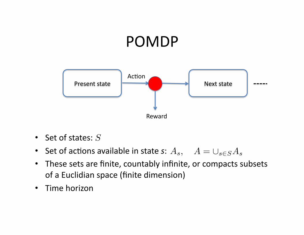
POMDP 

Present state  Next state Ac&on 

Reward 

•  Set of states: •  Set of ac&ons available in state s: •  These sets are finite, countably infinite, or compacts subsets 

of a Euclidian space (finite dimension) 

•  Time horizon  

S

As, A = ∪s∈SAs

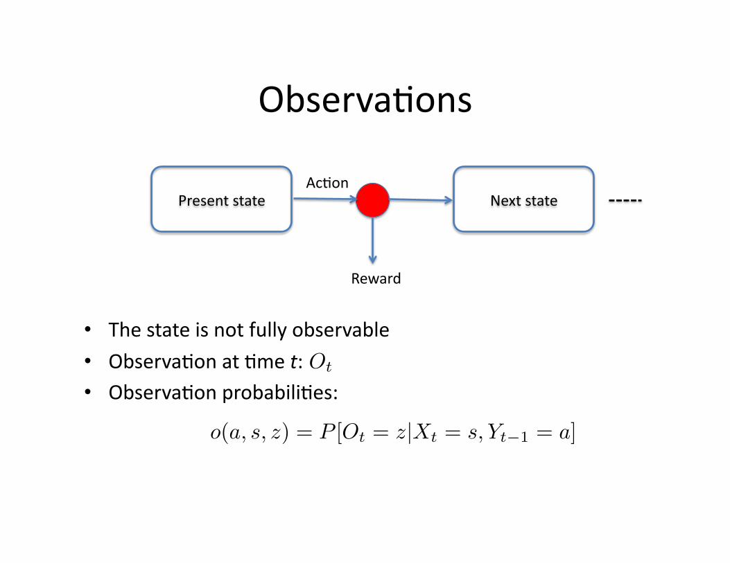
Observa&ons 

Present state  Next state Ac&on 

Reward 

•  The state is not fully observable •  Observa&on at &me t:  •  Observa&on probabili&es: 

Ot

o(a, s, z) = P [Ot = z|Xt = s, Yt−1 = a]

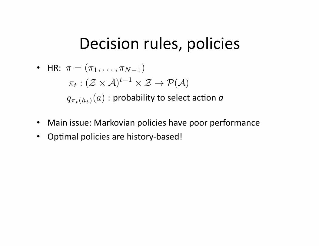
Decision rules, policies •  HR: 

•  Main issue: Markovian policies have poor performance 

•  Op&mal policies are history‐based! 

π = (π1, . . . ,πN−1)

qπt(ht)(a) : probability to select ac&on a  

πt : (Z ×A)t−1 × Z → P(A)

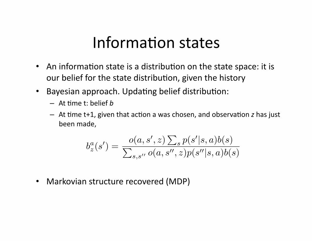
Informa&on states •  An informa&on state is a distribu&on on the state space: it is 

our belief for the state distribu&on, given the history 

•  Bayesian approach. Upda&ng belief distribu&on: –  At &me t: belief b 

–  At &me t+1, given that ac&on a was chosen, and observa&on z has just been made, 

•  Markovian structure recovered (MDP) 

baz(s′) =

o(a, s′, z)∑

s p(s′|s, a)b(s)∑

s,s′′ o(a, s′′, z)p(s′′|s, a)b(s)

More on POMDP •  Read Anthony Cassandra’s thesis:  “Exact and Approximate Algorithms for POMDP” 

Limit theorems •  Read Kushner Dupuis book:  “Numerical methods for stochas&c control problems in con&nuous &me” 

•   … or Kushner’s paper (same &tle), SIAM J. Control and Op&miza&on, 1990 

An example 

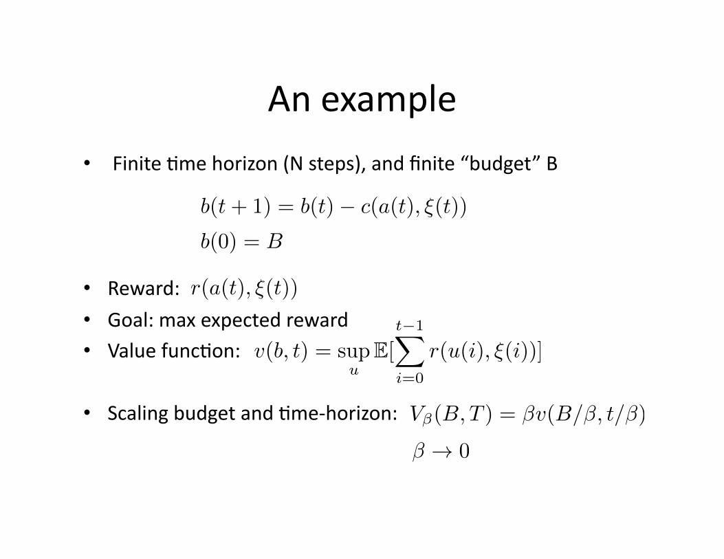
•   Finite &me horizon (N steps), and finite “budget” B 

•  Reward: •  Goal: max expected reward •  Value func&on: 

•  Scaling budget and &me‐horizon:    

b(t+ 1) = b(t)− c(a(t), ξ(t))

r(a(t), ξ(t))

b(0) = B

v(b, t) = supu

E[t−1∑

i=0

r(u(i), ξ(i))]

Vβ(B, T ) = βv(B/β, t/β)

β → 0

An example 

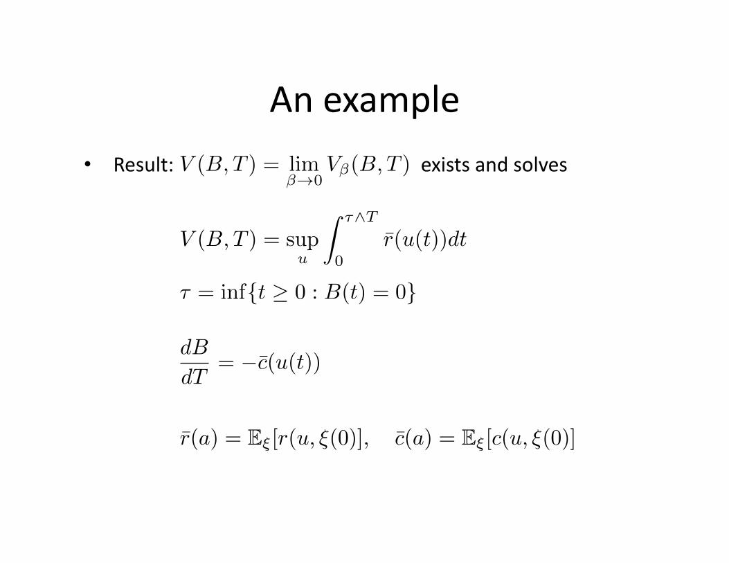
•   Result:                                                  exists and solves   V (B, T ) = limβ→0

Vβ(B, T )

V (B, T ) = supu

∫ τ∧T

0r̄(u(t))dt

τ = inf{t ≥ 0 : B(t) = 0}

dB

dT= −c̄(u(t))

r̄(a) = Eξ[r(u, ξ(0)], c̄(a) = Eξ[c(u, ξ(0)]

Mul&‐Armed Bandit (MAB) 

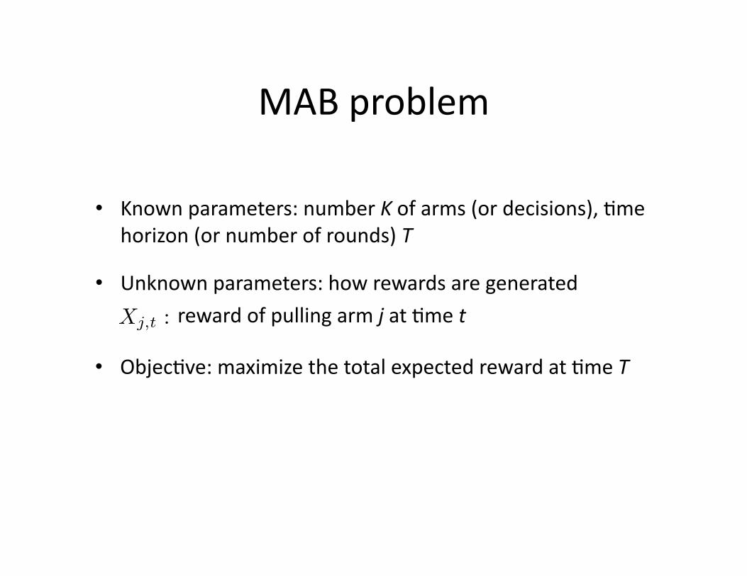
MAB problem 

•  Known parameters: number K of arms (or decisions), &me horizon (or number of rounds) T 

•  Unknown parameters: how rewards are generated 

        reward of pulling arm j at &me t 

•  Objec&ve: maximize the total expected reward at &me T 

Xj,t :

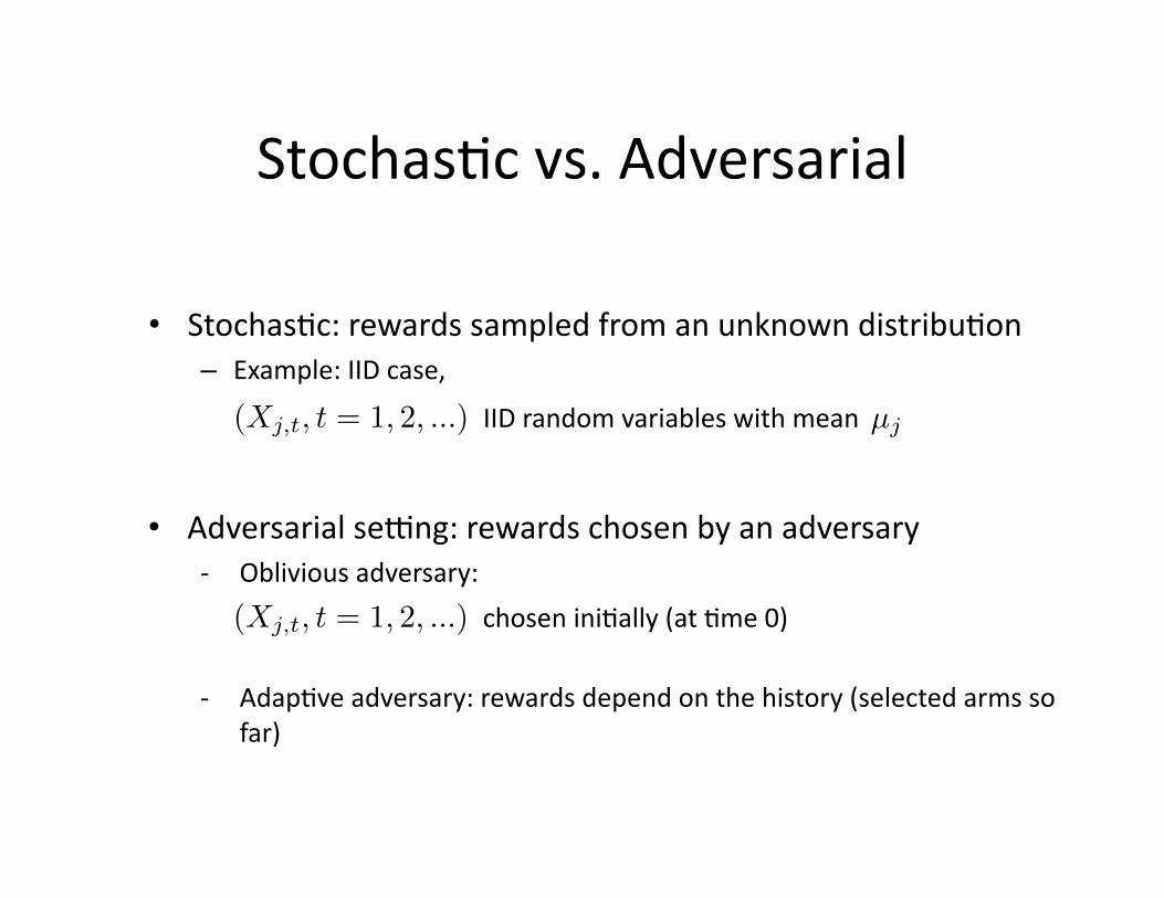
Stochas&c vs. Adversarial 

•  Stochas&c: rewards sampled from an unknown distribu&on –  Example: IID case, 

•  Adversarial sedng: rewards chosen by an adversary ‐  Oblivious adversary: 

‐  Adap&ve adversary: rewards depend on the history (selected arms so far) 

(Xj,t, t = 1, 2, ...) µjIID random variables with mean 

(Xj,t, t = 1, 2, ...) chosen ini&ally (at &me 0)  

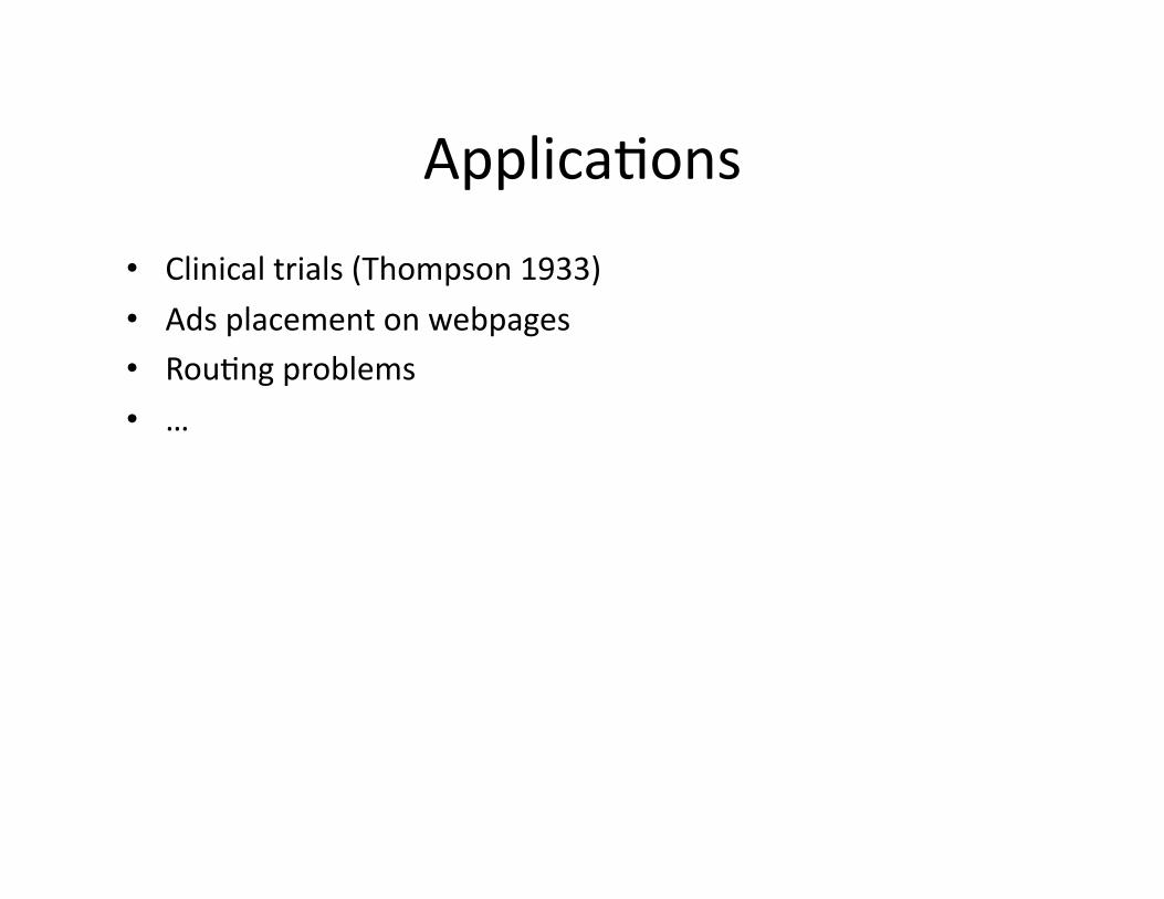
Applica&ons 

•  Clinical trials (Thompson 1933) 

•  Ads placement on webpages •  Rou&ng problems 

•  … 

Outline of the next lectures 

•  Asympto&cally op&mal policies for IID MAB + UCB policies 

•  Finite‐&me analysis of IID MAB •  Large number of arms 

–  Unstructured rewards –  Structured rewards 

•  Adversarial MAB 

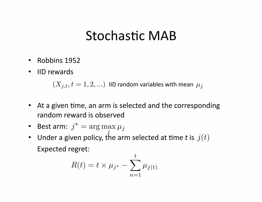
Stochas&c MAB 

•  Robbins 1952 •  IID rewards 

•  At a given &me, an arm is selected and the corresponding random reward is observed 

•  Best arm: •  Under a given policy, the arm selected at &me t is 

 Expected regret:  

(Xj,t, t = 1, 2, ...) µjIID random variables with mean 

j! = argmaxj

µj

j(t)

R(t) = t× µj! −t∑

n=1

µj(t)

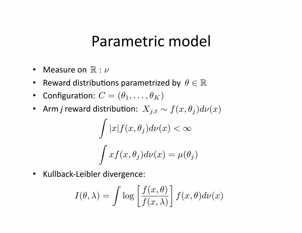
Parametric model 

•  Measure on  

•  Reward distribu&ons parametrized by •  Configura&on:  •  Arm j reward distribu&on: 

•  Kullback‐Leibler divergence: 

R : ν

θ ∈ RC = (θ1, . . . , θK)

Xj,t ∼ f(x, θj)dν(x)∫|x|f(x, θj)dν(x) < ∞

∫xf(x, θj)dν(x) = µ(θj)

I(θ,λ) =

∫log

[f(x, θ)

f(x,λ)

]f(x, θ)dν(x)

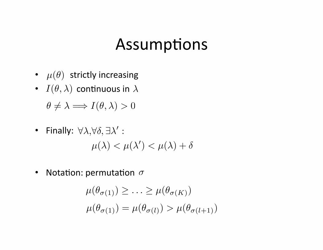
Assump&ons 

•             strictly increasing •                con&nuous in 

•  Finally: 

•  Nota&on: permuta&on     

µ(θ)

θ != λ =⇒ I(θ,λ) > 0

I(θ,λ) λ

∀λ,∀δ, ∃λ′ :

µ(λ) < µ(λ′) < µ(λ) + δ

σ

µ(θσ(1)) ≥ . . . ≥ µ(θσ(K))

µ(θσ(1)) = µ(θσ(l)) > µ(θσ(l+1))

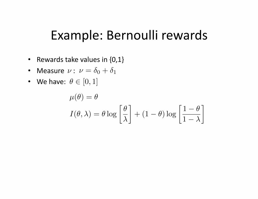
Example: Bernoulli rewards 

•  Rewards take values in {0,1} •  Measure     :        •  We have:  

ν

θ ∈ [0, 1]

ν = δ0 + δ1

µ(θ) = θ

I(θ,λ) = θ log

[θ

λ

]+ (1− θ) log

[1− θ

1− λ

]

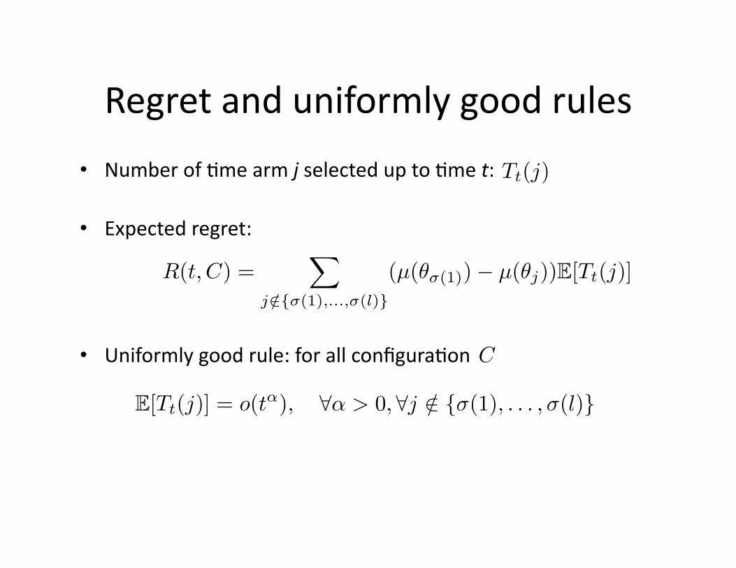
Regret and uniformly good rules 

•  Number of &me arm j selected up to &me t: 

•  Expected regret: 

•  Uniformly good rule: for all configura&on  

Tt(j)

R(t, C) =∑

j /∈{σ(1),...,σ(l)}

(µ(θσ(1))− µ(θj))E[Tt(j)]

C

E[Tt(j)] = o(tα), ∀α > 0, ∀j /∈ {σ(1), . . . ,σ(l)}

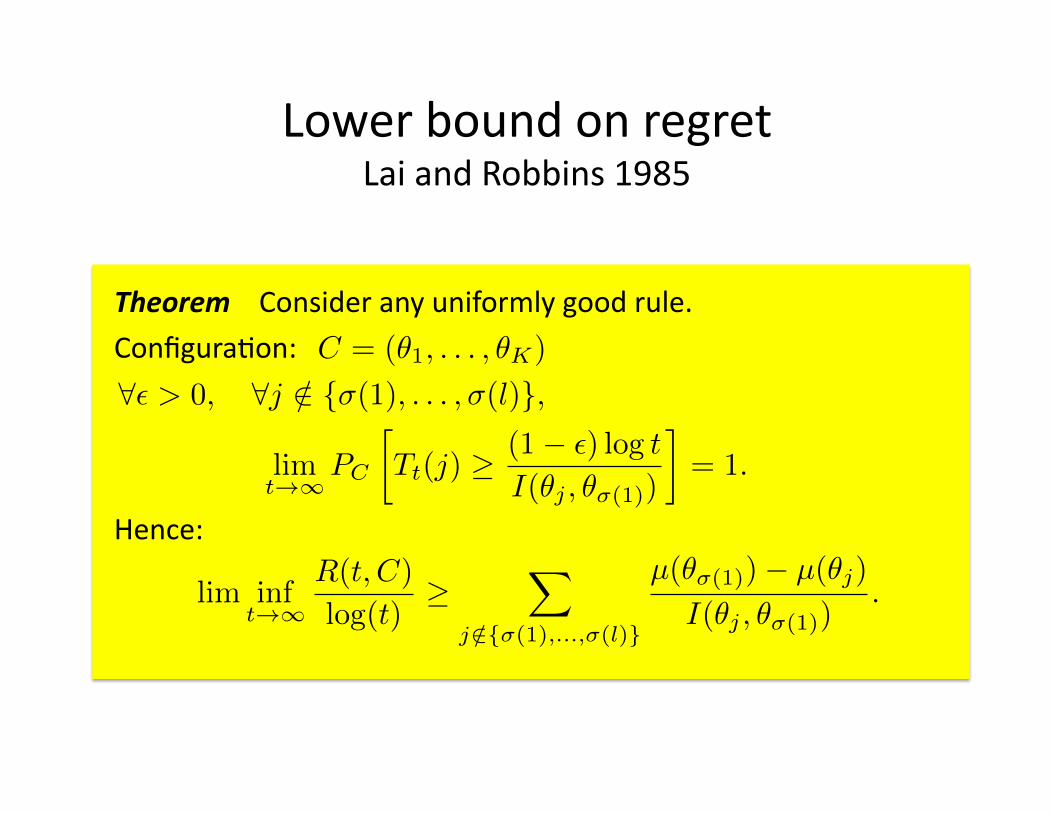
Lower bound on regret Lai and Robbins 1985 

Theorem    Consider any uniformly good rule.  

Configura&on:  

Hence: 

C = (θ1, . . . , θK)

∀ε > 0, ∀j /∈ {σ(1), . . . ,σ(l)},

limt→∞

PC

[Tt(j) ≥

(1− ε) log t

I(θj , θσ(1))

]= 1.

lim inft→∞

R(t, C)

log(t)≥

∑

j /∈{σ(1),...,σ(l)}

µ(θσ(1))− µ(θj)

I(θj , θσ(1)).

Universality of the bound 

•  Similar bound can be derived for controlled Markov chains, i.e., for parametrized average reward MDP 

•  Graves‐Lai 1996. Asympto&cally efficient adap&ve choice of control laws in controlled Markov chains.  

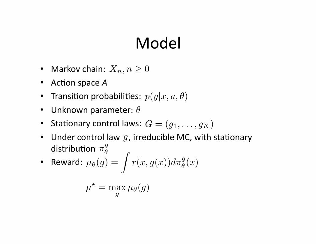
Model •  Markov chain: 

•  Ac&on space A •  Transi&on probabili&es: •  Unknown parameter: •  Sta&onary control laws: •  Under control law    , irreducible MC, with sta&onary 

distribu&on •  Reward:    

Xn, n ≥ 0

p(y|x, a, θ)θ

G = (g1, . . . , gK)

gπgθ

µθ(g) =

∫r(x, g(x))dπg

θ (x)

µ! = maxg

µθ(g)

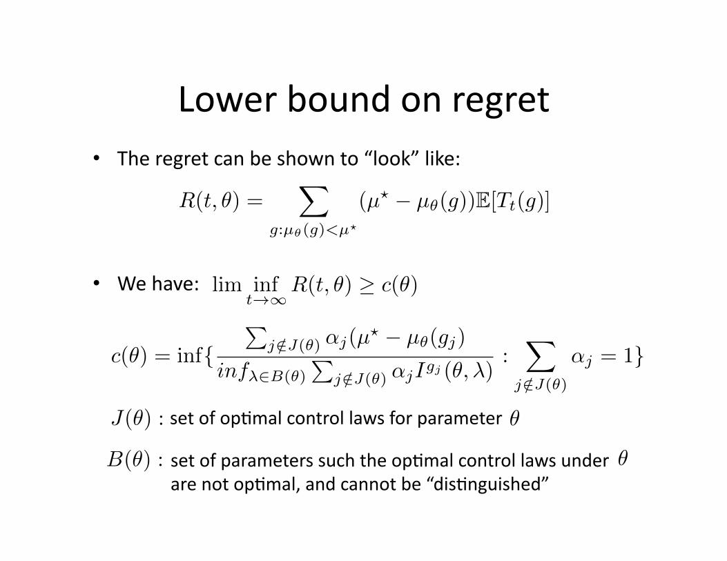
Lower bound on regret •  The regret can be shown to “look” like: 

•  We have: 

R(t, θ) =∑

g:µθ(g)<µ"

(µ! − µθ(g))E[Tt(g)]

lim inft→∞

R(t, θ) ≥ c(θ)

c(θ) = inf{∑

j /∈J(θ) αj(µ" − µθ(gj)

infλ∈B(θ)

∑j /∈J(θ) αjIgj (θ,λ)

:∑

j /∈J(θ)

αj = 1}

J(θ) :

B(θ) :

set of op&mal control laws for parameter  θ

set of parameters such the op&mal control laws under  are not op&mal, and cannot be “dis&nguished”  

θ