separating moral hazard from adverse selection in

Separating Moral Hazard from Adverse Selection in

Automobile Insurance: Longitudinal Evidence from France∗

Georges Dionne Pierre-Carl Michaud Maki Dahchour

Working paper 04-05 Canada Research Chair in Risk Management, HEC Montréal

August 26, 2004

AbstractThis paper uses longitudinal data to perform tests of asymmetric information

in the French automobile insurance market for the 1995-1997 period. This marketis characterized by the presence of a regulated experience-rating scheme (bonus-malus). We demonstrate that the result of the test depends crucially on howthe dynamic process between insurance claims and contract choice is modelled.We apply a Granger causality test controlling for the unobservables. We findevidence of moral hazard which we distinguish from adverse selection using amultivariate dynamic panel data model. Experience rating appears to lead highrisk policyholders to choose contracts that involve less coverage over time. Thesepolicyholders respond to contract changes by increasing their unobservable effortsto reduce claims.

JEL CODES: D80, G22, C23, L51.KEYWORDS: Automobile insurance, road safety, asymmetric information, experience rat-

ing, moral hazard, adverse selection, dynamic panel data models, Granger causality test.

∗G. Dionne, Canada Research Chair in Risk Management, HEC Montréal, [email protected]. Michaud, Ph.D student, CentER, Tilburg University and Research Affiliate IZABonn, [email protected]. M. Dahchour, Aviva Canada, National Personal Lines,[email protected]. Earlier versions of the paper benefited from comments made byJaap Abbring, Charles Bellemare, Denis Bolduc, Sylvain Lassarre, Jean Pinquet, Arthur van Soest,and Frank Windmeijer; by participants at the “Sécurité routière et assurance automobile” symposiumFFSA (Paris, December 18th 2000), at the 41st Congress of the Société Canadienne de ScienceÉconomique (Québec, May 15-16th 2001) and at the European Meeting of the Econometric Society(Madrid, August 20-24th 2004), and seminar participants at Tinbergen Institute Amsterdam andTilburg University. Financial support by INRETS, CRSH, and FFSA is acknowledged. Part of thispaper was written while the second author was visiting the Institute for Fiscal Studies and the Laborand Population group at RAND Corporation, whose hospitality is gratefully acknowledged.

1

1 Introduction

In France, automobile insurance pricing is based on two elements. The first is a so-calleda priori pricing system which consists in constructing classes of homogeneous risks basedon the characteristics of policyholders. The second is an a posteriori pricing mechanismor experience-rating scheme called bonus-malus, where past at-fault accidents are usedto adjust the premium in the next periods.The insurance industry is fully committed to the application of the bonus-malus

scheme and this commitment is in fact enforced by a law stipulating that each insurermust apply the same bonus-malus formula for similar driving histories according to rulesthat cannot be renegotiated. Over the last decade, regimes of this sort have come undercriticism from the European Commission, on several grounds (Council of EuropeanCommunities, 1992; Picard, 2000). One specific criticism is that such pricing schemesreduce competition among insurers. In its analysis, the Commission did not, however,take into account the value of the scheme’s commitment to enforcing optimal incentivecontracts in the presence of asymmetric information.Experience rating works at two levels. Since past accidents implicitly reflect unob-

servable characteristics of drivers (e.g. their driving skills) and introduce safe-drivingincentives, experience rating can help in responding directly to the problems of adverseselection and moral hazard which often disturb the insurance market’s allocation of risk.(Dionne, 2001). To confirm the need for such a multi-period scheme, we must prove theexistence of residual asymmetric information in single-period contracting. Puelz andSnow (1994) tested for the presence of adverse selection in the portfolio of an Americaninsurer. Their idea was to take a risk profile observable by the insurer and look fora positive correlation between insurance claims and levels of insurance coverage. Theseminal theories of Rothschild and Stiglitz (1976) and Wilson (1997) do strongly predictthat such a correlation should be observed in the data. Puelz and Snow (1994) concludedthat there was adverse selection in the contractual relationships they looked at. But thesame correlation between insurance coverage and claims can also be explained by moralhazard or even heterogeneous risk aversion (Chiappori et al., 2004).Dionne, Gouriéroux, and Vanasse (2001) have shown that the Puelz-Snow results

(1994) were probably derived from incomplete specification of the econometric model.These authors found no evidence of residual asymmetric information when testing fornon-linearities in insurance pricing with a model based on similar data from a Canadianinsurer. They also pointed out that heterogeneous risk aversion was captured by anumber of observable classification variables. Chiappori and Salanié (2000) came tothe same conclusion concerning residual asymmetric information when looking at datacollected from French insurers on the claims policyholders filed in 1990. Needless tosay, this lack of evidence for the presence of residual asymmetric information in the

2

automobile insurance market is somewhat puzzling. And especially it is so, seeing thatthe insurance industry seems of the common opinion that the additional use of experiencerating for insurance pricing is crucial in responding to information problems. However,it could be that moral hazard and adverse selection work in opposite directions whenno means are found to control for certain unobservable factors. Single-period data oncontracts may not provide sufficient instruments to separate the two problems.Studies by Chiappori (2000) and Chiappori and Salanié (2000) have clearly shown

that tests using the Puelz-Snow methodology (1994) fail to distinguish between ad-verse selection and moral hazard. Such tests give only a global view of the presence ofasymmetric information. Experience rating, by contrast, not only provides additionalinformation on risk classification but may also play an important role in the dynamicrelationship between policyholders’ insurance claims and contract choice (Dionne, 2001).The theoretical literature clearly indicates that these features may help overcome prob-lems of moral hazard when risks known to the policyholder (endogenous) are unobserv-able by the insurer (Winter, 2000).In France, contract choice is influenced by the evolution of the premium which, by

law, is itself closely linked to the policyholder’s driving record. Since increased insurancecoverage tends to lower the expected costs of accidents, incentives for safe driving isweakened for all risks. Under experience rating, the subsequent rise in accidents increasesthe marginal costs of future accidents. Hence, experience rating may help in correctingthe disincentive effect created by single-period insurance coverage. Since results obtainedby Chiappori and Salanié (2000) can be interpreted as evidence that there is no residualasymmetric information problem in the French automobile insurance market, the benefitsof experience rating mitigating moral hazard can also be called into question. However,these tests were conducted in a static framework which fails to recognize the dynamicsthat experience rating and semi-commitment introduce into contractual relationships.Abbring et al. (2003a) have made a recent attempt to apply this multi-period in-

centive mechanism, by focusing on the dynamics of claims but not on the dynamics ofcontract choice (because of data limitations). Applying specific assumptions about thewealth effects of accidents to policyholders who differ only in their claims record (thustheir experience rating), their model predicts that subjects with the worst claims recordsshould try harder to drive safely and thereby, ceteris paribus, file fewer claims. Yet, theirdata do not support the presence of moral hazard. After all, the puzzle identified byChiappori and Salanié (2000) and Dionne, Gouriéroux, and Vanasse (2001) remains un-solved. Does no residual asymmetric information mean no residual moral hazard andno residual adverse selection?In this paper, we shall show that failure to detect residual asymmetric information

and, more specifically, moral hazard in insurance data and, potentially, in other data

3

sets, is due to the failure of previous econometric approaches to model adequately thedynamic relationship between contract choice and claims when looking at experiencerating. Using a unique longitudinal survey of policyholders from France, we show that,as anticipated by Chiappori and Salanié (2000), omission of the experience-rating vari-able most plausibly explains the failure to detect asymmetric information in tests similarto the one they applied. The bonus-malus coefficient is, indeed, negatively related tothe level of insurance coverage (through fluctuations in the premium) and positively cor-related to claims (potentially through unobserved heterogeneity). The coefficient thusappears to hide the link between claims and contract choice which is exactly what Chi-appori and Salanié (2000) had in mind. This is apparent in traditional cross-sectionaltests as well as in extrapolations using longitudinal data models that simply pool re-peated observations or permit the correlation of unobserved independent factors witheach contract observed over time. For our data set, these factors essentially improve thepower of the test to detect asymmetric information.This paper also proposes a methodology to disentangle the historical pathways which

lead asymmetric information to a conditional correlation between claims and levels ofcoverage. Within a longitudinal data framework controlling for unobservables (Chamber-lain, 1984), we show how Granger causality (Granger, 1969) can be used to disentanglemoral hazard from adverse selection. We argue that this test is the most appropri-ate in insurance markets characterized by semi-commitment, where full anticipation oflong-run behavior is not optimal.We find evidence of Granger causality linking insurance coverage with accident rates

in following years and this points to the presence of moral hazard. After filing at-faultclaims or receiving premium increases, policyholders reduce their level of coverage andtry harder to substantially reduce their likelihood of filing any future claims. In our dataset, a switch from all-risk coverage (costs covered for both parties) to limited coverage(only third-party costs) is associated with a substantial 6% decline in the probability aclaim will be filed.We also find that there is no presence of residual contemporaneous asymmetric infor-

mation in the data. From our results, it appears that a priori classification can accountfor the unobservable risk characteristics of policyholders if insurers have access to expe-rience rating as an additional source of information in assessing the risk profiles of theirclients. Indeed, we find that the change in contract is most often triggered by a risingexperience rating coefficient.The paper is organized as follows. In section 2, we present key features of the French

automobile insurance market and discuss important issues regarding the regulatory con-text within which tests of asymmetric information are made. In section 3, we presentthe data used in our analysis and examine their main features. In section 4, we repli-

4

cate methodologies similar to those of Chiappori and Salanié (2000) and Dionne et al.(2001) for each cross-section but also for the panel data examining the effect of omittedvariables, (especially experience rating) on test conclusions. In section 5, we performGranger causality test for moral hazard and adverse selection. Section 6 concludes.

2 The French Automobile Insurance Market

To understand how one can study empirically asymmetric information in the French au-tomobile insurance market, it is important to start with a description of the institutionalsetting peculiar to France.1

Exclusivity and Semi-commitment – There is no clause in insurance contracts“forcing” drivers to stay with the same insurance company once the contractual periodis over or even during a contractual period. However, there is some exclusivity writteninto insurance contracts, in that a policyholder cannot have contracts with differentinsurers to insure the same risk in a given period. Hence, only semi-commitment ispossible in this market. It is not optimal for a policyholder to commit to multiperiodarrangements with one insurer, since there is the possibility of renegotiating contractsand switching insurer. This is common to many insurance markets. (On the notion ofcommitment, see Dionne and Doherty, 1994, and Hendel and Lizzeri, 2003).

Experience Rating Law–According to the regulations in force in France (Article A121-1 - Automobile insurance - Reduction-Increase clause of the French Insurance Codeand its appendix), the premium charged to the policyholder is necessarily determinedby multiplying the amount of the a priori premium by a so-called reduction-increasecoefficient.2 The base coefficient is 1. After each year of accident-free insurance coverage,the coefficient applied is that of the preceding contract period minus 5%. Each at-faultaccident occurring within the insurance year will increase the coefficient by 25%. Theclause also stipulates that there will be no increase for the first accident occurring aftera period of at least three years during which the bonus-malus coefficient was equal to0.50.

Public Information on Accidents – At-fault claims filed by drivers fall into thedomain of public information to which rival companies have free access. Bonus-malusinformation must be reported when the subscriber purchases a new insurance contract.

1See Richaudeau (1998), Picard (2000), Dionne (2001), and Fombaron (2002) for a detailed descrip-tion of the automobile insurance market in France and Pinquet (1999) for an analysis of the experiencerating.

2Throughout this paper, this coefficient will be referred to as the bonus-malus coefficient, meaningthat it counts as a bonus when less than 1 but as a malus when more than 1.

5

Moreover, since experience rating is enforced by law, the industry is fully committed toapplication of the bonus-malus scheme.

This commitment on the part of insurers is crucial. Theoretical studies haveshown that, failing commitment on the insurer’s part, the bonus-malus scheme will pro-vide no incentive whatsoever (Chiappori et al., 1994). Similarly, any benefits from thebonus-malus will be eliminated if a particular insurance company acquires an informa-tional edge from access to private data on its clients’ accidents. Drivers will then chooseanother insurer when the malus increases (Kunreuther and Pauly, 1985; Dionne andDoherty, 1994; Fombaron, 1997). Finally, evidence seems to show that there is fullcompetition among insurers regarding the a priori pricing of insurance.

Types of Insurance Coverage– Two types of insurance coverage predominate: all-risk insurance (tous risques) and third-party liability (responsabilité civile). The formerinsures against losses incurred by both the policyholder and the third-party, whereasthe latter, as its name indicates, insures only against third-party losses. At minimum,the law prescribes that a policyholder must have a limited third-party insurance policy.Chiappori and Salanié (2000) report an average annual premium of 3000 Francs (1986Francs) for this coverage, whereas the premium for all-risk insurance coverage coststwice as much and increases with the value of the vehicle. Hence, the choice of insurancecoverage is an important decision for policyholders.

To summarize, the institutional setting of the French automobile insurance mar-ket corresponds to dynamic models characterized by renegotiation and semi-commitment.As already argued, this setting introduces testable predictions of the effects of asym-metric information on contractual relationships. In such a setting, where insurers arecommitted and the policyholder’s driving record is public information, the experiencerating scheme can be expected to promote safe driving and to serve as a useful tool inclassifying the riskiness of drivers.

3 The SOFRES Longitudinal Survey

The SOFRES longitudinal survey covers a representative sample of French drivers from1995 to 1997 (3 years).3 The information available in the database is composed of threeelements. The first concerns information on driver characteristics (sex, age, number ofaccidents). The second covers the vehicles (year, group, etc.). The third and most impor-tant element for the problem we are studying relates to insurance contracts. It providesthe bonus-malus coefficient and the type of insurance coverage. These two variables rep-resent a very good proxy for actual insurance contract characteristics. Unfortunately,

3See chapter 6 of Dahchour (2002) for a detailed description of the database.

6

information on other characteristics of the contract is very limited, containing nothingabout insurance premiums or deductibles, let alone anything about the identity of theinsurer from year to year. Though ideally, one would prefer to have such information,the choice between “all-risk” insurance or “third-party” is likely to be the most impor-tant decision for the policyholder. In fact, the level of deductible seems mainly relatedto the value of the vehicle.Our final sample is thus a three-year incomplete panel (1995-1997). We define an

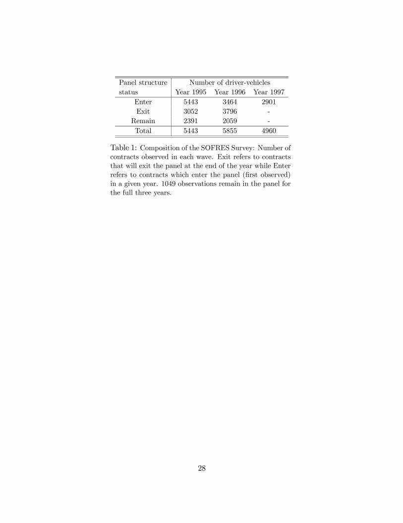
observational unit as a policyholder along with a vehicle defined by the first 4 digitsof its license number plus the year the car was manufactured.4 A policyholder is notnecessarily present in each year. Indeed, many contracts are observed for less than threeyears. Table 1 gives the structure of the panel, with its entries and exits.

[Table 1 about here]

Using surveys based on policyholder records has two main advantages. The first isthat, since attrition is presumably much less problematic than with insurers’ portfolios,the representability of the panel might be expected to remain constant over time. Inthe case of data provided by insurers, the reason prompting a policyholder to switchinsurers might well be the changing terms of his contract, which is precisely the subjectunder investigation in this literature. In our case, although we cannot observe theidentity of the insurer, we do not lose track of contracts that are switched so long as thepolicyholder keeps the same vehicle. Therefore, no observational unit need be censoredbecause drivers change insurers. However, if the decision to change a vehicle is correlatedwith changes in contract parameters, then there might still be an attrition bias. (Welook into that possibility in Section 4 but fail to confirm that suspicion.) Furthermore,we use entrants in 1996 and 1997 to maintain the representability of the sample, thuslimiting any loss in efficiency as the yearly sample sizes decrease.The second advantage relates to the observability of both claimed and unclaimed

accidents, one which provides a window for the analysis of reporting behavior. Sincethe contract party reporting accidents is the policyholder, both unclaimed and claimedaccidents involving material damage and injuries are reported. Although this is notthe primary concern of the present investigation, the availability of such information isprecious, because it leads to a better interpretation of the results, making it possible toseparate a drop in accidents from the underreporting of claims.

4In constructing the panel we had to match vehicles with policyholders drawn from different filesfor each year. We merged policyholder IDs with a car identifier consisting of the first 4 digits of theautomobile identification number plus the year in which it was manufactured. This produced a matchquality which minimized the possibility of matching errors while allowing us to trace contracts acrossyears. In what follows, we use the term contract to denote an observational unit.

7

3.1 Contract Characteristics

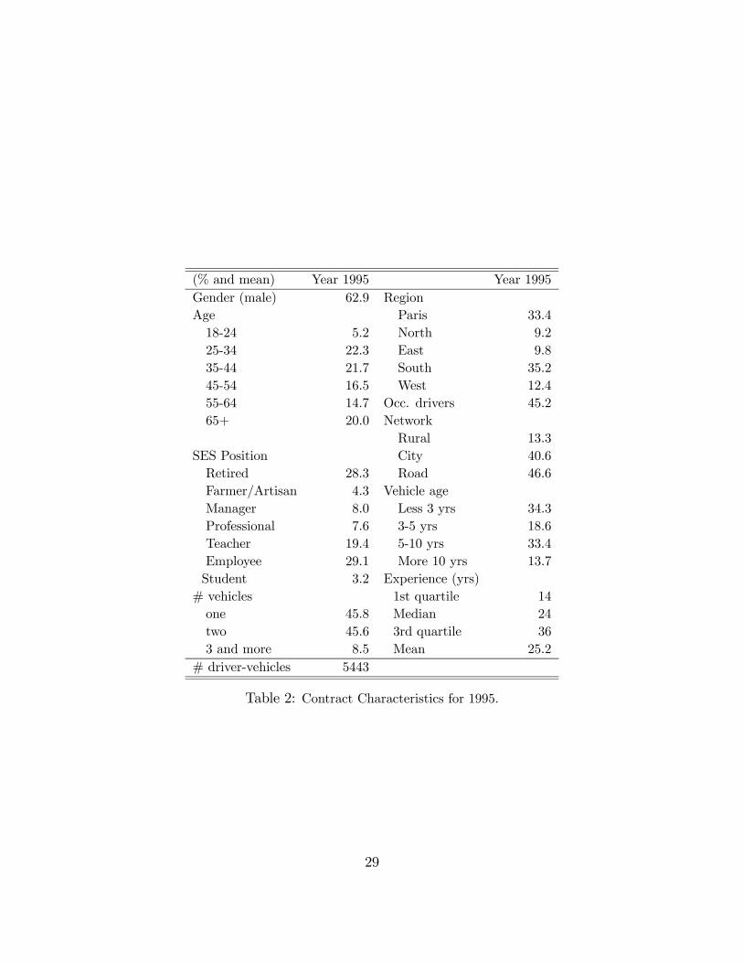
The SOFRES survey provides relatively rich source of information to classify policy-holders and their vehicle. This is highly important for the empirical investigation ofasymmetric information, because the econometrician must try to replicate what the in-surer can know about the policyholder’s risk in order to price insurance. A subset of thecontract characteristics that we use are described in Table 2 for 1995. These have beendocumented elsewhere to be fairly representative of the risk classification variables thatinsurers use for a priori classification (see Dahchour, 2002 chap. 2).


It should be noted that the panel is generally representative of French drivers al-though young drivers are underepresented. This can be explained by the fact that youngdrivers are often included on their parents’ insurance policies, as occasional drivers. In-deed, 45.2% of 1995 contracts feature the presence of occasional users. Policyholdershave, on average, 25 years of experience and relatively few have less than 2 years ofexperience. Regional and socio-economic status (SES) is fairly representative of thepopulation. Policyholders mostly use city and highway networks, although a small pro-portion use rural networks. More than half of the respondents have more than onevehicle; one-third of the vehicles being less than three years old. Yet, a sizeable propor-tion of vehicles are older than five years.

3.2 Bonus-Malus, Accidents and Insurance Coverage

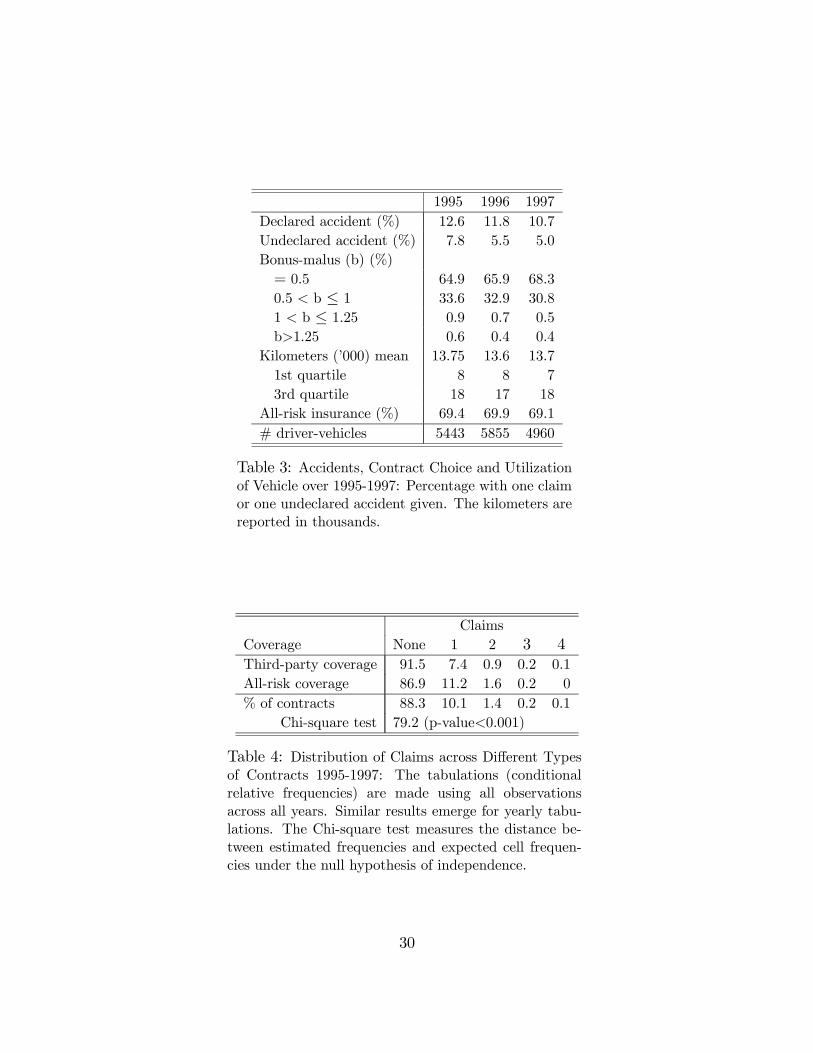
The evolution of the key variables used to study the dynamics in insurance contractchoices and accidents is given in Table 3.


The percentage of policyholders reporting at least one claim in a given year is 12.6% in1995. Undeclared accidents are much less frequent. An estimated 7.8% of policyholdersdid not report an accident in 1995 and this relative frequency decreases to 5% in 1997.The bonus-malus is the coefficient applicable at the beginning of the contractual year.

Therefore, it does not take into account claims in the current year. Nearly two-thirdsof policyholders have a maximal bonus (or minimal bonus-malus) coefficient while veryfew have one in excess of 1. Indeed, the law prescribes that a policyholder cannot havea bonus-malus in excess of unity after three years without at-fault claims.The mean exposure to risk, measured by the number of kilometers the vehicle was

used, does not change over the period. On average policyholders report driving their

8

vehicle about 13,700 km per year, while three quarters of policyholders use their vehicleless than 18,000 km per year. Finally, more than two-thirds (69%) of the contractsobserved are all-risk insurance contracts.Before proceeding with tests for residual asymmetric information in this insurance

market, we first document correlation and dependence patterns among the main variablesof interest. In Table 4, we look at how the distribution of claims varies by type ofinsurance coverage.


A first observation is that there are very few contracts which feature multiple claimswithin a year. The relative frequencies show that types of contracts and claims donot appear to be unconditionally independent of the number of claims (Chi-square =79.2, p-value<0.001). Those with all-risk coverage tend to file more claims. All-riskpolicyholders have a 4.6% higher claim incidence than do those with third-party coverage.We should stress that this is not an indication of asymmetric information in contrac-

tual relationships as Dionne, Gouriéroux, and Vanasse (2001) noted. Insurers gatherinformation on policyholders so as to price their policies differentially, with an actuarialfairness that restores an efficient allocation of risk. Therefore, one must look within arisk class, as defined by the characteristics insurers can observe in policyholders (for ex-ample those in Table 2), to see whether or not there is any correlation between contractchoice and claims (Crocker and Snow, 1986). We shall perform such an exercise in thenext section.To get a better understanding of how contract choices, experience rating, exposure to

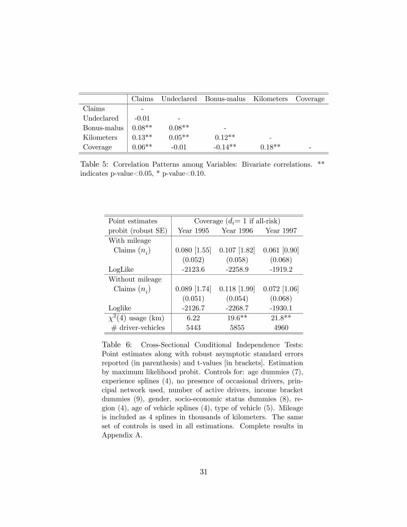
risk (mileage), and the decision to file a claim interact, we can look at rough correlationsamong these variables. In Table 5, bivariate correlations are reported.


These correlations and the information in Table 4 tend to illustrate the three mainpoints made about the bonus-malus by many observers. (See Picard (2000) for ananalysis of deregulation in Europe).First, it is believed that experience-rating schemes lead to inflation of a priori pre-

miums for drivers with a limited or poor driving history. Some insurers may indeed takeadvantage of the experience rating regulation to manipulate a priori pricing based on theevolution of the bonus-malus.5 In Table 5, the correlation between the bonus-malus and

5Some evidence is provided in an experiment performed by the magazine Que Choisir (November,1998). For identical individuals who only differed in their bonus-malus coefficient, there was considerableheterogeneity in the premium offered across insurance companies, over and above what is mandated bya posteriori pricing, suggesting that the bonus malus may also be used in a priori pricing.

9

contract choice (coverage where 1 is for all-risk coverage) is negative and strongly sig-nificant. However, the bonus-malus is positively correlated to claims, plausibly throughnon-observable heterogeneity.Second, one of the common characteristic of these schemes is that they penalize

less than reward, resulting in some sort of “forced” risk pooling at the lowest-end ofthe experience-rating distribution. From Table 4, we see that more than two-thirds ofpolicyholders are at the lower end of the distribution. Very few policyholders have abonus-malus above 1. It is thus difficult, for low risks with the best records, to separatethemselves from high risks with similar experience-rating coefficients. Over and abovewhat is prescribed by law, some insurers may even use specific rebates that reduce the“effective” bonus-malus coefficient to its lowest limit of 0.5.6

Third, since the penalty for a claim where the driver is at fault does not take intoaccount of the size of the claim, small claims that would otherwise be reported may notbe under experience rating and this adds to the possibility of cross-subsidization. We geta glimpse of this from Table 5 if we take the correlation between undeclared accidentsand the bonus-malus. The correlation is positive and statistically significant indicatingthat those with a higher bonus-malus may tend to refrain from filing a claim.In summary, all these stylized observations tend to suggest that experience-rating

schemes introduce dynamic mechanisms, where contract choice and claims depend onthe evolution of experience-rating coefficients which in turn depend on the past decisionsof the contractual parties. There appears to be a somewhat “dangerous” triangularcorrelation between claims, contract choice, and the experience-rating coefficient. Thiscan confuse the correlation between claims and contract choice within risk profiles, acorrelation which is crucial for testing asymmetric information, as we shall see in thenext section.

4 Presence of Asymmetric Information

4.1 Cross-Sectional Data Test

Based on a traditional conditional independence test, one can use a cross-section of pol-icyholders along with their characteristics to test whether those with high unobservablerisk have more coverage. If there is asymmetric information in a contractual relation-ship then, within a risk class summarized by a vector of the policyholder’s characteristicswhich are observable to both parties, xi, the residual unobserved variation in risk andcontract choice should be correlated. This is a robust prediction from the adverse se-

6Some analysts even argue that the effective coefficient might be below 0.5.

10

lection and/or moral hazard literature, as applicable to the setting described in theintroduction. As already discussed, such single period tests are designed to detect thepresence of residual asymmetric information, since they cannot disentangle moral hazardfrom adverse selection.Denote by di the contract choice of policyholder i and ni the number of claims. Then,

conditional independence holds under

H0 : F (di|xi, ni; θd) = F (di|xi; θd) (1)

given θd is some finite-dimensional parameters vector and F is the cumulative dis-tribution function (cdf) of di conditional on xi. Relation (1) means that the numberof claims does not give information on the distribution of contract choice (Dionne etal., 2001). In other words, under the null, there is no residual asymmetric informationwithin a risk class and contract choice does not correlate with claims. If, however, high-risk policyholders would choose more coverage than low risk policyholders under adverseselection or if individuals with more insurance coverage would be less motivated to drivecarefully under moral hazard, then a positive correlation should be observed.A non-parametric test will handle the dreaded dimensionality problem. The vector

xi must be rich enough to represent the insurer’s information set and the data require-ments for generating fixed power to reject the null of conditional independence will growexponentially. In this paper, we opt for a parametric form of the test where

di = I(x0iβd + πnni + udi > 0). (2)

The error term udi follows a distribution that we will assume to be normal but whichcould also be logistic with some rescaling.7 I(.) is the indicator function (I(a) = 1 if a istrue, 0 otherwise) that denotes the choice of a certain insurance coverage (1 is for all-riskcoverage). This could be extended to other types of discrete or continuous choice setsbut available data will generally force a particular choice. In our case, we only observea binary variable for insurance contracts, so we consider a class of binary-choice models.A test for asymmetric information using this parametric model is given by πn = 0

under the null hypothesis of conditional independence and is implemented by estimating(2) on a cross section of N contracts {di, ni,xi}Ni=1.Implicit in (1) is that the model is correctly specified. But, as Dionne, Gouriéroux,

and Vanasse (2001) emphasize, care must be given to the specification of the indexx0iβd. Indeed, it must reflect the insurer’s knowledge of the driver’s situation at the timewhere the contract is negotiated. We use combinations of dummy variables (age, socio-economic status, income, region, road network used, car type, fuel type, number of active

7We investigate the possibility of faulty specification of such a distribution in the next section.

11

drivers) in addition to continuous variables such as the car’s manufacture date and thedriver’s experience. For these variables, we use spline functions with nodes at naturalpoints, given the distribution of the data.8 So, these constitute flexible approximationsto non-linear functions. This is highly important as Chiappori and Salanié (2000) show;even for very simple utility functions, the optimal pricing policy can be quite non-linear.9

Note that, for now, we make no room for using the bonus-malus coefficient in a prioripricing. Hence, we assume that insurers will follow regulations and not use experiencerating to classify policyholders ex-ante.The database also contains data on mileage for the current year. However, the use

of such a variable is problematic: no assumption can be made concerning its evolutionduring the contract year nor can it be observed by the insurer when the contract isnegotiated. Clearly, claims can affect kilometers in the current year. The potential biasresulting from a correlation between the unobservables of contract choice and mileagecan affect the claim coefficient being tested. Insurers use some proxy for kilometers intheir risk classification. For now, we shall report results with and without mileage.Based on the three years of data, Table 6 reports the results for each year with and

without mileage spline variables. Most of the risk-classification controls in the tabletake the anticipated signs (see Appendix A for complete results), while the pseudo R-square varies between 0.35 to 0.38. Results for 1995 and 1997 suggest that we should notreject conditional independence at the 5% level (t0.05=1.96) and hence conclude for theabsence of asymmetric information for both specifications with and without mileage.For 1996, the conclusion depends on the inclusion of the mileage variable. Withoutthis variable there seems to be enough evidence to reject the null. However, once themileage variable is introduced, there seems to be less evidence against the absence ofasymmetric information. The mileage variable is informative about contract choices.This can be seen from comparisons of the likelihoods. For 1996 and 1997, we canreject the restrictions that the four mileage splines included do not provide informationabout contract choice (χ2(4) =19.6 (21.8) for 1996 (1997)) . The causality’s direction ishowever uncertain. Usage can change as a result of contract change or change in plannedusage can encourage the policyholder to modify insurance coverage. Furthermore, asimultaneity bias can lead to a bias in the claim coefficient. This variable obviouslydoes not belong in the insurer’s information set when negotiation takes place. Sinceconclusions across years are ambiguous, we perform some robustness checks to see if a

8For a continuous variable z, the m spline denoted zm with lower node at ψm−1 and ψm will begiven by zm = max(min(z − ψm−1,ψm − ψm−1), 0). In a linear regression of y on z1, ..., zM , the slopefor zm measures the local slope on the segment (ψm−1,ψm). We also experimented with combinationsof splines and binary indicators which did not change results (available upon request).

9We experimented with limited interactions among variables to the extent that the data providesenough variation (involving additional variation in contract choice) to identify their effect.

12

more stable pattern could emerge.


4.2 Robustness Tests

4.2.1 False specification of Functional Form

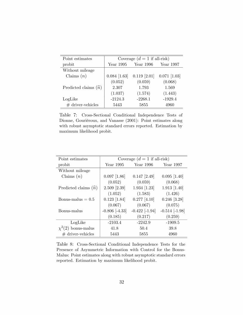
The first check is designed to verify if the rejection of the hypothesis for 1996 is robustto false specification of the functional form of the conditional mean whose general formcan be written as E(di|xi, ni) = F (h(x, ni)). The first object that can be incorrectlyspecified is the index h(xi, ni) inside the distribution function. As proposed by Dionne,Gouriéroux, and Vanasse (2001), we can include best predictor insurers’ of drivers’ claimsin the conditional mean of (2) to see whether any non-linearities and interactions haveescaped the specification used in Table 6.To do so, we estimate, in a first-step, the negative binomial model for the number

of claims in each year, using the same set of risk factors as in the test (since there areno plausible exclusion restrictions).10 We then use estimated parameters to generate aprediction for each year. This prediction is included along with actual claims in theindex of (2). The identification of this effect will come entirely through the exponentialstructure of the prediction. Table 7 reports results for 1995-1997 where we do not includethe mileage variable.11


Contrary to the findings of Dionne, Gouriéroux, and Vanasse, the conclusion of thetest does not appear to depend on the functional form of the index. For 1995, theinclusion of this variable actually helps into increasing the estimate of the parameter onthe claim coefficient but does not affect the conclusion. The conclusion of the test for1996 and 1997 does not change also. One explanation of this negative result may bethat our data set is limited; we do not have access to all insurers’ contract variables asdid Dionne, Gouriéroux, and Vanasse (2001) for a single insurer.10Denote by µit = exp(x

0iπ) the conditional mean of a Poisson distribution of ni. Then it holds true

that V ar(ni|xi) = E(ni|xi) which is usually rejected by the data, the so-called equivariance property.One can assume that µ∗it is given by exp(x

0iπ + νi) and assume that νi follows a gamma distribution

with parameters (δ, δ). This relaxes the equivariance property, since the mixing distribution yields anegative binomial distribution for n (Gouriéroux, Monfort, Trognon, 1984).11In results not reported here, the inclusion of the mileage variable does not change the qualitative

results of this robustness check. Results available upon request.

13

Since the incorrect specification of F (·) is as problematic as that of h(·), we alsotest for normality using the test proposed by Chesher and Irish (1987).12 Interestingly,we cannot reject normality at conventional levels for all the three years (χ2= 1995:10.8,1996:19.8, 1997:24.1 ;χ246,0.95=31.4). We also experimented with exponential forms ofheteroscedasticity by modelling V ar(udi|zi) = exp(z0iφ) for some vector of characteristicszi , but this did not alter the results. All standard errors calculated in Table 6 and 7are robust to unknown forms of heteroscedasticity.Therefore, we conclude that the rejection for 1996 does not appear to come from a

faulty specification of the functional form.

4.2.2 Omitted Variables

A second check is made to see whether there is not an omitted variable which hidesthe link between claims and contract choice. Indeed, Chiappori and Salanié (2000) noteafter finding that drivers with a maximal bonus (0.5) tend to buy more comprehensivecoverage:

“In fact, as our final result on the effect of the bonus coefficient clearly sug-gests, it may be the case that some variable that is observed by the insurersbut somehow is not recorded in our data influences contract choice and risk-iness in opposite directions, and that it cancels out a conditional dependencein our estimates.” (p.72)

What the correlations in Table 5 suggest is that the bonus-malus coefficient itselfmeets this criterion exactly: correlated negatively with contract choice and positivelycorrelated with claims. Table 8 presents the same tests as in Table 7 where we add asa regressor a dummy for whether the driver has a minimum coefficient of 0.5 plus thecoefficient itself to measure the correlation when the coefficient is above 0.5. This cancapture the effect of specific rules embodied in the bonus-malus regulation or specificpricing techniques that can be used to attract low risks.12Denote by λ(z0ibθ) the hazard of the standard normal distribution at z0ibθ, φ(z0ibθ)/(1−Φ(z0ibθ)). φ and

Φ are the standard normal pdf and cdf and z contains all k regressors used in Table 7 while bθ is thecorresponding maximum likelihood estimator of the parameter vector under the null of normality. Then,a conditional moment test is given by LM = ι0R(R0R)−1R0ι. R is the matrix of scores, a N × (K + 3)matrix, with row i (for contract i) evaluated under the null hypothesis of normality Ri = (be1i z0i, be2i , be3i , be4i ).The scores are given by be1i = −(1 − di) λ(z0ibθ) + diλ(−z0ibθ) , be2i = −(z0ibθ)be1i (dropped if z contains aconstant), beri = (r + (z0ibθ)r)be1i for r = 3, 4. This is distributed as χ2(k + 3) under the null of normality(Chesher and Irish, 1987).

14


Indeed, the parameter for the number of claims increases significantly for all threeyears while the precision of the estimates remain constant. We now reject the absence ofasymmetric information for 1995 at a level higher than 10% and furthermore, even witha smaller number of observations in comparison to 1996 and 1995, the coefficient for1997 jumped. The bonus-malus parameters are quite informative about contract choice(Chi-square (2) = 41.8 (1995), 50.4 (1996), 39.8 (1997)). Although it is still too soon tospeak of causal effects at this point, the strong association between the bonus-malus andcontract choice does form a stronger correlation between claims and contract choices.Since longitudinal data are available, we now extend these tests in that direction.

4.3 Longitudinal Data Tests

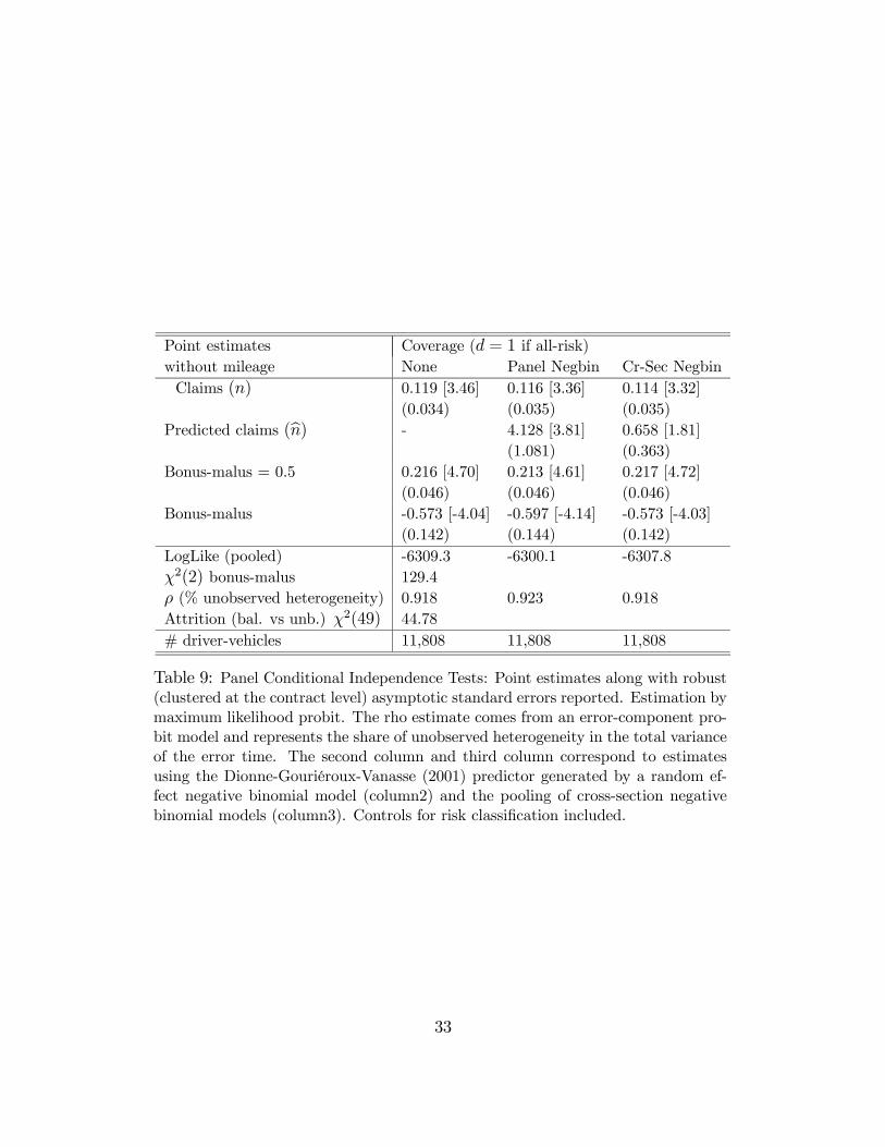
The risk classification parameters remain relatively stable across years. A Chi-square testfor the restriction that parameters should remain stable across years in a pooled probitwith errors clustered at the contract level yields a value of 104.2 and a p-value of 0.182.We can therefore impose this parametric restriction and pursue a panel data analysiswith invariant parameters. As pointed out in Arulampalam (1999), the parameters inpooled and error component probits (random effect) have a direct correspondence butthe error component probit allows us to identify the share of unobserved heterogeneityin the total variance of the error term.13 If there exist contract-specific attributes thatare constant over time but independent of observable risk classification, this will leadto serial correlation across years. Enforcing parameter restrictions across time and alsoallowing for serial correlation in this way can improve the efficiency of the estimator. Weperform the Dionne, Gouriéroux, and Vanasse (2001) first-step estimate using a negativebinomial model with beta random effects in the dispersion parameter14 (Hausman et al.,1984). We also make predictions from the cross-sectional negative binomial estimates.Table 9 reports the pooled probit estimates for the Dionne, Gouriéroux, and Vanasse test(including the bonus-malus coefficient), along with the share of unobserved heterogeneityin contract choice from the error component probit.

[Table 9 about here]13Define udit = αdi + εdit such that if αdi and εdit are independent of each other and normally

distributed with variances σ2ε and σ2α, we will obtain that the pooled probit estimates of πn will beπn/

p(σ2ε + σ2α) while the error component probit estimate will be πn/σε. Therefore, one must multiply

the error component probit estimate byp(1− ρ) where ρ = σ2α/(σ

2ε+σ2α) in order to get pooled probit

estimates.14The negative binomial random effect model allows δ, the overdispersion parameter, to vary across

contracts by assuming that it follows a beta distribution.

15

We obtain a sufficient increase in precision, with no significant variation in the size ofparameters. We can easily reject the conditional independence assumption and concludefor some evidence of residual asymmetric information. However, we do not know thesource of this correlation, whether it is adverse selection or moral hazard.Since the attrition rate in the panel is high, we first verify if those leaving have a

different conditional relationship between claims and contract choice. Those leaving thepanel in a particular year may possibly be those who are faced with increasing premiums.In this case, these should be the contracts most probably scheduled for revision of termsin the last observed year. Consequently, there should be a stronger association betweenclaims and contract choice for these contracts than for those remaining in the panel. Wetest this idea by comparing estimates from the unbalanced sample containing those wholeave and remain and the balanced sample containing only those who remain. Underthe null of attrition that does not bias the inference supporting the relationship betweencontract choice and claims, the estimator bθu, for the unbalanced sample, should beasymptotically efficient while bθb , the balanced sample estimator, should not be efficientfor all parameters in the conditional independence test (see Nijman and Verbeek, 1996):V ar(bθb − bθu) = V ar(bθb) − V ar(bθu) . We can use the Durbin-Wu-Hausman test (seeHausman, 1978) that should be Chi-square distributed with degrees of freedom dim(θ)

under the null of H0 : bθb−bθu = 0.15 Under non-random attrition these estimates shoulddiffer considerably. The test applied to the specification in column 1 of Table 9 yieldsa value of 44.78 which has a p-value of 0.644. It thus finds no evidence of an attritionbias. Note that, as this test may not be powerful enough, we also rely on another testproposed by Fitzgerald et al. (2000) to check for the possibility of a bias due to attrition.If the probability of attrition depends on past accidents and past contract choices, thenwhether or not a contract exits or remains in the panel should be correlated with initialcontract choice and initial claims. We can estimate the following model

di1 = I(x0i1βd + πnni1 + πaai + πanni1ai + udi1 > 0)

where ai = I(Ti < 3) and Ti is the number of years in which a contract is observed.The null hypothesis should therefore be that where both πan and πa are zero. This testperformed on the specification used in the first column of Table 9 yields the followingrelationship (t-values in brackets):

di1 = I(...+ 0.196[1.45]

ni1 − 0.055[−0.93]

ai − 0.042[0.30]

ni1ai + udi1 > 0)

N = 11, 808; χ2(2) = 1.26

This test leads to a conclusion similar to that of the Durbin-Wu-Hausman test. Thereappears to be no evidence of an attrition bias. Indeed, with a survey of policyholders,15The test statistic is W = (bθb − bθu)0V ar(bθb − bθu)−1(bθb − bθu).

16

attrition is presumably much less problematic than when using data from insurers wherea change in contract parameters may lead policyholders to switch insurer. Furthermore,with the conditional independence test which controls for a long list of characteristicswe are less likely to face the risk of retention based on unobservables.

4.4 Summary of Conditional Independence Tests

Results from this section can be summarized as follows: Experience rating plays a con-founding role in our attempts to study the conditional correlation between contractchoice and claims. Once we focus on the bonus-malus coefficient, a clearer positive cor-relation emerges, pointing to the presence of asymmetric information. The rejection ofconditional independence is not due to false specification of the conditional mean of therisk classification equation. Longitudinal data are of considerable help in improving theprecision of the estimates. Finally, we find no evidence of any attrition bias.We now investigate the dynamic link between contract choice and claims, taking into

account experience rating, in order to design a test that will distinguish between adverseselection and moral hazard.

5 Adverse Selection and Moral Hazard

Let us start with the conditional independence test in (1)

H0 : F (di|xi, ni; θd) = F (di|xi; θd).

Using the law of joint probabilities F (di|xi; θd) = F (di,ni|xi;θ)F (ni|xi;θn) , we can write H0 in an

equivalent formH0 : F (di, ni|xi; θ) = F (di|xi; θd)F (ni|xi; θn)

where θ, θn and θd are some finite-dimensional parameter vectors.Indeed, as Chiappori and Salanié (2000) note, we can perform such a test by formu-

lating a bivariate probit of the form

ni = I(x0iβn + uni > 0) (3)

di = I(x0iβd + udi > 0).

The test focuses on the correlation between uni and udi denoted by ρu. The test forconditional independence becomes H0 : ρu = 0. Now, let us consider the case where we

17

have Ti repeated observations on a contract (assume Ti = T fixed for simplicity). Wecan decompose the error term of both equations in (3) into an error component structure

uni = αni + εnit

udi = αdi + εdit.

Assume, for a moment, that the econometrician and both contractual parties canobserve the pair αi = (αni,αdi) where αni may represent specific policyholder character-istics, while αdi could represent specific contract characteristics. The test for asymmetricinformation now takes the form

H0 : F (dit, nit|xit,αi; θ) = F (dit|xit,αit; θd)F (nit|xit,αit; θn) ∀t.

Hence, if we again assume normality for (εdit, εnit) we still have a test for residualcontemporary asymmetric information given by testing ρε = 0. Now include the historyof each of the decision variables in the conditioning set such that

H0 : F (dit, nit|xit, dit−1, nit−1,αi; θ) =F (dit|xit, dit−1, nit−1,αi; θd)F (nit|xit, dit−1, nit−1,αi; θn) ∀t > 1.

This still yields a test for residual asymmetric information given by ρε = 0. Lookingat the marginals, we claim that the cross-sectional variation in contract choice dit−1,holdingαi and nit−1 constant, effectively identifies moral hazard if nit responds positivelyto such a variation. Under pure adverse selection, such variation in contract choicewill not lead to a subsequent change in the distribution of claims in the next period.Therefore, we propose to test for the presence of moral hazard by using Granger causality,crucially holding αi fixed (Chamberlain, 1984): Rejecting the following null hypothesis,

H0 : F (nit|xit, dit−1, nit−1,αi; θn) = F (nit|xit, nit−1,αi; θn) ∀t > 1 (4)

will lead us to conclude that there is evidence of dynamic moral hazard.One can distinguish moral hazard from adverse selection within this dynamic frame-

work because changes in exogenous risk factors (adverse selection) are controlled overtime. So access to longitudinal data is crucial. Since we do not observe αi and thecross-sectional variation in dit−1, nit−1, is, by construction, correlated with unobservedheterogeneity, one additional observation is therefore needed in order to have two pairsof (nit, dit) and (dit−1, nit−1) from which we can separate the effect of unobserved hetero-geneity. This is analogous to the identification argument Heckman (1981) makes for adynamic binary-choice model with an error-component structure. Two remarks shouldbe made at this point.

18

First, we must address the possibility that dit responds to nit+1 and, similarly,that nit responds to dit+1 .This is a classical difficulty in applying Granger causality,as the test would reveal the wrong causal mechanisms.16 If one variable responds toits lead instead of the other variable responding to the lag, then causality is reversed.However, we would argue that this concern does not apply for testing moral hazard inthe presence of experience rating in France, because of the particular features of thelong-term contractual relationship existing here.Indeed, this market has been described as one which is characterized by semi-

commitment, because it offers the possibility of renegotiation and switching insurer.The partial commitment from the part of the insureds implies that there is little incen-tive for them to choose contracts based on the evolution of future accident outcomespassed the date when the contract ends (one year) even if they have rational expecta-tions about accidents. Since they are free to renegotiate the contract without cost thefollowing year, we can claim that the choice of insurance coverage is not based on claimsforecast two years in advance. We would therefore argue that the Granger causality testfrom d to n will indeed serve to detect moral hazard.The second remark concerns the test for residual instantaneous asymmetric informa-

tion. Even with our use of longitudinal data, the point Chiappori (2000) made concern-ing the impossibility of separating moral hazard and adverse selection instanteneouslyis still valid. It is indeed possible that contract change will, in the very short term,affect the probability of a claim such that there could be contemporaneous causalityfrom contract choice to claims and vice versa. This is due to the discrete-time natureof the data we use. Time cannot serve as a “pseudo-instrument” to identify causalityand one would need external instruments to distinguish one from the other, which mayprove very difficult.17 Therefore the contemporaneous test (ρε) is still one for residualasymmetric information, although the dynamic moral hazard test does distinguish moralhazard from adverse selection.

5.1 Parametric Model and Initial Conditions

As we have seen in Table 4, very few annual contracts feature more than one claim.Therefore, with some abuse of notation, we will define nit as the occurrence of at leastone claim. We postulate the following parametric model for the evolution of claims and16See Hamilton (1994, 306-309) for an example where the wrong conclusion about causality is drawn

from a Granger causality test in the presence of rational expectations.17Because of the discrete choice nature of both variables of interest, there would be an additional

“coherency” problem if both simultaneous effects were present. Coherency is defined as the impossibilityof finding a unique mapping from (εdit, εnit) to the data for any given value of the parameters. Thesimultaneous binary-choice model suffers from this problem as emphasized by Schmidt (1980).

19

contract choice:

dit = I(x0itβd +w0itγd + φdddit−1 + φdnnit−1 + αdi + εdit > 0), (5)

nit = I(x0itβn +w0itγn + φnnnit−1 + φnddit−1 + αni + εnit > 0).

i = 1, ..., N, t = 1, .., Ti.

We definewit to be a set of variables that are predetermined at t such thatE(εditwit+s) =0 and E(εnitwit+s) = 0 are assumed to hold for s = 0 but may not necessarily hold fors > 1. This plausibly allows for feedback from accidents and contract choice to certainvariables such as the bonus-malus and lags in the vehicle’s mileage. The bonus-maluscoefficient has proved to be of particular importance in the conditional independencetests. Therefore, wit is of the same nature as lags of the dependent variables, given thatwit may also possibly be correlated with unobserved heterogeneity (αni,αdi).The dynamic test for moral hazard is one for

H0 : φnd ≤ 0 (6)

H1 : φnd > 0

while the contemporaneous test for residual asymmetric information (plausibly againmoral hazard or adverse selection) is given by

H0 : ρε ≤ 0 (7)

H1 : ρε > 0

For a small panel (small T ), predetermining a dynamic binary choice with an error-component structure will lead to the initial condition problem (Heckman, 1981). Since(αni,αdi) are unobserved we must somehow integrate out unobserved heterogeneity fromthe conditional probabilities. Because contracts have a prior history which is hidden forthe econometrician, we need to sort out the joint density of (αni,αdi) and the priorinitial conditions, since di0 and ni0 are missing. Indeed, we need to know how thedifferent (αni,αdi) got sorted out in different outcomes, since it is unlikely to be random.We follow the solution proposed by Wooldridge (2000) and assume the mean of thedistribution of (αni,αdi) to be a linear index y0i1ζd and y

0i1ζn of endogenous variables

and predetermined variables, yi1 = (di1, ni1,wi1)0.18 The parameters ζn and ζd do

not capture causal effects and therefore cannot be used to test any of the relevantsources of asymmetric information. They capture both the correlation in unobservedheterogeneity and the effect of past causal mechanisms, such as the moral hazard prior18Replacing unobserved heterogeneity by their conditional means yields the following equations re-

20

to the observation period. One can note that we do ”lose” one observation in the process.This is a good illustration of the identification issue. Unobserved heterogeneity entailsthe use of two repeated observations, conditional on unobserved heterogeneity and recenthistory of the variables, in order to test for moral hazard.

5.2 Estimation

If the conditional expectations in (5) were linear in parameters, the two equations couldbe estimated separately using ordinary least square, as they contain the same condi-tioning variables. In essence, this is a reduced-form vector autoregression. However,since the two equations are non-linear because of the binary nature of the dependentvariables, we estimate them jointly using a bivariate probit with correlated errors. Notethat normality was not rejected in the conditional independence tests. Furthermore, weallow the errors εnit, εdit to be clustered at the contract level. Finally, we use the sameset of conditioning variables as in the conditional independence tests, as these are crucialfor the contemporaneous test of asymmetric information. We replace (αni,αdi) by theirconditional expectations to take account of initial conditions and take the bonus-malusand mileage to be the predetermined variables in wi1. Including mileage in lags did notprovide any changes in the results and yielded statistically insignificant parameters.Quite naturally, we use the unbalanced panel, although the identification of moral

hazard will come primarily from the contracts observed over three years (1049). Theaddition of those exiting or entering during the three years (but remaining for 2 years)may improve the efficiency of the estimator. Trivially, those remaining in the panel foronly one year will not be used because of the presence of lagged decisions in the twoequations.

5.3 Results

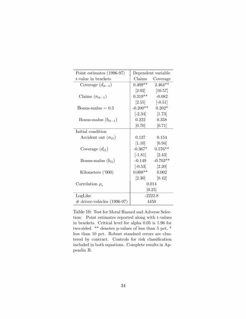
Estimation results are presented in Table 10. (Complete results are in Appendix B.)


placing (5),

dit = I(x0itβd +w0itγd + φdddit−1 + φdnnit−1 + y

0i1ζd + εdit > 0), (8)

nit = I(x0itβn +w0itγn + φnnnit−1 + φnddit−1 + y

0i1ζn + εnit > 0).

i = 1, ...,N, t = 2, .., Ti.

21

We find evidence that the rejection of conditional independence is entirely derivedfrom the presence of moral hazard in the contractual relationships that we observe. Thehypothesis of no moral hazard is rejected at the 5% level (t-value=2.02).19 Indeed, wefind that those switching from all-risk coverage to third-party coverage tend to exhibita 5.9 percentage point decrease in the probability that they will file a claim the nextyear. Therefore, these policyholders try harder to avoid claims when faced with higherprospective insurance premia.This change of insurance coverage can itself be triggered by the rising expected cost

of accidents under an all-risk insurance policy. Indeed, those moving from a maximalbonus of 0.5 because of an at-fault claim in the last year have a 5.8% higher probabilityof switching from all-risk coverage to third-party coverage. This effect is significant ata level of 10% (t-value = 1.73). This can be explained by rising premiums not only dueto a posteriori pricing but potentially also due to a priori pricing, as many suspect.Initial conditions also reveal the sorting of contracts along bonus-malus coefficient linesin initial-year contracts. Those with high bonus-malus coefficients tend to opt for third-party insurance policies (t-value = 2.20) and also file fewer claims (not significant at10%).The second test we proposed is designed to capture residual contemporaneous asym-

metric information. We do not find evidence of residual asymmetric information whenlooking at the correlation parameter between error terms. This coefficient is low (0.014)and imprecisely estimated (t-value = 0.25). It is very similar to the one found by Chiap-pori and Salanié (2000) who were careful to isolate adverse selection from moral hazardby selecting a sample of drivers who are less likely to be affected by moral hazard. Thetest we did in this paper effectively creates a similar setting by using longitudinal data toreplicate conditions in which “moral hazard” stemming from past relationships amongcontractual relationships is taken into account.One last interesting result is that we find evidence of a positive contagion effect

(positive state-dependence) in the claim process, which we can distinguish from thecontagion effect created by unobserved heterogeneity in claims. A policyholder filing aclaim in a given year is 6.1% point more likely to file another claim in the next yearas compared to another policyholder with a comparable risk profile (both observed andunobserved) who did not file a claim (t-value = 2.55). As suggested by Abbring et al.(2003a) not finding a net negative contagion effect does not necessarily imply that moralhazard is absent under experience rating. Note that, in testing for such an effect, wecontrol for initial exposure to risk by including mileage among the initial conditions.19Strictly speaking according to the test in (6), the one sided p-value is 0.021.

22

6 Conclusion

Testing for residual asymmetric information in different markets is becoming a significantresearch topic (Dionne and St-Michel, 1991; Fortin and Lanoie, 1992; Genesove, 1993;Hendel and Lizzeri, 1999; Crocker and Tennyson, 2002; and many others, Chiappori andSalanié, 2003). The main objective is to verify whether actual stylized contracts derivedfrom the theory deal efficiently with different information problems. A more difficulttask is to identify the nature of the different information asymmetries. Researchersusually face an identification problem because the same prediction or correlation maycorrespond to either ex-ante moral hazard, ex-post moral hazard, or adverse selection insingle period contracting.20

To overcome this identification problem, Chiappori (2000) has suggested the use ofmulti-period data. Multi-period data seems to be a necessary but not sufficient condi-tion. Indeed, focusing on claims dynamics, Abbring et al. (2003a, 2003b) were not ableto identify any form of moral hazard in the data set obtained from a French insurer. Inthis research, we used a unique longitudinal survey of policyholders in France to takeexperience rating into account. Indeed, we had access to the dynamic claims as wellas the dynamic contract choices of the policyholders. Having access to contract choicesincreased the number of instruments available to isolate moral hazard from adverse selec-tion. We were able to apply the Granger causality test controlling for the unobservables(Chamberlain, 1984).Our results indicate, first, that residual asymmetric information is present in our

panel. They also isolate dynamic moral hazard: drivers faced with significant increasesin their bonus-malus and premium switch from all-risk coverage to third-party coverageonly (partial insurance) and, improving their safe-driving efforts, significantly reducetheir chances of having an accident in the next period.Our results also indicate that there is no residual contemporaneous asymmetrical

information in the data, when the above dynamic behavior is isolated, confirming theresults of Chiappori and Salanié (2000) and Dionne et al. (2001), who did not haveaccess to multi-period contracts.The presence of a bonus-malus scheme was crucial to the derivation of our results.

But our results also justify this scheme existence by crediting its introduction for ap-propriate incentives for road safety. More research on its optimal form or on (improved)substitutes seems needed to respond to the criticisms directed against it over the last tenyears. It is not clearly apparent also that the industry’s actual form of commitment tothe bonus-malus scheme in France reduces competition among insurers. This issue is im-20For an analysis of ex-post moral hazard along with ex-ante moral hazard and adverse selection, see

Dionne and Gagné (2002).

23

portant because, as shown by Chiappori et al. (2004), market power can itself partiallyexplain contemporaneous residual correlation between claims and insurance coverage.

References

[1] J.H. Abbring, P.A. Chiappori, and J. Pinquet (2003a): “Moral Hazard and DynamicInsurance Data,” Journal of the European Economic Association 1, 767-820.

[2] J.H. Abbring, P.A. Chiappori, J.J. Heckman, and J. Pinquet (2003b): “AdverseSelection and Moral Hazard in Insurance: Can Dynamic Data Help to Distinguish?”Journal of the European Economic Association 1 (Papers and Proceedings), 512-521.

[3] W. Arulampalam (1999): “A Note on Estimated Coefficients in Random EffectsProbit Models,” Oxford Bulletin of Economics and Statistics 61, 4, 597-602.

[4] Council of the European Communities (1992), directive No 92/49/CEE “Thirddirective, insurance not life,” OPEC, European Commission, Brussels.

[5] G. Chamberlain (1984): “Panel Data,” in Handbook of Econometrics, vol 2, chapter22, Zvi Griliches and Michael D. Intriligator (eds), Elsevier Science.

[6] A. Chesher and M. Irish (1987): “Residual Analysis in the Grouped and CensoredNormal Linear Model,” Journal of Econometrics 34, 1, 33-61.

[7] P.A. Chiappori (2000): “Econometric Models of Insurance Under Asymmetric Infor-mation,” in Handbook of Insurance, G. Dionne (ed.), Kluwer Academic Publishers,363-392.

[8] P.A. Chiappori and B. Salanié (2000): “Testing for Asymmetric Information inInsurance Markets,” Journal of Political Economy 108, 1, 56-78.

[9] P.A. Chiappori and B. Salanié (2003): “Testing Contract Theory: A Survey of SomeRecent Work,” in Advances in Economics and Econometrics - Theory and Applica-tions, Eighth World Congress, Volume 1, M. Dewatripont et al. (eds), EconometricSociety Monographs, 115-149.

[10] P.A. Chiappori, I. Macho, P. Rey, and B. Salanié (1994): “Repeated Moral Hazard:The Role of Memory, Commitment, and the Access to Credit Markets,” EuropeanEconomic Review 38, 1527-1553.

24

[11] P.A. Chiappori, B. Jullien, B. Salanié, and F. Salanié (2004): “Asymmetric Infor-mation in Insurance: General Testable Implications,” Working paper, University ofChicago, CREST, and Université de Toulouse.

[12] K. Crocker and A. Snow (1986): “The Efficiency Effects of Categorical Discrimina-tion in the Insurance Industry,” Journal of Political Economy 94, 321-344.

[13] K. Crocker and S. Tennyson (2002), “Insurance Fraud and Optimal Claims Settle-ment Strategies,” Journal of Law and Economics 45, 469-507.

[14] M. Dahchour (2002): “Tarification de l’assurance automobile, utilisation du permisà points et incitation à la sécurité routière : une analyse empirique,” Ph. D thesis,University of Paris X-Nanterre, France.

[15] G. Dionne (2001): “Insurance Regulation in Other Industrial Countries,” in Dereg-ulating Property-Liability Insurance, J. D. Cummins (ed.), AEI-Brookings JointCenter For Regulatory Studies, Washington, 341-396.

[16] G. Dionne and N. Doherty (1994): “Adverse Selection, Commitment and Renego-tiation: Extension to and Evidence from Insurance Markets,” Journal of PoliticalEconomy102, 209-235.

[17] G. Dionne and R. Gagné (2002): “Replacement Cost Endorsement and Oppor-tunistic Fraud in Automobile Insurance,” Journal of Risk and Uncertainty 24, 3,213-230.

[18] G. Dionne and P. St-Michel (1991): “Workers’ Compensation and Moral Hazard,”Review of Economics and Statistics 73,236-244.

[19] G. Dionne, C. Gouriéroux, and C. Vanasse (2001): “Testing for Evidence of AdverseSelection in the Automobile Insurance Market: A Comment,” Journal of PoliticalEconomy 109, 444-453.

[20] J. Fitzgerald, P. Gottschalk, and R. Moffitt (1998): “An Analysis of Sample Attri-tion in Panel Data: The Michigan Panel Study of Income Dynamics,” The Journalof Human Resources 33, 2, 251-299.

[21] N. Fombaron (1997): “Contrats d’assurance dynamiques en présenced’antisélection: les effets d’engagement sur des marchés concurrentiels,” Ph.Dthesis, University Paris X-Nanterre, France.

[22] N. Fombaron (2002): “Dérégulation du bonus-malus en assurance automobile etincitations à la sécurité routière: le cas de la France,” Assurances 69, 4, 589-601.

25

[23] B. Fortin and P. Lanoie (1992): “Substitution Between Unemployment Insuranceand Workers’ Compensation,” Journal of Public Economics 49, 287-312.

[24] D. Genesove (1993): “Adverse Selection in the Wholesale Used Car Market,” Jour-nal of Political Economy 101, 644-665.

[25] C. Gouriéroux, A. Monfort, and A. Trognon (1984): “Pseudo Maximum LikelihoodMethods: Application to Poisson Models,” Econometrica 52, 701-720.

[26] C. Granger (1969): “Investigating Causal Relations by Econometric Models andCross-spectral Methods,” Econometrica 37, 3, 424-438.

[27] J. Hausman, H. Hall, and Z. Giriliches (1984): “Econometric Models for CountData with an Application to the Patents-R&D Relationship,” Econometrica 52,909-938.

[28] J.J. Heckman (1981): “The Incidental Parameters Problem and the Problem of Ini-tial Condition in Estimating a Discrete-Time Data Stochastic Process”, in Struc-tural Analysis of Discrete Data with Econometric Applications, C.F. Manski and D.McFadden (eds.), MIT Press, Cambridge, 179-195.

[29] I. Hendel and A. Lizzeri (2003): “The Role of Commitment in Dynamic Contracts:Evidence from Life Insurance,” Quarterly Journal of Economics 118, 299-327.

[30] I. Hendel and A. Lizzeri (1999): “Adverse Selection in Durable Goods Markets,”American Economic Review 89, 1097-1115.

[31] H. Kunreuther and M. Pauly (1985): “Market Equilibrium with Private Knowl-edge,” Journal of Public Economics 26, 269-288.

[32] T.E. Nijman and M. Verbeek (1996): “Incomplete Panels and Selection Bias,” inThe Econometrics of Panel Data: Handbook of Theory and Applications (SecondRevised Edition), L. Mátyás and P. Sevestre, (eds.), Kluwer Academic Publishers,Dordrecht, 449-490.

[33] P. Picard (2000): “Les nouveaux enjeux de la régulation des marchés d’assurance,”Working Paper no 2000-53, THEMA, Université Paris X-Nanterre.

[34] J. Pinquet (2000): “Experience Rating through Heterogeneous Models,” in Hand-book of Insurance, G. Dionne (ed.), Kluwer Academic Publishers, Boston.

[35] J. Pinquet (1999): “Une Analyse des Systèmes Bonus-Malus en Assurance-Automobile,” Assurances 67, 2, 241-249.

26

[36] R. Puelz and A. Snow (1994): “Evidence on Adverse Selection : Equilibrium Signal-ing and Cross Subsidization on the Insurance Market,” Journal of Political Economy102, 236-257.

[37] D. Richaudeau (1998): “Le marché de l’assurance automobile en France,” Assur-ances 66, 3, 423- 458.

[38] D. Richaudeau (1999): “Automobile Insurance Contracts and Risk of Accident:an Empirical Test Using French Individual Data,” Geneva Papers on Risk andInsurance Theory 24, 97-114.

[39] G. Rosenwald (2000): “Devenir du bonus-malus,” Communication at La SociétéFrançaise de Statistique , November 29, 2000, Paris.

[40] M. Rothschild and J. Stiglitz (1976): “Equilibrium in Insurance Markets: An Essayon the Economics of Imperfect Information,” Quarterly Journal of Economics 90,630-649.

[41] P. Schmidt (1981): “Constraints on the Parameters in Simultaneous Tobit and Pro-bit Models,” in Structural Analysis of Discrete Data with Econometric Applications,C.F. Manski and D. McFadden (eds.), MIT Press, Cambridge, 422-434.

[42] C. Wilson (1997): “A Model of Insurance Markets with Incomplete Information,”Journal of Economic Theory 16, 167-207.

[43] R. Winter (2000): “Moral Hazard in Insurance Markets,” in Handbook of Insurance,G. Dionne (ed.), Kluwer Academic Publishers, Boston, 155-183.

[44] J.M. Wooldridge (2000): “A Framework for Estimating Dynamic, Unobserved Ef-fects Panel Data Models with Possible Feedback to Future Explanatory Variables,”Economics Letters 68, 245-250.

27

Panel structure Number of driver-vehiclesstatus Year 1995 Year 1996 Year 1997

Enter 5443 3464 2901Exit 3052 3796 -Remain 2391 2059 -Total 5443 5855 4960

Table 1: Composition of the SOFRES Survey: Number ofcontracts observed in each wave. Exit refers to contractsthat will exit the panel at the end of the year while Enterrefers to contracts which enter the panel (first observed)in a given year. 1049 observations remain in the panel forthe full three years.

28

(% and mean) Year 1995 Year 1995Gender (male) 62.9 RegionAge Paris 33.418-24 5.2 North 9.225-34 22.3 East 9.835-44 21.7 South 35.245-54 16.5 West 12.455-64 14.7 Occ. drivers 45.265+ 20.0 Network

Rural 13.3SES Position City 40.6Retired 28.3 Road 46.6Farmer/Artisan 4.3 Vehicle ageManager 8.0 Less 3 yrs 34.3Professional 7.6 3-5 yrs 18.6Teacher 19.4 5-10 yrs 33.4Employee 29.1 More 10 yrs 13.7Student 3.2 Experience (yrs)# vehicles 1st quartile 14one 45.8 Median 24two 45.6 3rd quartile 363 and more 8.5 Mean 25.2

# driver-vehicles 5443

Table 2: Contract Characteristics for 1995.

29

1995 1996 1997Declared accident (%) 12.6 11.8 10.7Undeclared accident (%) 7.8 5.5 5.0Bonus-malus (b) (%)= 0.5 64.9 65.9 68.30.5 < b ≤ 1 33.6 32.9 30.81 < b ≤ 1.25 0.9 0.7 0.5b>1.25 0.6 0.4 0.4

Kilometers (’000) mean 13.75 13.6 13.71st quartile 8 8 73rd quartile 18 17 18

All-risk insurance (%) 69.4 69.9 69.1# driver-vehicles 5443 5855 4960

Table 3: Accidents, Contract Choice and Utilizationof Vehicle over 1995-1997: Percentage with one claimor one undeclared accident given. The kilometers arereported in thousands.

ClaimsCoverage None 1 2 3 4Third-party coverage 91.5 7.4 0.9 0.2 0.1All-risk coverage 86.9 11.2 1.6 0.2 0% of contracts 88.3 10.1 1.4 0.2 0.1

Chi-square test 79.2 (p-value<0.001)

Table 4: Distribution of Claims across Different Typesof Contracts 1995-1997: The tabulations (conditionalrelative frequencies) are made using all observationsacross all years. Similar results emerge for yearly tabu-lations. The Chi-square test measures the distance be-tween estimated frequencies and expected cell frequen-cies under the null hypothesis of independence.

30

Claims Undeclared Bonus-malus Kilometers CoverageClaims -Undeclared -0.01 -Bonus-malus 0.08** 0.08** -Kilometers 0.13** 0.05** 0.12** -Coverage 0.06** -0.01 -0.14** 0.18** -

Table 5: Correlation Patterns among Variables: Bivariate correlations. **indicates p-value<0.05, * p-value<0.10.

Point estimates Coverage (di= 1 if all-risk)probit (robust SE) Year 1995 Year 1996 Year 1997With mileageClaims (ni) 0.080 [1.55] 0.107 [1.82] 0.061 [0.90]

(0.052) (0.058) (0.068)LogLike -2123.6 -2258.9 -1919.2Without mileageClaims (ni) 0.089 [1.74] 0.118 [1.99] 0.072 [1.06]

(0.051) (0.054) (0.068)Loglike -2126.7 -2268.7 -1930.1χ2(4) usage (km) 6.22 19.6** 21.8**# driver-vehicles 5443 5855 4960

Table 6: Cross-Sectional Conditional Independence Tests:Point estimates along with robust asymptotic standard errorsreported (in parenthesis) and t-values [in brackets]. Estimationby maximum likelihood probit. Controls for: age dummies (7),experience splines (4), no presence of occasional drivers, prin-cipal network used, number of active drivers, income bracketdummies (9), gender, socio-economic status dummies (8), re-gion (4), age of vehicle splines (4), type of vehicle (5). Mileageis included as 4 splines in thousands of kilometers. The sameset of controls is used in all estimations. Complete results inAppendix A.

31

Point estimates Coverage (d = 1 if all-risk)probit Year 1995 Year 1996 Year 1997Without mileageClaims (n) 0.084 [1.63] 0.119 [2.01] 0.071 [1.03]

(0.052) (0.059) (0.068)Predicted claims (bn) 2.307 1.793 1.569

(1.037) (1.574) (1.443)LogLike -2124.3 -2268.1 -1929.4# driver-vehicles 5443 5855 4960

Table 7: Cross-Sectional Conditional Independence Tests ofDionne, Gouriéroux, and Vanasse (2001): Point estimates alongwith robust asymptotic standard errors reported. Estimation bymaximum likelihood probit.

Point estimates Coverage (d = 1 if all-risk)probit Year 1995 Year 1996 Year 1997Without mileageClaims (n) 0.097 [1.86] 0.147 [2.49] 0.095 [1.40]

(0.052) (0.059) (0.068)Predicted claims (bn) 2.509 [2.39] 1.934 [1.23] 1.913 [1.40]

(1.052) (1.583) (1.426)Bonus-malus = 0.5 0.123 [1.84] 0.277 [4.10] 0.246 [3.28]

(0.067) (0.067) (0.075)Bonus-malus -0.806 [-4.33] -0.422 [-1.94] -0.514 [-1.98]

(0.185) (0.217) (0.259)LogLike -2103.4 -2242.9 -1909.5

χ2(2) bonus-malus 41.8 50.4 39.8# driver-vehicles 5443 5855 4960

Table 8: Cross-Sectional Conditional Independence Tests for thePresence of Asymmetric Information with Control for the Bonus-Malus: Point estimates along with robust asymptotic standard errorsreported. Estimation by maximum likelihood probit.

32

Point estimates Coverage (d = 1 if all-risk)without mileage None Panel Negbin Cr-Sec NegbinClaims (n) 0.119 [3.46] 0.116 [3.36] 0.114 [3.32]

(0.034) (0.035) (0.035)Predicted claims (bn) - 4.128 [3.81] 0.658 [1.81]

(1.081) (0.363)Bonus-malus = 0.5 0.216 [4.70] 0.213 [4.61] 0.217 [4.72]

(0.046) (0.046) (0.046)Bonus-malus -0.573 [-4.04] -0.597 [-4.14] -0.573 [-4.03]

(0.142) (0.144) (0.142)LogLike (pooled) -6309.3 -6300.1 -6307.8χ2(2) bonus-malus 129.4ρ (% unobserved heterogeneity) 0.918 0.923 0.918Attrition (bal. vs unb.) χ2(49) 44.78# driver-vehicles 11,808 11,808 11,808

Table 9: Panel Conditional Independence Tests: Point estimates along with robust(clustered at the contract level) asymptotic standard errors reported. Estimation bymaximum likelihood probit. The rho estimate comes from an error-component pro-bit model and represents the share of unobserved heterogeneity in the total varianceof the error time. The second column and third column correspond to estimatesusing the Dionne-Gouriéroux-Vanasse (2001) predictor generated by a random ef-fect negative binomial model (column2) and the pooling of cross-section negativebinomial models (column3). Controls for risk classification included.

33

Point estimates (1996-97) Dependent variablet-value in brackets Claims CoverageCoverage (dit−1) 0.409** 2.464**

[2.02] [10.57]Claims (nit−1) 0.319** -0.082

[2.55] [-0.51]Bonus-malus = 0.5 -0.200** 0.202*

[-2.34] [1.73]Bonus-malus (bit−1) 0.222 0.358

[0.70] [0.71]Initial conditionAccident out (ni1) 0.137 0.154

[1.10] [0.94]Coverage (di1) -0.367* 0.576**

[-1.81] [2.43]Bonus-malus (bi1) -0.149 -0.703**

[-0.53] [2.20]Kilometers (’000) 0.008** 0.002

[2.30] [0.42]Correlation ρε 0.014

[0.25]LogLike -2222.8# driver-vehicles (1996-97) 4450

Table 10: Test for Moral Hazard and Adverse Selec-tion: Point estimates reported along with t-valuesin brackets. Critical level for alpha 0.05 is 1.96 fortwo-sided. ** denotes p-values of less than 5 pct, *less than 10 pct. Robust standard errors are clus-tered by contract. Controls for risk classificationincluded in both equations. Complete results in Ap-pendix B.

34

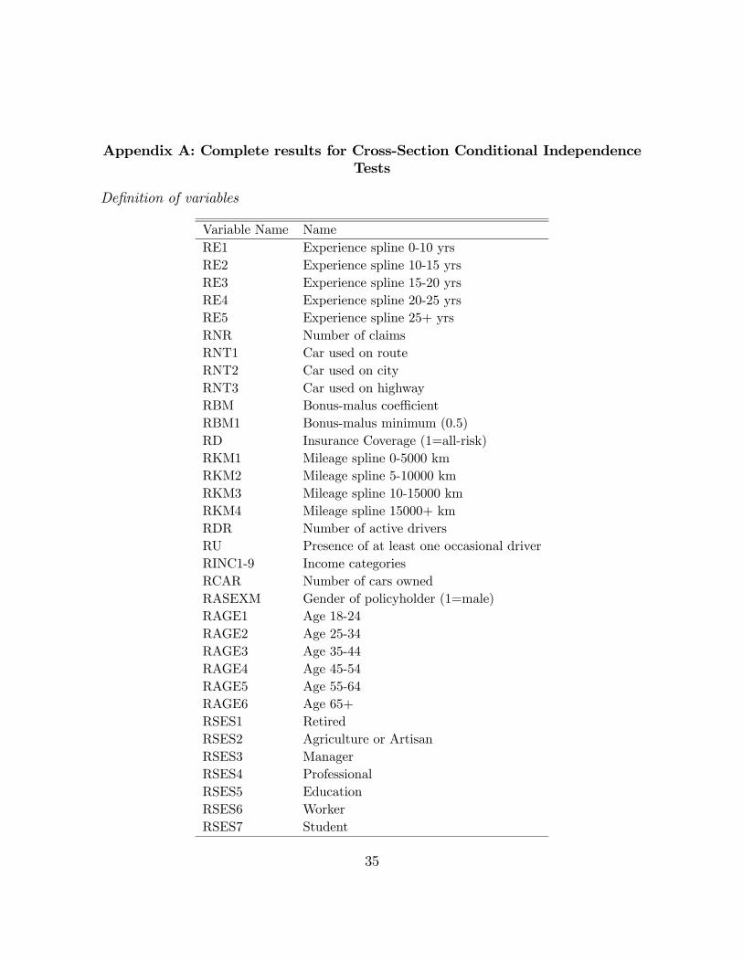
Appendix A: Complete results for Cross-Section Conditional IndependenceTests

Definition of variables

Variable Name NameRE1 Experience spline 0-10 yrsRE2 Experience spline 10-15 yrsRE3 Experience spline 15-20 yrsRE4 Experience spline 20-25 yrsRE5 Experience spline 25+ yrsRNR Number of claimsRNT1 Car used on routeRNT2 Car used on cityRNT3 Car used on highwayRBM Bonus-malus coefficientRBM1 Bonus-malus minimum (0.5)RD Insurance Coverage (1=all-risk)RKM1 Mileage spline 0-5000 kmRKM2 Mileage spline 5-10000 kmRKM3 Mileage spline 10-15000 kmRKM4 Mileage spline 15000+ kmRDR Number of active driversRU Presence of at least one occasional driverRINC1-9 Income categoriesRCAR Number of cars ownedRASEXM Gender of policyholder (1=male)RAGE1 Age 18-24RAGE2 Age 25-34RAGE3 Age 35-44RAGE4 Age 45-54RAGE5 Age 55-64RAGE6 Age 65+RSES1 RetiredRSES2 Agriculture or ArtisanRSES3 ManagerRSES4 ProfessionalRSES5 EducationRSES6 WorkerRSES7 Student

35

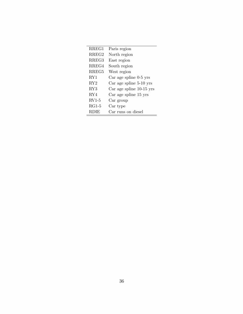
RREG1 Paris regionRREG2 North regionRREG3 East regionRREG4 South regionRREG5 West regionRY1 Car age spline 0-5 yrsRY2 Car age spline 5-10 yrsRY3 Car age spline 10-15 yrsRY4 Car age spline 15 yrsRV1-5 Car groupRG1-5 Car typeRDIE Car runs on diesel

36

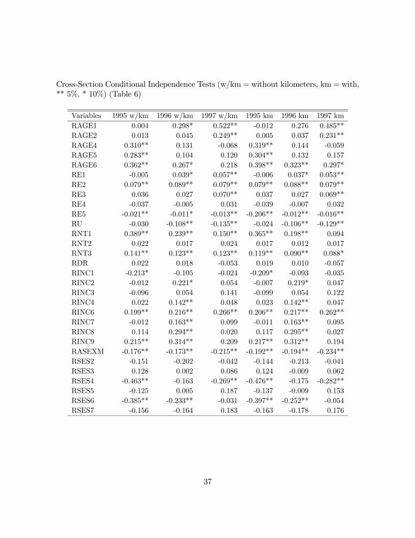
Cross-Section Conditional Independence Tests (w/km = without kilometers, km = with,** 5%, * 10%) (Table 6)

Variables 1995 w/km 1996 w/km 1997 w/km 1995 km 1996 km 1997 kmRAGE1 0.004 0.298* 0.522** -0.012 0.276 0.485**RAGE2 0.013 0.045 0.249** 0.005 0.037 0.231**RAGE4 0.310** 0.131 -0.068 0.319** 0.144 -0.059RAGE5 0.283** 0.104 0.120 0.304** 0.132 0.157RAGE6 0.362** 0.267* 0.218 0.398** 0.323** 0.297*RE1 -0.005 0.039* 0.057** -0.006 0.037* 0.053**RE2 0.079** 0.089** 0.079** 0.079** 0.088** 0.079**RE3 0.036 0.027 0.070** 0.037 0.027 0.069**RE4 -0.037 -0.005 0.031 -0.039 -0.007 0.032RE5 -0.021** -0.011* -0.013** -0.206** -0.012** -0.016**RU -0.030 -0.108** -0.135** -0.024 -0.106** -0.129**RNT1 0.389** 0.239** 0.150** 0.365** 0.198** 0.094RNT2 0.022 0.017 0.024 0.017 0.012 0.017RNT3 0.141** 0.123** 0.123** 0.119** 0.090** 0.088*RDR 0.022 0.018 -0.053 0.019 0.010 -0.057RINC1 -0.213* -0.105 -0.024 -0.209* -0.093 -0.035RINC2 -0.012 0.221* 0.054 -0.007 0.219* 0.047RINC3 -0.096 0.054 0.141 -0.099 0.054 0.122RINC4 0.022 0.142** 0.048 0.023 0.142** 0.047RINC6 0.199** 0.216** 0.266** 0.206** 0.217** 0.262**RINC7 -0.012 0.163** 0.099 -0.011 0.163** 0.095RINC8 0.114 0.294** 0.020 0.117 0.295** 0.027RINC9 0.215** 0.314** 0.209 0.217** 0.312** 0.194RASEXM -0.176** -0.173** -0.215** -0.192** -0.194** -0.234**RSES2 -0.151 -0.202 -0.042 -0.144 -0.213 -0.041RSES3 0.128 0.002 0.086 0.124 -0.009 0.062RSES4 -0.463** -0.163 -0.269** -0.476** -0.175 -0.282**RSES5 -0.125 0.005 0.187 -0.137 -0.009 0.153RSES6 -0.385** -0.233** -0.031 -0.397** -0.252** -0.054RSES7 -0.156 -0.164 0.183 -0.163 -0.178 0.176

37

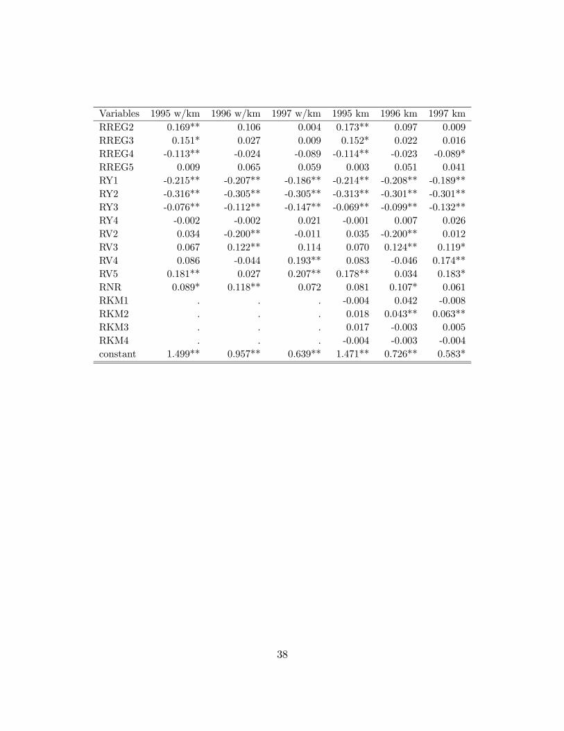
Variables 1995 w/km 1996 w/km 1997 w/km 1995 km 1996 km 1997 kmRREG2 0.169** 0.106 0.004 0.173** 0.097 0.009RREG3 0.151* 0.027 0.009 0.152* 0.022 0.016RREG4 -0.113** -0.024 -0.089 -0.114** -0.023 -0.089*RREG5 0.009 0.065 0.059 0.003 0.051 0.041RY1 -0.215** -0.207** -0.186** -0.214** -0.208** -0.189**RY2 -0.316** -0.305** -0.305** -0.313** -0.301** -0.301**RY3 -0.076** -0.112** -0.147** -0.069** -0.099** -0.132**RY4 -0.002 -0.002 0.021 -0.001 0.007 0.026RV2 0.034 -0.200** -0.011 0.035 -0.200** 0.012RV3 0.067 0.122** 0.114 0.070 0.124** 0.119*RV4 0.086 -0.044 0.193** 0.083 -0.046 0.174**RV5 0.181** 0.027 0.207** 0.178** 0.034 0.183*RNR 0.089* 0.118** 0.072 0.081 0.107* 0.061RKM1 . . . -0.004 0.042 -0.008RKM2 . . . 0.018 0.043** 0.063**RKM3 . . . 0.017 -0.003 0.005RKM4 . . . -0.004 -0.003 -0.004constant 1.499** 0.957** 0.639** 1.471** 0.726** 0.583*

38

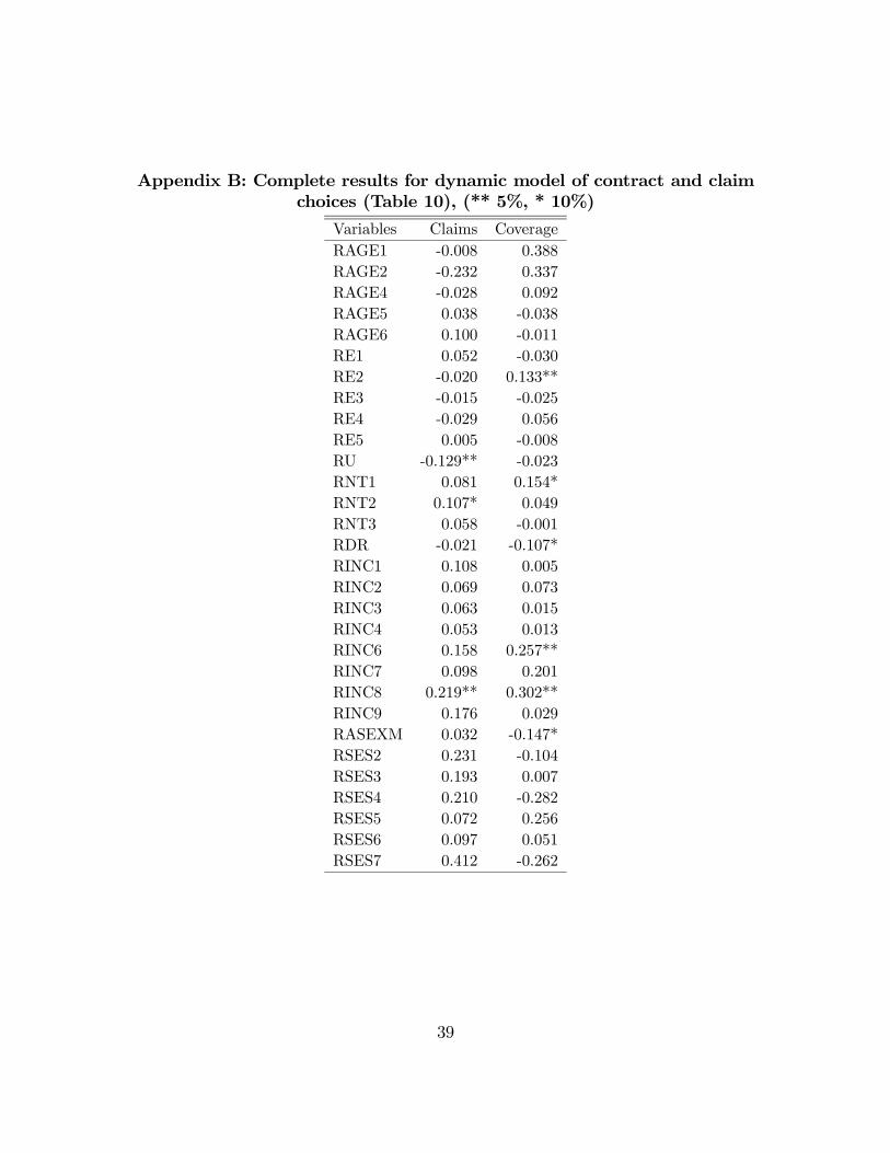
Appendix B: Complete results for dynamic model of contract and claimchoices (Table 10), (** 5%, * 10%)

Variables Claims CoverageRAGE1 -0.008 0.388RAGE2 -0.232 0.337RAGE4 -0.028 0.092RAGE5 0.038 -0.038RAGE6 0.100 -0.011RE1 0.052 -0.030RE2 -0.020 0.133**RE3 -0.015 -0.025RE4 -0.029 0.056RE5 0.005 -0.008RU -0.129** -0.023RNT1 0.081 0.154*RNT2 0.107* 0.049RNT3 0.058 -0.001RDR -0.021 -0.107*RINC1 0.108 0.005RINC2 0.069 0.073RINC3 0.063 0.015RINC4 0.053 0.013RINC6 0.158 0.257**RINC7 0.098 0.201RINC8 0.219** 0.302**RINC9 0.176 0.029RASEXM 0.032 -0.147*RSES2 0.231 -0.104RSES3 0.193 0.007RSES4 0.210 -0.282RSES5 0.072 0.256RSES6 0.097 0.051RSES7 0.412 -0.262

39

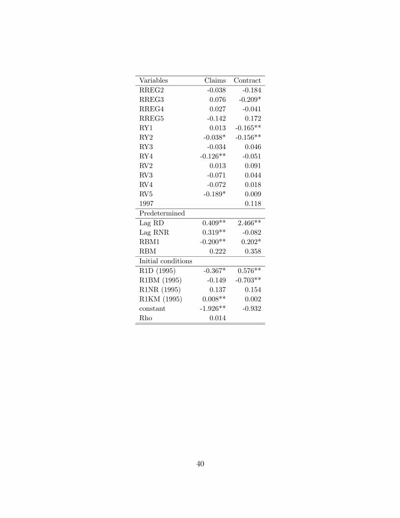
Variables Claims ContractRREG2 -0.038 -0.184RREG3 0.076 -0.209*RREG4 0.027 -0.041RREG5 -0.142 0.172RY1 0.013 -0.165**RY2 -0.038* -0.156**RY3 -0.034 0.046RY4 -0.126** -0.051RV2 0.013 0.091RV3 -0.071 0.044RV4 -0.072 0.018RV5 -0.189* 0.0091997 0.118PredeterminedLag RD 0.409** 2.466**Lag RNR 0.319** -0.082RBM1 -0.200** 0.202*RBM 0.222 0.358Initial conditionsR1D (1995) -0.367* 0.576**R1BM (1995) -0.149 -0.703**R1NR (1995) 0.137 0.154R1KM (1995) 0.008** 0.002constant -1.926** -0.932Rho 0.014

40

separating moral hazard from adverse selection in

Documents