Cost Valuation and Tax Design*

By Magne Emhjellen** and Petter Osmundsen***

** Petoro AS

*** University of Stavanger / Norwegian School of Economics and Bus. Adm.

Abstract Oil project assessment using separate cashflow valuation (Laughton and Jacoby, 1993 and Emhjellen, 1999), presume that the present value of the cost cashflow of oil projects can be calculated using a risk free rate. This paper examines whether this practice, at least to a first approximation, is reasonable. More specifically, the paper examines whether wage hours costs and steel prices, as cost factors in the investment cost stream, are systematic risk factors (i.e. have a beta different from zero). The paper also investigates whether oil price as a factor in the revenue stream is a systematic revenue factor. Separate cash flow evaluation has been dis-cussed in relation to petroleum taxation. A petroleum tax commission in Norway stated that tax reductions due to depreciation should separately be discounted by a risk free rate. We discuss the role of partial cash flow discounting in tax design.

** Magne Emhjellen, Petoro AS, Postboks 300 Sentrum 4002 Stavanger , Norway, Email: Magne.Emhjellen@petoro.no *** Petter Osmundsen, University of Stavanger, Department for Industrial Economics and Risk Management, 4036 Stavanger. Email: Petter.Osmundsen@uis.no, Home page: http://www5.uis.no/kompetansekatalog/visCV.aspx?ID=08643&sprak=BOKMAL

2

1. Introduction

In research related to oil project valuation one often makes the

assumption that the present value of the cost cashflow may be

calculated using the risk free rate (Laughton and Jacoby, 1993 and

Emhjellen, 1999). From a Capital Asset Pricing Model (CAPM)

(Sharpe, 1964, Lintner, 1965) point of view this is only permissible

when the uncertain changes in the cost cashflow is not correlated

with the rate of change in the market portfolio.

To examine this, in Secion 2 we test whether two important

cost factors for oil projects, labour costs and steel prices, are

systematic risk factors (i.e. correlated with the value of the market

portfolio). In addition, we examine in Section 3 whether oil prices

represent a systematic revenue factor, and thus whether the CAPM

beta obtained for oil prices supports using a higher required rate of

return when discounting revenues than when discounting costs.

After identifying the main cost variables for the example project,

historical data on the cost variables, as well as historical data on a

proxy for the market portfolio (The Total Index, Oslo Stock

Exchange), are presented. The betas of these cost variables are then

calculated. The data of our analyses is documented in eight tables,

and can be found in our downloadable working paper 2009/16 at the

University of Stavanger.1

1 http://ideas.repec.org/p/hhs/stavef/2009_016.html

3

The results for the period examined show that the oil price

beta is higher than the cost betas and that risk free discounting of the

cost cashflow may be a reasonable approximation until other cost

factors are identified and examined. The results of the paper

therefore support the idea that revenues should be discounted at a

higher rate than costs when calculating the present value of oil

exploration projects. However, uncertainty related to the correct size

of the individual cashflow betas indicates that further research

should be undertaken on the required rate of return of individual

cashflow streams.

The issues of distinct required rates of return for discounting

individual cashflow streams of oil projects have been raised by the

Tax Commission in Norway. In a tax evaluation study they

implicitely propose that the oil companies should change their

valuation method from discounting the aggregate net cashflow

stream to a method where one specific partial cashflow is valued

separately, namely the tax reduction cash flow from tax depreciation

(Government Report NOU 2000:18).2 The companies’ actual

investment valuation methods are essential to evaluate the

implications of the suggested tax changes. The Commission

recommended a slower pace of tax depreciation. Tax depreciation

time should expand from the current 6 years (linear depreciation) to

2 This deviates from previous tax theory and policy recommendations, see e.g.

Osmundsen (1999a).

4

a time frame more accurately reflecting the economic life of

extraction and transportation installations.3

The companies argued that, with their global practise of

using average discount rates, this would cause considerable tax

increases and lead to a non-neutral tax system that would generate

underinvestment. At any rate, they said, tax reduction cash flows are

by experience not certain, as verified for example by the

Commission’s own report - that proposed tax increases. The Tax

Commission, on the other hand, argued that the revised tax system

would be neutral if the companies correctly discounted tax

reductions by a risk free rate.

This debate raises important questions. Present tax theory

usually presumes average discount rates. In the event of the adoption

of separate cashflow discounting, how should the tax reductions of

depreciations be discounted?

Separate cashflow betas are discussed and estimated in

sections 2 and 3. Uncertainty related to tax recovery and

government tax changes are discussed in Section 4, and in section 5

an example project valuation is shown using the standard net

cashflow discounting method and a separate cashflow discounting

method. Our data sources are presented in an Appendix.

3 The short depreciation time, together with an added depreciation of 30 per cent (uplift), were designed so that the special resource rent tax of 50 per cent should actually only be levied on excess returns, and so that the tax system would not distort investment decisions of the oil companies (neutrality), see White Paper Ot.prp. 1991-92.

5

2. CAPM and separate cashflow betas

Finance theory (Sharpe 1964, Lewellen 1977) related to valuation in

the mean-variance framework argues that in order to calculate the

present value of an uncertain individual cashflow stream one needs

an estimate of the expected value of the cashflow stream and the

cashflow streams covariance with the return of the market portfolio.

The issue of estimating the expected value is raised in section 3. We

now turn to the issue of the required rate of return. The Capital Asset

Pricing Model (CAPM) (Sharpe 1964) relationships states that:

( ) ( )( fmifi RRERRE )−β+= , (2.1)

where E(Ri) is the expected required rate of return on equity of an

asset i and Rf if the risk free rate, E(Rm) is the expected return on the

market portfolio and iβ is the covariance of the return of asset i

with the return of the market portfolio divided by the variance of the

return of the market portfolio ()(

),(

m

mii rVar

rrKov=β ).

From the value additivity principle (Shall, 1972), the net present

value of an asset is the sum of the present values of the component

cashflows of the asset:

∑=

=iM

1jiji XV , (2.2)

6

where Xij is the present value of the jth component of the cashflow

of asset i discounted using the expected required rate of return of the

jth component of asset i, E(Rij), and Mi is the number of cashflow

components of asset i. The expected rate of return on equity of an

asset is equal to the sum of the value weighted expected rates of re-

turn of the individual component cashflows

( ) (∑=

=iM

1jijiji REwRE ) . (2.3)

In equation 2.3, i

ijij V

Xw = and ∑ . From the CAPM rela-

tionship, the expected required rate of return of the jth component of

the cashflow of asset i may be written:

=

=iM

1jij 1w

( ) [ ]fmijfij RRERRE −+= )(β . (2.4)

Substituting equation 2.4 into equation 2.3, βi may be written as

∑=

β=βiM

1jijiji w . (2.5)

An example is where there are only two distinct cashflows generated

by an asset (Lewellen, 1977 and Emhjellen and Alaouze, 2002): the

7

expected after tax revenue cashflow and the expected after tax cost

cashflow, where each of the expected after tax cashflow streams has

a different beta. Thus, j=1,2, and to specify notation, let iDi ββ =1 be

the expected after tax revenue cashflow beta for asset i and

iCi ββ =2 be the expected after tax cost cashflow beta for asset i.

The value of a project given by 2.3 may be written as

C

iD

ii VVV += . (2.6)

In equation 2.6, denotes the PV of the expected after tax reve-

nue cashflow of asset i, and denotes the PV of the expected

after tax cost cashflow of asset i. The beta for asset i may be written

as

DiV

0VCi ≤

CCiD

Dii ww β+β=β , (2.7)

where Ci

Di

DiD

i VVV

w+

= and Ci

Di

CiC

i VVV

w+

= ,

This shows that if an individual cashflow valuation method is to be

used, an integral part in order for the value of the project to be de-

termined, must be to determine the cost cashflow beta and its rela-

tive weight. In other words the systematic risk associated with the

project cost must be determined in order to estimate the required rate

of return and thereby calculate the present value of this cost cash-

flow. An interesting point noted by Lewellen, 1977 is that a higher

8

beta for the capital expenditure cost cashflow implies a higher pro-

ject value. The reason for this is that cost cashflow is a cash outflow

where higher discounting (higher beta implies higher required rate of

return) implies a lower present value of cost. This is contrary to what

is true for revenue, where higher systematic risk implies less value.

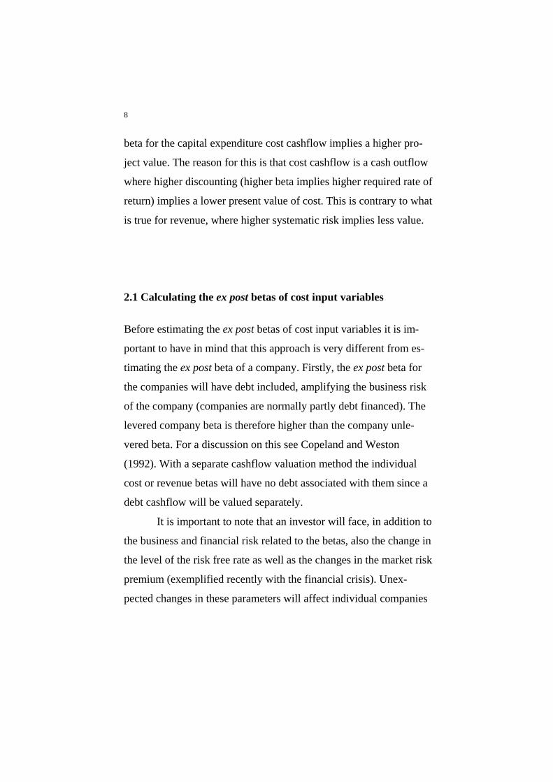
2.1 Calculating the ex post betas of cost input variables

Before estimating the ex post betas of cost input variables it is im-

portant to have in mind that this approach is very different from es-

timating the ex post beta of a company. Firstly, the ex post beta for

the companies will have debt included, amplifying the business risk

of the company (companies are normally partly debt financed). The

levered company beta is therefore higher than the company unle-

vered beta. For a discussion on this see Copeland and Weston

(1992). With a separate cashflow valuation method the individual

cost or revenue betas will have no debt associated with them since a

debt cashflow will be valued separately.

It is important to note that an investor will face, in addition to

the business and financial risk related to the betas, also the change in

the level of the risk free rate as well as the changes in the market risk

premium (exemplified recently with the financial crisis). Unex-

pected changes in these parameters will affect individual companies

9

differently because of different debt levels and different levels of

business risk (i.e. the size of unlevered beta).

A final point regarding estimation of individual cashflow be-

tas is that they will be dependant on the parameters chosen, the total

period and the return period chosen and the market portfolio proxy

(index). In addition, one runs the risk that the returns on the parame-

ters chosen are correlated or that there are parameters not selected

that have various degrees of correlation with the chosen parameters

or the proxy for the market portfolio. However, the company beta is

given by equation 2.5 where a debt level different from zero would

be associated with a beta of debt. With no debt the company or pro-

ject beta can be described by equation 2.7. The results below are

therefore only one first attempt at identifying whether the chosen pa-

rameters has betas different from zero.

The rate of change of the cost data and the rate of change of the To-

tal Index were calculated using the real quarterly data on wage hour

cost, steel prices and the Total Index. The rate of change data are

shown in Table 5.

The ex post betas of the wage hour costs and steel prices were calcu-

lated using Equation (3.1) and the data in Table 5.

)(

),(2 Rm

RmRiCovi σ

β = . (3.1)

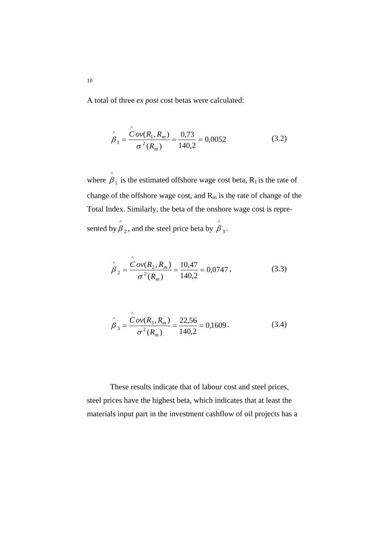
10

A total of three ex post cost betas were calculated:

0052,02,140

73,0)(

),(2

1

^

1

^===

m

m

RRRovC

σβ , (3.2)

where is the estimated offshore wage cost beta, R1

^β 1 is the rate of

change of the offshore wage cost, and Rm is the rate of change of the

Total Index. Similarly, the beta of the onshore wage cost is repre-

sented by , and the steel price beta by . 2

^β 3

^β

0747,02,140

47,10)(

),(2

2

^

2

^===

m

m

RRRovC

σβ , (3.3)

1609,02,140

56,22)(

),(2

3

^

3

^===

m

m

RRRovC

σβ . (3.4)

These results indicate that of labour cost and steel prices,

steel prices have the highest beta, which indicates that at least the

materials input part in the investment cashflow of oil projects has a

11

positive beta.4 Hence, this part of the costs cashflow should be dis-

counted at a rate higher than the risk free rate. For labour cost, al-

though the results show positive betas, the betas (at least for offshore

workhour cost) are only marginally greater than zero.

Using a market risk premium [E(Rm)-Rf] of approximately

6% (Johnsen, 1991), this indicates a required rate of return for the

labour cost portion (with a beta of 0,0747) of approximately 0,44%

above the risk free rate. Similarly, using the steel price beta, the re-

quired rate of return would be approximately 1% above the risk free

rate. A weighted average of labour cost and material cost using these

two betas would therefore indicate a required rate of return less than

1% (0,7%) above the risk free rate.

3. Calculating the ex post oil price beta The oil price beta was calculated using the price data on WTI (West

Texas Intermediate) as given in Standard & Poor’s Platt's Prices and

Data for the period 1986 to 1994. The nominal WTI price data in US

dollars per barrel were converted to real Norwegian currency using

the CPI (Norway) and the NOK/USD exchange rate. The real rate of

change for each period was then calculated quarterly.

4 In deriving the weighted average of the ex post cost betas, we have used their

relative PV weights. Assuming that the PV of the labour cost is 60% of the after tax cost cashflow, and that the PV of steel represents the remaining 40% of the af-ter tax cost cashflow (from the cost structure of project N), the cost cashflow beta is a weighted average of the two cost betas.

12

The data are presented in Table 6. The nominal oil prices in US dol-

lars are shown in column one, the exchange rates in column two, the

CPI in column three, real oil prices in Norwegian currency in col-

umn four, the percentage changes in real oil prices in column five

and the percentage changes in the Total Index in column six.

The oil price beta was calculated in the same manner as the cost be-

tas using the data in Table 1. The oil price beta was calculated to

0,293 using Equation (3.1). This is higher than the cost cashflow be-

tas obtained. It is, however, important to note that the estimated oil

price beta, as the cost betas, could be different with data from differ-

ent time periods and different length of time periods. Thus, the ex

ante oil price beta, just like the cost cashflow beta, may be very dif-

ferent from the calculated ex post beta based on historic data. For the

time period chosen here, however, the oil price beta is substantially

higher than that of the cost cashflow beta, implying that a higher risk

adjustment is called for when discounting the expected after tax rev-

enue stream than when discounting the expected after tax cost

stream. Using this oil price beta as estimate for the required rate of

return on revenues gives a rate 1,8% above the risk free rate (given a

market risk premium of 6%).5

5 It should be noted that the period examined contains the period of the Iraqi invasion of Kuwait where the stock indexes around the world (including the Total Index) depreciated in value while the oil price increased. This has the effect of re-ducing the size of the oil price beta for the period calculated.

13

4. Tax payments and risk adjustment We will raise two issues regarding valuing the tax reduction

cashflow from tax depreciation when valuing cashflows separately.

First, there is the possible direct tax concern for the timing and

likelyhood of cost recovery. Second, there is the issue of possible

government changes in the tax level.

Is it reasonable to discount these tax reductions by a risk free

rate? This is not a trivial issue, since such tax reductions normally

are a non-linear function of both costs and income, where the latter

is crucial for determining whether the oil company is in a tax paying

position. The non-linearity, which may challenge the assumption of

additivity, makes taxes hard to separate from other cash flow

components. Simply discounting with a risk free rate may not be the

relevant approach, due to the option nature of tax payments, see

Lund (1992).

The Norwegian Petroleum Tax Commission makes several

recommendations that would affect the valuation of tax reductions.

In June 2001 the Norwegian Parliament approved an amendment to

the Petroleum Tax Law, allowing the oil companies to carry forward

deficit with interest (risk free rate), and allowing the companies to

transfer losses to other companies.6 Thus, the likelihood of effective

tax deductions are increased, the tax system has become more linear,

6 Transfer of losses at full tax value, however, presumes an efficient market for tax deferrals. In periods of low petroleum prices, there may be a buyer’s market.

14

and the option nature of tax cash flows are less evident than in most

other petroleum tax regimes, e.g., ring fence systems. Another

suggestion from the Petroleum tax Commission, not endorsed by

Parliament, was to increase the tax depreciation time. Such a change

would have increased the political risk for the companies, as there

would be a higher risk risk of a change in tax conditions after

irreversible investments are literally sunk on the seabed. After

investments have been made in facilities that may extract petroleum

for some thirty years, new governments will come into power, and

there is limited possibilities to establish credible guarantees for a

stable tax policy, as one Parliament – according to the Constitution –

cannot commit the tax policies of future Parliaments.

4.1 Tax effects resulting from revenues and costs The norwegian tax base is given by:

Tax base = Revenues (oil price x sale of oil) –operating cost – tax

effect of depreciation –interest cost.

The oil companies will pay a percentage tax of this tax base, making

the tax payments a function of oil price, production and costs.

For revenues, given the assumption that the sale of oil from

an oil project is independent of changes in the value of the market

portfolio, would have a beta equal to the oil price. This follows,

since the after tax revenue is only a scaled down level of the

15

revenues before tax (timing and tax reduction from depreciation

amounts discussed separately). Consequently, the percentage

changes in the after tax cashflow will be equal to the percentage

changes in the before tax cashflow and their correlation with the

changes in the value of the market portfolio will be equal, resulting

in the same beta.

The operating cost cashflow reduces the tax base the same

year while the investment cashflow reduces the tax base through tax

depreciation. Given that the cost betas before tax are only marginally

positive, the cost betas after tax will primarily be linked to the

systematic risk of the oil price. This because the reduction in tax

(after tax cost cashflow) resulting from the cost cashflow will only

be positive when the tax base is positive. In other words, the

negative tax base resulting from low oil prices will have to be

carried forward until the project or company generate a positive tax

base. Consequently, even though the results of this paper indicate

low systematic risk for the cost cashflow (labour cost and steel

prices), the after tax cost cashflow has a timing risk that is the result

of the systematic risk of the oil price. This possible delay of the cost

recovery is a risk that may reduce the full value of the tax reduction

resulting from incurring cost.

4.2 Government changes of tax level

One major uncertainty related to future tax payments is

16

government changes of the tax system which may cause changes in

the tax base or the tax rate. It is likely, given past observations

related to tax changes, that governments are inclined to increase the

tax level when oil prices are stable and high for some time (1-2

years), and to lower the tax level when the oil prices are very low.

One could argue that these tax changes cause the risk to be lower

since over the long run this would reduce the upper levels and

increase the lower levels of the after tax cashflow of the project to

the oil companies, while at the same time providing the same

expected after tax cashflow. However, from past observations, these

changes in tax are sometimes only implemented for new projects

when prices are low (to stimulate new activity), while they are

implemented across the board when prices are high (i.e. a ratchet

effect). Given this type of asymmetric tax policy over the business

cycle, the risk has increased, or rather, the expected value of the

cashflow is reduced by limiting the upside return to the companies

and not limiting the downside.

Consequently, the oil companies will have to take these

possible tax changes into account when calculating project value and

deciding on new oil projects.

17

4.3 Calculating the value of the tax cashflow

Separate cashflow valuation methods require use of correct

required rates of return when discounting the individual after tax

cashflow streams. Given the arguments above the present value of

tax on revenues (and consequently the after tax revenue cashflow)

could be calculated using a required rate of return based on the

before tax beta of revenues.

The present value of the expected after tax cost cashflow

could, like for revenues, be calculated using the estimated required

rate of return on the before tax cost cashflow. However, there

remains the question of how to adjust for the possible delay in time

of cost recovery. As indicated, the risk free rate of interest might not

be enough to fully account for this delay of recovery.

An investigation into oil companies project valuation practise

found that the standard discounted cashflow method was the method

most in use (Siew, 2001). Even though this study does not

distinquish (when asking the energy companies) whether the

discounted cashflow method (DCF) is based on discounting net after

tax cashflow or indvidual cashflows, it is likely that it has been

interpreted by the energy companies as standard net cashflow

valuation. The Value Additivity Principle (Shall, 1972) however,

makes a separate cashflow discounting method possible since the

sum of the individual cashflow values should be equal to the project

value. This however, does not necessarily make this valuation

18

approach a practical method. There remains the issue of whether one

can obtain reasonable estimates for the required rate of return of the

individual cashflow streams. The fact that most energy companies

prefer the DCF based on calculating the present value of the net after

tax cashflow is probably motivated by the difficulies in finding

correct required rates of return for the individual cashflows streams.

This makes further research into separate cashflow valuation

interesting.

5. Oil project valuation example A valuation of an oil project will be illustrated using real oil project

data obtained from Statoil (Project N in Emhjellen, 1999). The

project data are given in Table 7.

5.1 Assumptions used in calculating project NPV

The expected after tax cashflows used in calculating present values

are based on the Norwegian tax regime. The assumptions are as fol-

lows:

1) A 50% special tax is applied to the offshore oil industry. The actual

amount of special tax is determined by the tax base, which is calculated

as follows:

19

Tax base = Revenue (d) - Operating cost (OC) - Depreciation tax shield

(DTS) - Interest payments (IP) - Additional depreciation allowance

(ADA). The special tax is equal to the tax base multiplied by 0.5.

2) An ordinary corporate tax rate of 28% is applied to tax base special tax

less ADA (uplift).

3) Total tax = special tax +ordinary tax

With the separate cashflow discounting method of NPV calculation,

revenue cashflow tax and cost cashflow tax are equal to:

4) Revenue cashflow tax = d × (0.5+0.28).

5) Cost cashflow tax = total tax - revenue cashflow tax.

6) The depreciation amount is 6 year linear depreciation applied to invest-

ment. This tax benefit can be claimed against other offshore oil revenue

of the company (no ring fence on the NCS). When calculating the ex-

pected after tax cost and revenue cashflows, the tax effect of the depre-

ciation amount is treated as a reduction in costs.

7) The additional depreciation allowance (ADA) (applicable to offshore oil

development) is 30% of investment treated as 6 year linear depreciation.

When calculating the expected after tax cost and revenue cashflows the

tax effect of this depreciation amount is treated as a reduction in costs.

8) All calculations are in US dollars

9) Expected nominal cashflows (expected cost and expected revenue) were

calculated assuming a constant expected inflation rate of 2.0%.

10) The nominal risk free rate of return is assumed equal to 6.5%.

20

11) The expected oil price is assumed constant at a real $20US per barrel.

12) The market risk premium (E(Rm)-Rf) is assumed equal to 6%

13) The levered beta for the company is equal to 1 based on Statoil beta level.

Given a debt level of 30% and a marginal tax rate of 78% the unlevered

company beta is equal to 0.914 (assuming Copeland and Weston, 1992.

Pp. 459). This unlevered beta is used as the project beta to reflect busi-

ness risk.

14) The required rate of return for the oil projects is calculated to be nominal

11.98% =12% based on assumption 10, 12 and 13.

5.2 Results

A cashflow model was created using the Excel spreadsheet (version

5.0). Discounting based on one year periods was chosen for the

model because the data are annual. The cashflow results and NPV

calculated using the standard net cashflow discounting method

(396,4 million USD) are shown in Table 8.With separate cashflow

valuation the tax on revenue is the marginal tax rate of 78%. The tax

on the cost cashflow however, may not be calculated independantly

of revenues since the revenues of the project determines when the

costs can be recovered. The tax on cost is then calculated based on

the difference between tax on revenues and tax on the whole project.

Using a discount rate of 8.3% (1.8% above the risk free rate) when

discounting the expeted after tax revenues gives a present value for

expected after tax revenues of 1214 million USD, while using a

21

discount rate of 7.2% (0.7% above the risk free rate) when

discounting the expected after tax cost gives a present value for the

expected after tax cost casflow of 532 million USD. This gives a

project net present value of 682 million, which is 286 million USD

higher than the NPV obtained using the standard net cashflow

discounting method. This example illustrate the large difference in

valuation that might occur when using a separate cashflow valuation

method. In this case it is the lower discounting of the revenues that

gives a high net present value of revenues which is only slightly

offset (compared to the standard net cashflow discounting method)

by the lower discounting of costs.

It is not reasonable to conclude that the separate cashflow method of

NPV gives better NPV estimates than the NPV obtained using the

standard net cashflow discounting method. For the standard net

cashflow discounting method it is a question of how the required

rate of return for the individual project was obtained. For the

separate cashflow discounting method the question is if the ex post

beta estimates obtained for revenues and costs are reasonable

approximations for the ex ante betas. Is the cost risk in wage rates

and steel prices (price risk), for instance, representative for overall

cost risk in the companies? Also, while the project required rate of

return might reflect a risk adjustment for government tax changes

(based on observed market beta for an oil company), it is not likely

that the rates used in discounting the separate cashflows include

such a risk adjustment. These are reasons why the implementation of

22

a separate cashflow valuation method will be difficult without more

reaserch on market data related to the required rates of return of

individual cashflow streams and their components.

6. Summary and further work

The results indicate that the present value of the expected after tax

cost cashflow stream of oil projects in the North Sea should be

calculated using a lower rate than that applied to the expected after

tax revenue stream. The size of the derived cost betas supports the

approximation of using the risk free rate when calculating the

present value of the cost cashflow. However, there are reasons, as

exemplified by the large difference in net present value of the

example project valuation, that further work should be undertaken to

further examine the systematic risk of both the cost and revenue

streams in an oil project. As mentioned, there are several challenges

before a separate cashflow valuation method can be reccommended.

In addition, for both the standard net cashflow valuation

method and the separate cashflow valuation method, there is the

issue of how to estimate the risk adjusted value of the tax effect of

the depreciation amounts when accounting for the possible delay of

the tax reduction.

23

References

Confederation of Norwegian Business and Industry, 1986-1995. Wages and attendance statistics, quarterly. Copeland, T.E. and Weston, J.F. 1992. Financial Theory and Cor-porate Policy: Third Edition, Addison - Wesley. Pp. 457-459. Emhjellen, M. and Alaouze, C. M. 2002 “Project Valuation when There are Two Cashflow Streams”, Energy Economics, Vol. 24, September, pp. 455-467.

Emhjellen, K., Emhjellen, M., Osmundsen, P. 2002. "Investment Cost Estimates and Investment Decisions", Energy Policy, vol. 30, pp. 91-96. Johnsen, T. 1991. "Criteria for Profitable Investments in Oil Explo-rations: A Report to the Department of Oil and Energy", Norwegian School of Business, November Lintner, J. 1965. "Security Prices, Risk and Maximal Gains from Diversification", Journal of Finance, Vol. 20, pp. 587-615. Laughton, D. and Jacoby, H. 1993. "Reversion, Timing Options, and Long-Term Decision Making", Financial Management, Vol. 22, pp. 225-240. Lewellen, W.G. 1977. "Some Observations on Risk-Adjusted Dis-count Rates", Journal of Finance, Vol. 32, pp. 1331-1337. Lund, D. 1992. "Petroleum taxation under uncertainty - contingent claims analysis with an application to Norway", Energy Economics, 14, 23-31. Metal Bulletin, 1986-1995. Prices and Data: Iron and Steel, Steel Reinforcing Bars, Brussels Bourse, Metal Bulletin Books Ltd.

24

NOU 2000: 18, Skattlegging av petroleumsvirksomhet (Taxation of the Petroleum Industry), Report by the Petroleum Tax Commission, delivered to the Ministry of Finance, 20 June 2000.

Osmundsen, P. 1999. "Risk Sharing and Incentives in Norwegian Petroleum Extraction", Energy Policy 27, 549-555.

Osmundsen, P. 1999a. ”Effektivitet, Insentiver og Proveny” (Effi-ciency, Incentives and Revenue), Report for the Norwegian Ministry of Oil and Energy, scientific attachement to the annual government report on the Norwegian oil industry, Oljemeldingen, St.meld. nr. 39 (1999-2000), 9. June 2000.

Schall, L.D. 1972. "Asset Valuation, Firm Investment, and Firm Di-versification", Journal of Business, Vol. 45, pp. 11-28. Sharpe, W. 1964. "Capital Asset Prices: A Theory of Capital Market Equilibrium under Conditions of Risk", Journal of Finance, Vol. 19, pp. 425-442. Siew, Wei-Hun. 2001."The investment appraisal techniques used to assess risk in the oil industry" Conference Proceedings, 24th IAEE International Conference. April 25-27, 2001. Standard & Poors. Platt's Prices and Data, 1986-1984, McGraw-Hill. Statistics Norway. Monthly Bulletin of Statistics, 1986-1995.

25

Appendix

Cost data for example project

The cost data for the example project (project N in Emhjel-

len, 1999) were provided by Statoil and contains a division of the to-

tal investment cost into separate groups, see Table 1.

From the investment data presented in Table 1, two principal

cost classes can be identified. One class relates to the actual plan-

ning, building, and drilling, which is the "work hour" cost of the pro-

ject. The other class relates to the cost of materials required. For the

example project, 60% of the cost is related to the "work hour" group,

while 40% is specified as material costs.

We assume that Norwegian data on "work hour wages" re-

lated to the oil industry reflect the changes in the "work hour" cost

of the development over time. The second cost group, materials, is

to a large extent the cost of steel necessary to complete the project.

Consequently, the assumption is made that the cost of steel com-

prises the cost of materials.

Even though these assumptions are simplifications in that

work hours and steel do not constitute 100% of the cost of the

26

investment, they may reveal whether the rate of change of these two,

at least substantial cost factors, are correlated with the rate of return

of the proxy for the market portfolio over the period. The period

chosen is from 1986 through 19947.

Offshore industry work hour cost

The Norwegian quarterly "work hour cost" is obtained from The

Confederation of Norwegian Business and Industry "Wages and At-

tendance Statistics", 1986-1994. Data were collected for two sepa-

rate cost groups related to the Norwegian offshore industry.

The first group is data on the work hour wages of oil industry work-

ers performing specific tasks onshore, while the second group is the

work hour wages of oil industry workers offshore. The use of these

data as a measure of the cost to the oil companies for each work

hour is a simplification in that the overall cost of each work hour to

the oil companies is not identical to the work hour cost. Overhead

costs and employment taxes have to be added to the wage hour cost

to get the total hour cost. Because we are only interested in the

changes in work hour costs over time, however, it is likely that the

changes in wage hour costs would reflect the changes in the total

hour cost.

7 Consistent steel price data were not available before 1986.

27

The data on the wage hour cost are shown in Table 2. The wage hour

costs are denominated in Norwegian kroner (NOK, 1 krone=100

øre). The first column shows nominal offshore wage hour costs, the

second column shows nominal onshore wage hour costs, and the

third column shows the Consumer Price Index (CPI)(Monthly Bulle-

tin of statistics, Statistics Norway, 1986-1995). The fourth and fifth

columns show the real offshore and onshore wage hour costs, re-

spectively, where the real values have been calculated by deflating

the nominal values with the consumer price index.

Data on steel prices

The steel price data were obtained from the Metal Bulletin (Metal

Bulletin, 1986-1995).

The most consistent steel price data found are the data on monthly

export steel prices for reinforcing bars at Brussels Bourse. These da-

ta were therefore used to estimate the cost of steel to the oil industry.

Because 1986 was the first year when consistent steel price data

were available in the Metal Bulletin, quarterly averages were calcu-

lated from monthly data from that year.

The steel price data are presented in Table 3. The first column shows

the nominal price data in US dollars. The second column shows

quarterly averages of US/NOK exchange rate, while the third col-

umn shows the CPI. The fourth column shows real steel prices

28

quoted in Norwegian kroner using the monthly average NOK/USD

and the CPI, both data series obtained from Monthly Bulletin of Sta-

tistics. (Statistics Norway, 1986-1995, with quarterly averages cal-

culated from monthly data).

Data on the Total Index of the Oslo Stock Exchange

The Total Index is a value index of the stocks listed on "Børs 1" of

the Oslo Stock Exchange, with the value on 1 January 1983 given as

100. The monthly data on the Total Index of the Oslo Stock Ex-

change were obtained from the Monthly Bulletin of Statistics, Statis-

tics Norway. The monthly averages were used to calculate quarterly

averages for the period 1986 through 1994. The quarterly Total In-

dex averages were deflated using the consumer price index (all

goods and services) with quarterly averages calculated from monthly

data (Monthly Bulletin of statistics, 1986-1994). The quarterly Total

Index data are shown in Table 4.