Corrections

EVOLUTIONCorrection for “The ABO blood group is a trans-species poly-morphism in primates,” by Laure Ségurel, Emma E. Thompson,Timothée Flutre, Jessica Lovstad, Aarti Venkat, Susan W.Margulis, Jill Moyse, Steve Ross, Kathryn Gamble, Guy Sella,Carole Ober, and Molly Przeworski, which appeared in issue 45,

November 6, 2012, of Proc Natl Acad Sci USA (109:18493–18498;first published October 22, 2012; 10.1073/pnas.1210603109).The authors note that Fig. 1 appeared incorrectly. Some ABO

polymorphism statuses have been corrected. The corrected fig-ure and its legend appear below.

www.pnas.org/cgi/doi/10.1073/pnas.1304029110

Fig. 1. The phylogenetic distribution of ABO phenotypes and genotypes. Shown is a phylogenetic tree of primate species, with a summary of phenotypic/genotypic information given in the first column, and the genetic basis for the A versus B phenotype provided in the second column (functionally importantcodons at positions 266 and 268 are in uppercase letters). See Dataset S1 for the source of information about phenotypes/genotypes. Only species withavailable divergence times are represented here (34 of 40). The phylogenetic tree is drawn to scale, with divergence times (on the x axis) in millions of yearstaken from ref. 29. OWM, Old World monkeys; NWM, NewWorld monkeys. Under a model of convergent evolution, these data suggest that A is the ancestralallele, and a turnover (e.g., a neutral substitution) occurred on the branch leading to Old World monkeys. If instead, B were ancestral, all Old World monkeyswould have had to serendipitously converge from ATG to TTG to encode a leucine, whereas all New World monkeys and hominoids would have had toconverge to the CTG codon.

www.pnas.org PNAS | April 16, 2013 | vol. 110 | no. 16 | 6607–6608

CORR

ECTIONS

EVOLUTION; EARTH, ATMOSPHERIC, AND PLANETARY SCIENCESCorrection for “Mass extinction of lizards and snakes at theCretaceous–Paleogene boundary,” by Nicholas R. Longrich,Bhart-Anjan S. Bhullar, and JacquesA.Gauthier, which appearedin issue 52, December 26, 2012, of Proc Natl Acad Sci USA(109:21396–21401; first published December 10, 2012; 10.1073/pnas.1211526110).The authors note the following: “The genus nameLamiasaurus,

which we proposed for a new lizard from the Late Cretaceous ofWyoming, is preoccupied by Lamiasaurus Watson 1914 (1), atapinocephalid therapsid from the Permian ofAfrica.We thereforepropose the name Lamiasaura for the Wyoming lizard; its typespecies is Lamiasaura ferox, also proposed in our paper. Fur-thermore, holotypes were figured for this and other newly pro-posed species but not explicitly identified in the text.We designatetypes and provide diagnoses as follows. Cemeterius monstrosus,holotype: United States National Museum 25870. Diagnosis:large stem varanoid characterized by a deep, massive jaw, teethshort, unserrated, robust, and labiolingually expanded.Cerberophisrobustus, holotype: University of California Museum of Paleon-tology 130696. Diagnosis: medium-sized (∼2 m) alethinophidian,trunk vertebrae with broad, flat ventral surface, hypertrophiedsynapophyses, large, massive prezygapophyses with rudimentaryprezygapophyseal processes and anterior ridges; neural arch withdorsolateral ridges, moderately tall neural spine. Lamiasaura ferox,holotype: University of Wyoming 25116A, left dentary with fourteeth. Diagnosis: dentary straight, tapered in lateral view; teethwidely spaced, crowns weakly recurved, crowns with bottleneckconstriction between the base and apex, low mesial and distal cusps,and ridged lingual surface. Lonchisaurus trichurus, holotype:American Museum of Natural History 15446. Diagnosis: dentarylong, low, and weakly bowed in lateral view; tooth crowns robust,weakly recurved, with weakly pointed crowns; tooth bases wider la-bially than lingually, tooth replacement reduced, coronoid overlapsdentary laterally. Obamadon gracilis, holotype: University of Cal-ifornia Museum of Paleontology 128873. Diagnosis: small poly-glyphanodontian characterized by the following combination ofcharacters: dentary slender, symphysis weakly developed, tooth im-plantation subpleurodont, teeth lack basal expansion, tooth crownswith a tall central cusp separated from accessory cusps by deep lin-gual grooves. Pariguana lancensis, holotype: American Museum ofNatural History 22208. Diagnosis: small iguanid; teeth tall, slender,with tapering crowns and weak accessory cusps; coronoid extendedonto lateral surface of jaw below last tooth, Meckelian groove con-stricted suddenly ahead of anterior inferior alveolar foramen. So-cognathus brachyodon, holotype: Yale Peabody Museum (PrincetonUniversity Collection) 16724. Diagnosis: Socognathus with posteriorteeth having strongly swollen, weakly tricuspid crowns.”“This correction formally validates the taxa proposed in our

2012 paper; thus, those taxa should be attributed to this note andaccordingly dated as March 19, 2013.”“We thank Christian Kammerer and Christopher Taylor for

bringing these two issues to our attention.”

1. Watson DMS (1914) The Deinocephalia, an order of mammal-like reptiles. Proceedingsof the Zoological Society of London 749–786.

www.pnas.org/cgi/doi/10.1073/pnas.1303907110

NEUROSCIENCE, PSYCHOLOGICAL AND COGNITIVE SCIENCESCorrection for “Sensory adaptation as optimal resource allocation,”by Sergei Gepshtein, Luis A. Lesmes, and Thomas D. Albright,which appeared in issue 11, March 12, 2013, of Proc Natl AcadSci USA (110:4368–4373; first published February 21, 2013; 10.1073/pnas.1204109110).The authors note that, due to a printer’s error, some text ap-

peared incorrectly.On page 4368, right column, third full paragraph, line 6 “in

Fig. 2A” should instead appear as “in Fig. 2B”.On page 4369, right column, second full paragraph, line 7 “in

Fig. 2A” should instead appear as “in Fig. 3A”.On page 4370, left column, fourth full paragraph, lines 1–3 “In

Fig. 4A, sensitivity changes are plotted for two speeds (Fig. 4A,Upper) and for the entire domain of the sensitivity function (Fig.4A, Lower)” should instead appear as “In Fig. 4B, sensitivitychanges are plotted for two speeds (Fig. 4B, Upper) and for theentire domain of the sensitivity function (Fig. 4B, Lower)”.On page 4372, left column, first full paragraph, line 3 “cortical

visual area middle temporal (MT)” should instead appear as“middle temporal (MT) cortical visual area”.On page 4372, right column, second full paragraph, lines 2–3

“as illustrated in Fig. 2A for experiment 1 and Fig. 3A for ex-periment 2” should instead appear as “as illustrated in Fig. 3Afor experiment 1 and Fig. 2A for experiment 2”.

www.pnas.org/cgi/doi/10.1073/pnas.1304728110

CHEMISTRYCorrection for “Enhanced surface hydrophobicity by coupling ofsurface polarity and topography,” by Nicolas Giovambattista,Pablo G. Debenedetti and Peter J. Rossky, which appeared inissue 36, September 8, 2009, of Proc Natl Acad Sci USA(106:15181–15185; first published August 14, 2009; 10.1073/pnas.0905468106).The authors note the following: “Recalculations confirm some

of the conclusions reported in our paper but do not confirmothers. Specifically, we confirm that (i) polar surfaces can behydrophobic, (ii) capillary evaporation can occur when water isconfined between “polar hydrophobic” nanoscale surfaces, and(iii) inversion of surface polarity can alter the surface hydro-phobicity (i.e., water contact angle). However, because of thesensitivity of the results to the value of the Ewald wave vectorcutoff parameter mmax for the model surface studied, the re-ported observation that adding polarity to an apolar silica-basedsurface can enhance hydrophobicity beyond that of the originalapolar surface is not confirmed.“We thank Zhonghan Hu for bringing to our attention dis-

crepancies between his computer simulation results and someof our calculations reported in the above-cited PNAS paper;Richard C. Remsing and John D. Weeks for generously sharingtheir results with us; and Sapna Sarupria, Amish Patel, and SumitSharma for useful discussions. Additional details regarding therecalculations are available from the authors upon request.”

www.pnas.org/cgi/doi/10.1073/pnas.1304562110

6608 | www.pnas.org

Sensory adaptation as optimal resource allocationSergei Gepshteina,1, Luis A. Lesmesb, and Thomas D. Albrighta

aSalk Institute for Biological Studies, La Jolla, CA 92037; and bSchepens Eye Research Institute, Boston, MA 02114

Edited* by Terrence J. Sejnowski, Salk Institute for Biological Studies, La Jolla, CA, and approved January 17, 2013 (received for review March 9, 2012)

Visual adaptation is expected to improve visual performance in thenew environment. This expectation has been contradicted byevidence that adaptation sometimes decreases sensitivity for theadapting stimuli, and sometimes it changes sensitivity for stimulivery different from the adapting ones. We hypothesize that thispattern of results can be explained by a process that optimizessensitivity formany stimuli, rather than changing sensitivity only forthose stimuli whose statistics have changed. To test this hypothesis,we measured visual sensitivity across a broad range of spatiotem-poral modulations of luminance, while varying the distribution ofstimulus speeds. The manipulation of stimulus statistics causeda large-scale reorganization of visual sensitivity, forming the orderlypattern of sensitivity gains and losses. This pattern is predictedby a theory of distribution of receptive field characteristics in thevisual system.

contrast sensitivity | economics | motion perception | optimality

A basic tenet of sensory biology is that sensory systems adapt tothe environment. The adaptation is reflected in static and

dynamic characteristics of sensory performance. Viewed statically,sensory systems are highly selective; their sensitivity varies acrossstimuli as if they favor certain stimuli over others. Dynamically,stimulus selectivity varies across time; it is modified when the en-vironment changes. Thus, stimuli favored in the new environmentmay be different from those favored in the old environment.One may view the static and dynamic characteristics of sensory

systems as nature’s solutions to the problem of resource allocation.A large but limited number of sensory neurons are divided be-tween many potential stimuli. The division follows the principle ofmore resources allocated to the more useful stimuli. A strikingillustration of this principle is the cortical homunculus (1), a mapof the skin and epithelia in the human primary somatosensorycortex (Fig. 1A). Different skin areas have disproportionate rep-resentations in themap because of their differential utility: the lipsand fingers have much larger neuronal representations than calvesand shoulders (2).A similar picture is found in visual systems. The contrast

sensitivity function in Fig. 1 C and D describes the human abilityto detect modulations of luminance across a broad range ofspatiotemporal stimuli (3). The distribution of neuronal prefer-ences in the primary visual cortex is similar to the distribution ofcontrast sensitivity, illustrated in Fig. 1B for spatial stimuli (4, 5).It has been argued that the visual stimuli to which we are moresensitive are preferentially useful for perceptual behavior (6–9),similar to how we are more sensitive in the skin regions wherehigh sensitivity is more useful.Changes in visual stimulation have been widely expected to have

the effect of improving visual performance in the new environment(10–12). However, some studies of visual adaptation appear tocontradict this expectation. Many procedures have been used toimitate environmental change (13–19). Though some studiesfound that behavioral and neuronal visual performance improvedfor stimuli prevailing in the new (“adapting”) environment (20–23),other studies found that performance did not change or it declinedwhere it was expected to improve (16, 20, 23), or the changes oc-curred for stimuli very different from the adapting ones (20, 23).We propose that the previous results appear to be inconsistent,

because changes of performance have been expected to mirrorchanges in stimulus statistics. This “stimulus account” of adapta-tion disregards the notion that visual systemsmust be prepared forperforming multiple tasks, using a broad range of stimuli. As an

alternative, we examine a “system account” of adaptation in whichadaptive changes are not confined to the stimuli whose statistics havechanged. Rather, the adaptive changes are expected to occur for theentire ensembleof potential stimuli.Weconsider a theoryof how thebroad allocation of neural resources can be performed optimally,provided that the expected precision of estimating stimulus locationand content, spatial and temporal, varies across stimuli (24).Predictions by the two accounts of adaptation are illustrated

schematically in Fig. 2, using the representation of visual perfor-mance introduced in Fig. 1. Suppose stimulation has changed asindicated in Fig. 2A and the mean speed of stimuli has increased.By the stimulus account, contrast sensitivity will increase or de-crease for the stimuli that became, respectively, more or lesscommon (Fig. 2B). By the system account, adaptive changes willbear upon the entire contrast sensitivity function, rather than thesensitivity for isolated stimuli, leading to the changes of sensitivityillustrated in Fig. 2C.According to a theory of efficient allocation of neural

resources in the visual system (24), the sensitivity functionreflects an optimization with respect to the full range of po-tential spatiotemporal stimuli, and in view of the fact that smalland large receptive fields are not equally suitable for measuringstimulus location and frequency content. The stimuli for whichthe sensitivity is predicted to be maximal for each speed forma set, whose graphical representation is a curve similar to curve“max” in Fig. 1D. Under changes in stimulus statistics, the shapeof the curve is expected to remain largely the same, but the po-sition of the curve is predicted to change as shown in Fig. 2C.The thick and thin curves in Fig. 2C represent the predictions

of the system account for maximal sensitivity in the high-speedand low-speed environments, respectively. Because of the bentshape of the curve, its displacement is expected to entail a pat-tern of sensitivity changes radically different from the patternpredicted by the stimulus account in Fig. 2A.In summary, given the same change of stimulation, the stimulus

account predicts homogeneous changes of sensitivity within speeds.The system account predicts both gains and losses of sensitivitywithin speeds, the gains and losses reversed across speeds. At lowspeeds, gains are expected at lower spatiotemporal frequency con-ditions than losses. At high speeds, gains are expected at higherfrequency conditions than losses.From the perspective of the system account, effects of adap-

tation measured in small sets of stimuli can be misleading. Be-cause individual parameters of contrast sensitivity vary fromobserver to observer, the regions of gains and losses of sensitivityin the stimulus space will vary too. One may accidentally samplethe conditions where sensitivity increases or decreases. Theresults may appear to support the view that sensitivity improvesfor the more common stimuli, results may appear to oppose thatview, or they may add up to a confusing mixture, perhaps ofthe kind observed in previous studies of visual adaptation. We

Author contributions: S.G., L.A.L., and T.D.A. designed research; S.G. and L.A.L. performedresearch; S.G. and L.A.L. analyzed data; and S.G., L.A.L., and T.D.A. wrote the paper.

Conflict of interest statement: L.A.L. has an intellectual property interest in rapid methodsfor testing visual sensitivity (US Patent 7938538).

Freely available online through the PNAS open access option.

*This Direct Submission article had a prearranged editor.1To whom correspondence should be addressed. E-mail: sergei@salk.edu.

This article contains supporting information online at www.pnas.org/lookup/suppl/doi:10.1073/pnas.1204109110/-/DCSupplemental.

4368–4373 | PNAS | March 12, 2013 | vol. 110 | no. 11 www.pnas.org/cgi/doi/10.1073/pnas.1204109110

therefore compared the disparate predictions of Fig. 2 B and Cusing broad assays of contrast sensitivity.We generalized a recently developed efficient psychophysi-

cal method (25) so we could rapidly measure adaptive sensitivitychanges for a large part of the domain of contrast sensitivityfunction. Using the manipulation of stimulus statistics describedin Fig. 2A, we found that adaptive changes of sensitivity didnot mirror changes in stimulus statistics. The changes were, how-ever, similar to those predicted by the system account, supportingthe view that nature’s solution to the problem of neural resourceallocation is similar to an optimal solution (24).

ResultsWe performed two experiments. First, we confirmed that ourestimates of the spatiotemporal contrast sensitivity function wereconsistent with previous estimates (experiment 1) as a preparationfor measuring transformations of this function (experiment 2).

Static Characteristics. In experiment 1 we used drifting luminancegratings to estimate the amount of luminance contrast that madethe gratings just visible at multiple spatial and temporal fre-quencies of luminance modulation. The stimuli spanned the en-tire domain of the contrast sensitivity function (Fig. 1D). On everytrial, observers reported the direction of motion of drifting lu-minance gratings at different spatial and temporal frequencies ofluminance modulation and luminance contrasts.Stimulus selection was controlled by a generalized procedure

of Lesmes et al. (25). The procedure allowed us to estimate theentire sensitivity function from every observer within one ex-perimental session, repeated several times for each observer.Stimulus conditions were sampled from a broad grid of spatialand temporal frequencies of luminance modulation: the stimulusgrid illustrated in Fig. 2A. The stimulus selected from the gridon every trial maximized the increment of information aboutparameters of the sensitivity function rather than about sensi-tivities at individual nodes of the grid (Methods).

A B C D

Fig. 1. Selectivity of sensory systems. (A) Somatosensory homunculus: a neuronalmapof the skin and epithelia in the human cerebral cortex. The size of neuronalrepresentation of skin regions correlates with sensitivity to tactile stimuli (2). (B) Distribution of the peaks of spatial frequency tuning functions for neurons inmacaque primary visual cortex. The cell tuningwasmeasured for low temporal frequencies, corresponding to a section of the contrast sensitivity function in C. AsinA, the size of neuronal representation of a stimulus correlates with the sensitivity to that stimulus. (C) Human spatiotemporal contrast sensitivity function. Thevarying height of the surface represents the varying contrast threshold: the amount of luminance contrast (“modulation”) thatmakes the stimulus just visible; thesmaller the modulation at the threshold the higher the sensitivity. (D) A contour plot of the sensitivity function from C. The level curves are the isosensitivitycontours, here plotted for five magnitudes of contrast threshold, from 0.005 to 0.08. The ratios of temporal frequency to spatial frequency are stimulus speeds,notated on top right. Stimulus conditions that correspond to the same speed form a diagonal line. Such constant-speed lines for different speeds are parallel toone another in the logarithmic coordinates. The lines are plotted for nine speeds spanning a 500-fold range of speed. The thicker curve labeled “max” connectspoints of maximal sensitivity across speeds. [A is reproduced from ref. 1; C and D are adapted from ref. 3; B is reprinted from ref. 4: Vision Research, 22/5, DeValois et al., Spatial frequency selectivity of cells in macaque visual cortex. Copyright 1982 with permission from Elsevier.]

A B

C

Fig. 2. Predictions of sensitivity change. (A) Thedisks represent stimulus conditions arranged onseven constant-speed lines in the domain of thespatiotemporal sensitivity function (the stimulusspace) in Fig. 1D. The histograms on top right illus-trate stimulus contexts. In the high-speed context(HS, the dark histogram), high speeds are sampledmore often than low speeds. In the low-speed con-text (LS, light histogram), low speeds are sampledmore often. The mean speeds of the contexts are12 and 6 deg/s. The red and blue disks mark thestimulus conditions for which stimulus frequencyincreases and decreases across contexts from LS toHS, respectively. (B) Schematic representation ofpredictions by the stimulus account. Sensitivity isexpected to increase (red) or decrease (blue) wherestimulation becomes, respectively, more or less fre-quent. (C) Schematic representation of predictionsby the system account (Outline of the System Ac-count of Visual Adaptation). The thick and thincurves represent the theoretical maximal-sensitivityconditions for HS and LS contexts, respectively. Thehigh-speed curve is shifted along the dimension ofspeed (i.e., up and to the left) relative to the low-speed curve. Because of the shape of the curves, the pattern of expected gains and losses of sensitivity (rendered in red and blue, respectively, as in B) reversesacross speed.

Gepshtein et al. PNAS | March 12, 2013 | vol. 110 | no. 11 | 4369

NEU

ROSC

IENCE

PSYC

HOLO

GICALAND

COGNITIVESC

IENCE

S

The results were highly consistent with previous estimates ofsensitivity; the distribution of sensitivity across stimuli had thecharacteristic shape (Fig. 3B), well approximated by the standardmodel of human spatiotemporal sensitivity: the Kelly function (3)(R2 = 84%, P � 0.01; the fitting procedure is described in Meth-ods.) The evidence that our experimental procedure yielded esti-mates of sensitivity consistent with the standard model allowed usto use the same data-modeling approach in the next experiment.

Dynamic Characteristics. In experiment 2, we studied how the sen-sitivity function depends on statistics of stimulation. We createdtwo contexts of stimulation by varying how often stimuli weresampled from the same stimulus grid (Fig. 2A). Now the stimulusgrid spanned a narrower range of speeds than in experiment 1,ensuring that differences between speeds in the two contexts weresufficiently large. In the low-speed context (Fig. 2A, light-coloredbars) stimuli were sampled more often from low-speed than high-speed nodes of the grid, yielding the mean speed of 6 deg/s. In thehigh-speed context (dark bars), the sampling pattern was reversed,yielding the mean speed of 12 deg/s. The estimates for differentcontexts were obtained on different days.We fitted the estimates of sensitivity from each stimulus context

using the Kelly function as in Fig. 3B. As in experiment 1, we foundan excellent agreement between the raw and fitted estimates ofsensitivity (Fig. S1; lowestR2 = 0.85), which allowed us to computethe continuous maps of sensitivity change introduced below.Examples of sensitivity functions obtained this way for the twostimulus contexts are displayed in Fig. 4A. Sensitivity functions forall observers are displayed in Fig. S2. For all observers, the esti-mates of sensitivity from different stimulus contexts were signifi-cantly different from one another (P� 0.01 for both raw and fittedestimates). Notably, both increments and decrements of sensitivitywere found within every measured speed, summarized in Fig. S1.In Fig. 4A, sensitivity changes are plotted for two speeds (Fig.

4A Upper) and for the entire domain of the sensitivity function(Fig. 4A Lower). Sensitivity changes were

ϕi = 100ðhi − liÞ=hi; [1]

where hi and li were respective entries in the high-speed and low-speed sensitivity functions. The plots in the upper part of Fig. 4Bdemonstrate a reversal of sensitivity change across speeds similarto the reversal anticipated by the system account in Fig. 2C. Atthe low speed, sensitivity decreased for low spatiotemporal fre-quency conditions and increased for high-frequency conditions.At the high speed, the pattern was reversed.The seemingly erratic alterations of sensitivity within the narrow

samples of stimulus conditions corroborate the notion that changes

of sensitivity must be studied over large stimulus sets. As in Fig. 2C,results that appear baffling in narrow stimulus samples may add upto a tractable, predictable picture in large samples. We thereforesought to evaluate patterns of sensitivity change across the fullrange of tested stimulus conditions.

Analysis of Change Maps. Using permutation analysis of the in-dividual change maps, first we established that the measuredchanges of sensitivity were unlikely to arise by chance (P < 0.01;Methods). We then evaluated the 2D patterns of sensitivitychange captured by the maps in Fig. 5.For all observers, the measured patterns of sensitivity change

were inconsistent with the stimulus account (Fig. 2B). In everymap, sensitivity changes were nonmonotonic within speeds. Thenonmonotonicity was predicted by the system account, but thedegree to which the measured sensitivity changes were similar tothe changes predicted by the system account (Fig. 2C) variedacross observers. Two regions of sensitivity gain and two regions ofsensitivity loss were found at the expected locations in the changemap of observerO3 (mapO3); three of the regions were present inmaps O1 and O4, and two regions in map O2.Some diversity of change maps was expected in the system ac-

count, however, because regions of sensitivity change were definedrelative to the characteristics of sensitivity that varied acrossobservers (Fig. S2). According to the theory underlying the systemaccount (24), the shape of the maximal-sensitivity set ought to beinvariant under changes in stimulus statistics, but the position ofthe set ought to depend on the statistics. We therefore evaluatedthe change maps using templates of sensitivity change derivedrelative to the individual maximal-sensitivity sets.The system template of sensitivity change consisted of four

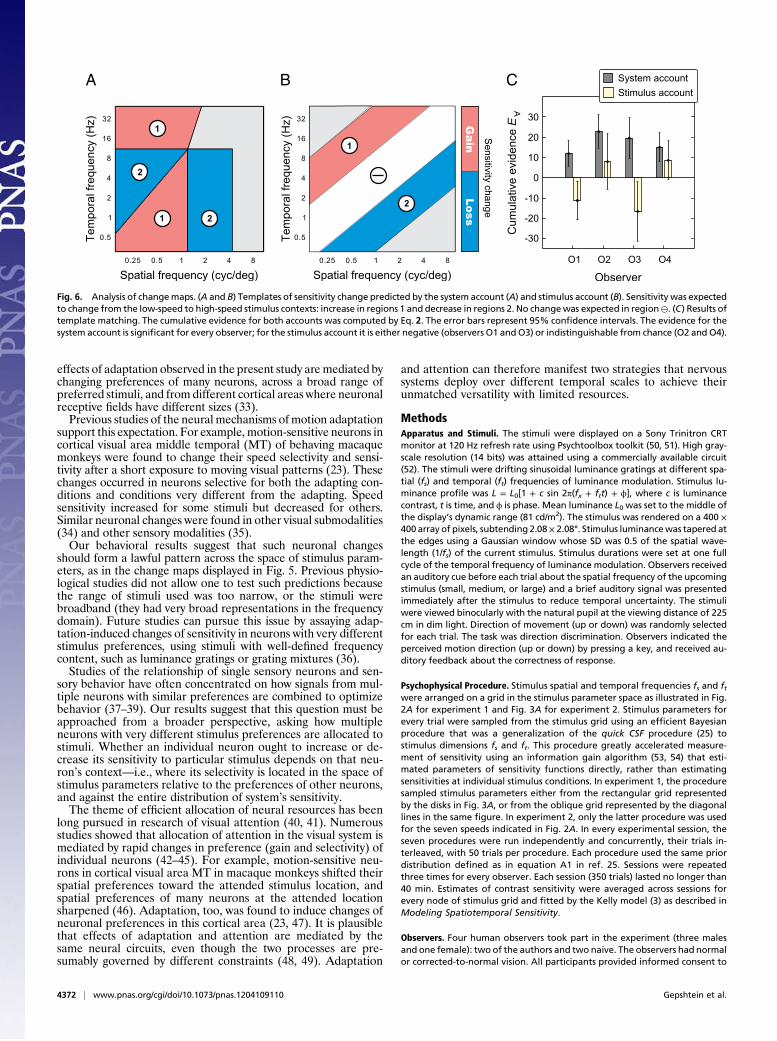
regions where gains and losses of sensitivity were predicted bythe system account, as illustrated in Fig. 6A: gains in regions 1and losses in regions 2. The regions were defined with respect tothe individual maximal-sensitivity sets as explained in SI Methods.In Fig. 5, the regions are demarcated by black lines.To compare our results with predictions of the two accounts in

similar terms, we have also used a stimulus template of sensitivitychange. The stimulus template (Fig. 6B) consisted of regionsbound to the pattern of stimulus change (Fig. 2A). As shown inFig. 6B, gains and losses of sensitivity were expected in regionslabeled 1 and 2, respectively, and no change of sensitivity wasexpected in the region labeled ⊖.The match between the templates of sensitivity change and the

measured changes of sensitivity was quantified using cumulativeevidence

E∀ =Eð+Þ −Eð−Þ; [2]

where E(+) and E(−) were the mean changes of sensitivity re-spectively consistent and inconsistent with the templates (SIMethods). The higher the magnitude of E∀, the better the matchof the data and the template, because the evidence of changesconsistent with the template was positive, and the evidence ofchanges inconsistent with the template was negative.The stimulus template was the same for all observers because

it was defined relative to stimulation, and stimulation did notvary across observers. High evidence E∀ for the stimulus accountwould result if the measured changes of sensitivity followed thesimple pattern captured by the stimulus template.The system template had a different manifestation for every

observer, because the template was defined relative to observer’sindividual sensitivity characteristics. High evidence E∀ for the sys-tem account would result if the measured changes of sensitivityformed a pattern similar to the pattern predicted by the stimulusaccount, i.e., if the gains and losses of sensitivity were arrangedrelative to the maximal-sensitivity sets similar to how they werearranged in the system template.Results of the template-matching analysis are summarized in Fig.

6C. Cumulative evidence E∀ for the system account is representedby the dark bars. In every case, the cumulative evidence was

ytiv iti s

neS

Spatial frequency (cyc/deg)

)zH(

ycneuq erflaropmeT

Spatial frequency (cyc/deg)

BA

)zH(

ycneuqe rf laropm eT

Fig. 3. Results of experiment 1. (A) The circles and lines represent the sam-pled stimulus conditions. We measured “slices” of the spatiotemporal sensi-tivity function: at one spatial or one temporal frequency (one column or onerow of circles), or at one speed (an oblique line). (B) Results of experiment 1 inone observer (O3). The contour plot is an estimate of contrast sensitivityfunction obtained by fitting a standard model (3) to the estimates of sensi-tivity at conditions marked by circles in A. The white crosses mark conditionswhere sensitivity was maximal within the speeds marked by oblique lines in A.

4370 | www.pnas.org/cgi/doi/10.1073/pnas.1204109110 Gepshtein et al.

significantly greater than expected by chance (P < 0.01 for everyobserver, estimated by resampling; SI Methods). The cumulativeevidenceE∀ for the stimulus account is represented by the light bars.Cumulative evidence was against the stimulus account for twoobservers (O1 and O3): the negative values of E∀ were significantlymore negative than expected by chance (P< 0.05 for both observers).

For the two other observers, E∀ was weakly in favor of the stimulusaccount, but it was statistically indistinguishable from chance.

DiscussionWe found that changes in statistics of speed of visual stimuli causeda large-scale reorganization of spatiotemporal contrast sensitivity.Monotonic changes in stimulus speed induced changes of sensi-tivity that were highly nonmonotonic across speed, forming distinctregions of gains and losses of sensitivity summarized by the changemaps in Fig. 5.The results were unlikely to arise from changes in attentional or

decision strategies by our observers. Had the observers registeredthe changes in stimulation and dedicated more attention to themore likely stimuli (26), or had they altered their decision biases inaccord with stimulation (27, 28), changes of performance wouldform a pattern portrayed in Fig. 2B. In the high-speed context thesensitivity would increase for high speeds and decrease for lowspeeds (Fig. 2B), in comparison with the sensitivity in the low-speedcontext. Instead, the changes of sensitivity formed clusters of gainsand losses inconsistent with this stimulus account of adaptation.The observed changes of sensitivity were consistent with the

system account of adaptation (Fig. 2C) in which gains and lossesof sensitivity were expected within high speeds and within lowspeeds. The system account rests on a theory concerned with al-location of limited neural resources in the visual system (24).According to the theory, the spatiotemporal contrast sensitivityfunction (Fig. 1) reflects an optimal allocation of neurons char-acterized by receptive fields of different sizes. The allocationoptimizes sensory performance with respect to the entire ensembleof potential stimuli. Changes in stimulation are therefore expectedto cause changes in characteristics of neurons sensitive to a widerange of stimuli, manifested in a large-scale transformation of thesensitivity function.For two reasons, the present results are likely to generalize to

other stimuli and tasks. First, the differences in visual perfor-mance across stimuli revealed by the spatiotemporally contrastsensitivity function were found to generalize to many stimuli andtasks (29, 30). Second, predictions of the theory of optimal re-source allocation (24) are not confined to contrast sensitivity asa measure of visual performance.What mechanisms are likely to control the efficient allocation of

receptive fields? Studies of cortical neurons selective for movingstimuli have shown that, just as in the somatosensory homunculus(Fig. 1A), the number of neurons selective for a stimulus correlateswith sensitivity to that stimulus. For example, the number ofneurons selective for spatial and temporal frequencies of lumi-nance modulation correlates with the contrast sensitivity at thosespatial frequencies (5, 31, 32) (Fig. 1B). Therefore, it is likely that

A B

Fig. 4. Results of experiment 2. (A) Contrast sensitivityfunctions measured in the two stimulus contexts for oneobserver (O1). A standard model of contrast sensitivitywas fitted to the estimates of sensitivity in high-speed(Upper) and low-speed (Lower) contexts. The warm andcool colors represent high and low sensitivities. Sensi-tivity functions for all observers are displayed in Fig. S2.(B) The change map on the bottom summarizes howsensitivity changed from the low-speed to high-speedstimulus contexts for all stimulus conditions (Eq. 1). Theshades of red and blue represent the gains and losses ofsensitivity, and the white regions represent no change.Above the map, samples of sensitivity changes for twospeeds demonstrate that the pattern of gains and lossesof sensitivity is reversed across speeds, similar to theprediction illustrated in Fig. 2C. Change maps for allobservers are displayed in Fig. 5.

Fig. 5. Change maps. The maps were computed according to Eq. 1. The blacklines demarcate regions where gains and losses of sensitivity were expectedaccording to the system account of adaptation introduced in Fig. 2C. Becauseparameters of individual sensitivity functions varied from across observers,the boundaries between regions of expected gains and losses were derivedindividually, and template structure remained the same (SI Methods). Thenumerical display in the bottom right corner of each panel summarizes howwell the measured change map was matched by the system template (Eq. S1).The larger the index, the better the match. (The change maps are also dis-played in Fig. S2, where changes of sensitivity are scaled by estimation errors,helping to appreciate how effect size varied across stimuli.)

Gepshtein et al. PNAS | March 12, 2013 | vol. 110 | no. 11 | 4371

NEU

ROSC

IENCE

PSYC

HOLO

GICALAND

COGNITIVESC

IENCE

S

effects of adaptation observed in the present study aremediated bychanging preferences of many neurons, across a broad range ofpreferred stimuli, and from different cortical areas where neuronalreceptive fields have different sizes (33).Previous studies of the neural mechanisms of motion adaptation

support this expectation. For example, motion-sensitive neurons incortical visual area middle temporal (MT) of behaving macaquemonkeys were found to change their speed selectivity and sensi-tivity after a short exposure to moving visual patterns (23). Thesechanges occurred in neurons selective for both the adapting con-ditions and conditions very different from the adapting. Speedsensitivity increased for some stimuli but decreased for others.Similar neuronal changes were found in other visual submodalities(34) and other sensory modalities (35).Our behavioral results suggest that such neuronal changes

should form a lawful pattern across the space of stimulus param-eters, as in the change maps displayed in Fig. 5. Previous physio-logical studies did not allow one to test such predictions becausethe range of stimuli used was too narrow, or the stimuli werebroadband (they had very broad representations in the frequencydomain). Future studies can pursue this issue by assaying adap-tation-induced changes of sensitivity in neurons with very differentstimulus preferences, using stimuli with well-defined frequencycontent, such as luminance gratings or grating mixtures (36).Studies of the relationship of single sensory neurons and sen-

sory behavior have often concentrated on how signals from mul-tiple neurons with similar preferences are combined to optimizebehavior (37–39). Our results suggest that this question must beapproached from a broader perspective, asking how multipleneurons with very different stimulus preferences are allocated tostimuli. Whether an individual neuron ought to increase or de-crease its sensitivity to particular stimulus depends on that neu-ron’s context—i.e., where its selectivity is located in the space ofstimulus parameters relative to the preferences of other neurons,and against the entire distribution of system’s sensitivity.The theme of efficient allocation of neural resources has been

long pursued in research of visual attention (40, 41). Numerousstudies showed that allocation of attention in the visual system ismediated by rapid changes in preference (gain and selectivity) ofindividual neurons (42–45). For example, motion-sensitive neu-rons in cortical visual area MT in macaque monkeys shifted theirspatial preferences toward the attended stimulus location, andspatial preferences of many neurons at the attended locationsharpened (46). Adaptation, too, was found to induce changes ofneuronal preferences in this cortical area (23, 47). It is plausiblethat effects of adaptation and attention are mediated by thesame neural circuits, even though the two processes are pre-sumably governed by different constraints (48, 49). Adaptation

and attention can therefore manifest two strategies that nervoussystems deploy over different temporal scales to achieve theirunmatched versatility with limited resources.

MethodsApparatus and Stimuli. The stimuli were displayed on a Sony Trinitron CRTmonitor at 120 Hz refresh rate using Psychtoolbox toolkit (50, 51). High gray-scale resolution (14 bits) was attained using a commercially available circuit(52). The stimuli were drifting sinusoidal luminance gratings at different spa-tial (fs) and temporal (ft) frequencies of luminance modulation. Stimulus lu-minance profile was L = L0[1 + c sin 2π(fx + ftt) + ϕ], where c is luminancecontrast, t is time, and ϕ is phase. Mean luminance L0 was set to the middle ofthe display’s dynamic range (81 cd/m2). The stimulus was rendered on a 400 ×400 array of pixels, subtending 2.08× 2.08°. Stimulus luminancewas tapered atthe edges using a Gaussian window whose SD was 0.5 of the spatial wave-length (1/fs) of the current stimulus. Stimulus durations were set at one fullcycle of the temporal frequency of luminance modulation. Observers receivedan auditory cue before each trial about the spatial frequency of the upcomingstimulus (small, medium, or large) and a brief auditory signal was presentedimmediately after the stimulus to reduce temporal uncertainty. The stimuliwere viewed binocularly with the natural pupil at the viewing distance of 225cm in dim light. Direction of movement (up or down) was randomly selectedfor each trial. The task was direction discrimination. Observers indicated theperceived motion direction (up or down) by pressing a key, and received au-ditory feedback about the correctness of response.

Psychophysical Procedure. Stimulus spatial and temporal frequencies fs and ftwere arranged on a grid in the stimulus parameter space as illustrated in Fig.2A for experiment 1 and Fig. 3A for experiment 2. Stimulus parameters forevery trial were sampled from the stimulus grid using an efficient Bayesianprocedure that was a generalization of the quick CSF procedure (25) tostimulus dimensions fs and ft. This procedure greatly accelerated measure-ment of sensitivity using an information gain algorithm (53, 54) that esti-mated parameters of sensitivity functions directly, rather than estimatingsensitivities at individual stimulus conditions. In experiment 1, the proceduresampled stimulus parameters either from the rectangular grid representedby the disks in Fig. 3A, or from the oblique grid represented by the diagonallines in the same figure. In experiment 2, only the latter procedure was usedfor the seven speeds indicated in Fig. 2A. In every experimental session, theseven procedures were run independently and concurrently, their trials in-terleaved, with 50 trials per procedure. Each procedure used the same priordistribution defined as in equation A1 in ref. 25. Sessions were repeatedthree times for every observer. Each session (350 trials) lasted no longer than40 min. Estimates of contrast sensitivity were averaged across sessions forevery node of stimulus grid and fitted by the Kelly model (3) as described inModeling Spatiotemporal Sensitivity.

Observers. Four human observers took part in the experiment (three malesand one female): two of the authors and two naive. The observers had normalor corrected-to-normal vision. All participants provided informed consent to

A B C

Fig. 6. Analysis of changemaps. (A and B) Templates of sensitivity change predicted by the system account (A) and stimulus account (B). Sensitivity was expectedto change from the low-speed to high-speed stimulus contexts: increase in regions 1 and decrease in regions 2. No changewas expected in region⊖. (C) Results oftemplate matching. The cumulative evidence for both accounts was computed by Eq. 2. The error bars represent 95% confidence intervals. The evidence for thesystem account is significant for every observer; for the stimulus account it is either negative (observers O1 andO3) or indistinguishable from chance (O2 and O4).

4372 | www.pnas.org/cgi/doi/10.1073/pnas.1204109110 Gepshtein et al.

participate in the experiment. The experiments followed a protocol ap-proved by the Salk Institute’s Institutional Research Board.

Modeling Spatiotemporal Sensitivity. Analysis of contrast sensitivity wasperformed both using the raw estimates of sensitivity produced by ourpsychophysical procedure for nodes of the stimulus grid, and using fittedfunctions of spatiotemporal contrast sensitivity. The fits were derivedusing the Kelly function (i.e., equation 5 in ref. 3): G(α, υ) = kυα2exp(−2α/αmax), where υ is speed, α is a constant inferred by Kelly from spatialfrequency characteristics of receptive fields, and k and αmax are speed-dependent coefficients. The raw estimates were obtained for 36 stimulusconditions in experiment 1 (Fig. 2A) and for 56 conditions in experiment2 (Fig. 2A).

Kelly function was fitted to the raw estimates of sensitivity on a grid of 60spatial and 80 temporal frequency conditions, the same in experiments 1 and 2.The fits accounted for the average of 84% of the variability (R2) of raw sen-sitivity estimates (SD 8%). Using permutation analysis, we found that theprobability to obtain such a fit by chance was smaller than 0.01, for allobservers. (The individual coefficients of determination R2 were 0.81, 0.91,0.75, and 0.92 for observers O1–O4, respectively.) Maximal-sensitivity setsand were estimated for the high-speed and low-speed stimulus contexts,

respectively, by finding the stimulus conditions at which the Kelly models hadmaximal values on multiple constant-speed lines. Parameters of andwere used to derive the templates of sensitivity change described below.

Permutation Analysis of Sensitivity. We evaluated differences between con-trast sensitivity estimates from different stimulus contexts using standardrandomization methods. Sensitivity estimates in each stimulus context wererandomly and repeatedly permuted, and root mean square differences Dk

between the permuted estimates were computed on each iteration K,forming distribution D of such differences. Fraction p of D that was smallerthan zero was an estimate of the probability that the measured differencebetween sensitivities in the two stimulus contexts occurred by chance.

ACKNOWLEDGMENTS. We thank C. F. Stevens and I. Tyukin for discussions;P. Jurica for assistance in developing the software for data analysis;J. H. Reynolds and G. Stoner for comments on the manuscript; and the lateM. Mitchell for administrative assistance. This work was supported by theSwartz Foundation; National Science Foundation Grant 1027259 (to S.G.);the Kavli Foundation; National Institutes of Health Grants EY018613 (to S.G.and T.D.A.) and EY01711 and EY018664 (L.A.L.); and National Eye InstituteCore Grant for Vision Research P-30-EY019005.

1. Penfield W, Erickson TC (1941) Epilepsy and Cerebral Localization: A Study of theMechanism, Treatment and Prevention of Epileptic Seizures (Charles C. Thomas,Springfield, IL).

2. Weinstein S (1968) The Skin Senses, ed Kenshalo DR (Charles C. Thomas, Springfield,IL), pp 195–222.

3. Kelly DH (1979) Motion and vision. II. Stabilized spatio-temporal threshold surface. JOpt Soc Am 69(10):1340–1349.

4. De Valois RL, Albrecht DG, Thorell LG (1982) Spatial frequency selectivity of cells inmacaque visual cortex. Vision Res 22(5):545–559.

5. De Valois RL, De Valois KK (1990) Spatial Vision (Oxford Univ Press, New York).Available at http://www.sciencedirect.com/science/journal/00426989.

6. Banks MS, Geisler WS, Bennett PJ (1987) The physical limits of grating visibility. VisionRes 27(11):1915–1924.

7. Van Hateren JH (1993) Spatiotemporal contrast sensitivity of early vision. Vision Res33(2):257–267.

8. Geisler WS, Albrecht DG (2000) Handbook of Perception and Cognition. Seeing, ed DeValois KK (Academic, San Diego), 2nd Ed, pp 79–128.

9. Bex PJ, Makous W (2002) Spatial frequency, phase, and the contrast of natural im-ages. J Opt Soc Am A Opt Image Sci Vis 19(6):1096–1106.

10. Barlow HB (1961) Sensory Communication, ed Rosenbluth WA (MIT Press, Cambridge,MA), pp 217–234.

11. Wainwright MJ (1999) Visual adaptation as optimal information transmission. VisionRes 39(23):3960–3974.

12. Sharpee TO, et al. (2006) Adaptive filtering enhances information transmission invisual cortex. Nature 439(7079):936–942.

13. Blakemore C, Campbell FW (1969) On the existence of neurones in the human visualsystem selectively sensitive to the orientation and size of retinal images. J Physiol203(1):237–260.

14. Blakemore C, Sutton P (1969) Size adaptation: A new aftereffect. Science 166(3902):245–247.

15. Davis ET, Graham N (1981) Spatial frequency uncertainty effects in the detection ofsinusoidal gratings. Vision Res 21(5):705–712.

16. Barlow HB, Macleod DIA, van Meeteren A (1976) Adaptation to gratings: No com-pensatory advantages found. Vision Res 16(10):1043–1045.

17. Movshon JA, Lennie P (1979) Pattern-selective adaptation in visual cortical neurones.Nature 278(5707):850–852.

18. Hübner R (1996) Specific effects of spatial-frequency uncertainty and different cuetypes on contrast detection: Data and models. Vision Res 36(21):3429–3439.

19. Zhang P, Bao M, Kwon M, He S, Engel SA (2009) Effects of orientation-specific visualdeprivation induced with altered reality. Curr Biol 19(22):1956–1960.

20. De Valois KK (1977) Spatial frequency adaptation can enhance contrast sensitivity.Vision Res 17(9):1057–1065.

21. Regan D, Beverley KI (1985) Postadaptation orientation discrimination. J Opt Soc AmA 2(2):147–155.

22. Clifford CWG, Wenderoth P (1999) Adaptation to temporal modulation can enhancedifferential speed sensitivity. Vision Res 39(26):4324–4332.

23. Krekelberg B, van Wezel RJ, Albright TD (2006) Adaptation in macaque MT reducesperceived speed and improves speed discrimination. J Neurophysiol 95(1):255–270.

24. Gepshtein S, Tyukin I, Kubovy M (2007) The economics of motion perception andinvariants of visual sensitivity. J Vis 7(8):8.1–18.

25. Lesmes LA, Lu ZL, Baek J, Albright TD (2010) Bayesian adaptive estimation of thecontrast sensitivity function: The quick CSF method. J Vis 10(3):17.1–21.

26. Epstein W, Rock I (1960) Perceptual set as an artifact of recency. Am J Psychol 73(2):214–228.

27. Burgess A (1985) Visual signal detection. III. On Bayesian use of prior knowledge andcross correlation. J Opt Soc Am A 2(9):1498–1507.

28. Maloney LT, Zhang H (2010) Decision-theoretic models of visual perception and ac-

tion. Vision Res 50(23):2362–2374.29. Watson AB, Barlow HB, Robson JG (1983) What does the eye see best? Nature 302

(5907):419–422.30. Nakayama K (1985) Biological image motion processing: A review. Vision Res 25(5):

625–660.31. Movshon JA, Thompson ID, Tolhurst DJ (1978) Spatial and temporal contrast sensi-

tivity of neurones in areas 17 and 18 of the cat’s visual cortex. J Physiol 283:101–120.32. Thiele A, Dobkins KR, Albright TD (1999) The contribution of color to motion pro-

cessing in Macaque middle temporal area. J Neurosci 19(15):6571–6587.33. Priebe NJ, Lisberger SG, Movshon JA (2006) Tuning for spatiotemporal frequency and

speed in directionally selective neurons of macaque striate cortex. J Neurosci 26(11):

2941–2950.34. Crowder NA, et al. (2006) Relationship between contrast adaptation and orientation

tuning in V1 and V2 of cat visual cortex. J Neurophysiol 95(1):271–283.35. Dean I, Harper NS, McAlpine D (2005) Neural population coding of sound level adapts

to stimulus statistics. Nat Neurosci 8(12):1684–1689.36. Priebe NJ, Cassanello CR, Lisberger SG (2003) The neural representation of speed in

macaque area MT/V5. J Neurosci 23(13):5650–5661.37. Geisler WS, Albrecht DG (1997) Visual cortex neurons in monkeys and cats: Detection,

discrimination, and identification. Vis Neurosci 14(5):897–919.38. Parker AJ, Newsome WT (1998) Sense and the single neuron: Probing the physiology

of perception. Annu Rev Neurosci 21:227–277.39. Ma WJ, Beck JM, Latham PE, Pouget A (2006) Bayesian inference with probabilistic

population codes. Nat Neurosci 9(11):1432–1438.40. Sperling G, Dosher BA (1986) Handbook of Perception and Performance, eds Boff K,

et al. (Wiley, New York), Vol 1, pp 2.1–2.65.41. Desimone R, Duncan J (1995) Neural mechanisms of selective visual attention. Annu

Rev Neurosci 18:193–222.42. Moran J, Desimone R (1985) Selective attention gates visual processing in the ex-

trastriate cortex. Science 229(4715):782–784.43. Reynolds JH, Pasternak T, Desimone R (2000) Attention increases sensitivity of V4

neurons. Neuron 26(3):703–714.44. David SV, Hayden BY, Mazer JA, Gallant JL (2008) Attention to stimulus features shifts

spectral tuning of V4 neurons during natural vision. Neuron 59(3):509–521.45. Bisley JW (2011) The neural basis of visual attention. J Physiol 589(Pt 1):49–57.46. Womelsdorf T, Anton-Erxleben K, Treue S (2008) Receptive field shift and shrinkage in

macaque middle temporal area through attentional gain modulation. J Neurosci

28(36):8934–8944.47. Kohn A, Movshon JA (2004) Adaptation changes the direction tuning of macaque MT

neurons. Nat Neurosci 7(7):764–772.48. Pestilli F, Viera G, Carrasco M (2007) How do attention and adaptation affect contrast

sensitivity? J Vis 7(7):9.1–12.49. Webster MA (2011) Adaptation and visual coding. J Vis 11(5):3.1–23.50. Brainard DH (1997) The psychophysics toolbox. Spat Vis 10(4):433–436.51. Pelli DG (1997) The VideoToolbox software for visual psychophysics: transforming

numbers into movies. Spat Vis 10(4):437–442.52. Li X, Lu ZL, Xu P, Jin J, Zhou Y (2003) Generating high gray-level resolution mono-

chrome displays with conventional computer graphics cards and color monitors. J

Neurosci Methods 130(1):9–18.53. Kontsevich LL, Tyler CW (1999) Bayesian adaptive estimation of psychometric slope

and threshold. Vision Res 39(16):2729–2737.54. Kujala J, Lukka T (2006) Bayesian adaptive estimation: The next dimension. J

Math Psychol 50(4):369–389.

Gepshtein et al. PNAS | March 12, 2013 | vol. 110 | no. 11 | 4373

NEU

ROSC

IENCE

PSYC

HOLO

GICALAND

COGNITIVESC

IENCE

S