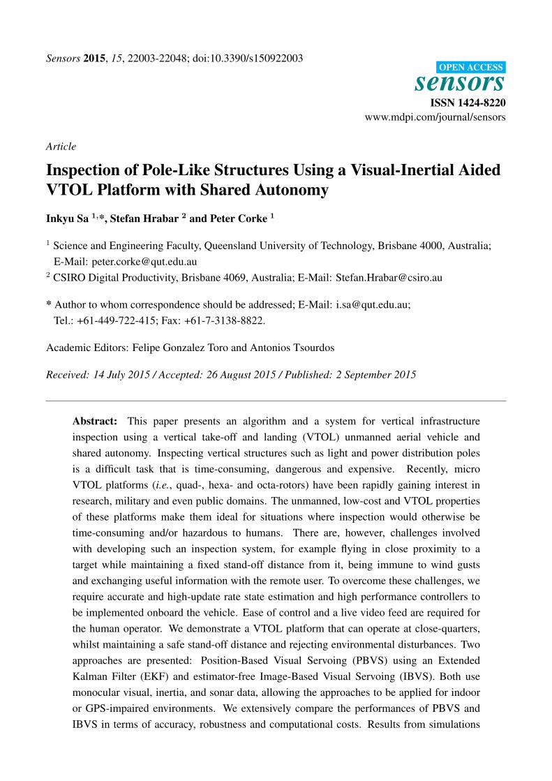
Sensors 2015, 15, 22003-22048; doi:10.3390/s150922003OPEN ACCESS

sensorsISSN 1424-8220

www.mdpi.com/journal/sensors

Article

Inspection of Pole-Like Structures Using a Visual-Inertial AidedVTOL Platform with Shared AutonomyInkyu Sa 1,*, Stefan Hrabar 2 and Peter Corke 1

1 Science and Engineering Faculty, Queensland University of Technology, Brisbane 4000, Australia;E-Mail: peter.corke@qut.edu.au

2 CSIRO Digital Productivity, Brisbane 4069, Australia; E-Mail: Stefan.Hrabar@csiro.au

* Author to whom correspondence should be addressed; E-Mail: i.sa@qut.edu.au;Tel.: +61-449-722-415; Fax: +61-7-3138-8822.

Academic Editors: Felipe Gonzalez Toro and Antonios Tsourdos

Received: 14 July 2015 / Accepted: 26 August 2015 / Published: 2 September 2015

Abstract: This paper presents an algorithm and a system for vertical infrastructureinspection using a vertical take-off and landing (VTOL) unmanned aerial vehicle andshared autonomy. Inspecting vertical structures such as light and power distribution polesis a difficult task that is time-consuming, dangerous and expensive. Recently, microVTOL platforms (i.e., quad-, hexa- and octa-rotors) have been rapidly gaining interest inresearch, military and even public domains. The unmanned, low-cost and VTOL propertiesof these platforms make them ideal for situations where inspection would otherwise betime-consuming and/or hazardous to humans. There are, however, challenges involvedwith developing such an inspection system, for example flying in close proximity to atarget while maintaining a fixed stand-off distance from it, being immune to wind gustsand exchanging useful information with the remote user. To overcome these challenges, werequire accurate and high-update rate state estimation and high performance controllers tobe implemented onboard the vehicle. Ease of control and a live video feed are required forthe human operator. We demonstrate a VTOL platform that can operate at close-quarters,whilst maintaining a safe stand-off distance and rejecting environmental disturbances. Twoapproaches are presented: Position-Based Visual Servoing (PBVS) using an ExtendedKalman Filter (EKF) and estimator-free Image-Based Visual Servoing (IBVS). Both usemonocular visual, inertia, and sonar data, allowing the approaches to be applied for indooror GPS-impaired environments. We extensively compare the performances of PBVS andIBVS in terms of accuracy, robustness and computational costs. Results from simulations

Sensors 2015, 15 22004

and indoor/outdoor (day and night) flight experiments demonstrate the system is able tosuccessfully inspect and circumnavigate a vertical pole.

Keywords: aerial robotics; pole inspection; visual servoing, shared autonomy

1. Introduction

This paper presents an inspection system based on a vertical take-off landing (VTOL) platformand shared autonomy. The term “shared autonomy” indicates that the major fraction of control isaccomplished by a computer. The operator’s interventions for low-level control are prohibited butthe operator provides supervisory high-level control commands such as setting the goal position. Inorder to perform an inspection task, a VTOL platform should fly in close proximity to the target objectbeing inspected. This close-quarters flying does not require global navigation (explorations of largeknown or unknown environments) but instead requires local navigation relative to the specific geometryof the target, for instance, the pole of a streetlight. Such a system allows an unskilled operator toeasily and safely control a VTOL platform to examine locations that are otherwise difficult to reach.For example, it could be used for practical tasks such as inspecting for bridge or streetlight defects.Inspection is an important task for the safety of structures but is a dangerous and labor intensive job.According to the US Bureau of Transportation Statistics, there are approximately 600,000 bridges in theUnited States and 26% of them require inspections. Echelon, an electricity company, reported that thereare 174.1 million streetlights in the US, Europe, and UK [1]. These streetlights also require inspectionsevery year. These tasks are not only high risk for the workers involved but are slow, labour intensive andtherefore expensive. VTOL platforms can efficiently perform these missions since they can reach placesthat are high and inaccessible such as the outsides of buildings (roof or wall), high ceilings, the tops ofpoles and so on. However, it is very challenging to use these platforms for inspection because there isinsufficient room for error and high-level pilot skills are required as well as line-of-sight from pilot tovehicle. This paper is concerned with enabling low-cost semi-autonomous flying robots, in collaborationwith low-skilled human operators, to perform useful tasks close to objects.

Multi-rotor VTOL micro aerial vehicles (MAVs) have been popular research platforms for a numberof years due to advances in sensor, battery and integrated circuit technologies. The variety ofcommercially-available platforms today is testament to the fact that they are leaving the research labs andbeing used for real-world aerial work. These platforms are very capable in terms of their autonomousor attitude stabilized flight modes and the useful payloads they can carry. Arguably the most commonuse is for the collection of aerial imagery, for applications such as mapping, surveys, conservation andinfrastructure inspection. Applications such as infrastructure inspection require flying at close-quarters tovertical structures in order to obtain the required images. Current regulations require the MAV’s operatorto maintain visual line-of-sight contact with the aircraft, but even so it is an extremely challenging taskfor the operator to maintain a safe, fixed distance from the infrastructure being inspected. From thevantage point on the ground it is hard to judge the stand-off distance, and impossible to do so once theaircraft is obscured by the structure. The problem is exacerbated in windy conditions as the structures

Sensors 2015, 15 22005

cause turbulence. The use of First-Person View (FPV) video streamed live from the platform can helpwith situational awareness, but flying close to structures still requires great skill and experience by theoperator and requires a reliable low-latency high-bandwidth communication channel. It has been foundthat flight operations near vertical structures is best performed by a team of three people: a skilled pilot,a mission specialist, and a flight director [2]. For small VTOL MAVs to truly become ubiquitous aerialimaging tools that can be used by domain experts rather than skilled pilots, their level of autonomy mustbe increased. One avenue to increased autonomy of a platform is through shared autonomy, where themajority of control is accomplished by the platform, but operator input is still required. Typically, theoperator is relieved from the low-level relative-control task which is better performed by a computer, butstill provides supervisory high-level control commands such as a goal position. We employ this sharedautonomy approach for the problem of MAV-based vertical infrastructure inspections.

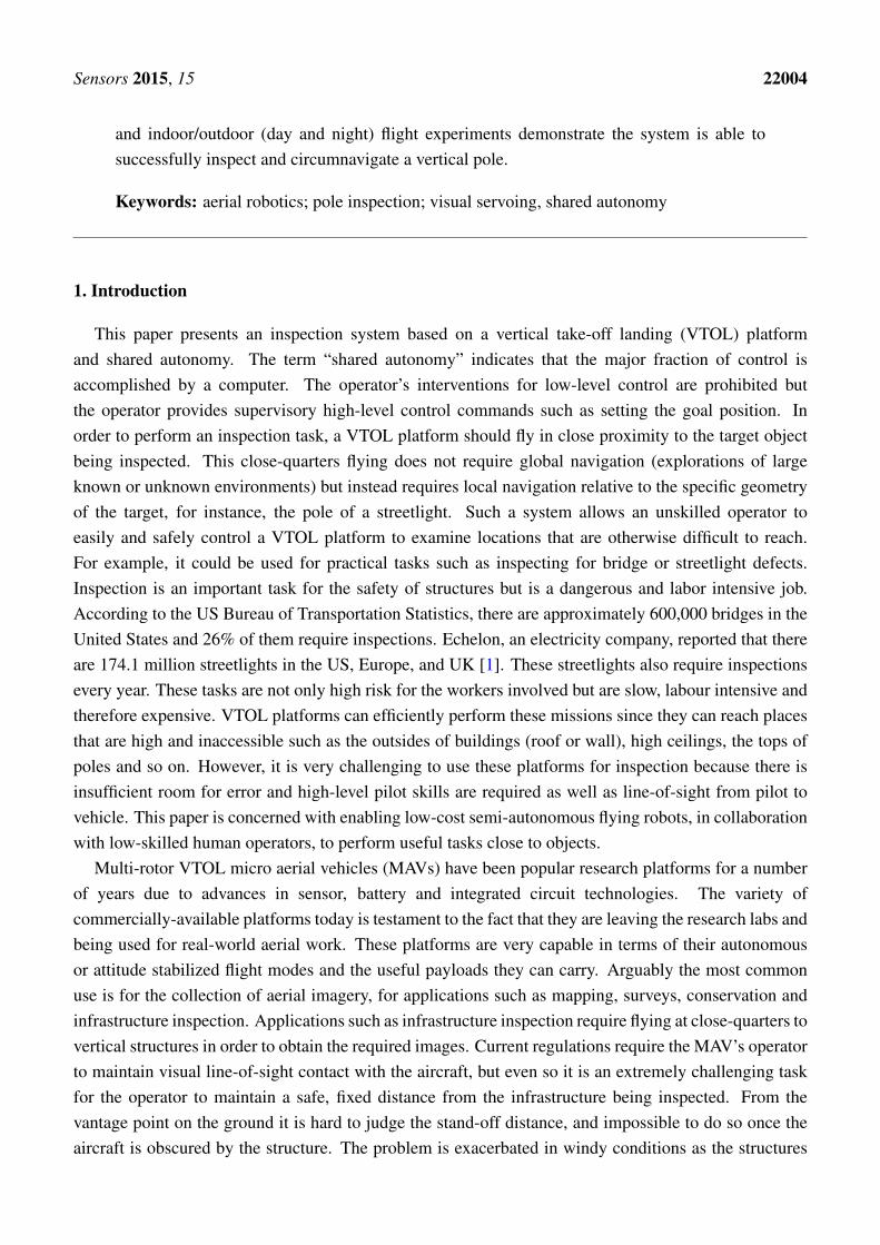
It is useful for an operator to be able to “guide” the MAV in order to obtain the required inspectionviewpoints without the cognitive workload of “piloting” it. We provide the additional autonomy neededby implementing visual plus inertial-based pole-relative hovering as well as object circumnavigationshown in Figure 1. By tracking the two edges of the pole in the image and employing Position-BasedVisual Servoing (PBVS) or Image-Based Visual Servoing (IBVS), the platform is able to maintain a userspecified distance from the pole and keep the camera oriented towards the pole. The operator is also ableto control the height and yaw of the platform. Since the pole is kept centred in the image, a yaw ratecontrol command results in an orbit about the pole. A cylindrical workspace around the pole is thereforeavailable to the operator for manoeuvres.

Figure 1. The vertical take-off and landing (VTOL) platform used for our pole inspectionexperiments. It includes a front-facing camera, downward-facing ultrasonic sensor and anonboard inertial measurement unit (IMU) for attitude control. All processing occurs onboardusing a quad-core Acorn Risc Machine (ARM) Cortex-A9 processor.

1.1. Related Work

1.1.1. Climbing Robots for Inspection Tasks

As mentioned before, inspecting structures, such as light and power distribution poles is atime-consuming, dangerous and expensive task with high operator workload. The options for inspectinglocations above the ground are rather limited, and all are currently cumbersome. Ladders can be used up

Sensors 2015, 15 22006

to a height of 10–15 m but are quite dangerous: each year 160 people are killed and 170,000 injured infalls from ladders in the United States [3]. Cherry pickers require large vehicle access, sufficient spaceto operate and considerable setup time.

Robotics and mechatronics researchers have demonstrated a variety of climbing robots. Considerablegrowth in sensor and integrated circuit technology has accelerated small and lightweight roboticsdevelopment. Typically, these robots are inspired by reptiles, mammals and insects, and their type ofmovement varies between sliding, swinging, extension and jumping.

The flexible mechatronic assistive technology system (MATS) robot has five degrees of freedom(DOF) and a symmetrical mechanism [4]. The robot shows good mobility features for travel, however,it requires docking stations that are attached to the wall, ceiling, or anywhere the robot is required totraverse. The bio-mimicking gekko robot, StickyBot [5], does not require docking stations since it hashierarchical adhesive structures under its toes to hold itself on any kind of surface. It has, however,limitations for payload and practical applications. A bridge cable inspection robot [6] is more applicablethan the StickyBot in terms of its climbing speed and payload carrying ability. It climbs the cables bymeans of wheels which remain in contact with the cable for traction. A climbing robot with leggedlocomotion was developed by Haynes et al. [7]. This robot was designed for high-speed climbing of auniformly convex cylindrical structure, such as a telephone or electricity pole. NASA’s Jet PropulsionLaboratory recently demonstrated a rock climbing robot utilizing a hierarchical array of claws (calledmicrospines) to create an attachment force of up to 180 N normal to the surface [8]. This robot also candrill a hole with a self-contained rotary percussive drill while it is attached to the surface.

Since climbing robots are in contact with the surface they can perform contact-based high-precisioninspection with high performance sensors. They are also able to perform physical actions on the surface,not just inspections [9]. These climbing robots could not only replace a worker undertaking risky tasks ina hazardous environment but also increase the efficiency of such tasks. Climbing robots, however, requirecomplex mechanical designs and complicated dynamic analysis. Their applications are also limited tostructures with specific shapes and surface materials. They require setup time and climb slowly, so theinspection task can be time-consuming.

1.1.2. Flying Robots for Inspection Tasks

VTOL platforms on the other hand offer a number of advantages when used for infrastructureinspection. They have relatively simple mechanical designs (usually symmetric) which require a simpledynamic analysis and controller. VTOL platforms can ascend quickly to the required height and canobtain images from many angles regardless of the shape of the structure. Recent advanced sensor,integrated circuit and motor technologies allow VTOL platforms to fly for a useful amount of time whilecarrying inspection payloads. Minimal space is required for operations and their costs are relatively low.The popularity of these platforms means that hardware and software resources are readily available [10].

These advantages have accelerated the development of small and light-weight flying robotics forinspection. Voigt et al. [11] demonstrated an embedded stereo-camera based egomotion estimationtechnique for the inspection of structures such as boilers and general indoor scenarios. The stereo visionsystem provides a relative pose estimate between the previous and the current frame and this is fed into anindirect Extended Kalman Filter (EKF) framework as a measurement update. The inertial measurements

Sensors 2015, 15 22007

such as linear accelerations and rotation rates played important roles in the filter framework. States,(position, orientation, bias, and relative pose) were propagated with IMU measurements through aprediction step and the covariance of the predicted pose were exploited to determine a confidence regionfor feature searching in the image plane. This allowed feature tracking on scenes with repeating textures(perception aliasing), increased the total number of correct matches (inliers), and efficiently rejectedoutliers with reasonable computation power. They evaluated the proposed method on several trajectorieswith varying flight velocities. The results presented show the vehicle is capable of impressively accuratepath tracking. However, flights tests were performed indoors in a boiler mock-up environment wheredisturbances are not abundant, and using hand-held sequences from an office building dataset. Basedon this work, Burri et al. [12] and Nikolic et al. [13] show visual inspection of a thermal powerplant boiler system using a quadrotor. They developed a Field Programmable Gate Array (FPGA)based visual-inertial stereo Simultaneous Localization and Mapping (SLAM) sensor with state updatesat 10 Hz. A model predictive controller (MPC) is used for closed loop control in industrial boilerenvironments. In contrast to their work, we aim for flights in outdoor environments where disturbancessuch as wind gusts are abundant and the scenes include natural objects.

Ortiz et al. [14] and Eich et al. [15] introduced autonomous vessel inspection using a quadrotorplatform. A laser scanner is utilized for horizontal pose estimation with Rao-Blackwellized particlefilter based SLAM (GMapping), and small mirrors reflected a few of the horizontal beams verticallydownwards for altitude measurement. These technologies have been adopted from the 2D ground vehicleSLAM solution into aerial vehicle research [16] and often incorporated within a filter framework for fastupdate rates and accurate state estimation [17]. While such methods are well-established and optimizedopen-source software packages are available, one of the main drawbacks is the laser scanner. Comparedto monocular vision, a laser scanner is relatively heavy and consumes more power, which significantlydecreases the total flight time. Instead, we propose a method using only a single light-weight camera, ageometric model of the target object, and a single board computer for vertical structure inspection tasks.

1.2. Contributions and Overview

This paper contributes to the state-of-the-art in aerial inspections by addressing the limitations ofexisting approaches presented in Section 1.1 with the proposed high performance vertical structureinspection system. In this paper, we make use of our previous developed robust line feature tracker [18]as a front-end vision system, and it is summarized in Section 2.2. A significant difference to our previousworks [19–21] in which different flying platforms had been utilized is the integration of both PBVS andIBVS systems on the same platform. By doing so, we are able to compare both systems quantitatively.We also conduct experiments where a trained pilot performs the same tasks using manual flight andwith the aid of PBVS and IBVS and demonstrate the difficulty of the tasks. For evaluation, motioncapture systems, a laser tracker, and hand-annotated images are used. Therefore, the contributions ofthis paper are:

• The development of onboard flight controllers using monocular visual features (lines) and inertialsensing for visual servoing (PBVS and IBVS) to enable VTOL MAV close quarters manoeuvring.

Sensors 2015, 15 22008

• The use of shared autonomy to permit an un-skilled operator to easily and safely performMAV-based pole inspections in outdoor environments, with wind, and at night.

• Significant experimental evaluation of state estimation and control performance for indoor andoutdoor (day and night) flight tests, using a motion capture device and a laser tracker for groundtruth. Video demonstration [22].

• A performance evaluation of the proposed systems in comparison to skilled pilots for a poleinspection task.

The remainder of the paper is structured as follows: Section 2 describes the coordinate systemdefinition used in this paper, and the vision processing algorithms for fast line tracking. Sections 3 and 4present the PBVS and IBVS control structures which are developed for the pole inspection scenario, andwith validation through simulation. Section 5 presents the use of shared autonomy and we present ourextensive experimental results in Section 6. Conclusions are drawn in Section 7.

2. Coordinate Systems and Image Processing

2.1. Coordinate Systems

We define three right-handed frames: world {W}, body {B} and camera {C} which are shown inFigure 2. Note that both {W} and {B} have their z-axis downward while {C} has its z-axis (cameraoptical axis) in the horizontal plane of the propellers and pointing in the vehicle’s forward direction. Wedefine the notation aRb which rotates a vector defined with respect to frame {b} to a vector with respectto {a}.

y

x

z

{W}y

x

z{B}

yx z{C}

WRB, t0

BRC , t1

Camera

{W} = World frame

{B} = Body frame

{C} = Camera frame

tn = Translation

Rn = Rotation

Figure 2. Coordinate systems: body {B}, world {W}, and camera {C}. Transformationbetween {B} and {C} is constant whereas {B} varies as the quadrotor moves. CRB rotates avector defined with respect to {B} to a vector with respect to {C}.

2.2. Image Processing for Fast Line Tracking

Our line tracker is based on tracking the two edges of the pole over time. This is an appropriatefeature since the pole will dominate the scene in our selected application. There are many reported lineextraction algorithms such as Hough transform [23] and other linear feature extractors [24] but thesemethods are unsuitable due to their computational complexity. Instead we use a simple and efficient linetracker inspired by [25]. The key advantage of this algorithm is its low computation requirement. For320× 240 pixel images every iteration is finished in < 16 ms and uses only 55% of the CPU quad-coreARM Cortex-A9.

Sensors 2015, 15 22009

2.2.1. 2D and 3D Line Models

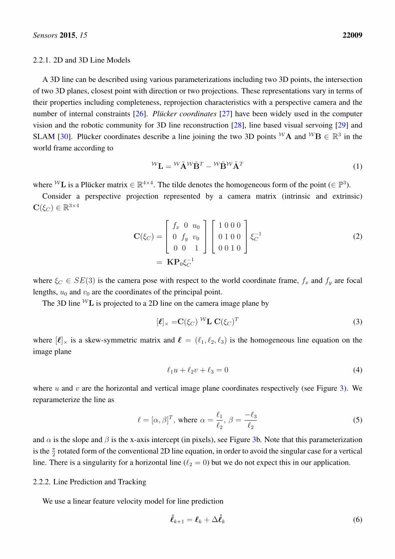
A 3D line can be described using various parameterizations including two 3D points, the intersectionof two 3D planes, closest point with direction or two projections. These representations vary in terms oftheir properties including completeness, reprojection characteristics with a perspective camera and thenumber of internal constraints [26]. Plücker coordinates [27] have been widely used in the computervision and the robotic community for 3D line reconstruction [28], line based visual servoing [29] andSLAM [30]. Plücker coordinates describe a line joining the two 3D points WA and WB ∈ R3 in theworld frame according to

WL = WAWBT − WBWAT (1)

where WL is a Plücker matrix ∈ R4×4. The tilde denotes the homogeneous form of the point (∈ P3).Consider a perspective projection represented by a camera matrix (intrinsic and extrinsic)

C(ξC) ∈ R3×4

C(ξC) =

fx 0 u0

0 fy v0

0 0 1

1 0 0 0

0 1 0 0

0 0 1 0

ξ−1C (2)

= KP0ξ−1C

where ξC ∈ SE(3) is the camera pose with respect to the world coordinate frame, fx and fy are focallengths, u0 and v0 are the coordinates of the principal point.

The 3D line WL is projected to a 2D line on the camera image plane by

[`]× =C(ξC) WL C(ξC)T (3)

where [`]× is a skew-symmetric matrix and ` = (`1, `2, `3) is the homogeneous line equation on theimage plane

`1u+ `2v + `3 = 0 (4)

where u and v are the horizontal and vertical image plane coordinates respectively (see Figure 3). Wereparameterize the line as

` = [α, β]T , where α =`1`2, β =

−`3`2

(5)

and α is the slope and β is the x-axis intercept (in pixels), see Figure 3b. Note that this parameterizationis the π

2rotated form of the conventional 2D line equation, in order to avoid the singular case for a vertical

line. There is a singularity for a horizontal line (`2 = 0) but we do not expect this in our application.

2.2.2. Line Prediction and Tracking

We use a linear feature velocity model for line prediction

ˆk+1 = `k + ∆ ˙

k (6)

Sensors 2015, 15 22010

where k is the timestep, ˆk+1 is the predicted line in the image plane, ˙k is the feature velocity, `k is the

previously observed feature and ∆ is the sample time. In order to calculate feature velocity, we computean image Jacobian, Jl, which describes how a line moves on the image plane as a function of cameraspatial velocity ν = [C x, C y, C z, Cωx,

Cωy,Cωz]

T [31].

˙k = Jlkνk (7)

This image Jacobian is the derivative of the 3D line projection function with respect to camera pose,and for the line parameterization of Equation (5) Jl ∈ R2×6.

yx

z

a

!

b

image plane

WA

WB

WL

{C}

(a)

!"#$%&'()*+,-./0123456789:;<=>?@ABCDEFGHIJKLMNOPQRSTUVWXYZ[\]_abcdefghijklmnopqrstuvwxyz{|}~

u

v

(u0, v0)

!

(W, H)

α >0α <0

β

α=0

(b)

Figure 3. (a) Perspective image of a line WL in 3D space. a and b are projections of theworld point and ` is a line on the image plane; (b) Image plane representation of slope (α)and intercept (β).

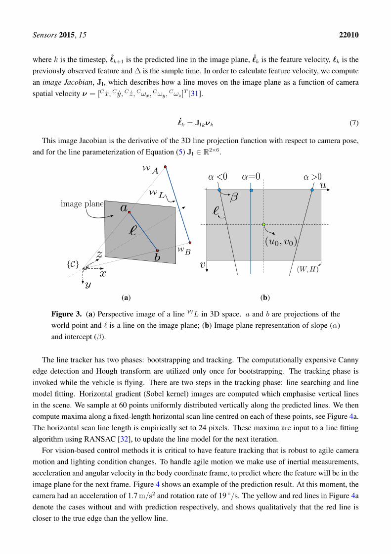
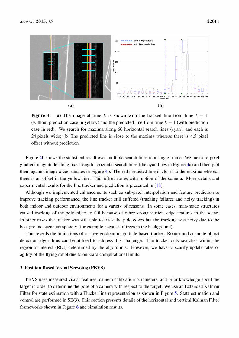
The line tracker has two phases: bootstrapping and tracking. The computationally expensive Cannyedge detection and Hough transform are utilized only once for bootstrapping. The tracking phase isinvoked while the vehicle is flying. There are two steps in the tracking phase: line searching and linemodel fitting. Horizontal gradient (Sobel kernel) images are computed which emphasise vertical linesin the scene. We sample at 60 points uniformly distributed vertically along the predicted lines. We thencompute maxima along a fixed-length horizontal scan line centred on each of these points, see Figure 4a.The horizontal scan line length is empirically set to 24 pixels. These maxima are input to a line fittingalgorithm using RANSAC [32], to update the line model for the next iteration.

For vision-based control methods it is critical to have feature tracking that is robust to agile cameramotion and lighting condition changes. To handle agile motion we make use of inertial measurements,acceleration and angular velocity in the body coordinate frame, to predict where the feature will be in theimage plane for the next frame. Figure 4 shows an example of the prediction result. At this moment, thecamera had an acceleration of 1.7 m/s2 and rotation rate of 19 ◦/s. The yellow and red lines in Figure 4adenote the cases without and with prediction respectively, and shows qualitatively that the red line iscloser to the true edge than the yellow line.

Sensors 2015, 15 22011

(a)

0

50

100

150

200

250

79 80 81 82 83 84 85 86 87 88 89 90 91 92 93 94 95 96 97 98 99 100 101 102U coordinate

Pixe

l int

ensi

ty

with line predictionw/o line predictionw/o line prediction

with line prediction

(b)

Figure 4. (a) The image at time k is shown with the tracked line from time k − 1

(without prediction case in yellow) and the predicted line from time k − 1 (with predictioncase in red). We search for maxima along 60 horizontal search lines (cyan), and each is24 pixels wide; (b) The predicted line is close to the maxima whereas there is 4.5 pixeloffset without prediction.

Figure 4b shows the statistical result over multiple search lines in a single frame. We measure pixelgradient magnitude along fixed length horizontal search lines (the cyan lines in Figure 4a) and then plotthem against image u coordinates in Figure 4b. The red predicted line is closer to the maxima whereasthere is an offset in the yellow line. This offset varies with motion of the camera. More details andexperimental results for the line tracker and prediction is presented in [18].

Although we implemented enhancements such as sub-pixel interpolation and feature prediction toimprove tracking performance, the line tracker still suffered (tracking failures and noisy tracking) inboth indoor and outdoor environments for a variety of reasons. In some cases, man-made structurescaused tracking of the pole edges to fail because of other strong vertical edge features in the scene.In other cases the tracker was still able to track the pole edges but the tracking was noisy due to thebackground scene complexity (for example because of trees in the background).

This reveals the limitations of a naive gradient magnitude-based tracker. Robust and accurate objectdetection algorithms can be utilized to address this challenge. The tracker only searches within theregion-of-interest (ROI) determined by the algorithms. However, we have to scarify update rates oragility of the flying robot due to onboard computational limits.

3. Position Based Visual Servoing (PBVS)

PBVS uses measured visual features, camera calibration parameters, and prior knowledge about thetarget in order to determine the pose of a camera with respect to the target. We use an Extended KalmanFilter for state estimation with a Plücker line representation as shown in Figure 5. State estimation andcontrol are performed in SE(3). This section presents details of the horizontal and vertical Kalman Filterframeworks shown in Figure 6 and simulation results.

Sensors 2015, 15 22012

Featureextraction

Poseestimator

Image����������� ������������������  sequences

-+camera

Position/Velocitycontrol

T ⇠⇤C

T ⇠C

IMU

f

Figure 5. Position-based visual servoing diagram. f is a feature vector. TξC and Tξ∗C arethe estimated and the desired pose of the target with respect to the camera.

camera

Position,velocitycontroller

Attitude controller

Line tracker

Horizontal plane EKF

-+WX⇤

WX

IMU

u�, u✓

Bam, �, ✓,�, ✓

Reference����������� ������������������  states

Figure 6. Block diagram of horizontal plane state estimator and control used for the PBVSapproach. uφ and uθ denote control inputs for roll and pitch commands. `1 and `2 are tracked2D lines and Bam is onboard inertial measurement unit (IMU) acceleration measurement.

3.1. Horizontal Plane EKF

The position and velocity of the vehicle in the horizontal plane is estimated using monocular visionand inertial data. These sensor modalities are complementary in that the IMU outputs are subject to driftover time, whereas the visually acquired pole edge measurements are drift free and absolute with respectto the world frame, but of unknown scale.

3.1.1. Process Model

Our discrete-time process model for the flying body assumes constant acceleration [33].

WX〈k + 1|k〉 = AWX〈k|k〉+ Bbk + v (8)

where WXk =[Wxk,Wyk,W xk,W yk, φk, θk

]T . There is an ambiguity for Wy and yaw angle (ψ), as bothresult in the target appearing to move horizontally in the image. Although these are the observablestates by both the camera and the IMU, it is a challenge to decouple them with our front-facingcamera configuration and without using additional sensors. Therefore, we omit yaw (heading) angleestimation in the EKF states and assume it is controlled independently, for example using gyroscopeand/or magnetometer sensors.

Sensors 2015, 15 22013

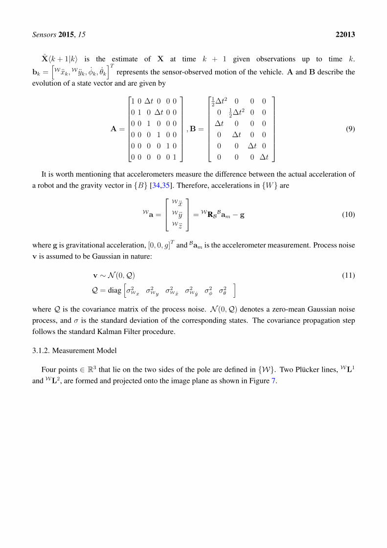
X〈k + 1|k〉 is the estimate of X at time k + 1 given observations up to time k.

bk =[W xk,

W yk, φk, θk

]Trepresents the sensor-observed motion of the vehicle. A and B describe the

evolution of a state vector and are given by

A =

1 0 ∆t 0 0 0

0 1 0 ∆t 0 0

0 0 1 0 0 0

0 0 0 1 0 0

0 0 0 0 1 0

0 0 0 0 0 1

,B =

12∆t2 0 0 0

0 12∆t2 0 0

∆t 0 0 0

0 ∆t 0 0

0 0 ∆t 0

0 0 0 ∆t

(9)

It is worth mentioning that accelerometers measure the difference between the actual acceleration ofa robot and the gravity vector in {B} [34,35]. Therefore, accelerations in {W} are

Wa =

W xW yW z

= WRBBam − g (10)

where g is gravitational acceleration, [0, 0, g]T and Bam is the accelerometer measurement. Process noisev is assumed to be Gaussian in nature:

v ∼ N (0,Q) (11)

Q = diag[σ2

Wx σ2Wy σ2

W x σ2W y σ2

φ σ2θ

]

where Q is the covariance matrix of the process noise. N (0,Q) denotes a zero-mean Gaussian noiseprocess, and σ is the standard deviation of the corresponding states. The covariance propagation stepfollows the standard Kalman Filter procedure.

3.1.2. Measurement Model

Four points ∈ R3 that lie on the two sides of the pole are defined in {W}. Two Plücker lines, WL1

and WL2, are formed and projected onto the image plane as shown in Figure 7.

Sensors 2015, 15 22014

y

xz

WA

WB

WC

WD

yxz

r

WL1

WL2

{Ck}{Ck+1}

`1k

`2k

ak

bk

ck

ck+1

dk+1

dk

ak+1

bk+1

Figure 7. Projection model for a cylindrical object. WA,WB,WC,WD ∈ R3 denote pointsin the world frame with ak, bk, ck, dk ∈ R2 denoting their corresponding projection onto aplanar imaging surface at a sample k. Although we actually measure different world pointsbetween frames, they are considered to be the same point due to the cylindrical nature of theobject and the choice of line representation.

We partition the measurement into two components: visual zcam and inertial zIMU. The measurementvector is

Zk =

`1k`2kφk

θk

=

[zcam

zIMU

](12)

where `ik ∈ R2 are the 2D line features from the tracker as given by Equation (5). The projected lineobservation is given by the nonlinear function of Equation (3)

zcam =

[hcam(WL1,W xk,

W yk, φk, θk,w)

hcam(WL2,W xk,W yk, φk, θk,w)

](13)

=

[C(W xk,

W yk, φk, θk)WL1C(W xk,

W yk, φk, θk)T

C(W xk,W yk, φk, θk)

WL2C(W xk,W yk, φk, θk)

T

](14)

Note that the unobservable states Wzk and ψ are omitted. w is the measurement noise withmeasurement covariance matrix,R

w ∼ N (0,R) (15)

R = diag[σ2α1 σ2

β1 σ2α2 σ2

β2 σ2φ σ2

θ

]

Sensors 2015, 15 22015

We manually tune these parameters by comparing the filter output with Vicon ground truth. Wegenerated the run-time code for Equation (14) using the MATLAB Symbolic Toolbox and then exportingthe C++ code. This model is 19 K lines of source code but computation time is just 6µs.

The update step for the filter requires linearization of this line model and evaluation of thetwo Jacobians

Hx =∂hcam

∂x|X(k), Hw =

∂hcam

∂w(16)

where Hx is a function of state that includes the camera projection model. We again use the MATLABSymbolic Toolbox and automatic code generation (58 K lines of source code) for Hx. It takes 30µs tocompute in the C++ implementation with the onboard CPU quad-core ARM Cortex-A9.

The remaining observations are the vehicle attitude, directly measured by the onboard IMU (zIMU) andreported at 100 Hz over a serial link. The linear observation model for the attitude is

zIMU =

[φk

θk

]= HIMU

WX (17)

HIMU =

[0 0 0 1 0 0

0 0 0 0 1 0

](18)

The measurements zcam and zIMU are available at 60 Hz and 100 Hz respectively. The EKF issynchronous with the 60 Hz vision data and the most recent zIMU measurement is used for the filterupdate. Inputs and outputs of the horizontal plane EKF are presented in Figure 5.

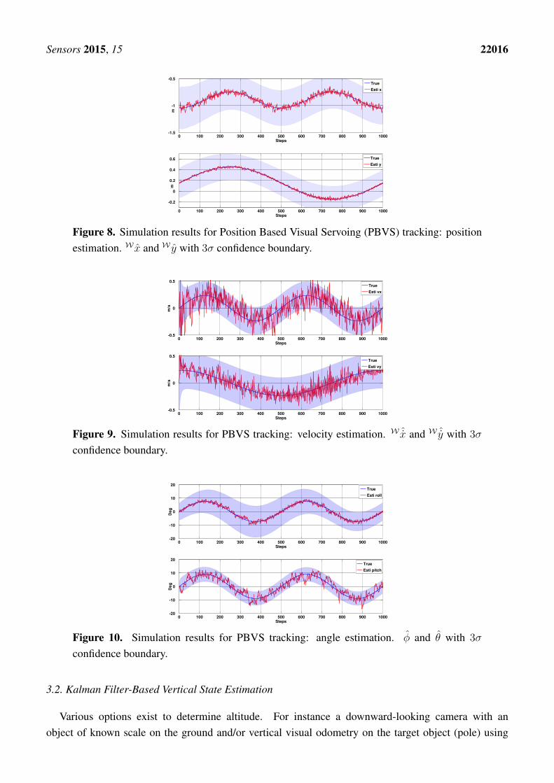
3.1.3. Simulation Results

In order to validate the EKF line model and Jacobian, we create a virtual camera observing four points,Pi ∈ R3 and move the camera with sinusoidal motion in 4 DOF (Wx,Wy, φ, θ) using the simulationframework of [36]. To emulate the errors in line measurements we set the measurement uncertainties tobe σα = 1◦ and σβ = 4 pixels in the line parameters, α and β, from Equation (5). Estimation results, theirconfidence boundary and noise parameters are shown in Figures 8–10. Most of the states are within 3σ

confidence level. The total simulation time is 10 s, with a sampling rate of 100 Hz. We see good qualityestimates of position and velocity in the horizontal plane, whilst decoupling the effects of attitude onthe projected line parameters. We see that the x-axis forward estimation is noisier than the y-axis sinceimage variation due to change in camera depth is much less than that due to fronto-parallel motion.

Sensors 2015, 15 22016

Steps

m

0 100 200 300 400 500 600 700 800 900 1000-1.5

-1

-0.5TrueEsti x

Steps

m

0 100 200 300 400 500 600 700 800 900 1000

-0.2

0

0.2

0.4

0.6 TrueEsti y

Figure 8. Simulation results for Position Based Visual Servoing (PBVS) tracking: positionestimation. W x and W y with 3σ confidence boundary.

Steps

m/s

0 100 200 300 400 500 600 700 800 900 1000-0.5

0

0.5TrueEsti vx

Steps

m/s

0 100 200 300 400 500 600 700 800 900 1000-0.5

0

0.5TrueEsti vy

Figure 9. Simulation results for PBVS tracking: velocity estimation. W ˆx and W ˆy with 3σ

confidence boundary.

Steps

Deg

0 100 200 300 400 500 600 700 800 900 1000-20

-10

0

10

20TrueEsti roll

Steps

Deg

0 100 200 300 400 500 600 700 800 900 1000-20

-10

0

10

20TrueEsti pitch

Figure 10. Simulation results for PBVS tracking: angle estimation. φ and θ with 3σ

confidence boundary.

3.2. Kalman Filter-Based Vertical State Estimation

Various options exist to determine altitude. For instance a downward-looking camera with anobject of known scale on the ground and/or vertical visual odometry on the target object (pole) using

Sensors 2015, 15 22017

the forward-facing camera. Due to onboard computational limits we opt, at this stage, to use asonar altimeter. We observe altitude directly using a downward-facing ultrasonic sensor at 20 Hz,but this update rate is too low for control purposes and any derived velocity signal has too much lag.Therefore we use another Kalman Filter to fuse this with the 100 Hz inertial data which includes verticalacceleration in {B}. The sonar sensor is calibrated by least square fitting to ground truth state estimates.The altitude and z-axis acceleration measurement in {B} are transformed to {W} using φ and θ anglesand Equation (10). WXalt is the vertical state,

[Wz,W z]T and the process model is given by

WXalt〈k+1|k〉 =Aalt

[W z〈k|k〉W ˆz〈k|k〉

]+ BaltW z + valt (19)

where

Aalt =

[1 ∆t

0 1

], Balt =

[12∆t2

∆t

](20)

and where valt is the process noise vector of Wz and W z. The covariance matrices of the process andmeasurement noise, Qalt and Ralt, are defined as Equations (12) and (16). The observation matrix isHalt =

[1 0

].

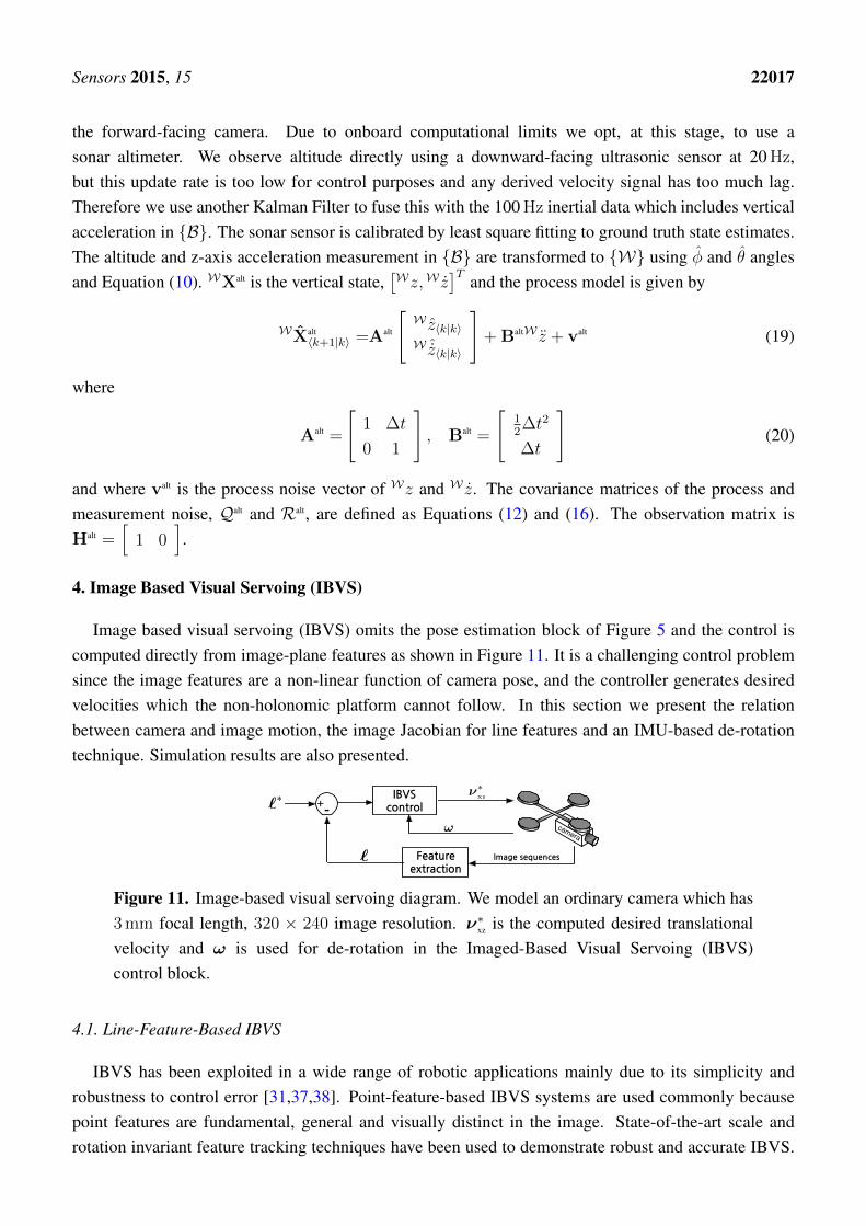
4. Image Based Visual Servoing (IBVS)

Image based visual servoing (IBVS) omits the pose estimation block of Figure 5 and the control iscomputed directly from image-plane features as shown in Figure 11. It is a challenging control problemsince the image features are a non-linear function of camera pose, and the controller generates desiredvelocities which the non-holonomic platform cannot follow. In this section we present the relationbetween camera and image motion, the image Jacobian for line features and an IMU-based de-rotationtechnique. Simulation results are also presented.

Featureextraction

IBVScontrol

Image����������� ������������������  sequences

-+camera

`

`⇤

!

⌫⇤xz

Figure 11. Image-based visual servoing diagram. We model an ordinary camera which has3 mm focal length, 320 × 240 image resolution. ν∗xz is the computed desired translationalvelocity and ω is used for de-rotation in the Imaged-Based Visual Servoing (IBVS)control block.

4.1. Line-Feature-Based IBVS

IBVS has been exploited in a wide range of robotic applications mainly due to its simplicity androbustness to control error [31,37,38]. Point-feature-based IBVS systems are used commonly becausepoint features are fundamental, general and visually distinct in the image. State-of-the-art scale androtation invariant feature tracking techniques have been used to demonstrate robust and accurate IBVS.

Sensors 2015, 15 22018

By comparison line-feature-based IBVS implementations are relatively rare, yet lines are distinctvisual features in man-made environments, for examples the edges of roads, buildings and powerdistribution poles.

4.1.1. Image Jacobian for Line Features

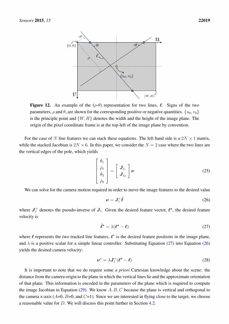
The homogeneous equation of a 2D line is au + bv + c = 0 with coefficients (a, b, c). Although anyline can be represented in this form it does not have a minimum number of parameters. The standardslope-intercept form v = mu + c where m is slope and c is intercept is problematic for the case ofvertical lines where m = ∞. We therefore choose (ρ, θ) parameterization as the 2D line representationas shown in Figure 12

u sin θ + v cos θ = ρ (21)

where θ ∈ [−π2, π2) is the angle from the u-axis to v-axis in radians, and ρ ∈ [−ρmin, ρmax] is the

perpendicular distance in pixels from the origin to the line. This form can represent a horizontal line(θ = 0) and a vertical line (θ = −π

2).

For a moving camera, the rate of change of line parameters is related to the camera velocity by

˙ =

[θ

ρ

]= J lν (22)

where θ and ρ are the velocity of a line feature, and are analogous to optical flow for a point feature.These line parameters are simply related to the line parameters introduced earlier by

θ = tan−1 α, ρ = β cos θ (23)

The matrix Jl is the Image Jacobian or Interaction matrix and given by Equation (29) [39]. The lineslie on the equation of a plane AX +BY +CZ +D = 0 where (A,B,C) is the plane normal vector andD is the distance between the plane and the camera. The camera spatial velocity in world coordinates is

ν =[vx, vy, vz | ωx, ωy, ωz

]T(24)

=[νt | ω

]T

where νt and ω are the translational and angular velocity components respectively.

Sensors 2015, 15 22019

u

v

{0, 0}

{u0, v0}

`

{W, H}

_

_

Figure 12. An example of the (ρ-θ) representation for two lines, `. Signs of the twoparameters, ρ and θ, are shown for the corresponding positive or negative quantities. {u0, v0}is the principle point and {W,H} denotes the width and the height of the image plane. Theorigin of the pixel coordinate frame is at the top-left of the image plane by convention.

For the case of N line features we can stack these equations. The left hand side is a 2N × 1 matrix,while the stacked Jacobian is 2N × 6. In this paper, we consider the N = 2 case where the two lines arethe vertical edges of the pole, which yields

θ1

ρ1

θ2

ρ2

=

[J l1J l2

]ν (25)

We can solve for the camera motion required in order to move the image features to the desired value

ν = J+l˙ (26)

where J+l denotes the pseudo-inverse of J l. Given the desired feature vector, `∗, the desired feature

velocity is

˙∗ = λ(`∗ − `) (27)

where ` represents the two tracked line features, `∗ is the desired feature positions in the image plane,and λ is a positive scalar for a simple linear controller. Substituting Equation (27) into Equation (26)yields the desired camera velocity:

ν∗ = λJ+l (`∗ − `) (28)

It is important to note that we do require some a priori Cartesian knowledge about the scene: thedistance from the camera origin to the plane in which the vertical lines lie and the approximate orientationof that plane. This information is encoded in the parameters of the plane which is required to computethe image Jacobian in Equation (29). We know A,B,C because the plane is vertical and orthogonal tothe camera x-axis (A=0, B=0, and C=1). Since we are interested in flying close to the target, we choosea reasonable value for D. We will discuss this point further in Section 4.2.

Sensors 2015, 15 22020

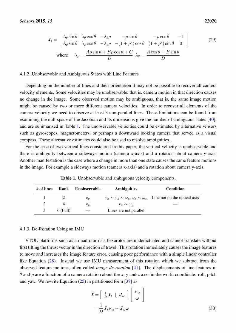
J l =

[λθ sin θ λθ cos θ −λθρ −ρ sin θ −ρ cos θ −1

λρ sin θ λρ cos θ −λρρ −(1 + ρ2) cos θ (1 + ρ2) sin θ 0

](29)

where λρ =Aρ sin θ +Bρ cos θ + C

D, λθ =

A cos θ −B sin θ

D

4.1.2. Unobservable and Ambiguous States with Line Features

Depending on the number of lines and their orientation it may not be possible to recover all cameravelocity elements. Some velocities may be unobservable, that is, camera motion in that direction causesno change in the image. Some observed motion may be ambiguous, that is, the same image motionmight be caused by two or more different camera velocities. In order to recover all elements of thecamera velocity we need to observe at least 3 non-parallel lines. These limitations can be found fromexamining the null-space of the Jacobian and its dimensions give the number of ambiguous states [40],and are summarised in Table 1. The unobservable velocities could be estimated by alternative sensorssuch as gyroscopes, magnetometers, or perhaps a downward looking camera that served as a visualcompass. These alternative estimates could also be used to resolve ambiguities.

For the case of two vertical lines considered in this paper, the vertical velocity is unobservable andthere is ambiguity between a sideways motion (camera x-axis) and a rotation about camera y-axis.Another manifestation is the case where a change in more than one state causes the same feature motionsin the image. For example a sideways motion (camera x-axis) and a rotation about camera y-axis.

Table 1. Unobservable and ambiguous velocity components.

# of lines Rank Unobservable Ambiguities Condition

1 2 vy vx ∼ vz ∼ ωy, ωx ∼ ωz Line not on the optical axis2 4 vy vx ∼ ωy —3 6 (Full) — Lines are not parallel

4.1.3. De-Rotation Using an IMU

VTOL platforms such as a quadrotor or a hexarotor are underactuated and cannot translate withoutfirst tilting the thrust vector in the direction of travel. This rotation immediately causes the image featuresto move and increases the image feature error, causing poor performance with a simple linear controllerlike Equation (28). Instead we use IMU measurement of this rotation which we subtract from theobserved feature motions, often called image de-rotation [41]. The displacements of line features inθ and ρ are a function of a camera rotation about the x, y and z axes in the world coordinate: roll, pitchand yaw. We rewrite Equation (25) in partitioned form [37] as

˙ =[

1DJ t | Jω

] [ νxz

ω

]

=1

DJ tνxz + Jωω (30)

Sensors 2015, 15 22021

where ˙ is a 4 × 1 optical flow component, 1DJ t and Jω are 4 × 2 translational and 4 × 3 rotational

components. They are respectively columns {1, 3} and {4, 5, 6} of the stacked Jacobian,[J l1 ,J l2

]T.

Note we omit column {2} which corresponds to the unobservable state, vy. The reduced Jacobian isslightly better conditioned (smaller condition number) and the mean computation time is measuredat 30µs which is 20µs faster than for the full size Jacobian. Thus νxz contains only two elements,[vx, vz

]T, the translational camera velocity in the horizontal plane. This is input to the vehicle’s

roll and pitch angle control loops. The common denominator, D, denotes target object depth which isassumed, and ω is obtained from an IMU. We rearrange Equation (30) as

νxz = DJ+t ( ˙− Jωω) (31)

and we substitute Equation (27) into Equation (31) to write

ν∗xz = DJ+t (λ(`∗ − `)− Jωω︸︷︷︸) (32)

The de-rotation term is indicated, and subtracts the effect of camera rotation from the observedfeatures. After subtraction, only the desired translational velocity remains.

0 20 40 60 80 100−0.16

−0.14

−0.12

−0.1

−0.08

−0.06

−0.04

−0.02

0

0.02

Time(s)

Velo

city

(m/s

)

Vehicle translational velocity with derotation

xyz

(a)

0 20 40 60 80 100−0.16

−0.14

−0.12

−0.1

−0.08

−0.06

−0.04

−0.02

0

0.02

Time(s)

Velo

city

(m/s

)

Vehicle translational velocity w/o derotation

xyz

(b)

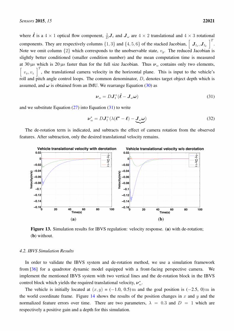
Figure 13. Simulation results for IBVS regulation: velocity response. (a) with de-rotation;(b) without.

4.2. IBVS Simulation Results

In order to validate the IBVS system and de-rotation method, we use a simulation frameworkfrom [36] for a quadrotor dynamic model equipped with a front-facing perspective camera. Weimplement the mentioned IBVS system with two vertical lines and the de-rotation block in the IBVScontrol block which yields the required translational velocity, ν∗xz.

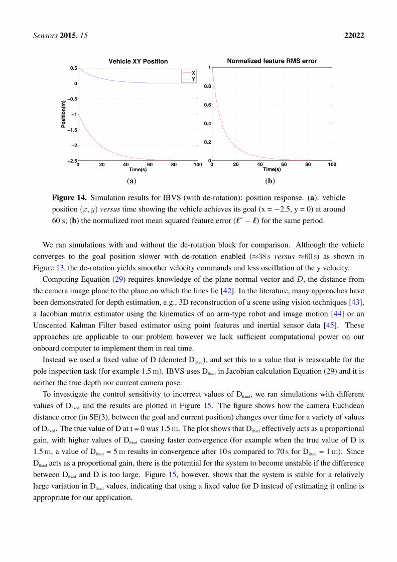
The vehicle is initially located at (x, y) = (−1.0, 0.5) m and the goal position is (−2.5, 0) m inthe world coordinate frame. Figure 14 shows the results of the position changes in x and y and thenormalized feature errors over time. There are two parameters, λ = 0.3 and D = 1 which arerespectively a positive gain and a depth for this simulation.

Sensors 2015, 15 22022

0 20 40 60 80 100−2.5

−2

−1.5

−1

−0.5

0

0.5

Time(s)

Posi

tion(

m)

Vehicle XY Position

XY

(a)

0 20 40 60 80 1000

0.2

0.4

0.6

0.8

1

Time(s)

Normalized feature RMS error

(b)

Figure 14. Simulation results for IBVS (with de-rotation): position response. (a): vehicleposition (x, y) versus time showing the vehicle achieves its goal (x = −2.5, y = 0) at around60 s; (b) the normalized root mean squared feature error (`∗ − `) for the same period.

We ran simulations with and without the de-rotation block for comparison. Although the vehicleconverges to the goal position slower with de-rotation enabled (≈38 s versus ≈60 s) as shown inFigure 13, the de-rotation yields smoother velocity commands and less oscillation of the y velocity.

Computing Equation (29) requires knowledge of the plane normal vector and D, the distance fromthe camera image plane to the plane on which the lines lie [42]. In the literature, many approaches havebeen demonstrated for depth estimation, e.g., 3D reconstruction of a scene using vision techniques [43],a Jacobian matrix estimator using the kinematics of an arm-type robot and image motion [44] or anUnscented Kalman Filter based estimator using point features and inertial sensor data [45]. Theseapproaches are applicable to our problem however we lack sufficient computational power on ouronboard computer to implement them in real time.

Instead we used a fixed value of D (denoted Dfixed), and set this to a value that is reasonable for thepole inspection task (for example 1.5 m). IBVS uses Dfixed in Jacobian calculation Equation (29) and it isneither the true depth nor current camera pose.

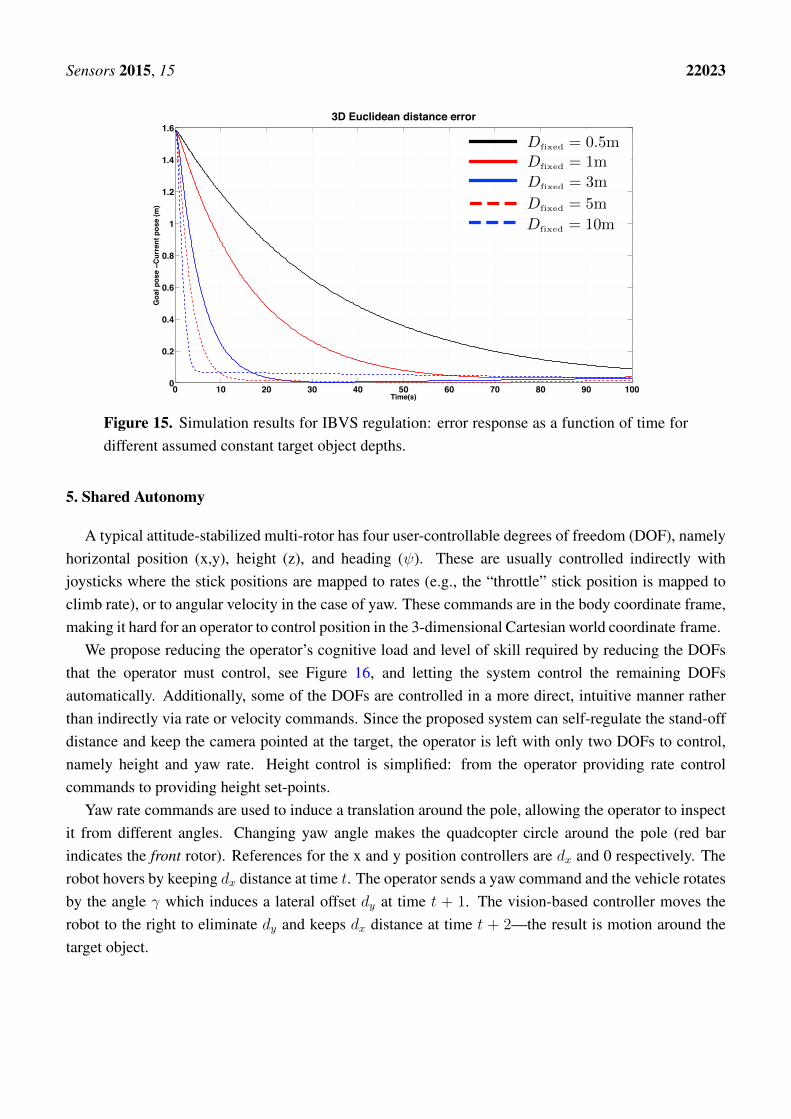
To investigate the control sensitivity to incorrect values of Dfixed, we ran simulations with differentvalues of Dfixed and the results are plotted in Figure 15. The figure shows how the camera Euclideandistance error (in SE(3), between the goal and current position) changes over time for a variety of valuesof Dfixed. The true value of D at t = 0 was 1.5 m. The plot shows that Dfixed effectively acts as a proportionalgain, with higher values of Dfixed causing faster convergence (for example when the true value of D is1.5 m, a value of Dfixed = 5 m results in convergence after 10 s compared to 70 s for Dfixed = 1 m). SinceDfixed acts as a proportional gain, there is the potential for the system to become unstable if the differencebetween Dfixed and D is too large. Figure 15, however, shows that the system is stable for a relativelylarge variation in Dfixed values, indicating that using a fixed value for D instead of estimating it online isappropriate for our application.

Sensors 2015, 15 22023

0 10 20 30 40 50 60 70 80 90 1000

0.2

0.4

0.6

0.8

1

1.2

1.4

1.6

Time(s)

Goa

l pos

e −C

urre

nt p

ose

(m)

3D Euclidean distance error

D=0.5mD=1mD=3mD=5mD=10m

Dfixed = 0.5m

Dfixed = 1m

Dfixed = 3m

Dfixed = 5m

Dfixed = 10m

Dfixed = 0.5mDfixed = 1m

Dfixed = 3m

Dfixed = 5m

Dfixed = 10m

Figure 15. Simulation results for IBVS regulation: error response as a function of time fordifferent assumed constant target object depths.

5. Shared Autonomy

A typical attitude-stabilized multi-rotor has four user-controllable degrees of freedom (DOF), namelyhorizontal position (x,y), height (z), and heading (ψ). These are usually controlled indirectly withjoysticks where the stick positions are mapped to rates (e.g., the “throttle” stick position is mapped toclimb rate), or to angular velocity in the case of yaw. These commands are in the body coordinate frame,making it hard for an operator to control position in the 3-dimensional Cartesian world coordinate frame.

We propose reducing the operator’s cognitive load and level of skill required by reducing the DOFsthat the operator must control, see Figure 16, and letting the system control the remaining DOFsautomatically. Additionally, some of the DOFs are controlled in a more direct, intuitive manner ratherthan indirectly via rate or velocity commands. Since the proposed system can self-regulate the stand-offdistance and keep the camera pointed at the target, the operator is left with only two DOFs to control,namely height and yaw rate. Height control is simplified: from the operator providing rate controlcommands to providing height set-points.

Yaw rate commands are used to induce a translation around the pole, allowing the operator to inspectit from different angles. Changing yaw angle makes the quadcopter circle around the pole (red barindicates the front rotor). References for the x and y position controllers are dx and 0 respectively. Therobot hovers by keeping dx distance at time t. The operator sends a yaw command and the vehicle rotatesby the angle γ which induces a lateral offset dy at time t + 1. The vision-based controller moves therobot to the right to eliminate dy and keeps dx distance at time t + 2—the result is motion around thetarget object.

Sensors 2015, 15 22024

Pole center

dx

dy

�

dx

Time = t Time = t + 1 Time = t + 2

Top views Constrained motion

Figure 16. (left) illustration of how vehicle induces yaw motion. γ is an angle forthe yaw motion and dx and dy are distances between the pole and the robot in x-, andy-axis; (right) reduced dimension task space for operator commands which is sufficient forinspection purposes.

6. Experimental Results

The experiments we present are summarised in Figure 17 and can be considered with respect to manycategories: autonomous or manual, PBVS or IBVS control, hovering or circumnavigation, indoor oroutdoor, day or night. The manual pilot experiments pit two human pilots, with different skill levels,against the autonomous system for the tasks of hovering and circumnavigation. Figure 18 shows somesample images from the onboard front-camera captured during various experiments. The demonstrationvideo is available from the following link [22].

PBVS

Indoor

Day Night

Outdoor

Hovering- Control performance- State estimation (position and velocity) performance

Circum-navigation- Control performance- 3D trajectory plot

Autonomous flying experiments Manual pilot experiments

Day

Outdoor

1 2

Hovering- Control performance- State estimation (position and velocity) performance

Hovering- Control performance- State estimation (position and velocity) performance

IBVS

Indoor

Day Night

Outdoor

Hovering- Control performance- Feature errors and desired velocity Circum-navigation

- Control performance- 3D trajectory plot

Hovering- Control performance- Feature errors and desired velocity

Hovering- Control performance- Feature errors and desired velocity

Hovering- Control performance

Circum-navigation- Control performance- 3D trajectory plot

Figure 17. Overview of experiments. There are two categories: autonomous flyingwith shared autonomy (left) and manual piloting with only attitude stabilization (right);Autonomous flying consists of PBVS (top) and IBVS (bottom). Two pilots were involved inthe manual piloting experiments. Each box with grey denotes a sub-experiment and describeskey characteristics of that experiment.

Sensors 2015, 15 22025

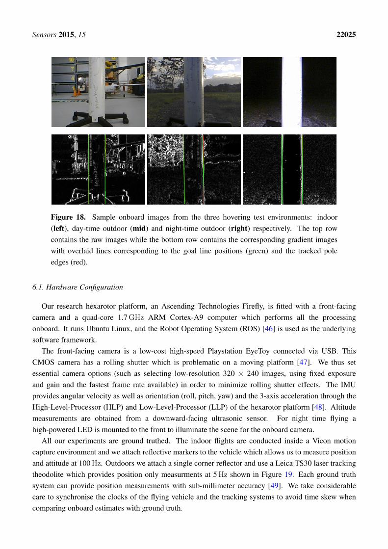
Figure 18. Sample onboard images from the three hovering test environments: indoor(left), day-time outdoor (mid) and night-time outdoor (right) respectively. The top rowcontains the raw images while the bottom row contains the corresponding gradient imageswith overlaid lines corresponding to the goal line positions (green) and the tracked poleedges (red).

6.1. Hardware Configuration

Our research hexarotor platform, an Ascending Technologies Firefly, is fitted with a front-facingcamera and a quad-core 1.7 GHz ARM Cortex-A9 computer which performs all the processingonboard. It runs Ubuntu Linux, and the Robot Operating System (ROS) [46] is used as the underlyingsoftware framework.

The front-facing camera is a low-cost high-speed Playstation EyeToy connected via USB. ThisCMOS camera has a rolling shutter which is problematic on a moving platform [47]. We thus setessential camera options (such as selecting low-resolution 320 × 240 images, using fixed exposureand gain and the fastest frame rate available) in order to minimize rolling shutter effects. The IMUprovides angular velocity as well as orientation (roll, pitch, yaw) and the 3-axis acceleration through theHigh-Level-Processor (HLP) and Low-Level-Processor (LLP) of the hexarotor platform [48]. Altitudemeasurements are obtained from a downward-facing ultrasonic sensor. For night time flying ahigh-powered LED is mounted to the front to illuminate the scene for the onboard camera.

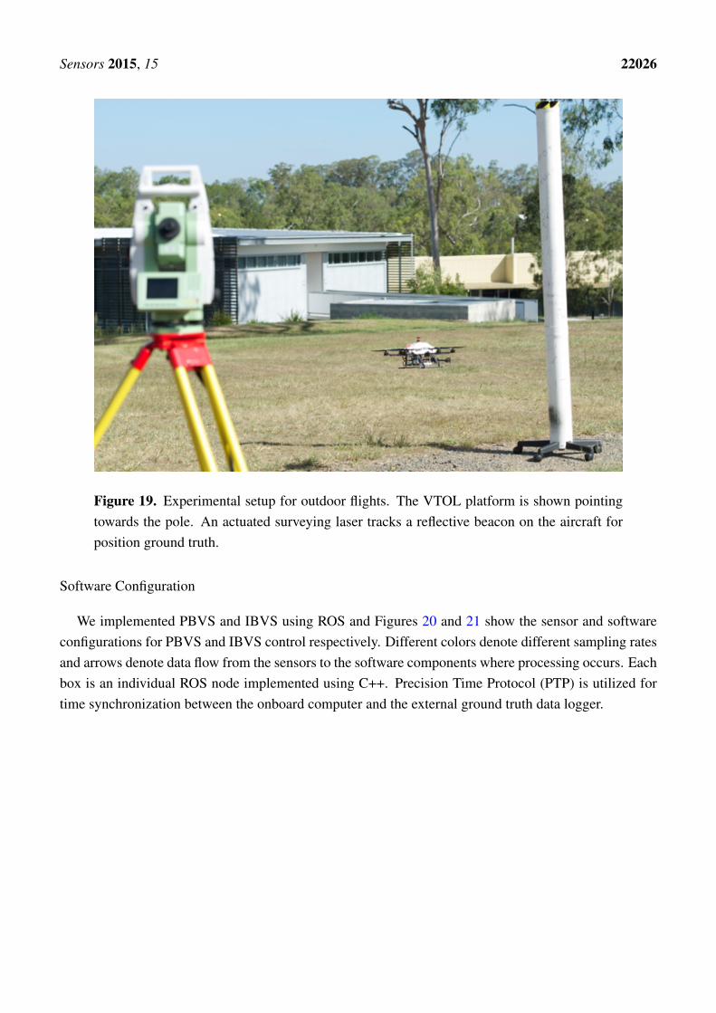
All our experiments are ground truthed. The indoor flights are conducted inside a Vicon motioncapture environment and we attach reflective markers to the vehicle which allows us to measure positionand attitude at 100 Hz. Outdoors we attach a single corner reflector and use a Leica TS30 laser trackingtheodolite which provides position only measurments at 5 Hz shown in Figure 19. Each ground truthsystem can provide position measurements with sub-millimeter accuracy [49]. We take considerablecare to synchronise the clocks of the flying vehicle and the tracking systems to avoid time skew whencomparing onboard estimates with ground truth.

Sensors 2015, 15 22026

Figure 19. Experimental setup for outdoor flights. The VTOL platform is shown pointingtowards the pole. An actuated surveying laser tracks a reflective beacon on the aircraft forposition ground truth.

Software Configuration

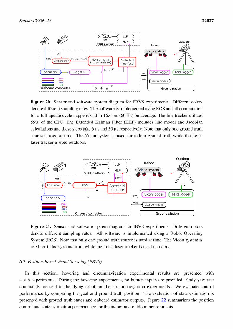
We implemented PBVS and IBVS using ROS and Figures 20 and 21 show the sensor and softwareconfigurations for PBVS and IBVS control respectively. Different colors denote different sampling ratesand arrows denote data flow from the sensors to the software components where processing occurs. Eachbox is an individual ROS node implemented using C++. Precision Time Protocol (PTP) is utilized fortime synchronization between the onboard computer and the external ground truth data logger.

Sensors 2015, 15 22027

Line tracker

Onboard computer

EKF estimator(PBVS pose estimator)

Sonar

Sonar drv

USB

�1,⇥1,�2,⇥2

⇥� � a

⇤T

Height KF

Camera

Ground station

PTPVicon logger

User commandWiFi

HLPIMU

LLP

VTOL platform

60Hz20Hz5Hz

100Hz

Asctech hl interface

[z z]T

Laser

Leica logger

tracker

IndoorOutdoor

RS232

Figure 20. Sensor and software system diagram for PBVS experiments. Different colorsdenote different sampling rates. The software is implemented using ROS and all computationfor a full update cycle happens within 16.6 ms (60 Hz) on average. The line tracker utilizes55% of the CPU. The Extended Kalman Filter (EKF) includes line model and Jacobiancalculations and these steps take 6µs and 30µs respectively. Note that only one ground truthsource is used at time. The Vicon system is used for indoor ground truth while the Leicalaser tracker is used outdoors.

Line tracker

HLP

Asctech hl interface

Onboard computer

IBVS

USB

60Hz20Hz

Sonar drv

Camera

IMU

5Hz

RS232 `1, `2

!

z

RS232

LLP

VTOL platform

⌫⇤xz

100Hz

Ground station

PTPVicon logger

User commandWiFi

Laser

Leica logger

tracker

IndoorOutdoor

Figure 21. Sensor and software system diagram for IBVS experiments. Different colorsdenote different sampling rates. All software is implemented using a Robot OperatingSystem (ROS). Note that only one ground truth source is used at time. The Vicon system isused for indoor ground truth while the Leica laser tracker is used outdoors.

6.2. Position-Based Visual Servoing (PBVS)

In this section, hovering and circumnavigation experimental results are presented with4 sub-experiments. During the hovering experiments, no human inputs are provided. Only yaw ratecommands are sent to the flying robot for the circumnavigation experiments. We evaluate controlperformance by comparing the goal and ground truth position. The evaluation of state estimation ispresented with ground truth states and onboard estimator outputs. Figure 22 summarizes the positioncontrol and state estimation performance for the indoor and outdoor environments.

Sensors 2015, 15 22028

Indoor Outdoor (day)

Outdoor (night) Indoor Outdoor

(day)Outdoor (night)

0.048 0.038 0.047 0.016 0.019 0.019 m

0.024 0.028 0.043 0.01 0.024 0.03 m

0.011 0.022 0.016 0.008 0.015 0.013 m___ ___ ___ 0.038 0.12 0.152 m/s___ ___ ___ 0.015 0.053 0.108 m/s___ ___ ___ 0.042 0.04 0.031 m/s___ ___ ___ 0.294 ___ ___ deg___ ___ ___ 1.25 ___ ___ deg

Time interval 15~55 10~50 10~50 15~55 10~50 10~50 s

Control performance State estimator performanceState Unit

!x!y

!zφ

θ

xyz

Figure 22. PBVS hovering (standard deviation).

6.2.1. PBVS Indoor Hovering

The control performance is evaluated by computing the standard deviation of the error between thegoal position (x, y and z) and ground truth as measured by the Vicon system. The performance of thecontroller is shown in Figure 23. Interestingly, although the x-axis velocity estimation is noisy, thecontrol performance for this axis is not significantly worse than for the y-axis, the quadrotor plant iseffectively filtering out this noise.

0 10 20 30 40 50 60 70−1

−0.8

−0.6

−0.4The desired goal x∗ and ground truth x

Posi

tion

x (m

)

Time(s)

Vicon xx∗

0 10 20 30 40 50 60 70

−0.2−0.1

00.10.2

The desired goal y∗ and ground truth y

Posi

tion

y (m

)

Time(s)

Vicon yy∗

0 10 20 30 40 50 60 700.4

0.6

0.8

1The desired goal z ∗ and ground truth z

Posi

tion

z (m

)

Time(s)

Vicon zz ∗

Figure 23. Experimental results for PBVS-based indoor hovering: control performance.Goal (black) and ground truth states (blue). The desired position for W x, W y and W z is−0.7 m, 0 m and 0.7 m. We compute standard deviation of errors for each state over theinterval 15 s∼63 s: σx = 0.048 m, σy = 0.024 m, and σz = 0.011 m.

Sensors 2015, 15 22029

0 10 20 30 40 50 60 70−0.8

−0.6

−0.4x and ground truth x

Time(s)

Posi

tion

x (m

)

Vicon xx

0 10 20 30 40 50 60 70−0.2

0

0.2y and ground truth y

Posi

tion

y (m

)

Time(s)

Vicon yy

0 10 20 30 40 50 60 700.4

0.5

0.6

0.7

z and ground truth z

Posi

tion

z (m

)

Time(s)

Vicon zz

(a)

0 10 20 30 40 50 60 70−0.2

−0.1

0

0.1

0.2vx and ground truth vx

Time(s)

Velo

city

(m/s

)

Vicon vxvx

0 10 20 30 40 50 60 70−0.2

−0.1

0

0.1

0.2vy and ground truth vy

Time(s)

Velo

city

(m/s

)

Vicon vyvy

0 10 20 30 40 50 60 70−0.2

−0.1

0

0.1

0.2vz and ground truth vz

Time(s)

Velo

city

(m/s

)

Vicon vzvz

(b)

0 10 20 30 40 50 60 70−5

0

5φ and ground truth φ

Time(s)

Deg

Vicon φφ

0 10 20 30 40 50 60 70−5

0

5θ and ground truth θ

Time(s)

Deg

Vicon θθ

(c)

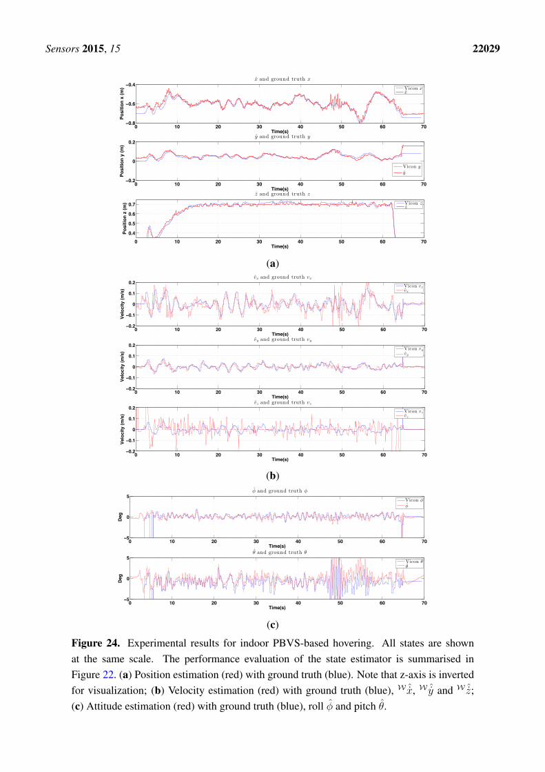
Figure 24. Experimental results for indoor PBVS-based hovering. All states are shownat the same scale. The performance evaluation of the state estimator is summarised inFigure 22. (a) Position estimation (red) with ground truth (blue). Note that z-axis is invertedfor visualization; (b) Velocity estimation (red) with ground truth (blue), W ˆx, W ˆy and W ˆz;(c) Attitude estimation (red) with ground truth (blue), roll φ and pitch θ.

Sensors 2015, 15 22030

We estimate position and orientation except heading angle as shown in Figure 24. The robot oscillatesaround 48 s–50 s when the line tracker was affected by the noisy background leading to errors in theposition estimate W x.

0 5 10 15 20 25 30 35 40 45 50−1

−0.8

−0.6

Position ground truth from Leika

Time(s)

Posi

tion

x (m

)

Leica xx∗

0 5 10 15 20 25 30 35 40 45 50

−0.2−0.1

00.10.2

Time(s)

Posi

tion

y (m

)

Leica yy∗

0 5 10 15 20 25 30 35 40 45 500.4

0.6

0.8

1

Time(s)

Posi

tion

z (m

)

Leica zz ∗

Figure 25. Experimental results for outdoor (day) PBVS-based hovering: controlperformance. Goal (black) and ground truth states (blue) . The desired position for W x,W y and W z is −0.7 m, 0 m and 0.7 m. We compute standard deviations of errors for eachstate over the interval 10 s∼50 s: σx = 0.038 m, σy = 0.028 m, and σz = 0.022 m.

6.2.2. PBVS Day-Time Outdoor Hovering

The VTOL platform was flown outdoors where external disturbances such as wind gusts areencountered. In addition, background scenes were nosier as shown in Figure 18. Figures 25 and 26show control performance and state estimation during day-time hovering outdoors. The proposed systemwas able to efficiently reject disturbances and maintain a fixed stand-off distance from a pole (seeaccompanying video demonstration 2.2). Position and velocity estimation results are shown in Figure 26and are noisier than for the indoor case due to more complex naturally textured background scenes (seeFigure 18). Controller performance is consistent with that observed indoors. All results are within a±0.02 m variation boundary.

Sensors 2015, 15 22031

0 5 10 15 20 25 30 35 40 45 50−1

−0.8

−0.6

x and ground truth x

Time(s)

Posi

tion

x (m

)

Leica xx

0 5 10 15 20 25 30 35 40 45 50

−0.2

0

0.2

y and ground truth y

Time(s)

Posi

tion

y (m

)

Leica yy

0 5 10 15 20 25 30 35 40 45 50

0.4

0.6

0.8z and ground truth z

Posi

tion

z (m

)

Time(s)

Leica zz

(a)

0 5 10 15 20 25 30 35 40 45 50−0.5

0

0.5Ground truth vx and vx

Time(s)

Velo

city

x (m

/s)

Leica vxvx

0 5 10 15 20 25 30 35 40 45 50−0.5

0

0.5Ground truth vy and vy

Time(s)

Velo

city

y (m

/s)

Leica vyvy

0 5 10 15 20 25 30 35 40 45 50−0.5

0

0.5Ground truth vz and vz

Time(s)

Velo

city

z (m

/s)

Leica vzvz

(b)

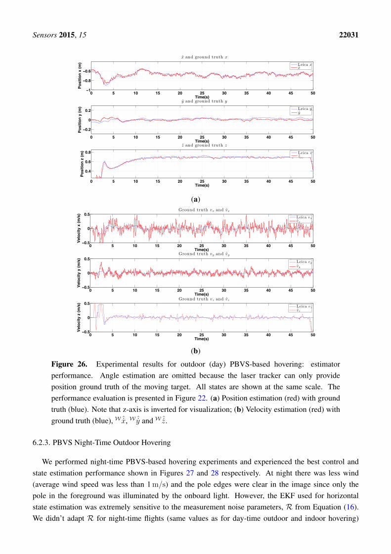
Figure 26. Experimental results for outdoor (day) PBVS-based hovering: estimatorperformance. Angle estimation are omitted because the laser tracker can only provideposition ground truth of the moving target. All states are shown at the same scale. Theperformance evaluation is presented in Figure 22. (a) Position estimation (red) with groundtruth (blue). Note that z-axis is inverted for visualization; (b) Velocity estimation (red) withground truth (blue), W ˆx, W ˆy and W ˆz.

6.2.3. PBVS Night-Time Outdoor Hovering

We performed night-time PBVS-based hovering experiments and experienced the best control andstate estimation performance shown in Figures 27 and 28 respectively. At night there was less wind(average wind speed was less than 1 m/s) and the pole edges were clear in the image since only thepole in the foreground was illuminated by the onboard light. However, the EKF used for horizontalstate estimation was extremely sensitive to the measurement noise parameters, R from Equation (16).We didn’t adapt R for night-time flights (same values as for day-time outdoor and indoor hovering)

Sensors 2015, 15 22032

and this led to poor state estimation and oscillation in the x and y-axes—the worst results amongthe 3 experiments. This is a potential limitation of the deterministic Extended Kalman Filter (FilterTuning). [50,51] exploited stochastic gradient descent in order to learn R with accurate ground truthsuch as motion capture or high quality GPS. We are interested in this adaptive online learning for filterframeworks; however, this is beyond the scope of this work.

0 5 10 15 20 25 30 35 40 45 50−1

−0.8

−0.6

Position ground truth from Leika

Time(s)

Posi

tion

x (m

)

Leica xx∗

0 5 10 15 20 25 30 35 40 45 50

−0.2−0.1

00.10.2

Time(s)

Posi

tion

y (m

)

Leica yy∗

0 5 10 15 20 25 30 35 40 45 500.4

0.6

0.8

1

Time(s)

Posi

tion

z (m

)

Leica zz ∗

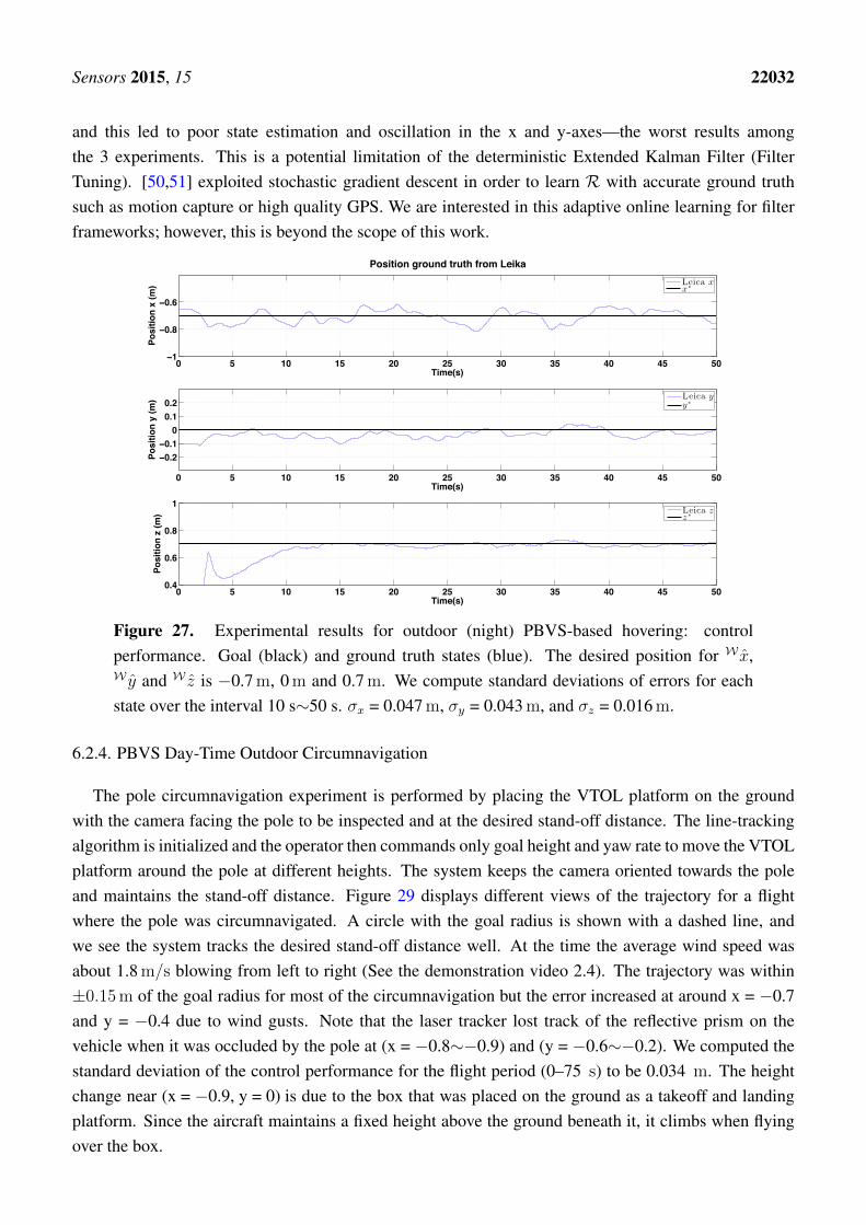
Figure 27. Experimental results for outdoor (night) PBVS-based hovering: controlperformance. Goal (black) and ground truth states (blue). The desired position for W x,W y and W z is −0.7 m, 0 m and 0.7 m. We compute standard deviations of errors for eachstate over the interval 10 s∼50 s. σx = 0.047 m, σy = 0.043 m, and σz = 0.016 m.

6.2.4. PBVS Day-Time Outdoor Circumnavigation

The pole circumnavigation experiment is performed by placing the VTOL platform on the groundwith the camera facing the pole to be inspected and at the desired stand-off distance. The line-trackingalgorithm is initialized and the operator then commands only goal height and yaw rate to move the VTOLplatform around the pole at different heights. The system keeps the camera oriented towards the poleand maintains the stand-off distance. Figure 29 displays different views of the trajectory for a flightwhere the pole was circumnavigated. A circle with the goal radius is shown with a dashed line, andwe see the system tracks the desired stand-off distance well. At the time the average wind speed wasabout 1.8 m/s blowing from left to right (See the demonstration video 2.4). The trajectory was within±0.15 m of the goal radius for most of the circumnavigation but the error increased at around x = −0.7and y = −0.4 due to wind gusts. Note that the laser tracker lost track of the reflective prism on thevehicle when it was occluded by the pole at (x = −0.8∼−0.9) and (y = −0.6∼−0.2). We computed thestandard deviation of the control performance for the flight period (0–75 s) to be 0.034 m. The heightchange near (x = −0.9, y = 0) is due to the box that was placed on the ground as a takeoff and landingplatform. Since the aircraft maintains a fixed height above the ground beneath it, it climbs when flyingover the box.

Sensors 2015, 15 22033

0 5 10 15 20 25 30 35 40 45 50−1

−0.8

−0.6

x and ground truth x

Time(s)

Posi

tion

x (m

)

Leica xx

0 5 10 15 20 25 30 35 40 45 50

−0.2−0.1

00.10.2

y and ground truth y

Time(s)

Posi

tion

y (m

)

Leica yy

0 5 10 15 20 25 30 35 40 45 50

0.4

0.6

0.8

z and ground truth z

Posi

tion

z (m

)

Time(s)

Leica zz

(a)

0 5 10 15 20 25 30 35 40 45 50−0.5

0

0.5Ground truth vx and vx

Time(s)

Velo

city

x (m

/s)

Leica vxvx

0 5 10 15 20 25 30 35 40 45 50−0.5

0

0.5Ground truth vy and vy

Time(s)

Velo

city

y (m

/s)

Leica vyvy

0 5 10 15 20 25 30 35 40 45 50−0.5

0

0.5Ground truth vz and vz

Time(s)

Velo

city

z (m

/s)

Leica vzvz

(b)

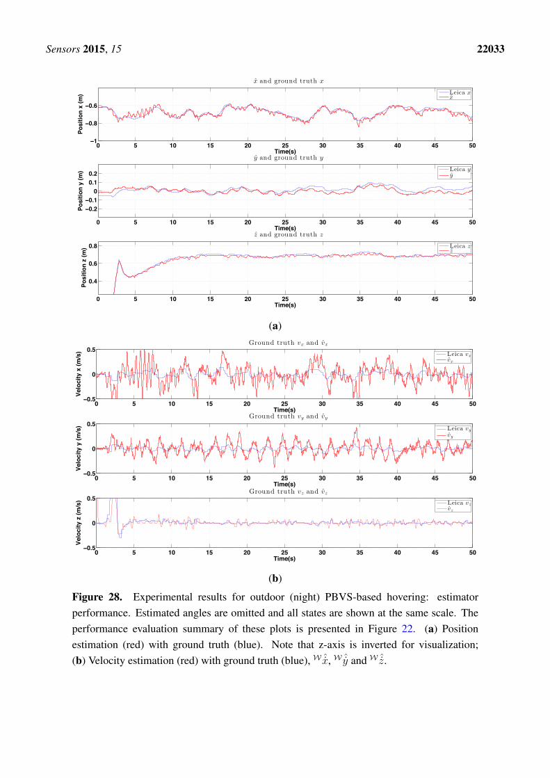
Figure 28. Experimental results for outdoor (night) PBVS-based hovering: estimatorperformance. Estimated angles are omitted and all states are shown at the same scale. Theperformance evaluation summary of these plots is presented in Figure 22. (a) Positionestimation (red) with ground truth (blue). Note that z-axis is inverted for visualization;(b) Velocity estimation (red) with ground truth (blue), W ˆx, W ˆy and W ˆz.

Sensors 2015, 15 22034

−0.8 −0.6 −0.4 −0.2 0 0.2 0.4 0.6 0.80

0.2

0.4

0.6

0.8

1

1.2

Ground truth trajectory during circumnavigating a target

x(m)

z(m

)

TrajectoryGoal

Pole centre

(a)

−0.8 −0.6 −0.4 −0.2 0 0.2 0.4 0.6 0.8

−0.5

0

0.5

0

0.2

0.4

0.6

0.8

1

1.2

y(m)

Ground truth trajectory during circumnavigating a target

x(m)

z(m

)

TrajectoryGoal

Pole centre

(b)

−0.8

−0.6

−0.4

−0.2

0

0.2

0.4

0.6

0.8

−0.8 −0.6 −0.4 −0.2 0 0.2 0.4 0.6 0.8

y(m)

Ground truth trajectory during circumnavigating a target

x(m

)

TrajectoryGoal

Pole centre

(c)

0 10 20 30 40 50 60 700

0.05

0.1

0.15

0.2

Time(s)

Goa

l pos

ition

− L

eica

pos

ition

(m)

Control performance error

(d)

Figure 29. Experimental results for outdoor (day) PBVS-based circumnavigation: controlperformance. (a–c) 3D views of the trajectory: Side view, Perspective view and Top view;(d) Euclidean error (goal minus actual) trajectory versus time.

6.3. Imaged-Based Visual Servoing (IBVS)

We performed pole-relative hovering in 3 environments as shown in Figure 18: indoor (controlledlighting), day-time outdoor and night-time outdoor. For each flight test the platform was flown forapproximately a minute and no human interventions were provided during the flight. We set λ and Dto 1.1 and 0.8 m respectively for all experiments presented in this and the following section. Asummary of the results is presented in the Table 2, while Figures 30–32 show the position results withrespect to {W}.

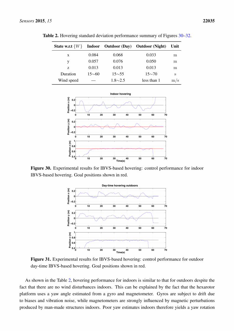
Sensors 2015, 15 22035

Table 2. Hovering standard deviation performance summary of Figures 30–32.

State w.r.t {W} Indoor Outdoor (Day) Outdoor (Night) Unit

x 0.084 0.068 0.033 m

y 0.057 0.076 0.050 m

z 0.013 0.013 0.013 m

Duration 15∼60 15∼55 15∼70 s

Wind speed — 1.8∼2.5 less than 1 m/s

0 10 20 30 40 50 60 70

−0.2

0

0.2

Indoor hovering ground truth from VICON

Posi

tion

x (m

)

0 10 20 30 40 50 60 70

−0.2

0

0.2

Posi

tion

y (m

)

0 10 20 30 40 50 60 700.4

0.6

0.8

1

Posi

tion

z (m

)

Time(s)

0 10 20 30 40 50 60 70

−0.2

0

0.2

Indoor hovering ground truth from VICON

Posi

tion

x (m

)

0 10 20 30 40 50 60 70

−0.2

0

0.2

Posi

tion

y (m

)

0 10 20 30 40 50 60 700.4

0.6

0.8

1

Posi

tion

z (m

)

Time(s)

Figure 30. Experimental results for IBVS-based hovering: control performance for indoorIBVS-based hovering. Goal positions shown in red.

Day-time hovering outdoors

0 10 20 30 40 50 60 70

−0.2

0

0.2

Daytime oudoor hovering ground truth from total station

Posi

tion

x (m

)

0 10 20 30 40 50 60 70

−0.2

0

0.2

Posi

tion

y (m

)

0 10 20 30 40 50 60 700.4

0.6

0.8

1

Posi

tion

z (m

)

Time(s)

Figure 31. Experimental results for IBVS-based hovering: control performance for outdoorday-time IBVS-based hovering. Goal positions shown in red.

As shown in the Table 2, hovering performance for indoors is similar to that for outdoors despite thefact that there are no wind disturbances indoors. This can be explained by the fact that the hexarotorplatform uses a yaw angle estimated from a gyro and magnetometer. Gyros are subject to drift dueto biases and vibration noise, while magnetometers are strongly influenced by magnetic perturbationsproduced by man-made structures indoors. Poor yaw estimates indoors therefore yields a yaw rotation

Sensors 2015, 15 22036

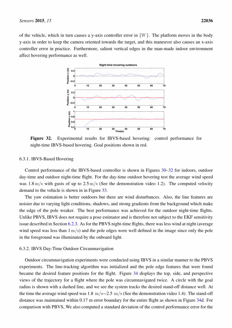
of the vehicle, which in turn causes a y-axis controller error in {W}. The platform moves in the bodyy-axis in order to keep the camera oriented towards the target, and this maneuver also causes an x-axiscontroller error in practice. Furthermore, salient vertical edges in the man-made indoor environmentaffect hovering performance as well.

Night-time hovering outdoors

0 10 20 30 40 50 60 70

−0.2

0

0.2

Night outdoor hovering ground truth from total stationPo

sitio

n x

(m)

0 10 20 30 40 50 60 70

−0.2

0

0.2

Posi

tion

y (m

)

0 10 20 30 40 50 60 700.4

0.6

0.8

1

Posi

tion

z (m

)

Time(s)

Figure 32. Experimental results for IBVS-based hovering: control performance fornight-time IBVS-based hovering. Goal positions shown in red.

6.3.1. IBVS-Based Hovering

Control performance of the IBVS-based controller is shown in Figures 30–32 for indoors, outdoorday-time and outdoor night-time flight. For the day-time outdoor hovering test the average wind speedwas 1.8 m/s with gusts of up to 2.5 m/s (See the demonstration video 1.2). The computed velocitydemand to the vehicle is shown in in Figure 33.

The yaw estimation is better outdoors but there are wind disturbances. Also, the line features arenoisier due to varying light conditions, shadows, and strong gradients from the background which makethe edge of the pole weaker. The best performance was achieved for the outdoor night-time flights.Unlike PBVS, IBVS does not require a pose estimator and is therefore not subject to the EKF sensitivityissue described in Section 6.2.3. As for the PBVS night-time flights, there was less wind at night (averagewind speed was less than 1 m/s) and the pole edges were well defined in the image since only the polein the foreground was illuminated by the onboard light.

6.3.2. IBVS Day-Time Outdoor Circumnavigation

Outdoor circumnavigation experiments were conducted using IBVS in a similar manner to the PBVSexperiments. The line-tracking algorithm was initialized and the pole edge features that were foundbecame the desired feature positions for the flight. Figure 34 displays the top, side, and perspectiveviews of the trajectory for a flight where the pole was circumnavigated twice. A circle with the goalradius is shown with a dashed line, and we see the system tracks the desired stand-off distance well. Atthe time the average wind speed was 1.8 m/s∼2.5 m/s (See the demonstration video 1.4). The stand-offdistance was maintained within 0.17 m error boundary for the entire flight as shown in Figure 34d. Forcomparison with PBVS, We also computed a standard deviation of the control performance error for the

Sensors 2015, 15 22037

same length of flight time (0–75 s) and obtained 0.034 m. IBVS and PBVS show similar performanceas shown in Table 3. The height change near (x = −0.6, y = −0.5) is due to the box that was placedon the ground as a takeoff and landing platform. Since the aircraft maintains a fixed height above theground beneath it, it climbs when flying over the box.

0 10 20 30 40 50 60 70−0.2

−0.15

−0.1

−0.05

0

0.05

0.1

0.15

0.2v∗x and ground truth vx

Time(s)

Velo

city

(m/s

)

Viconv∗x

0 10 20 30 40 50 60 70−0.2

−0.15

−0.1

−0.05

0

0.05

0.1

0.15

0.2v∗y and ground truth vy

Time(s)

Velo

city

(m/s

)

Viconv∗y

0 10 20 30 40 50 60 700

0.2

0.4

0.6

0.8

1Normalized feature RMS error

Time(s)

Feat

ure

erro

r

0 10 20 30 40 50 60 70−0.2

−0.15

−0.1

−0.05

0

0.05

0.1

0.15

0.2v∗x and ground truth vx

Time(s)

Velo

city

(m/s

)

Leika vxv∗x

0 10 20 30 40 50 60 70−0.2

−0.15

−0.1

−0.05

0

0.05

0.1

0.15

0.2v∗y and ground truth vy

Time(s)

Velo

city

(m/s

)

Leika vyv∗y

0 10 20 30 40 50 60 700

0.2

0.4

0.6

0.8

1Normalized feature RMS error

Time(s)

Feat

ure

erro

r

0 10 20 30 40 50 60 70−0.2

−0.15

−0.1

−0.05

0

0.05

0.1

0.15

0.2v∗x and ground truth vx

Time(s)

Velo

city

(m/s

)

Leika vxv∗x

0 10 20 30 40 50 60 70−0.2

−0.15

−0.1

−0.05

0

0.05

0.1

0.15

0.2v∗y and ground truth vy

Time(s)

Velo

city

(m/s

)

Leika vyv∗y

0 10 20 30 40 50 60 700

0.2

0.4

0.6

0.8

1Normalized feature RMS error

Time(s)

Feat

ure

erro

r

Figure 33. Experimental results for IBVS-based hovering: control demand. v∗x (left column)and v∗y (middle column) compared to ground truth. The first row is for indoor hovering whilethe second and the third rows are for day and night-time outdoor hovering. Normalized rootmean squared (RMS) image feature errors for each are shown in the (right column).

6.4. Manually Piloted Experiments

The aim of these experiments was to determine how well a human pilot could perform the inspectiontasks, hovering and circumnavigation, that we have demonstrated autonomously. Manual pilotingrequires great skill and people with this skill are quite scarce. The key skill is hand eye coordination,adjusting the vehicle’s position by controlling roll and pitch angle joysticks. These joysticks effectivelycontrol vehicle acceleration which is more difficult for humans to master than the more common rate,or velocity, control inputs. The controls are effected with respect to the vehicle’s coordinate frame, and

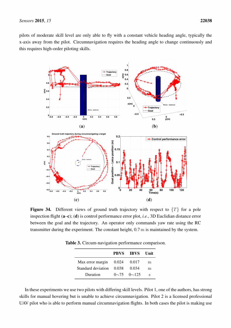
Sensors 2015, 15 22038

pilots of moderate skill level are only able to fly with a constant vehicle heading angle, typically thex-axis away from the pilot. Circumnavigation requires the heading angle to change continuously andthis requires high-order piloting skills.

−0.8 −0.6 −0.4 −0.2 0 0.2 0.4 0.6 0.80

0.2

0.4

0.6

0.8

1

x(m)

Ground truth trajectory during circumnavigating a target

z(m

)

TrajectoryGoal

Pole centre

(a)

−0.5

0

0.5

−0.50

0.5

0

0.2

0.4

0.6

0.8

1

y(m)

Ground truth trajectory during circumnavigating a target

x(m)

z(m

)

TrajectoryGoal

Pole centre

(b)

−0.8 −0.6 −0.4 −0.2 0 0.2 0.4 0.6 0.8−0.8

−0.6

−0.4

−0.2

0

0.2

0.4

0.6

0.8

x(m)

Ground truth trajectory during circumnavigating a target

y(m

)

TrajectoryGoal

Pole centre

(c)

0 20 40 60 80 100 1200

0.05

0.1

0.15

0.2

Time(s)

Goa

l pos

ition

− L

eica

pos

ition

(m)

Control performance error

(d)

Figure 34. Different views of ground truth trajectory with respect to {T} for a poleinspection flight (a–c); (d) is control performance error plot, i.e., 3D Euclidian distance errorbetween the goal and the trajectory. An operator only commands yaw rate using the RCtransmitter during the experiment. The constant height, 0.7 m is maintained by the system.

Table 3. Circum-navigation performance comparison.

PBVS IBVS Unit

Max error margin 0.024 0.017 m

Standard deviation 0.038 0.034 m

Duration 0∼75 0∼125 s

In these experiments we use two pilots with differing skill levels. Pilot 1, one of the authors, has strongskills for manual hovering but is unable to achieve circumnavigation. Pilot 2 is a licensed professionalUAV pilot who is able to perform manual circumnavigation flights. In both cases the pilot is making use

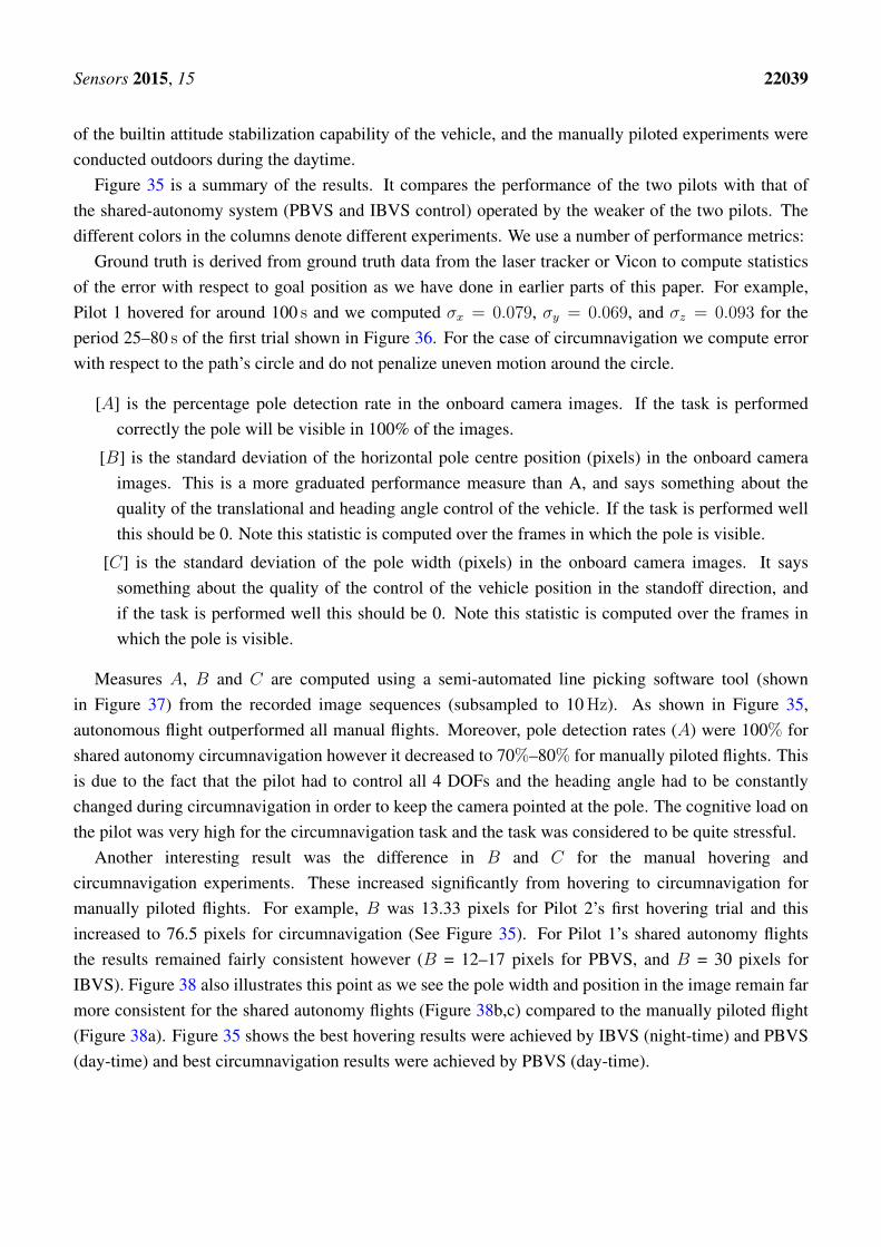
Sensors 2015, 15 22039

of the builtin attitude stabilization capability of the vehicle, and the manually piloted experiments wereconducted outdoors during the daytime.

Figure 35 is a summary of the results. It compares the performance of the two pilots with that ofthe shared-autonomy system (PBVS and IBVS control) operated by the weaker of the two pilots. Thedifferent colors in the columns denote different experiments. We use a number of performance metrics:

Ground truth is derived from ground truth data from the laser tracker or Vicon to compute statisticsof the error with respect to goal position as we have done in earlier parts of this paper. For example,Pilot 1 hovered for around 100 s and we computed σx = 0.079, σy = 0.069, and σz = 0.093 for theperiod 25–80 s of the first trial shown in Figure 36. For the case of circumnavigation we compute errorwith respect to the path’s circle and do not penalize uneven motion around the circle.

[A] is the percentage pole detection rate in the onboard camera images. If the task is performedcorrectly the pole will be visible in 100% of the images.

[B] is the standard deviation of the horizontal pole centre position (pixels) in the onboard cameraimages. This is a more graduated performance measure than A, and says something about thequality of the translational and heading angle control of the vehicle. If the task is performed wellthis should be 0. Note this statistic is computed over the frames in which the pole is visible.

[C] is the standard deviation of the pole width (pixels) in the onboard camera images. It sayssomething about the quality of the control of the vehicle position in the standoff direction, andif the task is performed well this should be 0. Note this statistic is computed over the frames inwhich the pole is visible.

Measures A, B and C are computed using a semi-automated line picking software tool (shownin Figure 37) from the recorded image sequences (subsampled to 10 Hz). As shown in Figure 35,autonomous flight outperformed all manual flights. Moreover, pole detection rates (A) were 100% forshared autonomy circumnavigation however it decreased to 70%–80% for manually piloted flights. Thisis due to the fact that the pilot had to control all 4 DOFs and the heading angle had to be constantlychanged during circumnavigation in order to keep the camera pointed at the pole. The cognitive load onthe pilot was very high for the circumnavigation task and the task was considered to be quite stressful.

Another interesting result was the difference in B and C for the manual hovering andcircumnavigation experiments. These increased significantly from hovering to circumnavigation formanually piloted flights. For example, B was 13.33 pixels for Pilot 2’s first hovering trial and thisincreased to 76.5 pixels for circumnavigation (See Figure 35). For Pilot 1’s shared autonomy flightsthe results remained fairly consistent however (B = 12–17 pixels for PBVS, and B = 30 pixels forIBVS). Figure 38 also illustrates this point as we see the pole width and position in the image remain farmore consistent for the shared autonomy flights (Figure 38b,c) compared to the manually piloted flight(Figure 38a). Figure 35 shows the best hovering results were achieved by IBVS (night-time) and PBVS(day-time) and best circumnavigation results were achieved by PBVS (day-time).

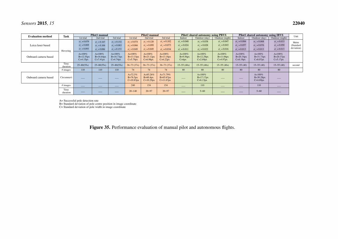
Sensors 2015, 15 22040

1st trial 2nd trial 3rd trial 1st trial 2nd trial 3rd trial Indoor Outdoor (day) Outdoor (night) Indoor Outdoor (day) Outdoor (night)

Leica laser basedMetre

(Standard deviation)

Onboard camera basedA=100%B=12.55pxC=4.15px

A=100%B=16.64pxC=7.41px

A=100%B=16.73pxC=4.74px

A=100%B=13.33pxC=5.79px

A=100%B=23.12pxC=6.98px

A=100%B=13.18pxC=6.22px

A=100%B=9.56pxC=6px

A=100%B=12.29pxC=2.69px

A=100%B=11.06pxC=4.97px

A=100%B=20.34pxC=8.19px

A=100%B=31.73pxC=8.07px

A=100%B=20.37pxC=5.17px

Time duration 25~80(55s) 25~80(55s) 25~80(55s) 36~73 (37s) 36~73 (37s) 36~73 (37s) 15~55 (40s) 15~55 (40s) 15~55 (40s) 15~55 (40) 15~55 (40) 15~55 (40) second

# images 110 110 110 74 74 74 80 80 80 80 80 80

Onboard camera based Circumnavi ___ ___ ___A=72.5%B=76.5pxC=10.83px

A=85.26%B=60.4pxC=10.29px

A=71.79%B=65.67pxC=11.67px

___A=100%B=17.17pxC=6.13px

___ ___A=100%B=30.28pxC=4.69px

___

# images ___ ___ ___ 240 154 154 ___ 110 ___ ___ 110 ___

Time duration ___ ___ ___ 20~140 20~97 20~97 ___ 5~60 ___ ___ 5~60 ___

A= Successful pole detection rateB= Standard deviation of pole centre position in image coordinateC= Standard deviation of pole width in image coordinate

Hovering

Evaluation method UnitPilot1 manual Pilot2 manual Pilot1 shared autonomy using PBVS Pilot1 shared autonomy using IBVSTaskσ x = 0.079σ y = 0.069σ z = 0.093

σ x = 0.167σ y = 0.106σ z = 0.086

σ x = 0.152σ y = 0.083σ z = 0.153

σ x = 0.120σ y = 0.099σ z = 0.049

σ x = 0.102σ y = 0.073σ z = 0.034

σ x = 0.048σ y = 0.024σ z = 0.011

σ x = 0.038σ y = 0.028σ z = 0.022

σ x = 0.047σ y = 0.043σ z = 0.016

σ x = 0.084σ y = 0.057σ z = 0.013

σ x = 0.068σ y = 0.076σ z = 0.013

σ x = 0.033σ y = 0.050σ z = 0.013

σ x = 0.074σ y = 0.066σ z = 0.049

Figure 35. Performance evaluation of manual pilot and autonomous flights.

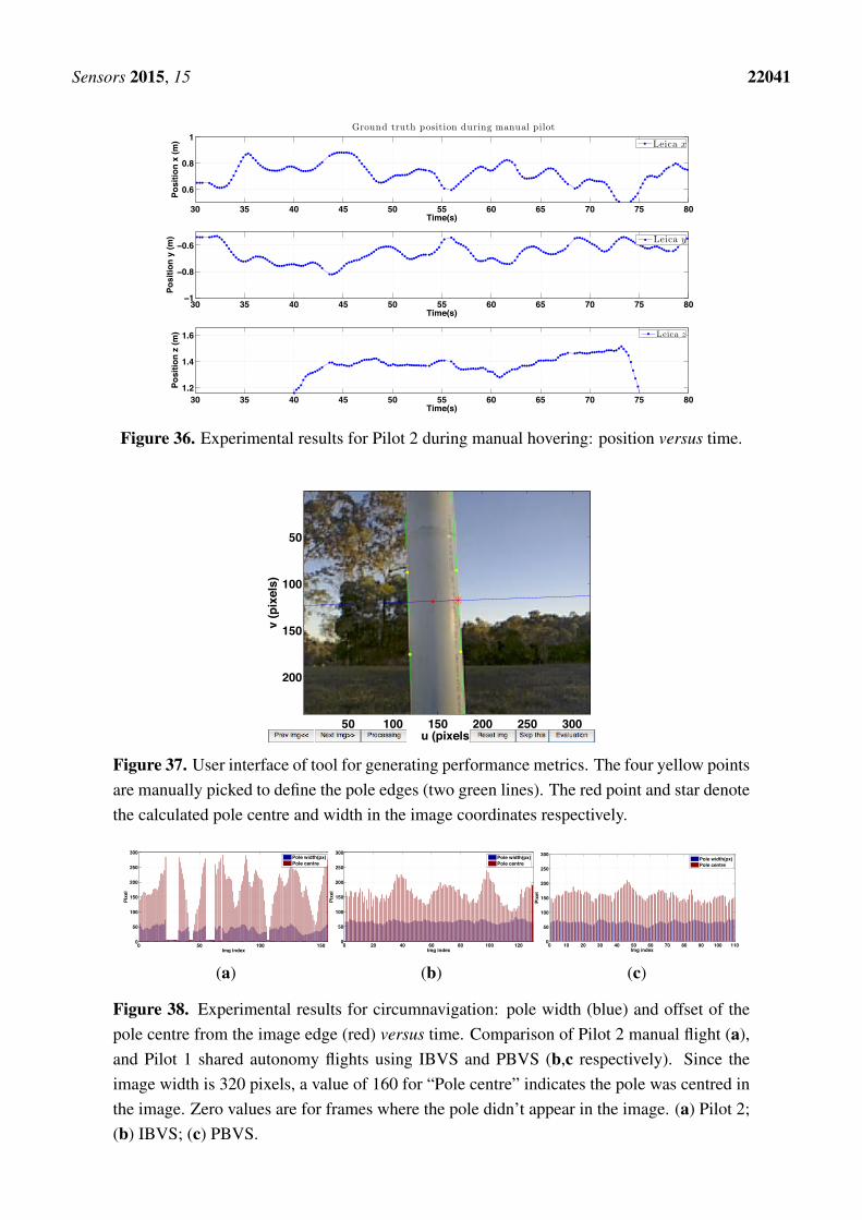
Sensors 2015, 15 22041

30 35 40 45 50 55 60 65 70 75 80

0.6

0.8

1Ground truth position during manual pilot

Time(s)

Posi

tion

x (m

)

Leica x

30 35 40 45 50 55 60 65 70 75 80−1

−0.8

−0.6

Time(s)

Posi

tion

y (m

)

Leica y

30 35 40 45 50 55 60 65 70 75 801.2

1.4

1.6

Time(s)

Posi

tion

z (m

)

Leica z

Figure 36. Experimental results for Pilot 2 during manual hovering: position versus time.

u (pixels)

v (p

ixel

s)

RGB image

50 100 150 200 250 300

50

100

150

200

Figure 37. User interface of tool for generating performance metrics. The four yellow pointsare manually picked to define the pole edges (two green lines). The red point and star denotethe calculated pole centre and width in the image coordinates respectively.

0 50 100 1500

50

100

150

200

250

300

Img index

Pixe

l

Pole width(px)Pole centre

(a)

0 20 40 60 80 100 1200

50

100

150

200

250

300

Img index

Pixe

l

Pole width(px)Pole centre

(b)

0 10 20 30 40 50 60 70 80 90 100 1100

50

100

150

200

250

300

Img index

Pixe

l

Pole width(px)Pole centre

(c)

Figure 38. Experimental results for circumnavigation: pole width (blue) and offset of thepole centre from the image edge (red) versus time. Comparison of Pilot 2 manual flight (a),and Pilot 1 shared autonomy flights using IBVS and PBVS (b,c respectively). Since theimage width is 320 pixels, a value of 160 for “Pole centre” indicates the pole was centred inthe image. Zero values are for frames where the pole didn’t appear in the image. (a) Pilot 2;(b) IBVS; (c) PBVS.

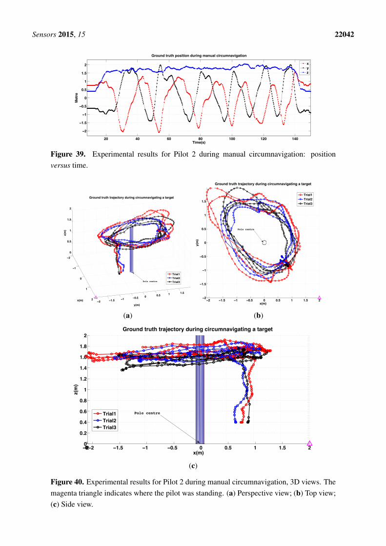
Sensors 2015, 15 22042

20 40 60 80 100 120 140

−2

−1.5

−1

−0.5

0

0.5

1

1.5

2

Ground truth position during manual circumnavigation

Time(s)

Met

re

xyz

Figure 39. Experimental results for Pilot 2 during manual circumnavigation: positionversus time.

−2

−1

0

1

2−2 −1.5 −1 −0.5 0 0.5 1 1.5

0

0.5

1

1.5

2

y(m)

Ground truth trajectory during circumnavigating a target

x(m)

z(m

)

Trial1Trial2Trial3Pole centre

(a)

−2 −1.5 −1 −0.5 0 0.5 1 1.5 2−2

−1.5

−1

−0.5

0

0.5

1

1.5

x(m)

Ground truth trajectory during circumnavigating a target

y(m

)Trial1Trial2Trial3

Pole centre

(b)

−2 −1.5 −1 −0.5 0 0.5 1 1.5 2−2−1010

0.2

0.4

0.6

0.8

1

1.2

1.4

1.6

1.8

2

x(m)

Ground truth trajectory during circumnavigating a target

z(m

)

Trial1Trial2Trial3

Pole centre

(c)

Figure 40. Experimental results for Pilot 2 during manual circumnavigation, 3D views. Themagenta triangle indicates where the pilot was standing. (a) Perspective view; (b) Top view;(c) Side view.

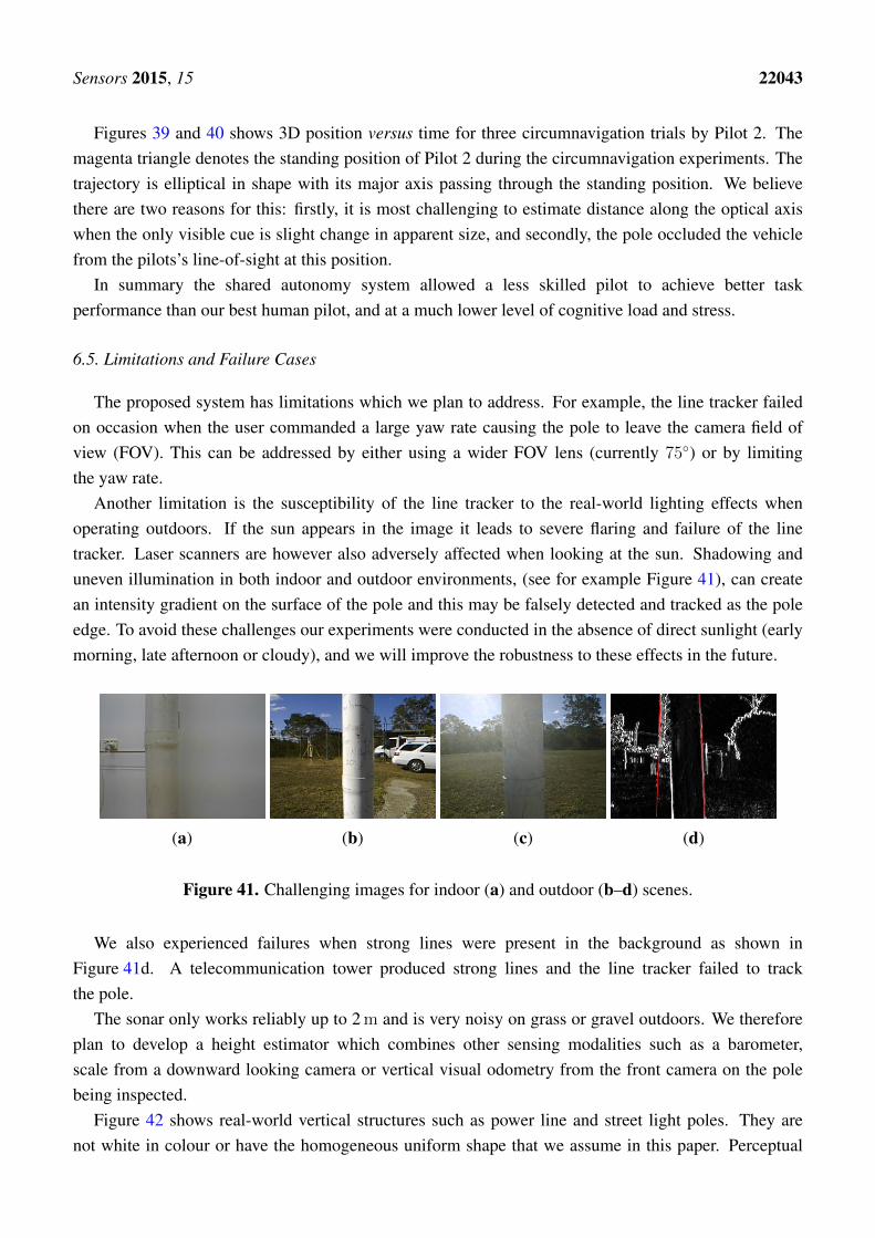
Sensors 2015, 15 22043

Figures 39 and 40 shows 3D position versus time for three circumnavigation trials by Pilot 2. Themagenta triangle denotes the standing position of Pilot 2 during the circumnavigation experiments. Thetrajectory is elliptical in shape with its major axis passing through the standing position. We believethere are two reasons for this: firstly, it is most challenging to estimate distance along the optical axiswhen the only visible cue is slight change in apparent size, and secondly, the pole occluded the vehiclefrom the pilots’s line-of-sight at this position.

In summary the shared autonomy system allowed a less skilled pilot to achieve better taskperformance than our best human pilot, and at a much lower level of cognitive load and stress.

6.5. Limitations and Failure Cases

The proposed system has limitations which we plan to address. For example, the line tracker failedon occasion when the user commanded a large yaw rate causing the pole to leave the camera field ofview (FOV). This can be addressed by either using a wider FOV lens (currently 75◦) or by limitingthe yaw rate.

Another limitation is the susceptibility of the line tracker to the real-world lighting effects whenoperating outdoors. If the sun appears in the image it leads to severe flaring and failure of the linetracker. Laser scanners are however also adversely affected when looking at the sun. Shadowing anduneven illumination in both indoor and outdoor environments, (see for example Figure 41), can createan intensity gradient on the surface of the pole and this may be falsely detected and tracked as the poleedge. To avoid these challenges our experiments were conducted in the absence of direct sunlight (earlymorning, late afternoon or cloudy), and we will improve the robustness to these effects in the future.

(a) (b) (c) (d)

Figure 41. Challenging images for indoor (a) and outdoor (b–d) scenes.

We also experienced failures when strong lines were present in the background as shown inFigure 41d. A telecommunication tower produced strong lines and the line tracker failed to trackthe pole.

The sonar only works reliably up to 2 m and is very noisy on grass or gravel outdoors. We thereforeplan to develop a height estimator which combines other sensing modalities such as a barometer,scale from a downward looking camera or vertical visual odometry from the front camera on the polebeing inspected.

Figure 42 shows real-world vertical structures such as power line and street light poles. They arenot white in colour or have the homogeneous uniform shape that we assume in this paper. Perceptual

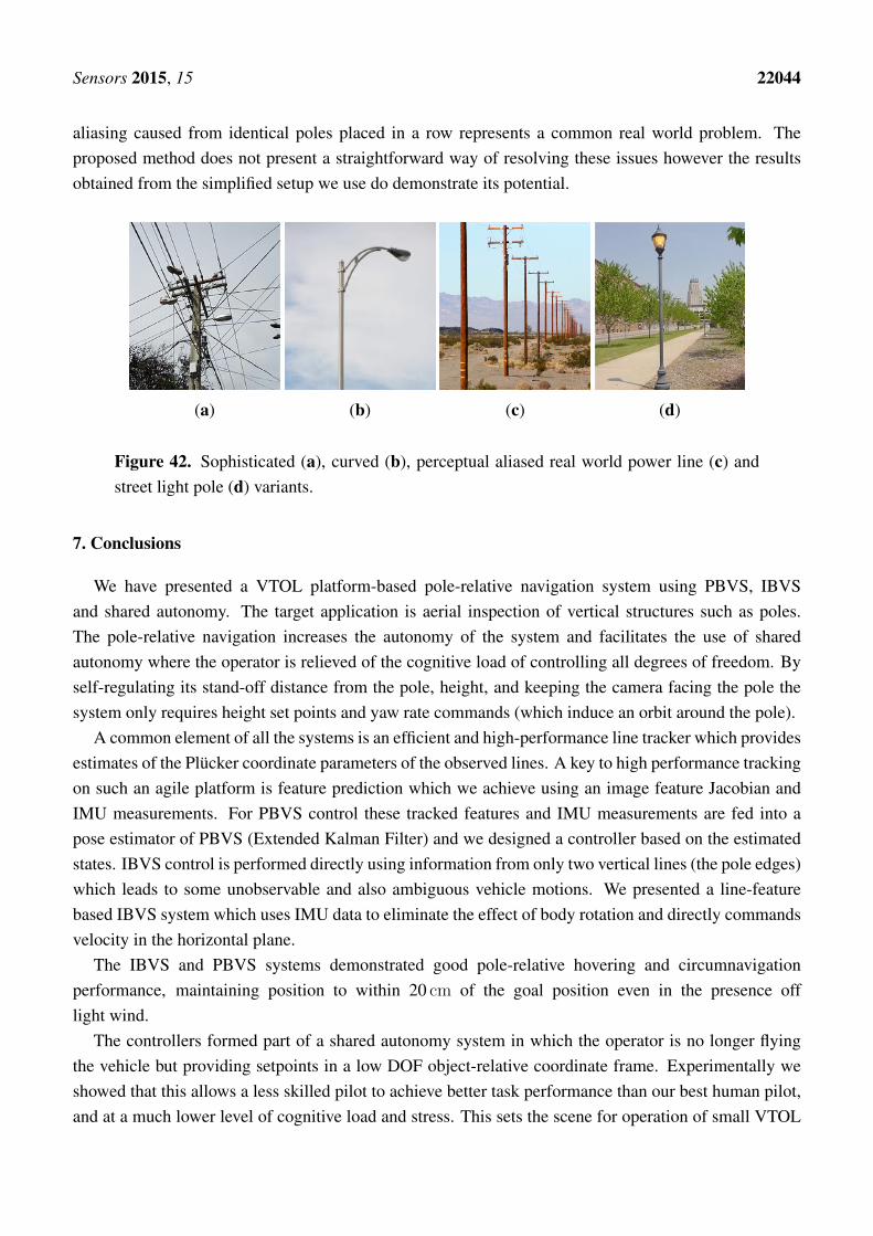
Sensors 2015, 15 22044

aliasing caused from identical poles placed in a row represents a common real world problem. Theproposed method does not present a straightforward way of resolving these issues however the resultsobtained from the simplified setup we use do demonstrate its potential.

(a) (b) (c) (d)

Figure 42. Sophisticated (a), curved (b), perceptual aliased real world power line (c) andstreet light pole (d) variants.

7. Conclusions

We have presented a VTOL platform-based pole-relative navigation system using PBVS, IBVSand shared autonomy. The target application is aerial inspection of vertical structures such as poles.The pole-relative navigation increases the autonomy of the system and facilitates the use of sharedautonomy where the operator is relieved of the cognitive load of controlling all degrees of freedom. Byself-regulating its stand-off distance from the pole, height, and keeping the camera facing the pole thesystem only requires height set points and yaw rate commands (which induce an orbit around the pole).

A common element of all the systems is an efficient and high-performance line tracker which providesestimates of the Plücker coordinate parameters of the observed lines. A key to high performance trackingon such an agile platform is feature prediction which we achieve using an image feature Jacobian andIMU measurements. For PBVS control these tracked features and IMU measurements are fed into apose estimator of PBVS (Extended Kalman Filter) and we designed a controller based on the estimatedstates. IBVS control is performed directly using information from only two vertical lines (the pole edges)which leads to some unobservable and also ambiguous vehicle motions. We presented a line-featurebased IBVS system which uses IMU data to eliminate the effect of body rotation and directly commandsvelocity in the horizontal plane.

The IBVS and PBVS systems demonstrated good pole-relative hovering and circumnavigationperformance, maintaining position to within 20 cm of the goal position even in the presence offlight wind.

The controllers formed part of a shared autonomy system in which the operator is no longer flyingthe vehicle but providing setpoints in a low DOF object-relative coordinate frame. Experimentally weshowed that this allows a less skilled pilot to achieve better task performance than our best human pilot,and at a much lower level of cognitive load and stress. This sets the scene for operation of small VTOL

Sensors 2015, 15 22045

platforms to perform cost-effective single person inspection jobs, rather than the three person crews thatare currently the norm.

Finally, even though both systems demonstrate good performance, we prefer IBVS over PBVS fortwo reasons. Firstly, PBVS requires a pose estimator which takes image features as input and computesthe metric pose of a camera. Development of a robust vision-based pose estimator that can be usedin varying environments is difficult. Secondly, IBVS is relatively easy to implement since it omits thepose estimation step, and utilize the image features directly. Although IBVS can degrade observabilityand be poorly conditioned due to a linearization of a highly non-linear model, it works on our poletracking application.

Acknowledgments

The authors would like to thank Aaron Mcfadyen for assistance while using the VICON system,Navinda Kottege for providing the Leica ROS software and Kyran Findlater for supplying the LED light.In addition we thank to Peter Reid for manual pilot experiments.

Author Contributions

Inkyu Sa contributed to the development of the systems including implementation, field tests, andthe manuscript writing. Stefan Hrabar contributed to the manuscript writing, providing significantsuggestions on the development, and supporting field tests. Peter Corke provided the manuscript writingand guided the whole study.

Conflicts of Interest

The authors declare no conflict of interest.

References

1. Echelon. Monitored Outdoor Lighting. Available online: http://info.echelon.com/Whitepaper-Monitored-Outdoor-Lighting.html (accessed on 27 August 2015).

2. Pratt, K.S.; Murphy, R.R.; Stover, S.; Griffin, C. CONOPS and autonomy recommendations forVTOL small unmanned aerial system based on Hurricane Katrina operations. J. Field Robot. 2009,26, 636–650.

3. Consumer Reports Magazine. Available online: http://www.consumerreports.org/cro/magazine-archive/may-2009/may-2009-toc.htm (accessed on 27 August 2015).

4. Balaguer, C.; Gimenez, A.; Jardon, A. Climbing Robots’ Mobility for Inspection and Maintenanceof 3D Complex Environments. Auton. Robot. 2005, 18, 157–169.

5. Kim, S.; Spenko, M.; Trujillo, S.; Heyneman, B.; Santos, D.; Cutkosky, M. Smooth VerticalSurface Climbing With Directional Adhesion. IEEE Trans. Robot. 2008, 24, 65–74.

6. Xu, F.; Wang, X.; Wang, L. Cable inspection robot for cable-stayed bridges: Design, analysis, andapplication. J. Field Robot. 2011, 28, 441–459.

Sensors 2015, 15 22046

7. Haynes, G.C.; Khripin, A.; Lynch, G.; Amory, J.; Saunders, A.; Rizzi, A.A.; Koditschek, D.E.Rapid Pole Climbing with a Quadrupedal Robot. In Proceedings of the IEEE InternationalConference on Robotics and Automation, Kobe, Japan, 12–17 May 2009; pp. 2767–2772.

8. Parness, A.; Frost, M.; King, J.; Thatte, N. Demonstrations of gravity-independent mobility anddrilling on natural rock using microspines. In Proceedings of the IEEE International Conferenceon Robotics and Automation, Saint Paul, MN, USA, 14–18 May 2012; pp. 3547–3548.

9. Ahmadabadi, M.; Moradi, H.; Sadeghi, A.; Madani, A.; Farahnak, M. The evolution of UT poleclimbing robots. In Proceedings of the 2010 1st International Conference on Applied Robotics forthe Power Industry (CARPI), Montreal, QC, Canada, 5–7 October 2010; pp. 1–6.

10. Kendoul, F. Survey of advances in guidance, navigation, and control of unmanned rotorcraftsystems. J. Field Robot. 2012, 29, 315–378.

11. Voigt, R.; Nikolic, J.; Hurzeler, C.; Weiss, S.; Kneip, L.; Siegwart, R. Robust embedded egomotionestimation. In Proceedings of the IEEE International Conference on Intelligent Robots andSystems, San Francisco, CA, USA, 25–30 September 2011; pp. 2694–2699.

12. Burri, M.; Nikolic, J.; Hurzeler, C.; Caprari, G.; Siegwart, R. Aerial service robots for visualinspection of thermal power plant boiler systems. In Proceedings of the International Conference onApplied Robotics for the Power Industry, Zurich, Switzerland, 11–13 September 2012; pp. 70–75.

13. Nikolic, J.; Burri, M.; Rehder, J.; Leutenegger, S.; Huerzeler, C.; Siegwart, R. A UAV system forinspection of industrial facilities. In Proceedings of the IEEE Aerospace Conference, Big Sky, MT,USA, 2–9 March 2013; pp. 1–8.

14. Ortiz, A.; Bonnin-Pascual, F.; Garcia-Fidalgo, E. Vessel Inspection: A Micro-Aerial Vehicle-basedApproach. J. Intell. Robot. Syst. 2013, 76, 151–167.

15. Eich, M.; Bonnin-Pascual, F.; Garcia-Fidalgo, E.; Ortiz, A.; Bruzzone, G.; Koveos, Y.; Kirchner, F.A Robot Application for Marine Vessel Inspection. J. Field Robot. 2014, 31, 319–341.

16. Bachrach, A.; Prentice, S.; He, R.; Roy, N. RANGE–Robust autonomous navigation in GPS-deniedenvironments. J. Field Robot. 2011, 28, 644–666.

17. Shen, S.; Michael, N.; Kumar, V. Autonomous Multi-Floor Indoor Navigation with aComputationally Constrained MAV. In Proceedings of the IEEE International Conference onRobotics and Automation, Shanghai, China, 9–13 May 2011; pp. 20–25.

18. Sa, I.; Corke, P. Improved line tracking using IMU and Vision for visual servoing. In Proceedingsof the Australasian Conference on Robotics and Automation, University of New South Wales,Sydney, Australia, 2–4 December 2013.

19. Sa, I.; Hrabar, S.; Corke, P. Outdoor Flight Testing of a Pole Inspection UAV IncorporatingHigh-Speed Vision. In Proceedings of the International Conference on Field and Service Robotics,Brisbane, Australia, 9–11 December 2013.

20. Sa, I.; Hrabar, S.; Corke, P. Inspection of Pole-Like Structures Using a Vision-Controlled VTOLUAV and Shared Autonomy. In Proceedings of the IEEE International Conference on IntelligentRobots and Systems, Chicago, IL, USA, 14–18 September 2014; pp. 4819–4826.

21. Sa, I.; Corke, P. Close-quarters Quadrotor flying for a pole inspection with position basedvisual servoing and high-speed vision. In Proceedings of the IEEE International Conference onUnmanned Aircraft Systems, Orlando, FL, USA, 27–30 May 2014; pp. 623–631.

Sensors 2015, 15 22047

22. Video demonstration. Available online: http://youtu.be/ccS85_EDl9A (accessed on 27 August2015).

23. Hough, P. Machine Analysis of Bubble Chamber Pictures. In Proceedings of the InternationalConference on High Energy Accelerators and Instrumentation, Geneva, Switzerland, 14–19September 1959.

24. Shi, D.; Zheng, L.; Liu., J. Advanced Hough Transform Using A Multilayer Fractional FourierMethod. IEEE Trans. Image Process. 2010, doi:10.1109/TIP.2010.2042102.

25. Hager, G.; Toyama, K. X vision: A portable substrate for real-time vision applications.Comput. Vis. Image Understand. 1998, 69, 23–37.

26. Bartoli, A.; Sturm, P. The 3D line motion matrix and alignment of line reconstructions. InProceedings of the IEEE Conference on Computer Vision and Pattern Recognition, Kauai, USA,8–14 December 2001; Volume 1, pp. 1–287.

27. Hartley, R.; Zisserman, A. Multiple View Geometry in Computer Vision; Cambridge UniversityPress: Cambridge, UK, 2003.

28. Bartoli, A.; Sturm, P. Structure-from-motion using lines: Representation, triangulation, and bundleadjustment. Comput. Vis. Image Understand. 2005, 100, 416–441.

29. Mahony, R.; Hamel, T. Image-based visual servo control of aerial robotic systems using linearimage features. IEEE Trans. Robot. 2005, 21, 227–239.

30. Solà, J.; Vidal-Calleja, T.; Civera, J.; Montiel, J.M. Impact of Landmark Parametrization onMonocular EKF-SLAM with Points and Lines. Int. J. Comput. Vis. 2012, 97, 339–368.

31. Chaumette, F.; Hutchinson, S. Visual servo control. I. Basic approaches. IEEE Robot. Autom.Mag. 2006, 13, 82–90.

32. Fischler, M.; Bolles, R. Random sample consensus: A paradigm for model fitting with applicationsto image analysis and automated cartography. Commun. ACM, 1981, 24, 381–395.

33. Durrant-Whyte, H. Introduction to Estimation and the Kalman Filter; Technical Report; TheUniversity of Sydney: Sydney, Australia, 2001.

34. Mahony, R.; Kumar, V.; Corke, P. Modeling, Estimation and Control of Quadrotor Aerial Vehicles.IEEE Robot. Autom. Mag. 2012, doi:10.1109/MRA.2012.2206474.

35. Leishman, R.; Macdonald, J.; Beard, R.; McLain, T. Quadrotors and Accelerometers: StateEstimation with an Improved Dynamic Model. IEEE Control Syst. 2014, 34, 28–41.

36. Corke, P. Robotics, Vision & Control: Fundamental Algorithms in MATLAB; Springer: Brisbane,Australia, 2011. ISBN 978-3-642-20143-1.

37. Corke, P.; Hutchinson, S. A new partitioned approach to image-based visual servo control.IEEE Trans. Robot. Autom. 2001, 17, 507–515.

38. Malis, E.; Rives, P. Robustness of image-based visual servoing with respect to depth distributionerrors. In Proceedings of the IEEE International Conference on Robotics and Automation, Taipei,Taiwan, 14–19 September 2003; pp. 1056–1061.

39. Espiau, B.; Chaumette, F.; Rives, P. A new approach to visual servoing in robotics. IEEE Trans.Robot. Autom. 1992, 8, 313–326.

Sensors 2015, 15 22048

40. Pissard-Gibollet, R.; Rives, P. Applying visual servoing techniques to control a mobile hand-eyesystem. In Proceedings of the IEEE International Conference on Robotics and Automation,Nagoya, Japan, 21–27 May 1995; pp. 166–171.

41. Briod, A.; Zufferey, J.C.; Floreano, D. Automatically calibrating the viewing direction of optic-flowsensors. In Proceedings of the IEEE International Conference on Robotics and Automation, St Paul,MN, USA, 14–18 May 2012; pp. 3956–3961.

42. Corke, P.; Hutchinson, S. Real-time vision, tracking and control. In Proceedings of the IEEEInternational Conference on Robotics and Automation, Saint Paul, MN, USA, 14–18 May 2012;pp. 622–629.

43. Feddema, J.; Mitchell, O.R. Vision-guided servoing with feature-based trajectory generation [forrobots]. IEEE Trans. Robot. Autom. 1989, 5, 691–700.

44. Hosoda, K.; Asada, M. Versatile visual servoing without knowledge of true Jacobian. InProceedings of the IEEE International Conference on Intelligent Robot Systems, Munich, Germany,12–16 September 1994; pp. 186–193.

45. Omari, S.; Ducard, G. Metric Visual-Inertial Navigation System Using Single Optical FlowFeature. In Proceedings of the European Contol Conference, Zurich, Switzerland, 17–19 July 2013.

46. Quigley, M.; Conley, K.; Gerkey, B.; Faust, J.; Foote, T.B.; Leibs, J.; Wheeler, R.; Ng, A.Y. ROS:An open-source Robot Operating System. In Proceedings of the IEEE International Conference onRobotics and Automation Workshop on Open Source Software, Kobe, Japan, 12–17 May 2009;pp. 5–11.

47. O’Sullivan, L.; Corke, P. Empirical Modelling of Rolling Shutter Effect. In Proceedingsof the IEEE International Conference on Robotics and Automation, Hong Kong, China,31 May–7 June 2014.

48. Achtelik, M.; Achtelik, M.; Weiss, S.; Siegwar, R. Onboard IMU and Monocular Vision BasedControl for MAVs in Unknown In- and Outdoor Environments. In Proceedings of the IEEEInternational Conference on Robotics and Automation, Shanghai, China, 9–13 May 2011.

49. Leica TS30. Available online: http://www.leica-geosystems.com/en/Engineering-Monitoring-TPS-Leica-TS30_77093.htm (accessed on 27 August 2015).

50. Bachrach, A.G. Autonomous Flight in Unstructured and Unknown Indoor Environments. Master’sThesis, MIT, Cambridge, MA, USA, 2009.

51. Abbeel, P.; Coates, A.; Montemerlo, M.; Ng, A.Y.; Thrun, S. Discriminative Training of KalmanFilters. In Proceedings of the Robotics: Science and Systems, Cambridge, MA, USA, 8–11 June2005; pp. 289–296.

© 2015 by the authors; licensee MDPI, Basel, Switzerland. This article is an open access articledistributed under the terms and conditions of the Creative Commons Attribution license(http://creativecommons.org/licenses/by/4.0/).