sensor-based 3-d pose estimation and control of rotary...

Sensor-based 3-D Pose Estimation and Controlof Rotary-wing UAVs using a 2-D LiDAR

Alexandre Gomes1, Bruno J. Guerreiro1?, Rita Cunha1, Carlos Silvestre2,1??,and Paulo Oliveira3,1

1 Institute for Systems and Robotics (ISR/IST), LARSYS,Instituto Superior Tecnico, Universidade de Lisboa, Portugal

2 Department of Electrical and Computer Engineering,Faculty of Science and Technology, University of Macau, Taipa, Macau SAR, China

3 Associated Laboratory for Energy, Transports, and Aeronautics (LAETA),Instituto Superior Tecnico, Universidade de Lisboa, Portugal

Abstract. This paper addresses the problem of deriving attitude es-timation and trajectory tracking strategies for unmanned aerial vehi-cles (UAVs) using exclusively on-board sensors. The perception of thevehicle position and attitude relative to a structure is achieved by ro-bustly comparing a known pier geometry or map with the data providedby a LiDAR sensor, solving an optimization problem and also robustlyidentifying outliers. Building on this information, several methods arediscussed for obtaining the attitude of the vehicle with respect to thestructure, including a nonlinear observer to estimate the vehicle attitudeon SO(3). A simple nonlinear control strategy is also designed with theobjective of providing an accurate trajectory tracking control relative tothe structure, and experimental results are provided for the performanceevaluation of the proposed algorithms.

1 Introduction

Unmanned aerial vehicles (UAVs), more informally known as drones, were ini-tially developed within a military context [3, 16], yet soon the world realizedthat these small vehicles could be used in tasks other than warfare, such as theinspection of infrastructures. The technological evolution has led to an increasein the demand for more and larger wind turbines, cellphone towers, and powerlines, to name a few. All these large buildings and facilities are critical infras-tructures that require maintenance through structural inspections and healthmonitoring, which can become inefficient in situations where the access is dif-ficult, time-consuming, and often dangerous. Small vehicles such as UAVs con-stitute a tailor-made solution, able to navigate and track trajectories with greataccuracy. While the motion control of aerial vehicles in free flight is reaching

? Corresponding Author. E-mail: [email protected].?? C. Silvestre is also on leave from the Department of Electrical and Computer Engi-

neering, Instituto Superior Tecnico, Universidade de Lisboa, Portugal.

2 Alexandre Gomes et al.

its maturity, new challenges that involve interaction with the environment arebeing embraced. Using local sensors, such as inertial measurement units (IMUs)and light detection and ranging (LiDAR) sensors, some quantities required forcontrol tasks can be obtained depending solely on the vehicle. Having a GPSenables these vehicles to fly autonomously, a feature that can become compro-mised in the vicinity of large infrastructures, as the GPS signal can be easilyoccluded by these structures. This paper aims to take the interaction with theenvironment one step further, using information from the vehicle’s surroundings.

Using LiDARs for self localization in GPS-denied environments is by now anubiquitous and mandatory technology in mobile robots [15], and more applica-tions of this type of sensor are emerging for UAVs, as in [8] or [6]. In comparisonwith video cameras, also used in visual structure from motion algorithms [17],LiDARs offer better depth resolution, range, and horizontal field of view at thecost of lower horizontal and vertical resolution. Building on the work presentedin [7, 4], this work extends the relative pose of the vehicle to include its attitude,allowing a full 3-D structure dependent trajectory to be defined, provided that aknown geometry in the environment is present (such as a pier). For detecting thegeometric primitives necessary for relative pose estimation, several approachesare available, either for circular-like piers [14] or for planar-wise structures [11],where the edges detected in the environment are the foundations to obtain the 3-D attitude estimate. Given the resolution limitations of the considered LiDARs,this work assumes the existence of a rectangular section pier, for which one ortwo faces are always visible to the LiDAR. An edge detection strategy is pro-posed, and based on simple geometric properties, the variations of the detectededges can be used to extract a pair of 3-D vectors, in the vehicle and worldframes. With these vector pairs, several attitude estimation algorithms can beused, such as the solution to the well-known Wahba’s problem [10], or moreevolved nonlinear filters [1]. This paper also proposes a nonlinear filter to com-pute the rotation matrix describing the motion of a vehicle based on the fusionof LiDAR and IMU measurements. Finally, the motion control design yields atrajectory tracking controller solely based on local sensory information, thereforeproviding a relative positioning solution for GPS-denied environments.

The paper is organized as follows. Section 2 discusses the edge detectionapproach, combining algorithms such as the Split & Merge and least square fit-ting. Section 3 designs several methods to obtain the vehicle’s attitude from thedetected edges. Next, Section 4 discusses the control strategies developed for tra-jectory tracking, whereas Section 5 compares the attitude estimation algorithmsusing experimental data and validates the control strategy with experimentaltrials. Finally, some concluding remarks are offered in Section 6.

2 Environment Perception

Detecting a structure and obtaining the necessary information to determine thevehicle’s attitude greatly depends on the knowledge of its geometry. This paperconsiders piers with a rectangular section, where the LiDAR can see one or two

Sensor-based Estimation and Control using a 2-D LiDAR 3

py [m]

-0.1 -0.05 0 0.05 0.1 0.15 0.2

px [m

]

0.75

0.8

0.85

0.9

0.95

1

Data PointsRectangle's EdgesRectangle's Center

py [m]

-0.15 -0.1 -0.05 0 0.05 0.1

px [m

]

0.75

0.8

0.85

0.9

0.95

1

Data PointsRectangle's EdgesRectangle's Center

Fig. 1. Cuboid pier detection during an experiment: 2 edges (left) or 1 edge (right).

faces of the pier, depending on its relative pose. The intersection of this sensor’splane with these faces will result in two straight lines, hereafter simply referredas edges.

The idea behind attitude determination is that a specific movement, in roll orpitch, has an impact on both the edges’ lengths and angle between them (furtherdetails can be found in [4]). The first step involves identifying how many edgesthe vehicle is encountering at each moment, for which a strategy based on theSplit & Merge algorithm was developed [11, 12]. The basic principle to determineif the LiDAR is detecting one or more edges is to compare a given thresholdwith the perpendicular distance from each LiDAR measurement point pi =[xi yi zi

]T ∈ R3 to a line. This distance can be defined as ei = pTi n + c, where

n =[nx ny nz

]T ∈ S2 is the unit vector normal to the line, as S2 denotes the unitsphere in R3, and c is the offset from the origin. Additional deciding factors arealso used, taking into account the number of LiDAR measurements supportingeach edge, the geometry of the edges relative to the existing knowledge aboutthem, rejecting outliers using the average distance between consecutive datapoints, among others. Fig. 1 presents the output of this detection strategy, eitherwith both edges clearly visible, or in a transition stage, where the algorithm helpsdeciding how many edges should be considered in the next phases.

With this rough estimate of each edge, a least squares line fitting can be usedto further improve these estimates. The problem at hand is in the form

minc,n∈S2

N∑i=1

e2i

s.t. ei = c+ pTi n ,∀i=1,...,N

also found in [5], which after some mathematical manipulations, can be de-termined by the singular value decomposition (SVD) of a reduced problem. Areduced space Hough transform was also considered [13], but as it yielded similarresults at a much higher computational cost, the option was to use exclusivelythe LS fitting strategy.


l1

IBRq1

−h1e3

l2

IBRq2

−h2e3

X

Y

Z

Fig. 2. Decomposition of the edges in {E}.

The following step involves the computation of the edge lengths, or equiva-lently, the boundary points of each edge, denoted as start point psi

∈ R3 and endpoint pei

∈ R3. At this stage, it is important to define the reference frames usedin the remaining of the paper, the first being the Earth-fixed frame {E}, whichis considered to be the local tangent plane with the north east down (NED) con-vention. There is also the body frame {B}, with the origin at the vehicle’s centerof mass, the x-axis pointing forward, and the z-axis pointing downward along itsvertical axis, whereas an intermediate horizontal frame {H} is also useful, whichcan be seen as a projection of {B} on the xy-plane of {E}. Thus, the normed

direction of each edge can be represented by a vector qi =[qxi qyi qzi

]T ∈ R3,expressed in {B}, such that qi = pei

− psi.

The representation of the edges in {E} is also fundamental, as they can berelated through the rotation matrix from {B} to {E}, denoted by E

BR or simplyas R, according to Eqi = E

BR qi. As illustrated in Fig. 2, their projection in thexy-plane of this reference frame corresponds to the section of the pier and canbe defined as li ∈ R3, with Li := ‖li‖ for i = 1, 2. The z coordinate in frame{E}, represented by hi, is directly linked to the attitude of the vehicle, resulting

in Eqi = li ± hie3, where e3 =[0 0 1

]T.

Knowing the dimensions of the pier, either from the initial LiDAR profiles orfrom a known map, the z coordinate can be obtained using h2i = ‖qi‖2−L2

i fromthe measured edges in {B} and the known edge lengths, which are independentof the reference frame. Further using the cross product of both edges, to accountfor the angle between them, leads to the following optimization problem

minh21,h

22∈R+

0

3∑i=1

ε2i

s.t. εi = h2i − ‖qi‖2

+ L2i ∀i=1,2

ε3 = h21 L22 + h22 L

21 − ‖S(q1)q2‖2 + L2

1 L22

where S(.) denotes the skew-symmetric matrix, such that S(a)b represents thecross product a × b, for some vectors a,b ∈ R3. The above problem implies


there is ambiguity in the sign of each hi, which can be solved through continuity,by choosing the closest value to the previous one, assuming there are no swiftmovements around leveled flight.

3 Pose Estimation

This section builds on the previous detection strategies to propose several meth-ods capable of accurately extracting a partial or the full attitude of the vehicle.The first approach is to obtain the vehicle’s rotation about the z-axis, assumingfull knowledge about the remaining angular motions, as the information providedby a simple IMU is usually sufficient to obtain the roll and pitch angles. On theother hand, two additional strategies are presented to compute the 3-D attitudeof the vehicle from LiDAR data, either considering a closed-form solution to theWahba’s problem or a nonlinear attitude filter. Obtaining the relative positionof the vehicle is straightforward when either one or two edge measurements areavailable and the geometry of the pier is known, for which it omitted from thisdiscussion.

3.1 Yaw Motion

As the roll and pitch angles can be obtained fairly easy and accurately usingaccelerometers and gyroscopes, at low acceleration motions, a better estimate ofthe yaw angle ψ can be obtained using LiDAR measurements, independently ofpossible distortions on the Earth magnetic field. Thus, the LiDAR measurementscan be projected into {H} using Hpi = Πe3

HBR pi for i = 1, . . . , N , where

Πe3 = diag (1, 1, 0) and HBR depends only on the roll and pitch angles.

As this projection leaves the yaw angle ψ as the only remaining degree offreedom, a new optimization problem can be defined to fit simultaneously twoorthogonal edges to the data, after the Split & Merge algorithm, yielding

minc1,c2,n∈S1

N1+N2∑i=1

e2i

s.t. ei = c1 + HpTi T1 n , i = 1, . . . , N1

ei = c2 + HpTi T2 n , i = N1 + 1, . . . , N1 +N2

where T1 n =[nx ny 0

]T, and T2 n =

[−ny nx 0

]T. With this approach, the es-

timation error of the relative heading can be reduced, as the data points of bothedges now contribute to an unified objective. The estimated edges in {E} canthen be computed using Eqi = E

HRHqi, while the yaw angle estimate can be sim-

ply computed using ψ = atan2(Eqyi,

Eqxi)

+ψ0i, where atan2 is the 4 quadrantinverse tangent function and ψ0i is the relative yaw difference for edge i.


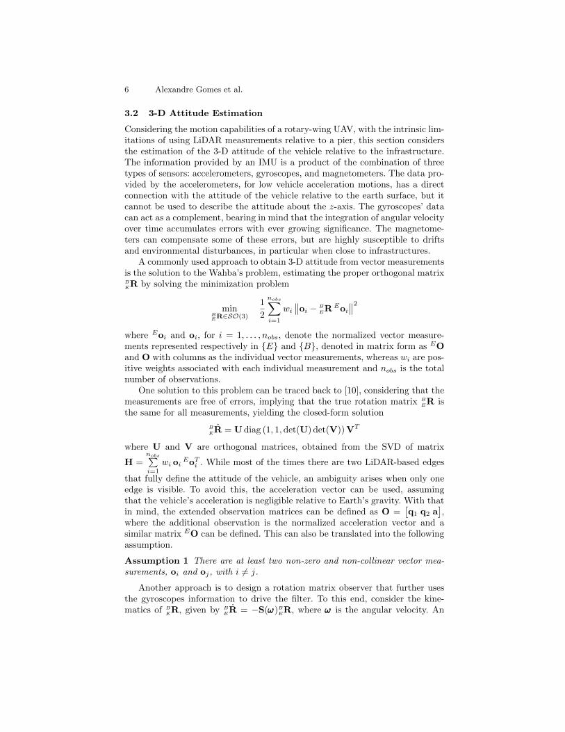
3.2 3-D Attitude Estimation

Considering the motion capabilities of a rotary-wing UAV, with the intrinsic lim-itations of using LiDAR measurements relative to a pier, this section considersthe estimation of the 3-D attitude of the vehicle relative to the infrastructure.The information provided by an IMU is a product of the combination of threetypes of sensors: accelerometers, gyroscopes, and magnetometers. The data pro-vided by the accelerometers, for low vehicle acceleration motions, has a directconnection with the attitude of the vehicle relative to the earth surface, but itcannot be used to describe the attitude about the z-axis. The gyroscopes’ datacan act as a complement, bearing in mind that the integration of angular velocityover time accumulates errors with ever growing significance. The magnetome-ters can compensate some of these errors, but are highly susceptible to driftsand environmental disturbances, in particular when close to infrastructures.

A commonly used approach to obtain 3-D attitude from vector measurementsis the solution to the Wahba’s problem, estimating the proper orthogonal matrixBER by solving the minimization problem

minBER∈SO(3)

1

2

nobs∑i=1

wi∥∥oi − B

EREoi∥∥2

where Eoi and oi, for i = 1, . . . , nobs, denote the normalized vector measure-ments represented respectively in {E} and {B}, denoted in matrix form as EOand O with columns as the individual vector measurements, whereas wi are pos-itive weights associated with each individual measurement and nobs is the totalnumber of observations.

One solution to this problem can be traced back to [10], considering that themeasurements are free of errors, implying that the true rotation matrix B

ER isthe same for all measurements, yielding the closed-form solution

B

ER = U diag (1, 1,det(U) det(V)) VT

where U and V are orthogonal matrices, obtained from the SVD of matrix

H =nobs∑i=1

wi oiEoTi . While most of the times there are two LiDAR-based edges

that fully define the attitude of the vehicle, an ambiguity arises when only oneedge is visible. To avoid this, the acceleration vector can be used, assumingthat the vehicle’s acceleration is negligible relative to Earth’s gravity. With thatin mind, the extended observation matrices can be defined as O =

[q1 q2 a

],

where the additional observation is the normalized acceleration vector and asimilar matrix EO can be defined. This can also be translated into the followingassumption.

Assumption 1 There are at least two non-zero and non-collinear vector mea-surements, oi and oj, with i 6= j.

Another approach is to design a rotation matrix observer that further usesthe gyroscopes information to drive the filter. To this end, consider the kine-matics of B

ER, given by BER = −S(ωωω)B

ER, where ωωω is the angular velocity. An


observer for BER replicates this structure, as B

E

˙R = −S(ωωω)B

ER, where ωωω is yetto be determined. As such, the error between the true rotation matrix and itsestimate can be defined as R = B

ER BERT , resulting in the error dynamics

˙R = R S(ωωω)− S(ωωω) R (1)

for which the stability of the equilibrium point R = I3 is stated in the followingresult.

Theorem 1. Considering the error dynamics in (1), let ωωω be defined as

ωωω = ωωω + kobs

nobs∑i=1

S(oi)RToi (2)

with kobs > 0. Under Assumption 1, the equilibrium point R = I3 is almostglobally asymptotically stable.

Proof. For the proof outline, let the candidate Lyapunov funcion be defined as

V (R) = tr(I3 − R

)(3)

where I3 is the identity matrix. It can easily be seen that this function is positivedefinite and vanishes at the equilibrium point, as V (R) > 0 for all R ∈ SO(3) \I3 and V (I3) = 0. After replacing (2) and some algebraic manipulation, thederivative of (3) can be written as

V (R) = −kobs2

nobs∑i=1

∥∥∥(I3 − R2)oi

∥∥∥2 .Considering Assumption 1, it can be seen that V (R) ≤ 0 for all R ∈ SO(3) andthat V (R) = 0 if and only if R = I3 and R = rot(π,n), for all n ∈ S2, where thenotation rot(θ,n) denotes a rotation about the unitary vector n of an angle θ.As such, it can be shown that the error system is almost globally asymptoticallystable, meaning that the region of attraction covers all of SO(3), except for azero measure set of initial conditions, following the approach in [2, 1]. ut

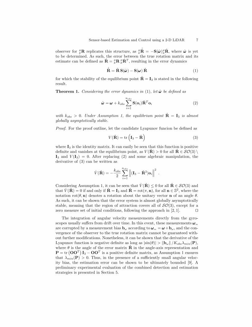
The integration of angular velocity measurements directly from the gyro-scopes usually suffers from drift over time. In this event, these measurements ωωωm

are corrupted by a measurement bias bω according to ωωωm = ωωω+bω, and the con-vergence of the observer to the true rotation matrix cannot be guaranteed with-out further modifications. Nonetheless, it can be shown that the derivative of theLyapunov function is negative definite as long as |sin(θ)| > ‖bω‖ /Kobsλmin(P),where θ is the angle of the error matrix R in the angle-axis representation andP = tr

(OOT

)I3 −OOT is a positive definite matrix, as Assumption 1 ensures

that λmin(P) > 0. Thus, in the presence of a sufficiently small angular veloc-ity bias, the estimation error can be shown to be ultimately bounded [9]. Apreliminary experimental evaluation of the combined detection and estimationstrategies is presented in Section 5.


4 Trajectory Tracking Control

This section addresses the combination of the detection and estimation strategiesand the design of controllers, aiming at tracking a trajectory defined relatively toa structure using only an IMU and a 2-D LiDAR. A nonlinear position controlleris considered, for which the simplification of the force balance that describes thevehicle can be defined by the error dynamics

˙p = Ep − Epd = Ev − Evd

˙v = Ev − Evd = ge3 − Tmr3 − Evd

˙r3 = r3 − r3d = −S(r3)RTΠe3ωωω − r3d

(4)

where m is the vehicle mass, g is the gravitational acceleration, Ep, Ev, r3, andT are respectively the vehicle’s position, velocity, third column of the rotationmatrix R = E

BR, and the thrust input, whereas Epd, Evd, r3d , and Td are theirrespective desired values. In these error dynamics, only the first two elements of

the angular velocity are used as inputs, denoted as Πe3ωωω =

[ωx ωy 0

]T, leaving

the angular motion about the vehicle’s z-axis as an extra degree of freedom. Analternative input ωωω can also be defined for simplicity as Πe3

ωωω = −RS(r3)2ωωω .The approach to stabilize this nonlinear system consists of first stabilizing the

position and velocity outer-loop driven by r3d and Td, introducing a new state

x =[pT vT

]T, and then using backstepping techniques to drive the attitude

and trust to the desired values using the vehicle thrust and part of the angu-lar velocity vector. The following result provides the conditions for asymptoticstability of the closed-loop system, assuming full state feedback.

Theorem 2. Consider the error dynamics (4), for which the feedback law ischosen as T = Td rT3 r3d , r3d = m

Tdf , Td = m ‖f‖, with the alternative input ωωω

defined as

ωωω =1

‖f‖S(r3d)f − S(r3)

[2Tdm

(P12 p + P22v) +Kr3 r3

](5)

and f = ge3 − Evd + Kp p + Kv v, f = −Evd + Kp˙p + Kv

˙v, while P12 andP22 are constant design matrices, and Kr3 > 0 is a controller gain. Then theclosed-loop system is asymptotically stable.

Proof. The proof outline for this strategy starts by defining the Lyapunov func-tion candidate

V (p, v, r3) = xTPx +1

2rT3 r3

where P is a symmetric positive definite matrix. The constant design matricesP12 and P22 from 2 correspond to the blocks of P that are relevant to thecontrol task, depending only on the position and linear velocity gains, Kp andKv . Using (5), after some agebraic manipulation, the derivative of this functioncorresponds to

V (p, v, r3) = −xTQx−Kr3 ‖S(r3)r3‖2 (6)


Overall Controller

Vehicle Simulation Sensors Simulation Detection and Estimation

HeadingController

PositionController

Saturation QuadcopterDynamics

AttitudeKinematics

LiDAR andIMU Data

EdgeKinematics

AttitudeObserver

αpiercd

ppierc

Epd

Evd

Evd

Evd

ωz

ωx

ωy

T

u T

ωωω

R

EpB

Eppier

R

pi qi

Eqi

ωωω , a

ppierc

ppierc

R

R

Fig. 3. Block diagram of the overall architecture.

(a) Vehicle and pier (b) Control Console

Fig. 4. Experimental setup at ISR/IST.

where Q is a positive definite matrix. Therefore, the derivative (6) is composedof only negative definite terms leading to asymptotic stability guarantees. ut

The remaining degree of freedom can be tackled using a simple heading lockcontroller, with the objective of maintaining a certain heading relative to thepier. A first order model of the yaw kinematics can be easily obtained using aproportional controller, resulting in a closed-loop defined as Tψ ωz = −ωz +ωzd,where Tψ is the time constant of the system. As such, the input to the system

dynamics can now be defined as u =[ωx ωy ωz T

]T. The overall architecture of

the proposed approach is presented in Fig. 3, where the controller, the simulatedvehicle and LiDAR sensor, the detection, and the attitude estimation blocks canbe identified.

5 Results

This section presents some experimental results regarding both the estimationalgorithms and the overall controlled system. The vehicle used in these trialsis based on the Mikrokopter Quadro XL, as shown in Fig. 4a, customized atISR/IST to feature a Hokuyo LiDAR UTM30LX, a Microstrain IMU, a Gumstixmini PC, among other sensors. The detection and control algorithms were ran onboard the vehicle, while a ROS-based control console was used to switch betweencontrol modes and monitor the experiments, depicted in Fig. 4b.


0 10 20 30 40 50 60

Time [s]

-10

-8

-6

-4

-2

0

2

4

6

8

10

Rol

l Ang

le [d

eg]

IMUWPARMO

0 10 20 30 40 50 60

Time [s]

-6

-4

-2

0

2

4

6

Pitc

h A

ngle

[deg

]

IMUWPARMO

0 10 20 30 40 50 60

Time [s]

10

20

30

40

50

60

70

80

Yaw

Ang

le [d

eg]

IMUYEWPARMO

Fig. 5. Attitude determination experiments, featuring results from the IMU, the yawestimation (YE), the Wahba’s solution (WPA), and the nonlinear observer (RMO).

5.1 Estimation

Regarding the attitude estimation results, the described algorithms were testedusing experimental data to assess the impact of the sensor’s noise and the ef-fectiveness of the data treatment, as shown in Fig. 5. It can be seen that boththe yaw estimator (YE) and the solution to the Wahba’s problem (WPA) aremore prone to the measurement noise than the nonlinear rotation matrix ob-server (RMO) or the IMU internal filter. As such, the rotation matrix observerobtains the best results, where the attitude description obtained in the experi-ments can be seen as a filtered version of the previous methods, maintaining asimilar proximity to the reference.

It can also be seen that the roll and pitch estimates provided by the observerhave an offset relative to the attitude obtained from the IMU. This is a resultfrom the precision of the LiDAR sensor on detecting the edges of the pier, moreparticularly, the end or length of each edge. It should also be noted that theoscillation in the YE and WPA methods are directly related to the uncertaintieswhile determining the length of the edges. Moreover, all estimation methodspresented a yaw motion description very similar among themselves and to whatwas observed in reality. In some cases not included in this paper due to spaceconstraints, the IMU yaw measurements where severely biased, probably dueto magnetic interference, while the proposed methods remained immune to thisproblem.

5.2 Control

The overall closed-loop system was implemented as presented in Fig. 3 and exper-imentally tested. The results of this preliminary experimental trial are presented


0 10 20 30 40 50 60 70 80 90

Time [s]

-3

-2.5

-2

-1.5

-1

-0.5

0

Pos

ition

[m] a

nd R

elat

ive

Hea

ding

[rad

]

xd

xy

d

yz

d

z

d

(a) Position and relative heading

0 10 20 30 40 50 60 70 80 90

Time [s]

-30

-20

-10

0

10

20

30

Act

uatio

n

x [º]

y [º]

z [º]

T [N]

(b) Actuation

Fig. 6. Experimental results of the closed-loop system, using a step reference.

in Fig. 6, where the position, heading, and actuation signals are show, consider-ing a reference with steps in position relative to the pier. It can be seen that thevehicle is able to track the reference with fair accuracy, although there is stillmargin for gain adjustment towards a more accurate trajectory tracking. At thesame time, the vehicle actively maintains the relative heading pointing towardsthe pier, even when the position of the vehicle switches between two points.

6 Concluding Remarks

This paper proposes a solution to the problem of laser-based control of rotary-wing UAVs, considering the entire process comprising the acquisition and treat-ment of the sensor’s measurements, the development of methods to computethe relevant quantities to describe the motion of the vehicle, and the designand implementation of stable and effective observers and controllers within thescope of Lyapunov stability methods. The proposed algorithms where tested inpreliminary experimental trials, allowing to validate their effective applicabil-ity to the envisioned scenarios. Future work will focus on further experimentaltests of the trajectory tracking controller and attitude observer, as well as in thedevelopment of more reliable, robust, and stable observers and path-followingcontrollers.

Acknowledgments

This work was partly funded by the Macao Science and Technology DevelopmentFund (FDCT) through Grant FDCT/048/2014/A1, by the project MYRG2015-00127-FST of the University of Macau, by LARSyS project FCT:UID/EEA/-50009/2013, and by the European Union’s Horizon 2020 programme (grant No731667, MULTIDRONE). The work of Bruno Guerreiro was supported by theFCT Post-doc Grant SFRH/BPD/110416/2015, whereas the work of Rita Cunhawas funded by the FCT Investigator Programme IF/00921/2013. This publi-cation reflects the authors’ views only, and the European Commission is notresponsible for any use that may be made of the information it contains. The


authors express their gratitude to the DSOR team, in particular to B. Gomes,for helping with the experimental trials.

References

1. Bras, S., Cunha, R., Silvestre, C.J., Oliveira, P.J.: Nonlinear attitude observerbased on range and inertial measurements. Control Systems Technology, IEEETransactions on 21(5), 1889–1897 (2013)

2. Cunha, R.: Advanced motion control for autonomous air vehicles. Ph.D. thesis, In-stituto Superior Tecnico, Universidade Tecnica de Lisboa, Lisbon, Portugal (2007)

3. Franke, U.E.: Civilian drones: Fixing an image problem? ISNBlog, ETH Zurich (2015). URL http://isnblog.ethz.ch/security/civilian-drones-fixing-an-image-problem

4. Gomes, A.: Laser-based control of rotary-wing UAVs. Master’s thesis, AerospaceEng., Instituto Superior Tecnico (2015)

5. Groenwall, C.A., Millnert, M.C.: Vehicle size and orientation estimation using geo-metric fitting. In: Aerospace/Defense Sensing, Simulation, and Controls, pp. 412–423. International Society for Optics and Photonics (2001)

6. Guerreiro, B.J., Batista, P., Silvestre, C., Oliveira, P.: Globally asymptoticallystable sensor-based simultaneous localization and mapping. IEEE Transactions onRobotics 29(6) (2013). DOI https://doi.org/10.1109/TRO.2013.2273838

7. Guerreiro, B.J., Silvestre, C., Cunha, R., Cabecinhas, D.: Lidar-based control ofautonomous rotorcraft for the inspection of pier-like structures. IEEE Transactionsin Control Systems Technology (2017). DOI https://doi.org/10.1109/TCST.2017.2705058

8. He, R., Prentice, S., Roy, N.: Planning in information space for a quadrotor he-licopter in a GPS-denied environment. In: IEEE International Conference onRobotics and Automation, pp. 1814–1820. Pasadena, CA, USA (2008)

9. Khalil, H.K., Grizzle, J.: Nonlinear systems, vol. 3. Prentice hall New Jersey (1996)10. Markley, F.L.: Attitude determination using vector observations and the singular

value decomposition. The Journal of the Astronautical Sciences 36(3), 245–258(1988)

11. Nguyen, V., Martinelli, A., Tomatis, N., Siegwart, R.: A comparison of line ex-traction algorithms using 2d laser rangefinder for indoor mobile robotics. In: In-ternational Conference on Intelligent Robots and Systems (IROS), pp. 1929–1934.IEEE (2005)

12. Pavlidis, T., Horowitz, S.L.: Segmentation of plane curves. IEEE transactions onComputers 23(8), 860–870 (1974)

13. Shapiro, L., Stockman, G.C.: Computer vision. 2001. ed: Prentice Hall (2001)14. Teixido, M., Palleja, T., Font, D., Tresanchez, M., Moreno, J., Palacın, J.: Two-

dimensional radial laser scanning for circular marker detection and external mobilerobot tracking. Sensors 12(12), 16,482–16,497 (2012)

15. Thrun, S., Fox, D., Burgard, W., Dellaert, F.: Robust Monte Carlo localization formobile robots. Artificial Intelligence 128(1-2), 99–141 (2001)

16. Tice, B.P.: Unmanned aerial vehicles - the force multiplier of the 1990s. AirpowerJournal (1991)

17. Wu, C.: Towards linear-time incremental structure from motion. In: InternationalConference on 3D Vision-3DV, IEEE, pp. 127–134 (2013)

sensor-based 3-d pose estimation and control of rotary...

Documents