sensitivity and uncertainty analysis of...
TRANSCRIPT

1
SENSITIVITY AND UNCERTAINTY ANALYSIS OF TOPMODEL FOR THE HYDROLOGICAL SIMULATION OF THE GRISE RIVER CATCHMENT
By
JOSEPH ANTOINE BENECHE
A THESIS PRESENTED TO THE GRADUATE SCHOOL OF THE UNIVERSITY OF FLORIDA IN PARTIAL FULFILLMENT
OF THE REQUIREMENTS FOR THE DEGREE OF MASTER OF SCIENCE
UNIVERSITY OF FLORIDA
2013

2
© 2013 Joseph Antoine Beneche

3
To my family and the memory of my brother, Pierre Jonas Beneche

4
ACKNOWLEDGMENTS
First, I am very grateful to Dr. Christopher Martinez, for his guidance. Without his
help I would not be able to complete my degree.
Thank you to Dr. Rafael Muñoz-Carpena and Dr. William Wise for their advice and
for accepting to be on my Committee
Thanks to the WINNER/USAID (Watershed Initiative for National Natural
Resources) project for funding my study.
Many thanks to Di Tian, Yogesh Khare, Dr. Delva, Ing. Ivelt Chery and everyone
who has helped during the entire process, from the application for the scholarship to the
completion of the degree.

5
TABLE OF CONTENTS page
ACKNOWLEDGMENTS .................................................................................................. 4
LIST OF TABLES ............................................................................................................ 8
LIST OF FIGURES .......................................................................................................... 9
LIST OF ABBREVIATIONS ........................................................................................... 11
ABSTRACT ................................................................................................................... 12
CHAPTER
1 INTRODUCTION .................................................................................................... 14
Problem Statement ................................................................................................. 14
Objectives ............................................................................................................... 17
2 LITERATURE REVIEW .......................................................................................... 18
Hydrological Modeling............................................................................................. 18
Model Classification ................................................................................................ 18 Deterministic Versus Stochastic Models........................................................... 18
Lumped Versus Distributed Models .................................................................. 19
Runoff Generation Mechanisms ............................................................................. 19
Infiltration Excess Overland Flow ..................................................................... 20 Spatial Area Infiltration Excess Overland Flow ................................................. 20 Saturation Excess Overland Flow .................................................................... 20
Subsurface Stormflow ...................................................................................... 21 Hydrological Response Process ............................................................................. 21
Characterization of the Hydrological Response ................................................ 21 Transformation of Rainfall in Hydrograph ......................................................... 22
Production function .................................................................................... 22
Transfer function ........................................................................................ 24 Sensitivity Analysis in Hydrological Modeling ......................................................... 27
Sensitivity Analysis Method .............................................................................. 28 Local SA (LSA) .......................................................................................... 28
Global sensitivity analysis (GSA) ............................................................... 29 Uncertainty Analysis in Hydrological Modeling ....................................................... 31
3 WATERSHED PRESENTATION ............................................................................ 35
Watershed Location ................................................................................................ 35 Physical Characteristics of the Watershed .............................................................. 36
Hydrology and Hydrogeology ........................................................................... 36

6
Climatology ....................................................................................................... 37
Geomorphology and Soils ................................................................................ 37 Vegetation and Land Use ................................................................................. 38
4 MODEL PRESENTATION ...................................................................................... 48
Model Scope ........................................................................................................... 48 Basic TOPMODEL Equations ................................................................................. 49 Assumptions ........................................................................................................... 52 Differences of TOPMODEL’s Versions ................................................................... 52
Model Applicability .................................................................................................. 53 Model Inputs ........................................................................................................... 53 TOPMODEL Parameters ........................................................................................ 54 TOPMODEL Parameters Sensitivity ....................................................................... 55
Topographic Index .................................................................................................. 57 Output of TOPMODEL ............................................................................................ 57
5 METHODOLOGY ................................................................................................... 59
Sensitivity Analysis ................................................................................................. 59
Sensitivity Analysis Process ................................................................................... 59 Determination of Probability Distribution Functions (PDFs) of Input
Parameters .................................................................................................... 59
Generation of Input Factor Samples ................................................................. 66 Computation of the Model Output for Each Scenario ....................................... 67
Analysis of the Output Distribution ................................................................... 68 Data Elevation Model (DEM) .................................................................................. 69
Topographic Index .................................................................................................. 69 Data ........................................................................................................................ 70 Model Run .............................................................................................................. 70
6 RESULTS AND DISCUSSIONS ............................................................................. 79
Model Justification for the Watershed ..................................................................... 79
DEM of the Catchment............................................................................................ 79 Topographic Index Results ..................................................................................... 80 Sensitivity Analysis ................................................................................................. 81
Local Sensitivity Analysis (OAT) ....................................................................... 81 Global Sensitivity Analysis ................................................................................ 82
Morris sensitivity analysis........................................................................... 83 FAST sensitivity analysis ........................................................................... 86
Discussions of the Parameters Impacts ........................................................... 89 The m parameter ....................................................................................... 89
The SrMax parameter .................................................................................. 90 The ks parameter ....................................................................................... 91 The vr parameter ....................................................................................... 92 The parameters td and CD......................................................................... 92

7
Discussions of the Sensitivity Analysis Results ................................................ 93
FAST Uncertainties ................................................................................................. 93
7 CONCLUSIONS AND RECOMMENDATIONS ..................................................... 113
Conclusions .......................................................................................................... 113 Recommendations ................................................................................................ 116
APPENDIX
A MORRIS CODE IN R ............................................................................................ 118
B FAST CODE IN R ................................................................................................. 122
C MATLAB CODE .................................................................................................... 126
D PARAMETERS CALCULATIONS ......................................................................... 141
LIST OF REFERENCES ............................................................................................. 142
BIOGRAPHICAL SKETCH .......................................................................................... 150

8
LIST OF TABLES
Table page 3-1 Slope classification in the watershed .................................................................. 39
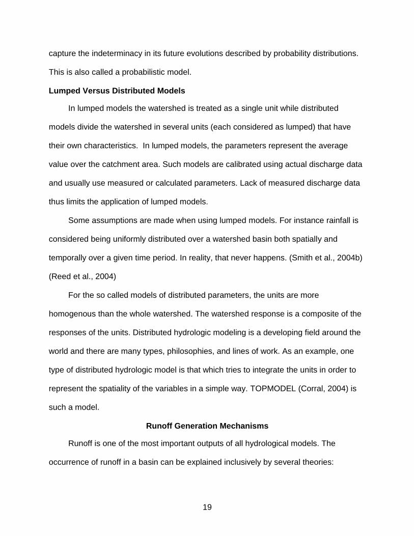
3-2 Soil properties in the catchment based on ASCE (American Society of Civil Engineers) .......................................................................................................... 40
3-3 Saturated Hydraulic Conductivity classified by USDA Soil Texture (Rawls, 1998 ................................................................................................................... 41
5-1 Summary statistics of CD (cm) parameter for various soil types ........................ 71
5-2 TOPMODEL parameters and their values for GSA ............................................ 72
5-3 TOPMODEL parameters and their values for LSA ............................................. 73
6-1 Three (3) hours sensitivity Indexes for the Morris Analysis ................................ 95
6-2 Three (3) hours sensitivity Indexes for the FAST First-Order Analysis ............... 96
6-3 Three (3) hours sensitivity Indexes for the FAST Total-Order Analysis .............. 97
6-4 Uncertainty analysis statistics for probability distributions obtained from the FAST results ....................................................................................................... 98

9
LIST OF FIGURES
Figure page 2-1 Hydrological response of a catchment (Musy, 2001) .......................................... 33
2-2 Land Use and Hydrological response. From Sauchyn (s. d.). ............................ 34
2-3 Hydrological response of a catchment (Musy, 2001) .......................................... 34
3-1 Grise River catchment location ........................................................................... 42
3-2 Towns overlapped by the catchment .................................................................. 43
3-3 Grise River in dry season view ........................................................................... 44
3-4 Hydrographic network ......................................................................................... 45
3-5 River Grise left bank ........................................................................................... 46
3-6 Grise River catchment land use .......................................................................... 47
4-1 The relation between topography, topographic index ad soil moisture deficit ..... 58
5-1 Decrease of the hydraulic conductivity with average depth ................................ 74
5-2 Derivation of an estimate of parameter m using recession curve analysis under exponential transmissivity profile assumption (Beven, 2001) ................... 75
5-3 Recession curve for the third week of December, 2011 ..................................... 75
5-4 Recession curve for the first two weeks of January, 2012 .................................. 76
5-5 Bridge of Croix des Missions in dry seasons ...................................................... 76
5-6 Bridge of Croix des Missions in rainy seasons ................................................... 77
5-7 Shape of the channel at the stages gauge ......................................................... 77
5-8 Distribution of the channel velocity inside the catchment ................................... 78
6-1 DEM of the River Grise catchment ..................................................................... 99
6-2 Map of the area processed by R-TOPMODEL ................................................. 100
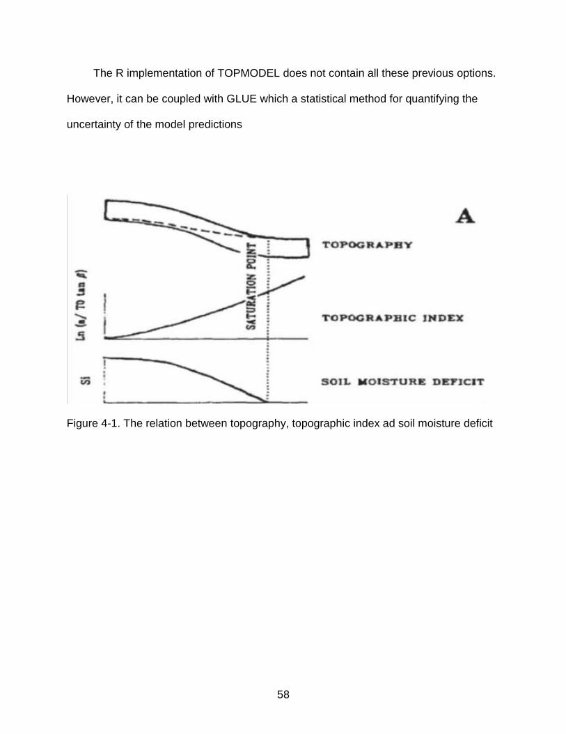
6-3 Areal distribution of the Topographic Index ...................................................... 101
6-4 OAT sensitivity of the parameters for the minimum flows ................................. 102

10
6-5 OAT sensitivity of the parameters for the Median flows .................................... 102
6-6 OAT sensitivity of the parameters for the Average flows .................................. 103
6-7 OAT sensitivity of the parameters for the Maximum flows ................................ 103
6-8 OAT sensitivity of the parameters for the Total flows ....................................... 104
6-9 Morris Sensitivity Index of the parameters for the minimum flows .................... 105
6-10 Morris Sensitivity Index of the parameters for the Median flows ....................... 105
6-11 Morris Sensitivity Index of the parameters for the Average flows ..................... 106
6-12 Morris Sensitivity Index of the parameters for the maximum flows ................... 106
6-13 Morris Sensitivity Index of the parameters for the Total flows .......................... 107
6-14 FAST Sensitivity for the Total order indexes of the parameters........................ 108
6-15 FAST Sensitivity for the First order indexes of the parameters......................... 108
6-16 FAST Sensitivity for the interactions of the parameters .................................... 109
6-17 Probability distribution of the mimimum flows ................................................... 110
6-18 Probability distribution of the median flows ....................................................... 110
6-19 Probability distribution of the average flows ..................................................... 111
6-20 Probability distribution of the maximum flows ................................................... 111
6-21 Probability distribution of the total flows ............................................................ 112

11
LIST OF ABBREVIATIONS
ASCE American Society of Civil Engineers
ASCII American Standard Code for Information Interchange
ASTER Advanced Spaceborne Thermal Emission and Reflection Radiometer
CD Capillary Drive
CDF Cumulative Distribution Frequency
CN Curve Number.
CNIGS Centre Nationale de l’Information GeoSpatiale
DEM Data Elevation Model
FAO Food and Agriculture Organization
FAST Fourier Analysis Sensitivity Test
GDEM Global Digital Elevation Model
HWSD Harmonized World Soil Database
MARNDR Ministere de L’Agriculture des Ressources Naturelles et du Developpement Rural
MOE Ministere de L’Environnment
NARR North American Regional Reanalysis
OAT One at a time
PDFs Probability Density Function
SA Sensitivity Analysis
SCS Soil Conservation System
TI topographic index
TWI Topographic Wetness Index
UNESCO United Nations Educational Scientific and Cultural Organization
USDA United State Department of Agriculture

12
Abstract of the Thesis Presented to the Graduate School of the University of Florida in Partial Fulfillment of the Requirements for the Degree of Master of Science
SENSITIVITY AND UNCERTAINTY ANALYSIS OF TOPMODEL FOR THE
HYDROLOGICAL SIMULATION OF THE GRISE RIVER CATCHMENT
By
Joseph Antoine Beneche
May 2013
Chair: Christopher Martinez Major: Agricultural and Biological Engineering
This study aimed at simulating the hydrological behavior of the Grise River
watershed which is one of the most vulnerable watersheds in Haiti. TOPMODEL was
used to perform the simulation. This is a semi-distributed model essentially based on
topography that divides the catchment into contributing areas.
Five years (1999-2002) time series of 3 hours rainfall and potential
evapotranspiration, obtained from the North American Regional Reanalysis (NARR)
project, were used for the simulation. Soil data was obtained from the Food and
Agriculture Organization (FAO) and other studies realized in this catchment. A 30m
DEM was obtained from the Advanced Spaceborne Thermal Emission and Reflection
Radiometer (ASTER) Global Digital Elevation Model (GDEM).
Both global (FAST and Morris Methods) and Local(OAT) sensitivity analyses were
performed and revealed that the decay of the decrease of transmissity with depth (m),
the logarithm of the transmissivity, the hydraulic conductivity (ks), the SrMax and the
channel flow parameter (vr) influenced the application of TOPMODEL in the River Grise
catchment in regards to diferent type of flows. Other parameters such as capillary drive
(CD) influence also the response of the watershed but on a smaller scale.

13
Ranges of variation of different types of flows were also determined in this study.
However measured data is necessary to confirm the performance of TOPMODEL in the
watershed.

14
CHAPTER 1 INTRODUCTION
Problem Statement
Scientific evidence based on long-term observations showed that climate change
and climate variability have influenced the natural resources particularly Water
resources around the world (Olivier and Hidore, 2002; Brekke, et al., 2009). Spatial and
temporal variability of rainfall and, consequently, streamflow regimes have obviously
changed. In most of the United States for example, precipitation and streamflow have
increased for the second half of the 20th century (Lettenmaier, et al., 2008). Rainfall in
West Africa has indicated a continuous decrease since 1960s while recursive anomalies
have been observed in East and North East of Africa (Moreda, 1999).
As a result of the climate variability and climate change, problems related to water
have increased. Water shortages, poor water quality and flood damages have been
increasingly observed all over the world. Parallel, population growth, agricultural
expansion to meet the food needs and industrial growth have increased the demand on
freshwater. Agriculture itself consumes 70% of the worldwide freshwater. Despite the
fact that about one third of the world’s population is actually living in either areas where
there is scarcity or shortage of water, scientific research has predicted that climate
change and variability and population growth will increase this number to one half of
humanity (United Nations Humans Development report, 2006)
Problems related to water can even be more remarkable on a watershed scale. In
addition to the global effect, local practices can have large impacts on streamflow. Land
cover and land-use changes such as residential and commercial development,

15
deforestation, reforestation, and wildfires over time can result in changes to basin runoff
patterns, which could change flood peaks, flood storage, and other uses.
Since land-use and land cover have varied and the climate change and variability
issue has become more flagrant, the integrated management and allocation of the water
resources to satisfy the needs of different sectors are the challenges decision-makers
have been facing (Simonovic, 2002). It has become urgent to link research with
improved water management. The allocation of water resources in a more efficient way
among competing needs requires a better monitoring, assessment, and forecasting of
the resources.
In this context, scientists have been looking for more efficient ways to assess the
hydrological processes within the watersheds. As a result, many hydrologic models,
which have become an essential tool for water resources planning, development, and
management, have been built to model watershed responses. Spatially distributed
rainfall–runoff models have been generated for analyzing the impact of land cover and
climate changes on streamflow regimes and surface water bodies (Harrison and
Whittington, 2002; Eckhardt and Ulbrich, 2003).
The Haitian Watersheds for example are known as some of the most vulnerable in
the world due to human activities. While only less than 30 % of the land is suitable for
farming activities (Delusca, 1998) more than 60 % of the population has lived in rural
areas using traditional farming practices that have led consequently to a drastic
decrease in water infiltration and increase in surface runoff (Dautrebande, et al., 2006).
Agricultural activities have been practicing on unsuitable steep lands.

16
Moreover, Haiti’s geographical location renders it more vulnerable. Indeed, located
on the primary pathway of tropical storms that initiate in the Atlantic and strike
Caribbean islands during hurricane season, Haiti has long been vulnerable to tropical
storms and hurricanes. However a significant increase in severe natural disasters such
as floods, hurricanes, landslides has been observed for the last decade. Flash floods
have been the most important problems the eroded watersheds have faced leading to
enormous loss of human life.
In Haiti, scientific investigation and measurement in the watersheds remain
extremely rare. This is mainly due to the scarcity of hydrologic data necessary to
conduct studies. There is been a lack of instruments capable to generate the data. The
few existing hydrologic stations enable to collect these data were installed very recently.
Some studies have been conducted to roughly estimate flood risk in some watersheds,
but there is no description of the hydrological processes that intervene in generating the
floods.
The watershed of Cul-de-Sac which encompasses the River Grise basin remains
one of the most priority Haitian watersheds, based upon the population density, the
flood risk and the vulnerability of the infrastructures (Timyan, 2006). Other authors such
as Smucker et al. (2007) and Smith et al. (2008) have confirmed this conclusion.
However none of these studies was able to quantify the hydrological processes
happening in the watershed.
Thus, this research aims to assess the hydrological response of the River Grise
basin using the TOPMODEL.

17
Objectives
The simulation of the hydrological response in this watershed with TOPMODEL
aims at determining appropriate soil and catchment factors needed to improve flood
estimation methods.
The specific objectives are:
1. Simulating the hydrological behavior of the catchment using R TOPMODEL
2. Identifying the controlling parameters of the hydrologic processes in the River Grise catchment
3. Predicting the stream discharges in the watershed

18
CHAPTER 2 LITERATURE REVIEW
Hydrological Modeling
As an important tool for hydrological system investigation, a hydrological model is
a mathematical representation of the different components of the hydrologic cycle. They
describe mathematically the elements of the water system. They have been applied on
different scales. They can be local to global; they can be more or less complex based
on the scale they are designed to address. Rainfall-runoff models have been developed
for more than thirty years based upon different concepts and perceptions. However, the
applicability of some widely accepted models may be limited by the complexity of
hydrological measurement techniques and lack of measurements in space and time.
Model Classification
There have been several ways to classify hydrological models. The two generic
classes are the deterministic versus stochastic models and the lumped versus
distributed models.
Deterministic Versus Stochastic Models
Deterministic models represent the hydrological processes based on physical
laws. They take into account no uncertainties in prediction. The variables are free from
random variation and have no probability distribution. In nature, a deterministic model is
one where the model parameters are known or assumed. On the contrary, stochastic
models account for uncertainty in model predictions due to uncertainty in input
variables, boundary conditions and /or parameter values. Instead of dealing with only
one possible reality of how the process evolves over time, stochastic models can
19
capture the indeterminacy in its future evolutions described by probability distributions.
This is also called a probabilistic model.
Lumped Versus Distributed Models
In lumped models the watershed is treated as a single unit while distributed
models divide the watershed in several units (each considered as lumped) that have
their own characteristics. In lumped models, the parameters represent the average
value over the catchment area. Such models are calibrated using actual discharge data
and usually use measured or calculated parameters. Lack of measured discharge data
thus limits the application of lumped models.
Some assumptions are made when using lumped models. For instance rainfall is
considered being uniformly distributed over a watershed basin both spatially and
temporally over a given time period. In reality, that never happens. (Smith et al., 2004b)
(Reed et al., 2004)
For the so called models of distributed parameters, the units are more
homogenous than the whole watershed. The watershed response is a composite of the
responses of the units. Distributed hydrologic modeling is a developing field around the
world and there are many types, philosophies, and lines of work. As an example, one
type of distributed hydrologic model is that which tries to integrate the units in order to
represent the spatiality of the variables in a simple way. TOPMODEL (Corral, 2004) is
such a model.
Runoff Generation Mechanisms
Runoff is one of the most important outputs of all hydrological models. The
occurrence of runoff in a basin can be explained inclusively by several theories:

20
Infiltration Excess Overland Flow
Also called Horton overland flow, this mechanism is more likely to be significant in
areas of low vegetation cover and high rainfall intensity. Horton (1933) stated that runoff
occurs when rainfall intensity exceeds infiltration or storage capacity. However, Kirkby
(1969) and Freeze (1972) remarked that in humid temperate regions covered with
vegetation infiltration capacities of soils are usually higher than normal rainfall
intensities.
Spatial Area Infiltration Excess Overland Flow
The properties of the soil vary spatially over the watershed. As a result, the
infiltration capacity of the soil is more likely to be different from one point to another.
Moreover, due to spatial variability of surface water inputs, infiltration excess runoff
does not always occur over the entire basin during a rainfall event. Betson (1964) stated
that the area contributing to infiltration excess runoff may only be a small portion of the
drainage basin.
Saturation Excess Overland Flow
This mechanism of runoff occurs when in locations where the soil profile becomes
completely saturated. In these locations, rainfall intensity does not necessarily exceed
infiltration capacity. Once complete saturation of the soil occurs at a location all further
rainfall becomes overland flow runoff (Cappus, 1960).
The complete saturation of the soil usually results in raising the water table near
the surface making stream areas susceptible to saturation from below. These areas
vary seasonally and are referred to as variable source areas (Beven 2000).

21
Subsurface Stormflow
Over relatively impermeable bedrock, water flows downslope after satisfying some
initial depression storage. This situation was pointed out by Dunne and Black in 1979.
As a result, when both the soil is deep enough and the capacity of infiltration is high, the
streamflow is dominated by the subsurface flow (Beven, 2000).
Hydrological Response Process
The hydrological response is defined as the reaction of the basin when it is
subjected to precipitation (Musy, 2005).The watershed is the basic hydrologic unit within
which all measurements, calculations and predictions are made in hydrology. The
characteristics of the watershed and the precipitation involve in expressing the
hydrological response of the watershed. It is usually measured by the amount of water
that flows at the outlet. The hydrological response can be graphically represented by the
plot of discharge in the channel versus time called a hydrograph or by the plot of the
water level versus time which is limngraph.
In fact, establishing the relationships between the physical attributes of the
catchment and the behavior of the stream or river leaving a watershed has been one of
the most important problem hydrologists have faced in watershed hydrology.
Characterization of the Hydrological Response
The hydrological response as represented in the Figure 2-1 can be characterized
in several different ways. The hydrological response can be either null or positive. This
is the case when subjected to the precipitation the stream or the river leaving the
watershed does not change. The hydrological response is, on the contrary, positive
when under the climatic stimuli the flow regime is modified.

22
As expressed in Figure 2-2 the hydrological response varies with land use. When
the hydrological response is positive, it can be fast, delayed, total or partial (Musy,
2005).
1. Fast: when the response occurs within a relatively short period of time after the catchment has been subjected to the solicitation. It is more important in case of surface flow.
2. Delayed: when the lag time is relatively long the response is considered to be delayed. It occurs when the contribution of the subsurface is more important in the runoff generation process.
3. The hydrological response is thought of as total when it is composed of both the surface and subsurface flow
4. The hydrological response is considered as partial when it results from either the surface flow or subsurface flow
Transformation of Rainfall in Hydrograph
The transformation of rainfall into hydrograph is obtained by applying successively
two functions referred to as production function and transfer function as indicated in the
Figure 2-3.
Production function
The description of the hydrological response of the watershed solicited by climatic
stimuli requires first the understanding and the estimation of flows at the interface soil-
vegetation-atmosphere. This estimation consists in determining the total losses which is
the collective term given to the various processes that act to remove water from the
incoming precipitation before it leaves the watershed as runoff (McCuen et al., 2002).
These processes are evaporation, transpiration, interception, infiltration, depression
storage, and detention storage.

23
Several techniques have been proposed for estimating the amount of rainfall lost
as abstraction form the effective rainfall that contributes to runoff. The SCS curve
number and the phi-index methods are the most frequently used.
1. The SCS method accounts for abstractions as the difference between the
volumes of rainfall and runoff. It relates runoff depth to rainfall depth. The
Equation (2-1) expresses the Runoff as computed by SCS.
(2-1)
R and P are respectively the runoff and the precipitation depth; and the maximum
watershed retention S is given in Equation (2-2).
(2-2)
CN is a runoff index called the runoff curve number.
The total loss is separated into two parts: the initial abstraction Ia and the retention.
The initial abstraction is related to CN by the empirical equation as shown in Equation
(2-3).
(2-3)
2. The phi-index method assumes a constant rate of abstraction over the duration
of the storm. These total abstraction methods simplify the calculation of storm
runoff rates (McCuen et al., 2002). Mathematically the phi-index method for
modeling losses is described by (Theodore et al., 1987) in the Equations (2-4)
and (2-5).
(2-4)
(2-5)

24
where f (t) is the loss rate; I (t) is the storm rainfall intensity; t is the time; and is the
calibration constant, called the phi index.
Transfer function
The transformation of the flows generated from different parts of the watershed
into a hydrograph at the outlet is referred to the process called Transfer function
(Hingray et al., 2009). This contribution accounts for both overland flow and interflow
(Bedient et al., 2008). There are several methods to compute the hydrograph.
1. Rational method: The Rational formula is one of the simplest formulas that
compute the prediction of peak flow. It is obtained as mentioned in the Equation (2-6)
(Bedient et al., 2008).
Qp= CiA (cfs) (2-6)
where C is the runoff coefficient. It varies with land use, i is intensity of rainfall of chosen
frequency for a duration equal to time of concentration tc (in. /hr.) tc is equilibrium time
for rainfall occurring at the most remote portion of the watershed to contribute flow at
the outlet, A is catchment area (acres).
As we can see the previous formula computes the peak flow . It does not
necessarily present the conversion of the excess flow into a hydrograph.
2. Time –area methods: One of the interesting ways to understand how rainfall
excess is converted into hydrograph is the time–area histogram. The assumption made
in this method is that the outflow hydrograph results from pure translation of direct runoff
to the outlet at uniform velocity, ignoring any storage effects in the watershed. This
method is given by the Equation (2-7) (Bedient et al., 2008).
(2-7)

25
where = hydrograph ordinate at time n (cfs), Ri is excess rainfall ordinate at time i
(ft/s) and Aj is time –area histogram ordinate at time j (ft2)
3. Unit hydrograph method: A unit hydrograph is defined as the hydrograph that
results from 1-inch (or meter) of excess precipitation (or runoff) spread uniformly in
space and time over a watershed for a given duration.
Several assumptions inherent to the Unit Hydrograph Method tend to limit its
application to any given watershed (Johnstone and Cross, 1949):
1. The duration of direct runoff is always the same for uniform-intensity storms of the same duration, regardless of the intensity
2. The direct runoff volumes produced by two different excess rainfall distributions are in the same proportion as the excess rainfall volume
3. The time distribution of the direct runoff is independent of concurrent runoff from antecedent storm events
4. Hydrologic systems are usually nonlinear due to factors such as storm origin and patterns and stream channel hydraulic properties
5. Despite this nonlinear behavior, the unit hydrograph concept is commonly used because, although it assumes linearity, it is a convenient tool to calculate hydrographs and it gives results within acceptable levels of accuracy
6. The alternative to UH theory is kinematic wave theory and distributed hydrologic models
4. Snyder’s Synthetic Unit Hydrograph: The basin lag is given in the following
Equation (2-8).
(2-8)
Ct is a coefficient ranging from 1.8 to 2.2, L is the length of the basin outlet to the basin
divide, Lc is the length along the main stream to a point nearest the basin centroid.
The Equation (2-9) expresses the peak discharge as followed
(2-9)

26
where 640 will be 2.75 for metric system, Cp is a storage coefficient ranging from 0.4 to
0.8 where larger values of Cp are associated with smaller values of Ct, A is the drainage
area.
The time base is given by the Equation (2-10).
(2-10)
However, for small watershed the time is obtained by multiplying tp by a value
ranging from 3 to 5
The duration is given by the Equation (2-11).
(2-11)
For other rainfall excess duration, the Equation (2-12) expresses the adjusted
basin lag as followed
(2-12)
The width expressed in the Equations (2-13) and (2-14) respectively for 50% and
75 % of Qp are where 770 and 440 should be replaced with 2.14 and 1.22 when the
metric unit system is used
(2-13)
(2-14)
5. SCS method: The hydrograph calculated in the Equation (2-15) is a triangle
with a rainfall duration D, time of rise Tr, time fall B and peak flow. The direct runoff is
obtained as stated in the Equation (2-16).

27
(2-15)
(2-16)
From the analysis of historical streamflow data, B is usually equal to 1.67 Tr. So the
peak discharge is calculated as stated by the Equation (2-17)
(2-17)
Sensitivity Analysis in Hydrological Modeling
Sensitivity analyses consists of determining qualitative or quantitative variation
induced in the model outputs by varying one or multiple inputs factors of the model
(Saltelli et al., 2000). Hydrologic models that are mathematical or empirical descriptions
of the watershed response to rainfall are based on conceptualization, assumptions and
hypotheses. Model inputs are subject to multiple sources of uncertainty including errors
of measurements, spatial and temporal limitations, and poor or partial understanding of
the processes involved. Accordingly, the outputs of these models can also present
imperfections that have been incorporated through hypothesis, structures, quantity and
quality of input data, and parameter estimates (Gupta et al., 1999; Satelli et al., 2000,
Muletha and Nicklow, 2005). As a result, sensitivity analyses are conducted to
determine:
1. The resemblance of the model to the system it represents
2. The factors that most influence the outputs and that particularly required stronger knowledge.
3. Parameters that are insignificant
4. Region in space where the model variation is maximum

28
5. The optimal regions within the space of input factors for use in a subsequent calibration study.
6. Factors that interact with others if there is any (Satelli et al., 2000)
The sensitivity analysis process involved following four particular steps that are:
1. Determination of probability distribution functions (PDFs) of input parameters
2. Generation of input samples
3. Model simulations to calculate desired outputs/ decision variables
4. Statistical analysis that generates sensitivity indices and parameter rankings (Saltelli et al., 2000)
Sensitivity Analysis Method
Several methods of sensitivity analysis (SA) exist that have their own strengths
and weaknesses. The choice can be difficult and depends on the problem under
investigation, the characteristics of the model and the computational cost. The methods
can be generally classified into two that are the local SA methods and the global
methods
Local SA (LSA)
Local sensitivity analysis (LSA) that is usually carried out by computing partial
derivatives is mostly concentrated on the local impact of the factors of the model. Local
analysis addresses sensitivity relative to point estimates of parameter values. The local
derivative of the desired output variable is calculated around a certain value of one input
parameter while holding other input parameters constant at their mean values. It is less
helpful when being used to compare the effect of various factors on the output.
One-At-A-Time (OAT) is one of the experiment designs of the local sensitivity
analysis (LSA). Simplest class of screening designs; it uses nominal or standard values
per factor often obtained from the literature. Two extreme values are usually used for

29
the range of likely values of each factor. The mean value of the factor which is usually
calculated or found in the literature is midway between the two extremes. A comparison
is then made between the magnitudes of the differences between the outputs for the
extreme inputs and the mean or standard value to find the factors that impact the most
the model results (Satelli et al., 2002).
Daniel (1973) classified the OAT designs into five categories:
1. Standard OAT designs that vary one factor from the standard value
2. Strict OAT designs that one factor from the standard value of the preceding experiment
3. Paired OAT designs that produce two observations and hence one simple comparison at a time
4. Free OAT designs that make each new run under new conditions
5. Curved OAT designs that produce a subset of results by varying only one-easy-to-vary factor
Global sensitivity analysis (GSA)
Global sensitivity analysis is studies how the variation in the output of a model can
be apportioned to different sources of variation, quantitatively or qualitatively in the
model inputs. Unlike LSA, Global Sensitivity Analysis methods estimate the effect of a
factor while all other factors are varied simultaneously. This variation of the other factors
accounts for interactions between variables without depending on the stipulation of a
nominal point. It describes the probability distribution function that covers the factors
ranges of existence by examining sensitivity with regard to the entire factor distributions.
Some of the global sensitivity analysis methods are the Morris Method, which is a
screening method, the Fourier Analysis Sensitivity Test method and the Sobol method
which are variance-based methods.

30
1. The Morris Method: The Morris method (Morris, 1991) tends to determine
which factors may have negligible, linear and additive or non-linear or interact with other
factors. The Morris experiment is composed of individually randomized one-factor-at-a-
time experiments (Saltelli et al., 2004). The Morris method is considered as a global
sensitivity method because it covers the entire space over which the factors can vary.
Morris computes a number r of local measures at different points and averages these
points. Morris is computationally more efficient than other methods of global sensitivity
analysis since it requires few simulations and can be interpreted easily (Saltelli et al.,
2005).
The entire domains of the factors are randomly sampled to obtain finite
distributions of elementary effects (Fi). High influence of the factors on the output results
in high mean of the distribution, whereas high standard deviation reveals there is either
interaction within factors or a non-linear effect exists (Morris, 1991; Saltelli et al., 2004).
However, the Morris method cannot give a quantitative measure about the
percentage of total output uncertainty caused by uncertainty of each parameter. The
number of simulations (N) to perform in the Morris is obtained by multiplying the
sampling size for search trajectory (r) to the number of factors (k) increased by one unit
(r*(k+1)).
2. Fourier Amplitude Sensitivity Test Method (FAST): This method has been
developed for the uncertainty and sensitivity analysis (Cukier et al., 1973, 1975, 1978).
It allows the estimation of the expected value and variance of the output variable and
the contribution of the individual input factor to the variance (Saltelli et al., 2000).

31
The Fourier Amplitude Sensitivity Test Method (FAST) presents two types of
computations. The first one is the classical FAST that computes the first-order indices
which are numbers indicating the primary effects of the factors. The second one is the
Extended FAST. It was proposed by Saltelli et al. (1999b) and measures the total effect
of the factors. It adds up the impacts of each factor and their interactions. In Extended
FAST, (Saltelli et al., 1999), the total effect is evaluated by search curve that scans the
space of the input factors in such a way that each factor is explored with selected
integer frequency.
The simulation in the FAST is obtained at of cost M*k runs, where M is a number
between 500 and 1000 and k is the number of factors.
3. The Sobol’ Method: The Sobol’ method is usually used to obtain quantitative
measures on how the uncertainty in model outputs can be apportioned to uncertainty in
individual input variables (Saltelli et al., 2000). The main idea behind the Sobol’
approach is to decompose the function into summands of increasing dimensionality
(Satelli et al., 2000). The main difference between FAST and Sobol’s method is the
approach by which the multidimensional integrals are calculated. Whereas Sobol’s
method uses a Monte Carlo integration procedure, FAST uses a pattern search based
on a sinusoidal function.
Sobol can provide all the orders of indices from first to total. The number of
simulations (N) to perform in the Sobol’ is obtained by multiplying M (a number between
500 and 1000) by the number of factors (k)
Uncertainty Analysis in Hydrological Modeling
While the sensitivity analysis tries to determine the change in model output values
that induces by changes in model input values, the uncertainty analysis attempts to

32
describe the entire set of possible outcomes. An uncertainty analysis consists in
randomly choosing input values resulting from model simulation to obtain statistical
measures of the distributions of the outputs. It is useful to determine ranges of potential
outputs of the system and probabilities associated with them. It also estimates the
probability that the output will exceed a target value. In any uncertainty analysis some
assumptions are made. Statistical distributions for the input values are considered to be
correct and the model is assumed to good enough to describe the processes taking
place in the system.
Morgan and Henrion (1992), Haan (2002), and Shirmohammadi et al. (2006)
provide extensive review of uncertainty analysis methods applied to environmental
models. First‐Order‐Approximation (FOA) (Morgan and Henrion, 1992) and the Monte
Carlo Simulations (MCS) are two methods for generating the general probability
distributions of the output variables of interest, which is the best method to quantify
model uncertainty (Haan 2002). In the first method, the expected value of the output is
obtained based on the variance and covariance of the input parameters and their local
absolute sensitivity indices. The second method is carried out by performing three
different steps: first, a random sampling of the multivariate input distribution is
performed; second the model simulations are run with the sampled values to produce
estimates of model output values; and finally a PDF is produced by combining these
output values. The procedure requires lot of computations.

33
Figure 2-1. Hydrological response of a catchment (Musy, 2001)

34
Figure 2-2. Land Use and Hydrological response. From Sauchyn (s. d.).
Figure 2-3. Hydrological response of a catchment (Musy, 2001)

35
CHAPTER 3 WATERSHED PRESENTATION
Watershed Location
This study was carried out in one of the watersheds of the metropolitan area as
presented in Figure 3-1. The River Grise basin is varied and complex basin for its
geography and its land use. This basin presents an important interest and has been
pointed out as one of the most vulnerable watersheds in the country. The inundation
risk in this catchment is really important and has been aggravated by agricultural
practices, land use and unplanned urbanization.
The study area presents three more or less different defined zones: a rural zone
lies in the upper part of the catchment; the middle part of the basin is an urban area;
and the downstream area has both urban and sub-urban areas which have been more
and more densely populated for the last decades.
The region is represented by the River Grise basin. Located in the southeastern of
Port-au-Prince, it is bordered to the south by the summit of the Massif de la Selle, to the
west by the hills and Calabasse and Gelin, to the east by the hills Mare Réseau et
Pays-Pourri, and to the north by the hills Dumay and Chacha (Georges, 2008). The
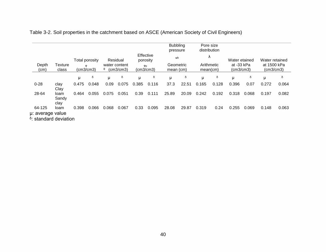
watershed straddles six municipalities as indicated in Figure 3-2 which are, in the upper
part, Kenscoff and Croix-des-Bouquets; in the middle, the Petion-Ville and Croix-des-
Bouquets; and in the lower part, Tabarre, Cite Soleil, the biggest shantytown in the
country, Delmas and Croix-des-Bouquets. The catchment covers an area of 392 km2
and is itself part of another wider watershed, Cul-de-Sac.

36
Physical Characteristics of the Watershed
The multiple interactions that have occurred in the watershed over time influence
its hydrological behavior. Occurring at the interface between the lithosphere and the
atmosphere, these interactions can be geological, climatological and meteorological etc.
Also they influence in many ways the geomorphologic factors, the soil characteristics
and the vegetation particularities, and to some extent determining the hydrology of the
catchment.
Hydrology and Hydrogeology
Several streams and springs are encountered in the River Grise catchment.
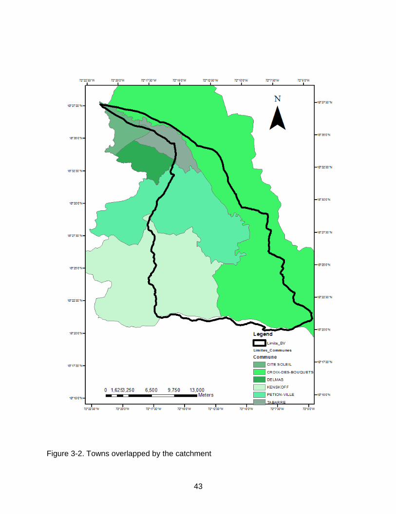
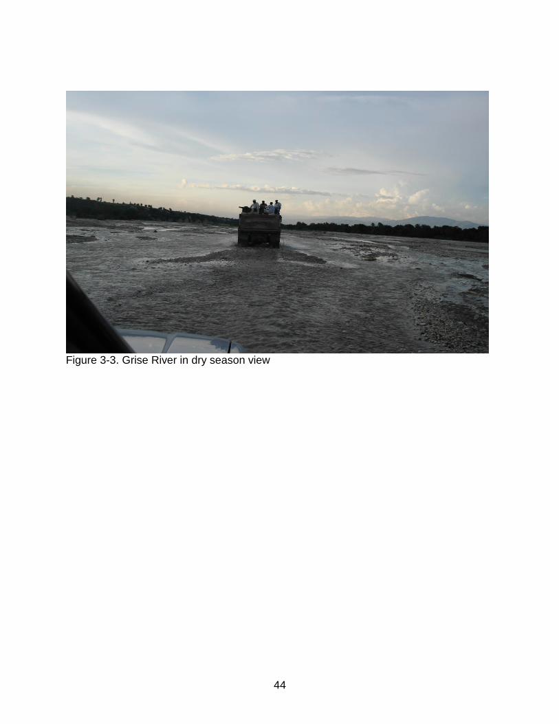
However most of them are perennial. The main river is the so called River Grise (Figure
3-3). Its name is due to the nature of the pebbles found in its bed which are from arising
basalt and limestone formations eroded in the upstream. It presents an average flow of
3.93 m3/s (MARNDR/MOE 2000).
With a wide bed and a low average flow, the River Grise is generally passable with
light vehicles or on foot most of the time. However, in rainy seasons, flooding of the
River Grise is devastating for crops and surrounding habitats. Nevertheless the regime
of the River Grise has seriously evolved over time due to deforestation. In dry periods,
the flow decreases significantly while devastating floods are becoming more frequent in
rainy seasons. It is alimented by various ravines that drain the foothills of the Massif de
La Selle. A network of ravines drains rainwater from the southern part of the watershed.
These ravines flow, for some, into the River Grise (Figure 3-4). For the others on the
contrary, the water is scattered in residential areas and roads due to lack of continuity in
this natural system to the nearby river.

37
The River Grise represents an important source of recharge for the aquifer of Cul-
de-Sac which is the main source of fresh water for the metropolitan area. Groundwater
is typically found in layers of sand and gravel with a thickness of 1 to 8 meters
separated by layers of silt and clay (Knowles et al., 1999).
Climatology
Depending on whether it is the lowland or the mountain, the climate of the Grise
River catchment varies. In Port-au-Prince, the annual rainfall averages 1300 mm while it
is around 946 mm in Croix-des-Bouquets. However, the climate is rather humid in the
upstream part of the catchment. Windward and mountainous, the annual rainfall varies
from 1450 mm in Petion-ville to 2000 mm in Kenscoff (Sergile, 1998; Holly, 1999).
Two rainy seasons are observed over the year in the study region: the first goes
from April to May and the second, from September to November. Both rainy seasons
are followed by a dry season (Holly, 1999).
Geomorphology and Soils
The geology of the region reflects the history of the island (MacFadden, 1986). In
general, five major types of soil can be observed in the vicinity of Port-au-Prince. From
oldest to later, there are massive limestone of the Eocene, sandy and marl limestone of
Miocene, Pliocene sequence, basalts and Quaternary deposits. However, two types of
geological materials are more likely to be observed: The Eocene limestone which is
mainly karst forms the mountains that limit the plain of Cul-de-Sac and constitutes 51 %
of the geology of the River Grise basin (Projet Interuniversitaire Ciblé, 2008). Generally
they are white with a content of calcium carbonate that often exceeds 90% (Figure 3-5);
Basalts (volcanic) rocks which count for 35% and the deposit materials for the
remaining (AgroConsult, 2009).

38
Alternating beds of gray marl and limestone give the formation of the Grise River.
The thickness of the formation is variable but is estimated to several hundred meters in
average (Projet Interuniversitaire Ciblé, 2008).
This catchment rather presents a mountainous configuration. In the upstream, the
altitude varies from 200 m to 2250 m with very steep slope as up to 60%. According to
CNICS, 60% of the area has a slope higher than 35% while less than 20% has a slope
between 0 % and 12 % as indicated in the Table 3-1.
Soils in the River Grise basin are a mosaic on the historical geology of the bedrock
and terrain originated from basalt, limestone and alluvium (Georges, 2008). The
Harmonized World Soil Database (HWSD) which is the soil database of the FAO
presents the properties of the soils encountered within the watershed. Cambisol is
predominant with a predominant texture of clay loam both in the topsoil and the subsoil.
The depth of the soil is an approximate of 1.25m.
Richard et al. (2004), Lalonde et al. (1977) and HWSD found approximately the
same classes of soil ranked in the Table 3-2.
Vegetation and Land Use
The vegetation varies with the difference existing in the topography of the basin
from mountain to lowland ecosystems as indicated in the Figure 3-6. The flora is very
diverse: Pine forest, hardwood forest, dry forests, humid forest of lowland etc. (Swartley
et al., 2006). This watershed had presented one of the most interesting vegetation of
the Caribbean region in terms of botany (Ekman 1926, Judd 1987, Holdridge 1947).
However, the deforestation’s effect has affected significantly the vegetation.
Agriculture remains the main use of the land of the Grise River catchment. About
42 % of the land is allocated to agriculture which can be observed almost everywhere

39
on the catchment. Savannah zones and pastures occupy respectively about 30 % and
15 % of the catchment. More or less dense forests account for 8 %.
Table 3-1. Slope classification in the watershed
Class (%) Area km2 Percentage of the catchment
0-12 75.78 19.29
12-25 50.55 12.86
25-35 26.25 6.68
> 35 240.35 61.17
Total 392.93 100.00
Source: CNIGS
40
Table 3-2. Soil properties in the catchment based on ASCE (American Society of Civil Engineers)
μ: average value ᵟ: standard deviation
Depth (cm)
Texture class
Total porosity ᵩ
(cm3/cm3)
Residual water content ᶿ (cm3/cm3)
Effective porosity
ᵩe (cm3/cm3)
Bubbling pressure
Pore size distribution
Water etained at -33 kPa (cm3/cm3)
Water retained at 1500 kPa (cm3/cm3)
ψb λ
Geometric mean (cm)
Arithmetic mean(cm)
μ ᵟ μ ᵟ μ ᵟ μ ᵟ μ ᵟ μ ᵟ μ ᵟ
0-28 clay 0.475 0.048 0.09 0.075 0.385 0.116 37.3 22.51 0.165 0.128 0.396 0.07 0.272 0.064
28-64 Clay loam 0.464 0.055 0.075 0.051 0.39 0.111 25.89 20.09 0.242 0.192 0.318 0.068 0.197 0.082
64-125
Sandy clay loam 0.398 0.066 0.068 0.067 0.33 0.095 28.08 29.87 0.319 0.24 0.255 0.069 0.148 0.063

41
Table 3-3. Saturated Hydraulic Conductivity classified by USDA Soil Texture (Rawls, 1998
USDA Soil Class Texture Saturated Hydraulic conductivity 1(k0)
(in/hr)
Range saturate Hydraulic Conductivity2 (k0) (in/hr)
Sand 5.3 10.3 - 3.6
Fine Sand 4.8 8.7 - 4.2
Loamy Sand 2.6 5.6 - 1.4
Loamy sand Fine 2.3 4.8 - 1.4
Sandy Loam 0.9 2.7 - 0.4
Fine loam Sandy 0.5 1.1 - 0.2
Loam 0.2 0.8 - 0.11
Silt Loam 0.3 0.9 - 0.14
Sandy Loam Clay 0.14 0.6 - 0.04
Clay Loam 0.05 0.28 - 0.01
Silty clay Loam 0.17 0.5 - 0.09
Sandy Clay 0.04 0.12 - 0.01
Silty clay Clay 0.06 0.28- 0.02
Clay 0.07 0.027-0.03 1 Geometric mean value from k0 database
2 25% and 75% percentile values from k0 database

42
Figure 3-1. Grise River catchment location
43
Figure 3-2. Towns overlapped by the catchment
44
Figure 3-3. Grise River in dry season view

45
Figure 3-4. Hydrographic network

46
Figure 3-5. River Grise left bank

47
Figure 3-6. Grise River catchment land use

48
CHAPTER 4 MODEL PRESENTATION
Model Scope
First developed in 1979 by Beven and Kirkby, TOPMODEL is a semi-distributed
model in which the predominant factors affecting the watershed response to
precipitation are derived from the topography of the catchment and the soil
transmissivity. The topography influences many aspects of the hydrologic system. It
defines the movement of water in the watershed under the effect of gravity (Wolock and
Price, 1994).
Divided into grid cells, the topography of the catchment is represented by means
of a topographic-soil index, ln (α/T0tanβ), where α is the area draining through the grid
square per unit length of contour; T0 is the transmissivity of the soil, β is the local
gradient of ground surface and tanβ is the average outflow gradient from the square.
When the spatial variability of the soil transmissivity is neglected, the index becomes the
topographic index ln (α/tanβ) (Quinn et al., 1991). The topographic index reflects the
spatial distribution of the soil moisture, surface saturation and runoff generation process
(Zang and Montgomery, 1994). It assigns the same index to every point hydrologically
similar. It is computed using topographic data such as DEM (Data Elevation Model).
TOPMODEL allows at most thirty (30) discrete increments of the index. The
transmissivity is computed as function of a saturated hydraulic conductivity which
decreases exponentially with the depth.
The surface runoff computation in TOPMODEL includes both saturation excess
and infiltration excess runoff (Montesinos-Barrios and Beven, 2004) using the variable
source area concept of stream flow based on the topographic Index.

49
TOPMODEL is also considered as a physically based model (Beven and Kirby,
1979, Beven et al., 1984). Its parameters can be derived based on physical laws. Some
parameters can also be measured in situ.
Basic TOPMODEL Equations
Total flow computed by TOPMODEL in the contributing area concept is measured
as the sum of the saturation overland flow and the subsurface flow. It is expressed in
the Equation (4-1).
qtotal =qoverland + qsubsurface (4-1)
Where qtotal [L/T] is the total flow per unit area, qoverland [L/T] is the saturation overland
flow per unit area, qsubsurface [L/T] the subsurface flow per unit area. Saturation overland
flow is estimated as the sum of direct rainfall on the saturated areas and return flow as
defined by the Equation (4-2).
qoverland = qdirect+ qreturn (4-2)
Where qdirect [L/T] is direct precipitation on saturated areas, and qreturn is return flow.
In TOPMODEL, the volume of water entering the soil is equivalent to the quantity
of water leaving this particular column of soil (steady-state conditions). Also, it is
assumed that the water table is recharged at a spatially uniform rate (R). The model
derives expressions to compute the flows at some location x by using the Darcy’s Law
and the continuity Equation (4-3):
AxR = TxtanβxCx (4-3)
where tanβx is the hydraulic gradient at x, Ax [L2] is the area upslope from x that drains
past the location, Tx [L2/T] is the transmissivity of the saturated thickness at the location
x, and Cx [L] is the contour width at x traversed by subsurface flow.

50
Beven and Kirkby (1979) assume that soil transmissivity at the saturated thickness
x is a function of the hydraulic conductivity, which decreases exponentially with depth.
The soil surface is generally permeable because aggregations create flow pathways.
Mathematically, the diminution of the transmissivity with depth is written as in the
Equation (4.4).
(4-4)
Where zwt is the depth to the water table and the hydraulic conductivity at the soil
surface and f is the decay parameter for the decrease of hydraulic conductivity with
depth.
By substituting Tx in equation (4-3) and dividing by Cx, zwt is integrated to obtaining
the average depth to the water table as expressed in the Equation (4-5).
(4-5)
Then 𝜆, ax and T0 are respectively obtained in the Equations (4-6), (4-7) and (4-8)
(4-6)
(4-7)
(4-8)
TOPMODEL ‘s equations can be usually expressed in terms of saturation deficit
(S) which is the product of the depth to the water table and readily drained soil porosity
(θ). By multiplying the Equation (4-5) by θ we obtain the Equation (4-9):
(4-9)
And m is obtained in the Equation (4-10)

51
(4-10) Equation 4-9 states that the saturation deficit at any location x is determined by the
watershed average saturation deficit (S) and the difference between the mean of the 𝜆
and the value of
The location x in the watershed where Sx ≤ 0 is considered as saturated and can
generate saturation overland flow; any location where Sx < 0 produces return flow. The
value of qdirect is obtained by adding the products of the saturated areas ax by the
precipitation intensity, i, and dividing by the watershed area, A, as presented in the
Equation (4-11).
(4-11)
Where Sx ≤ 0.
The value of qreturn is computed by summing the products of the saturated areas
and the absolute value of their saturation deficits which are negative, divided by the total
area as indicated in the Equation (4-12):
(4-12)
Where Sx < 0.
Subsurface flow, qsubsurface, is computed by combining Darcy’s Law for saturated
subsurface flux (q x), (the right-hand side of equation 4-3 divided by Cx) with equation 4-
4, the expression for transmissivity of the saturated thickness, along the derived values
of zwt and m to obtain the Equation (4-13):
(4-13)

52
By integrating the previous equation along the length of all stream channels we
obtain the Equation (4-14).
(4-14)
Assumptions
The structure of the TOPMODEL is underpinned by some basic assumptions:
Steady-state is assumed to estimate the dynamics of the saturated zone
1. The hydraulic gradient of the saturated zone can be estimated by the local
surface topographic slope, tanβ; and groundwater table and saturated flow are
parallel to the local surface slope.
2. The transmissivity decreases with depth as an exponential function of storage
deficit or depth to the water table.
3. Hydraulic similarity is assigned to the grid cells with the same topographic index.
Differences of TOPMODEL’s Versions
Initiated by Professor Mike Kirkby at the School of Geography at the University of
Leeds in 1974, TOPMODEL has been varied in different versions with varying levels of
complexity. Some versions of TOPMODEL compute snowmelt and snow-accumulation
(Wolock and others, 1989) whereas others do not (Wood and others, 1988). All the
different versions of TOPMODEL do not include all the concepts of streamflow
generation. For example, while some computes both infiltration excess overland flow
and the variable-source-area of streamflow generation (Wolock, 1993),
evapotranspiration estimation can vary from one version to another. Evapotranspiration
is estimated in some versions based on empirical computations whereas others use
physically based methods to compute evapotranspiration (Famiglietti, 1992).

53
It is also noticeable that the level of spatial complexity and aggregation of the input
and processes simulation differ from among the versions of TOPMODEL.
Model Applicability
TOPMODEL was first generated for the simulation of humid catchments in the
United Kingdom (Beven and Kirkby, 1979; Beven et al., 1984, Quinn and Beven, 1993),
in the eastern part of the United States of America (Beven and Wood, 1983, Homberger
et al., 1985) and Scotland (Robson et al., 1993). The model has performed well for flow
rates simulations and spatially distribution of saturations.
However, for the last decades several attempts have been made to simulate the
hydrological responses of catchments located under more or less dry conditions.
TOPMODEL was successfully applied to forecast flood in various Southern France
catchments according to Durand et al., (1992), Sempere-Torres (1990) and Wedling
(1992). TOPMODEL has also given good results for its applications to some Spanish
basins (Piñol et al., 1997).
However, according to Seibert et al. (1997), TOPMODEL is not capable of
producing the correct dynamics for groundwater, and consequently its ability to simulate
runoff in shallow watersheds is reduced. In fact, the assumptions of spatial uniform
recharge and steady flow rates are too simple. Measurements in different catchments
showed that groundwater responses to storms can present wide spatial variations
Model Inputs
Discharge and spatial soil water saturation pattern are simulated in TOPMODEL
based on hydrological data time series and topographic information. The R
implementation of TOPMODEL which is used in this study requires observed rainfall,
potential evapotranspiration and the catchment topographic index map(Buytaert et al.,

54
2005). The Topographic Index is generated from the Data Elevation Model (DEM) using
such tools as GIS or other specific programs released with TOPMODEL.
However, in order to calibrate the simulation TOPMODEL observed discharge is
also needed.
TOPMODEL Parameters
The quantity of parameters required to run TOPMODEL depends on the version of
the model that is being used. All of the TOPMODEL versions use at least five
parameters. Some versions however have up to twelve parameters.
The following are the parameters usually used in TOPMODEL and also the ones
that are used in the R implementation:
1. m: Also named scaling parameter, it controls the decrease of transmissivity with
depth and the shape of the hydrograph recession. Kinner and Stallard (1999)
observed that 63%of the transmissivity is within 1m and 86 % is within 2m. It has
a length unit [L]
2. SrMax : is the maximum moisture deficit in the root-zone. It physically occurs when
the canopy is dry and the soil is the wilting point. It has a length unit [L]
3. td: Unsaturated zone time delay per unit storage deficit. When water is added to
the root-zone, the deficit decreases until zero, and then water is added to the
unsaturated zone becoming unsaturated zone storage. It has a length unit [T/L]
4. Sr: initial root zone deficit. When it is null, evapotranspiration occurs at potential
rates. It has a length unit [L]
5. LnTe: is the natural logarithm of the effective transmissivity of the soil. Its unit is
[L2/T].
6. vch : channel flow outside the catchment [m/h]

55
7. ks: Surface hydraulic conductivity [m/h]
Surface hydraulic conductivity (K0) [L] is an important parameter of TOPMODEL.
It describes the rate at which water can move through a porous medium under a
hydraulic gradient. It is a function of both the medium and the fluid properties. It
reaches its maximum when the soil is saturated and decreases with decreasing
water content or when the tension of the water increases
8. CD: capillary drive, see Morel-Seytoux and Khanji (1974) [m]
9. vr : channel flow inside catchment [m/h]
10. dt : The time step [hours]
11. qs0: is the Initial subsurface flow
Some parameters of TOPMODEL such as ln(α/tanβ) or ln (α/T0tanβ) can be
derived from the DEM of the watershed. However, for most of the parameters, it is
always difficult to determine precisely their value. Calibration techniques are necessary
to adequately quantify the parameters.
Beven (1997) has presented a review of the values that were used in TOPMODEL
simulation.
TOPMODEL Parameters Sensitivity
Although initially designed to simulate the hydrological responses of catchments in
humid areas based on the variable contributing area concept, TOPMODEL has been
frequently modified to enlarge its application range (Pilar and Beven, 2004).Thus, many
versions of TOPMODEL have been used to simulate hydrological watershed responses.
Also, the Sensitivity analysis of the TOPMODEL parameters has been studied in many
studies and for many versions of the model.
56
Fedak (1999) used the Windows 97 version of TOPMODEL which contains only
five (5) parameters to simulate the hydrological behavior the Back Creek subwatershed
of the Upper Roanoke River Watershed in southwest Virginia which is an urbanizing
watershed currently dominated by forest and pasture. He found that by increasing the
grid cell size from 15 to 120 meters, the watershed mean of the topographic index
increases. However, hydrographs generated by TOPMODEL were not affected by this
increase in the topographic index. The sensitivity analysis of the parameters reveals
that the parameters that had the greatest effect on hydrographs generated by
TOPMODEL were the m and lnTe parameters. Parameters such as the unsaturated
zone time delay per unit storage deficit (td) and channel velocity are not sensitive
Campling et al. (2002) used TOPMODEL to simulate the River Ebonyi headwater
catchment (379 km2) which is humid catchment and is located on the western border of
the Cross River Plains. He found that the most sensitive parameter was the m
parameter. The transmissivity decay parameter (m) supports the observation that
subsurface flow and local storage deficits are important contributors to the hydrological
response of the catchment (Campling et al., 2002).
Arnbikadevi (2004) used TOPMODEL in Stillwater watershed and the model was
sensitive towards the scaling parameter that controls the decrease of transmissivity with
depth (m), the maximum moisture deficit in the root-zone (Srmax), the unsaturated zone
time delay per unit storage deficit (td), the natural logarithm of the effective
transmissivity of the soil (lnTe). Nourani et al. (2011) found that the sensitivity analysis
indicates that m and lnTe parameters, which refer to the soil moisture condition, have
the most effect on the results of rainfall-runoff simulation in the Ammameh watershed.

57
The study was conducted at different time scales using different terrain algorithms. The
channel velocity was also sensitive in some extent.
In sum the parameters m, lnTe, td, SrMAX, and Sr0, vr are the ones that have been
usually found sensitive in watershed simulation were TOPMODEL has been used.
Topographic Index
Topography is usually considered as one of the most important factors that control
the areal distribution of saturation in the soils, which in turn constitutes a key to
understanding much of the variability in soils and the hydrological processes. The
topographic index (TI) which is derived from the DEM has become a widely used tool to
describe wetness conditions at the catchment scale Grabs et al. (2009), Beven. (1979).
The Topographic index represents the propensity of any point of the catchment to
become saturated and to act as a source area that contributes surface runoff to the
outlet. All points with the same value of the index are assumed to respond in a
hydrologically similar way. High index values will tend to saturate first and will therefore
indicate potential subsurface or surface contributing areas. High values of the
topographic index are observed on shallow slopes. These locations represent high
contributing areas. According to Trevor et al. (2005), low values occur on steep slopes
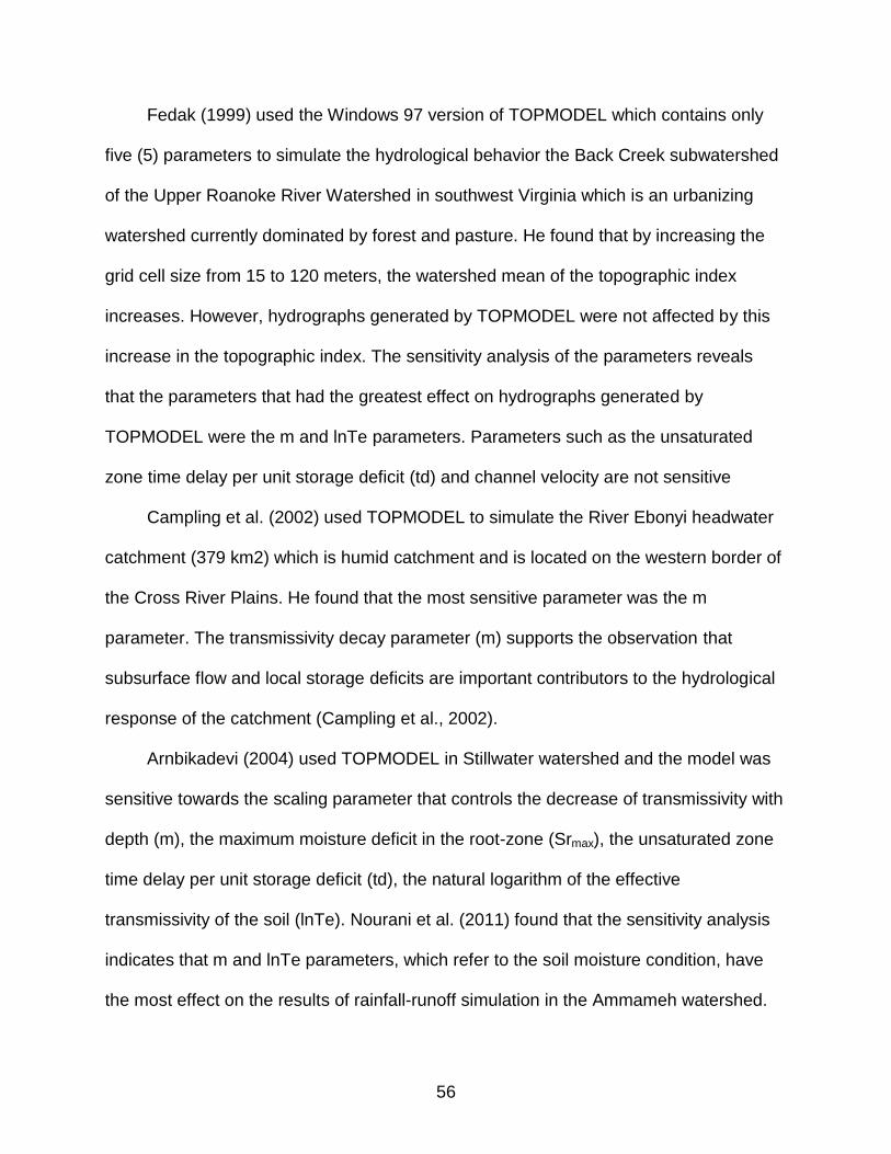
resulting in small contribution of these areas in the in Runoff at the outlet. The Figure 4-
1 shows a good relation between the topography, the topographic index and the soil
moisture.
Output of TOPMODEL
The main output generated in TOPMODEL is the streamflow. However, any
hydrological process can be simulated. Also, each version can present the output in a
different way. The easiest versions are interface interactive.
58
The R implementation of TOPMODEL does not contain all these previous options.
However, it can be coupled with GLUE which a statistical method for quantifying the
uncertainty of the model predictions
Figure 4-1. The relation between topography, topographic index ad soil moisture deficit

59
CHAPTER 5 METHODOLOGY
Sensitivity Analysis
Limitations that related to model structures, data availability on parameter values,
initial and boundary conditions will make hydrologic model application difficult.
Uncertainties that have entered the model can substantially influence the output. There
is always need to adjust model parameters for a better fit by calibration. However, the
parameter calibration process would be more efficient if it was concentrated on the
parameters that most influence the outputs of the model simulation. Also, measured
dataset is required to perform the calibration process (Wallach et al., 2006; Beven
2008).
In this study, a Local sensitivity analysis (OAT Method) and two global sensitivity
analyses (Morris Method and Fourier Amplitude Sensitivity Test Method) were
performed to understand the parameters that most influence the output of the model.
Sensitivity Analysis Process
There is a four-step general procedure for performing global sensitivity analysis
that are the determination of probability distribution functions (PDFs) of input
parameters, the generation of input samples, the computation of the computation of the
model output for each scenario and the analysis of the output distribution (Wallach et
al., 2006)
Determination of Probability Distribution Functions (PDFs) of Input Parameters
TOPMODEL uses several parameters that reflect the hydrology, soils, and location
of the catchment under investigation. Although TOPMODEL is a physically based
model, only some parameters such as ln(α/tanβ) or ln (α/T0tanβ) can be easily derived

60
from available information from the watershed characteristics. Even in the best
experimental conditions, it is always difficult to determine precisely all the required data.
Since natural systems such as soils are not homogeneous, and due to lack of
measurement, it is difficult to assign specific values to some parameters which spatially
vary in the catchment (Montesinos-Barrios and Beven, 2004; Wolock, 1993)
R-TOPMODEL is an implementation of TOPMODEL. It is based on the 1995
FORTRAN version by Keith Beven (Buytaert, 2011). Eleven parameters that are surface
hydraulic conductivity (ks), the areal average of transmissivity (lnTe), scaling parameter
(m), capillary drive (CD), initial subsurface flow (qs0), initial root zone deficit (Sr0),
maximum root zone storage deficit (SrMax), unsaturated zone time delay (td), channel
flow inside the catchment (vr) and channel flow outside the catchment (vch) are used
the R-TOPMODEL.
The selection of hydraulic conductivity technique is based on the level of
information available on physical and hydraulic properties of the soil (Maidment, 1993).
Using the soils parameters from the USDA classification, the saturated hydraulic
conductivity was calculated by the generalized Kozeny-Carman equation expressed in
the Equation (5-1).
(5-1) Where ϕe is the effective porosity, n is set equal to 4 and B equals 1058; ks has units of
cm/hr.
Calculated values obtained for the first layer (clay layer) using the Equation (5-1)
were considered as the values of the surface hydraulic conductivity. It presents a
uniform distribution between a minimum and a maximum values. The distribution of the

61
ks was expected to be lognormal. However there is no evidence that can support
lognormal distribution in the Kozeny-Carman equation (Appendix D).
The parameter lnTe [L2/T] is the log of the areal average of T0. The transmissivity
represents the integral over soil depth of hydraulic conductivity. The transmissivity is
obtained by the Equation (5-2).
(5-2)
Where k is the hydraulic conductivity, f is the scaling parameter that controls the
decrease of the hydraulic conductivity with depth and z is the thickness of each layer.
The parameter f is obtained by plotting the hydraulic conductivity of each layer.
Three values of hydraulic conductivity were obtained for each layer of the soil: a lower
value, an average value and an upper value. As indicated in Figure 5-1, three curves of
variation of the hydraulic conductivity were plotted. From these plots result three values
for the f parameter. The exponential factor governing the decrease of the hydraulic
conductivity is the f parameter.
The parameter lnTe is then obtained by taking the areal average of natural
logarithm of T0 which is the sum of the transmissivity of the layers. No particular trend of
distribution was found for T0. A maximum value and a minimum value were calculated
for the parameter. A uniform distribution was also assumed for lnTe.
The parameter m [L] is the model parameter that controls the rate of decline of
transmissivity in the soil profile. It is usually derived from an analysis of the recession’s
curves for the catchment when the assumption that the flow is derived from subsurface
drainage is made. It is usually derived from a pure recession in which recharge is

62
considered negligible. Thus, discharge has an inverse or first order hyperbolic
relationship to time. (Beven, 2001).
In this study, the scaling parameter could not be derived from recession curve.
Long-term recession was not observed for the river discharge provided by the Early
Warning Project dataset. Pure recession in which recharge can be considered being
negligible shows that the flow presents an inverse or first-order hyperbolic relationship
to time as expressed in the Equation (5-3) (Beven, 2001).
(5-3) The plot of 1/Qb should be as a straight line with slope 1/m as shown in Figure 5-2.
For the Grise River basin, even weekly recessions were difficult to be found. Few
recession curves resulting from the Early Warning Project dataset seem to provide
unrealistic values for the parameter m. From previous study (Beven et al., 1997) m
cannot obviously be extremely high as determined in the Figure 5-3 and Figure 5-3.
According to David (1993) the parameter m is calculated from the Equation (4-10).
Likewise as a function of θ a normal distribution was found for the parameter m
indicating a mean and a standard of an average ϕ is obtained for the soil by the
Equation (5-4).
(5-4)
where zi and ϕi are the thickness and the porosity of their respective layers.
SrMax [L] is computed as:
(5-5)

63
Where zroot is the root-zone depth, fc is the field capacity and is the wilting point of
the soil. The Table 3-2 presents the field capacity and wilting point based on the ASCE
classification (Rawls et al., 1983). SrMax for the entire soil was calculated by the
Equation 5-6 based on the characteristics of the soil in the Table 3-3.
(5-6)
is the difference between fc and . SrMax presents a normal distribution as a
function of θs which present normal distributions (Maidment et al., 1993).
The parameter Sr0 [L] is initial root zone storage deficit. When the gravity drainage
layer is exhausted, soil moisture will still evaporate with the rate of Ep as indicated in
the Equation 5-7. The rate of evapotranspiration loss E is assumed be proportional to a
specified potential rate Ep.
(5-7)
The initial root zone storage deficit varies in a certain range of SrMax In this study
Sr0 was kept constant. It has been demonstrated that likewise qs0, Sr0 influences the
flow process only in the beginning of model simulation. For a long simulation over 5
years of 3 hours’ time step, its influence will be insignificant.
CD [L] is the capillary drive. It is a function of the capillary suction which is the
combined adhesive forces that join the water molecules and the solid particles Morel-
Seytoux and Khanji (1974), (Bedient et al., and 2008). The capillary drive is found in the
Green Ampt infiltration method and is referred to as expressed in the Equation (5-8).
(5-8)

64
Where Ѱb is the bubbling pressure and λ is the pore-size distribution index (Parlange et
al., 1982).
According to Rawls et al. (1983), Ѱb and λ are lognormally distributed. They
provided the arithmetic and geometric mean values with the corresponding standard
deviations for both parameters, for different texture class.
Based on the parameters’ statistics obtained from Rawls et al. (1983), Hantush
and Khalin (2003) used the KINEROS2 which is event and physically based runoff and
erosion model to calculate the arithmetic means and standard deviations of capillary
drive for different soil textures by performing Monte Carlo (MC) simulations.
The Table 5-1 presents the arithmetic mean and standard deviations of the
Capillary Drive for different soil textures obtained from the lognormal approximation and
by performing 10000 Monte Carlo simulations, using the statistics of the lognormally
distributed ψb and λ (Rawls et al., 1982).
Based on the Table 5-1 provided by Hantush and Khalin for different classes of
soil, the combined capillary drive for the entire soil was calculated as stated in the
Equation 5-9.
(5-9) Where zi and CDi are the thickness and the capillary drive of their respective layers.
The channel velocity is also one of the most important parameter of R-
TOPMODEL (Parsons et al., 2004). In this study, vr [L/T] was calculated using the
Manning equation. Water level data (Stage) generated by the Early Warming Project
that has installed some instruments on the watershed was used.

65
Based on the information provided by Figure 5-5 and Figure 5-6, a rectangular
shape was adopted for the channel (Figure 5-7), where b is the bed width and y is the
stage at the measurement time. The water level gauge is installed on the bridge which
has vertical abutments, made of masonry. The Manning coefficient for natural bed is
estimated within the range 0.030- 0.035 by Chow (1959).
The location of the water level gauge was found within a range of slope of 0.8% to
1.08 % by processing the DEM in ARCGIS and the width of the bed (b) is estimated
using Google Earth at 45m. Calculated for different values of the ranges, the velocities
were then obtained as indicated in the Manning Equation as stated in the Equation (5-
10)
(5-10)
Where n is the Manning coefficient, R [L] the hydraulic radius and S is the slope of the
bed.
The velocities were plotted. A normal distribution was obtained for the velocity
since the histogram has revealed a very normal distribution for the parameter with
skewness null as showed in the Figure 5-8. The mean is 7651.56 m/h with a standard
deviation of 719.44.
The parameter qs0 [L] is initial subsurface flow per unit area. It is usually assumed
as the first measured flow. The minimum water level measured around the bridge of
Croix des Missions from August 2011 to June 2012 was 0.27m and was considered as
qs0.
The parameter td is the unsaturated zone time delay per unit storage deficit. It
controls the rate that recharge is added to the saturated zone per unit saturation deficit.

66
The parameter can be calculated as the quotient of the soil depth and the hydraulic
conductivity (Ambikadevi, 2004) as expressed in the Equation (5-11).
(5-11)
where zi and ki are the thickness and the hydraulic conductivity of their respective
layers, with i varying from 1 to 3.
The parameter dt is the time step. It corresponds to the increment in time of the
data series. The time step is 3 hours since rainfall and potential evapotranspiration data
were available t this time step.
Generation of Input Factor Samples
The local sensitivity analysis (OAT) was performed for ±10, ±20, ±50, ±100 ±150
of initial values of the parameters as presented in the Table 5-3. In some cases the
range was infeasible or unrealistic.
In the GSA, based on PDFs and the choice of SA method, the number of samples
plays an important role. R-TOPMODEL requires eleven parameters to perform.
However, all of them are not equally important for the model output. In study, some
parameters such as Initial subsurface flow per unit area (qs0), the channel flow outside
the catchment (vch), the time step (dt), the unsaturated root-zone deficit (Sr0) were
kept unchanged as indicated in the Table 5-1.
Simlab generated automatically the sampling of the parameters that were chosen
for the sensitivity analysis. Two methods which are the Morris method and the extended
FAST (Fourier Analysis Sensitivity Test) method were selected to conduct the sensitivity
analysis (SA). Parameters were chosen to be uniformly, normally or lognormally
distributed based on the literature or the calculation processes.

67
The Morris Method is well known as a screening method for environmental
models. It is an easy method that requires few simulations with easily interpretable
results (Saltelli et al., 2005). The number of simulations (N) to perform in the Morris
analysis results as indicated in the Equation (5.12).
N = r (k + 1) (5-12)
where r is the sampling size for search trajectory (r = 10 produces satisfactory results),
and k is the number of factors.
The extended FAST method uses the replicated Latin hypercube sampling to
randomly sample the k-dimensional space of the input parameters(r-LHS) design
(McKay et al., 1979; McKay 1995). The number of simulations required in this analysis
is expressed in the Equation (5.13).
N=M*k (5-13)
where m is a number between 500 and 1000. In this study M was chosen as 1000.
Computation of the Model Output for Each Scenario
Once the samples have been generated, the corresponding model output values
were computed. Codes written in R presented in the Appendix A and appendix B were
used to simulate the outputs.
Since TOPMODEL is quite simple, the running process is not really intensive. A
few minutes were enough for the simulation. The ouput values generated from this
process were formatted for the analysis in Simlab wich was used for the global
sensitivity analysis.

68
Analysis of the Output Distribution
For the OAT method, the analyses were carried out for specific values such as
minimum, median, maximum and total streamflow. A slope was constructed between for
the variation of the values. The bigger slope indicates the greater change.
For the Global Sensitivity analyses, outputs obtained from the model runs were
stored in the desired SimLab post-processing format to run the statistical analysis that
generates sensitivity indices and parameter rankings. SimLab analyzed the data and
calculate sensitivity indexes of the Morris and the extended FAST methods.
In the Morris Method, the characterization the distribution of Fi through its mean μ
and standard deviation (ᵟ) presents meaningful information about the of ith factor on the
output. A factor with a high mean presents a significant overall influence on the output;
a high standard deviation indicates either a factor interacting with other factors or factor
whose effect is nonlinear (Saltelli, et al., 2004).
In the FAST Method, the expected value and the variance of the output are
estimated. The contribution of individual factor to the variance of the output is also
estimated (Cukier et al., 1973). Two types of indices are generated: the first order
indices (Classical FAST) which measure the main effect of factors. The second ones
are the Total Sensitivity Indices (TSI) in the Extended FAST. The TSI of a parameter is
the sum of all the sensitivity indices involving this parameter. They compute the total
effect of the factors. The extended Fast analysis adds up the impacts of each factor and
their interactions with other factors. Usually, When the TSI is greater than 0.8 the
parameter is considered as very important; between 0.5 and 0.8 it is said to be
important; when it is between 0.5 and 0.3 the parameter is not important; below 0.3 the
parameter is said to be irrelevant (Sobol et al., 1990a, 1990b, 1993, Chan et al., 1997).

69
Excel was used to construct the output probability distributions such as Cumulative
Distribution Frequency (CDF) and histograms.
Data Elevation Model (DEM)
The DEM is one of the most important data used by TOPMDEL. The DEM used in
this study was obtained from the Advanced Spaceborne Thermal Emission and
Reflection Radiometer (ASTER) Global Digital Elevation Model (GDEM). Land surfaces
between 83°N and 83°S are encompassed by the ASTER GDEM. It is composed of
22,600 1°-by-1° tiles. Tiles that contain at least 0.01% land area are included. The
ASTER GDEM is in GeoTIFF format with geographic latitude and longitude coordinates
and a 1 arc-second (30 m) grid of elevation postings. It is referenced to the
WGS84/EGM96 geoid. Estimated accuracies for this global product were 20 meters at
95 % confidence for vertical data and 30 meters at 95 % confidence for horizontal data
before the production.
Topographic Index
The obtained DEM was processed using ArcGIS 10 (Arc Map 10) to delineate the
Grise River watershed. After the extraction of the watershed using watershed
delineation tools available in the (Arc Map 10), the output raster format is transformed
into a text file format (ASCII) which can be used by the R-TOPMODEL version. Pixels
outside the catchment area are given a distinct value that is set to NA in R. The -9999
value was set as the NA. The DEM was imported as a matrix which can then be
processed by the topidx () function in R-TOPMODEL to obtain the Topographic index
required by TOPMODEL.

70
Data
Data used to conduct the research was downloaded from the North American
Regional Reanalysis (NARR) model. The NARR model is produced by the National
Centers for Environmental Prediction (NCEP) and takes in, or assimilates a great
amount of observational data to produce a long-term picture of weather over North
America. A Matlab code (see Appendix A) was written to download 3-hrs precipitation
and potential evapotranspiration over 1998 to 2002.
However, in comparison to monthly and annual totals available in the literature,
NARR has overestimated the rainfall and potential evapotranspiration. To correct the
data, monthly values are calculated for the NARR dataset. The dataset was compared
to FAO monthly data. NARR data was also twice the average available in the literature.
A factor of correction was calculated and applied to the NARR dataset. This factor was
0.55.
Soil information in this study is provided by Harmonized World Soil Database
(HWSD) which is an initiative of Food and Agriculture Organization of the United
Nations (FAO) and the International Institute for Applied Systems Analysis (IIASA) to
combine recently collected data of soil information with the information already
contained within the FAO-UNESCO Digital Soil Map of the World.
Model Run
The version of TOPMODEL used to perform the hydrological simulation of the
River Grise basin is the 97 version built in R. This implementation of TOPMODEL was
performed by Buytaert et al., (2005). Codes written in R (see appendix A and B)
provided in this package were modified to perform the processes encompassed in this

71
research. For the global sensitivity analysis, sampling are generated as stated before
using SimLab
Table 5-1. Summary statistics of CD (cm) parameter for various soil types
Soil texture
Arithmetic Geometric
Mean Std MC
theo. MC theo. MC Mean Std
Sand 39 40 118 156 9.9 5.3 Loamy sand 41 44 131 156 12.3 4.8 Sandy Loam 64 62 186 153 22.1 4.3 Loam 105 112 475 493 17.9 6.9 Silt loam 158 156 563 544 33.5 5.8
Sandy clay loam 181 180 864 800 44.
1 5 Clay loam 129 129 364 309 42.3 4.5 Silty clay loam 195 183 601 561 55 4.9 Sandy clay 219 224 909 937 48.6 5.9 Silty clay 209 204 666 583 59 4.9 Clay 242 232 770 689 64.1 5
From: Mohamed M. Hantush and Latif Kalin (2003) Std: standard deviation theo: theorical MC: Monte Carlo

72
Table 5-2. TOPMODEL parameters and their values for GSA
Min: Minimum value Max: Maximum value Stdev: Standard deviation *This parameter is not really used in TOPMODEL
Parameters values for Simulation and Global sensitivity analysis
Parameters
Min Initial / mean
Max Stdev Distribution
qs0 : Initial subsurface flow per unit area [m] 0.27 constant LnTe :log of the areal average of T0 [m2/h] -1.85 -0.61 0.35 uniform
m : Model parameter [m] 0.450 0.13 normal
Sr0 : Initial root zone storage deficit [m] 0.01 Constant SrMax : Maximum root zone storage deficit [m] .449 0.13 normal td : Unsaturated zone time delay per unit storage deficit [h/m]
0.43 3 4.80 uniform
vch* : channel flow outside the catchment [m/h] 4500 constant
vr : channel flow inside catchment [m/h] 7651.56 719.44 normal
k0: Surface hydraulic conductivity [m/h] 0.055 0.667 uniform CD : capillary drive, see Morel-Seytoux and Khanji (1974) [m]
0.48 0.048 lognormal
dt : The time step [hours] 3 Constant

73
Table 5-3. TOPMODEL parameters and their values for LSA
Parameters values for Simulation and Local sensitivity analysis
Parameters -300% -200% -100% -50% -20% -10% Initial 10% 20% 50% 100% 200% 300%
qs0 [m] 0.27 0.27 0.27 0.27 0.27 0.27 0.27 0.27 0.27 0.27 0.27 0.27 0.27
LnTe [m2/h] 1.22 0.61 0 -0.305 -0.488 -0.549 -0.61 -0.671 -0.732 -0.915 -1.22 -1.83 -2.44
m [m] - - - 0.225 0.36 0.405 0.45 0.495 0.54 0.675 0.9 1.35 1.8
Sr0 [m] 0.01 0.01 0.01 0.01 0.01 0.01 0.01 0.01 0.01 0.01 0.01 0.01 0.01
SrMax [m] - - 0 0.2245 0.3592 0.4041 0.449 0.4939 0.5388 0.6735 0.898 1.347 1.796
td [h/m] - - 0 1.5 2.4 2.7 3 3.3 3.6 4.5 6 9 12
vch [m/h] 4500 4500 4500 4500 4500 4500 4500 4500 4500 4500 4500 4500 4500
vr [m/h] - - - 3825.8 6121.2 6886.4 7651.6 8416.7 9181.9 11477 15303 22955 30606
k0 [m/h] - - 0 0.25 0.4 0.45 0.5 0.55 0.6 0.75 1 1.5 2
CD[m] - - 0 0.24 0.384 0.432 0.48 0.528 0.576 0.72 0.96 1.44 1.92
dt [h] 3 3 3 3 3 3 3 3 3 3 3 3 3
Spaces mark “-“ are unrealistic or unfeasible values

74
Figure 5-1. Decrease of the hydraulic conductivity with average depth

75
Figure 5-2. Derivation of an estimate of parameter m using recession curve analysis under exponential transmissivity profile assumption (Beven, 2001)
Figure 5-3. Recession curve for the third week of December, 2011

76
Figure 5-4. Recession curve for the first two weeks of January, 2012
Figure 5-5. Bridge of Croix des Missions in dry seasons

77
Figure 5-6. Bridge of Croix des Missions in rainy seasons
Figure 5-7. Shape of the channel at the stages gauge

78
Figure 5-8. Distribution of the channel velocity inside the catchment

79
CHAPTER 6 RESULTS AND DISCUSSIONS
Model Justification for the Watershed
The climate of the watershed where TOPMODEL is being applied varies whether it
is the lowland or the mountain. In the lowland, the rainfall varies form 1300 mm to
around 1000mm. while the climate is rather humid in the upstream with the annual
rainfall varying from 1450 mm in Petionville to 2000 mm in Kenscoff. The depth to water
is usually between 5 and 50 m. In the mountains, depth to water is usually higher than
100 m. Seasonal fluctuation in the water levels can be great (Knowles et al., 1999).
Also Haiti is a data-sparse region. Too demanding model in parameter cannot be
applied there since it is difficult to find necessary data for parameters calculation.
As a result, the topographic and climate conditions of the watershed are not
necessarily the best but are more or less suitable for the application of TOPMODEL.
Also, since TOPMODEL does not require too many parameters compared to usual
hydrological models, it was a convenient choice to use TOPMODEL.
DEM of the Catchment
The Figure 6.1 a represents the DEM of the River Grise catchment resulted from
ArcGIS processing. This processed DEM was used in the R-TOPMODEL package to
derive the Topographic Index. However, only the upstream part of this DEM contributes
as drainage area.
The Figure 6-2 represents the hydrological cumulative area map. Located in the
upper part of the watershed, only this area seems to contribute water based on the
direction of the flow computed using the DEM. While the real watershed area is 393km2,
approximately only 290 km2 was able to be processed by R-TOPMODEL using the

80
DEM. The determined outlet is different from the natural outlet observed on the real
catchment.
However, it is important to notify that the flow computational process of this R-
TOPMODEL version is based on multiple and single flow which is different from the
algorithm used in ArcGIS. We also know that the lower part of this catchment is a flat
area.
Topographic Index Results
The Figure 6-3 presents the areal distribution of the Topographic Index in the
River Grise watershed. The areal average of the topographic index is 12.588 with the
highest Topographic Index approximately 22. However, 93 percent of the surface of the
catchment delineated by TOPMODEL has a topographic index lower than the average.
As presented in the Figure 4-1, the soil moisture deficit index in inversely proportional to
the topographic index. Since the soil moisture deficit indicates when runoff starts for
each grid cell, locations with low topographic index are more likely to generate runoff.
The areal distribution of the topographic index reveals that the topographic index is
lognormally distributed and skewed to the right in this catchment. More than 80 % of the
watershed has a topographic index lower than 8. This catchment varies in altitude from
approximately 50m to 2000m and presents steep slopes which indicate that this soil can
easily become dry. However, due to steep slopes that prevail in this catchment surface
runoff can be very important. Depressions can be almost inexistent to stock water while
infiltration can be expected to be low.

81
Sensitivity Analysis
The following paragraphs present the sensitivity analysis results. The sensitivity
analyses were realized for the 5 years of data. Both LSA (OAT) and GSA (Morris and
FAST methods) results are presented below.
Local Sensitivity Analysis (OAT)
Model sensitivity was performed for ±10, ±20, ±25, ±50, ±75 ±100 ±150 of initial
values of the parameters as presented in the Table 5-3. Model sensitivity is reported as
the percent difference of model results as compared to the base simulation.
The Figure 6-4 presents the influence of the parameters on the minimum flows as
depicted by the Local Sensitivity Analysis (LSA). The parameter m presents the most
important influence. The parameters lnTe, SrMax and Ks are also showed important. The
slope showed by the parameters indicates their level of influence on the output. The
parameter m presents the largest slope within the range of variation, which is within the
range obtained from the calculations. Also, the increase of the parameter m increases
the mimimum flows. However the increases of the SrMax and lnTe decrease the
minimum flows.
Local Sensitivity Analysis (LSA) for the median flows is showed on the Figure 6-5.
Within the range calculated from the watershed characteristics, the parameter SrMax is
the most important since its slope is larger for the range of distribution of the
parameters. When the parameters SrMax and m increase, the median flows decrease.
The Figure 6-6 presents the influence of the parameters on the average flows. The
parameter SrMax presents the most important influence for the range of variation
considered for the calculations of the parameters. Its slope is the steepest. Other
parameters such as hydraulic conductivity (ks) and the decay factor the decrease of the

82
transmissivity with depth (m) are also important as showed on the Figure 6-6. Average
runoff decreases also with the increase of the soil moisture defict. The same trend is
observed for the parameters m and ks.
The Figure 6-7 presents the influence of the parameters on the maximum flows as
depicted by the Local Sensitivity Analysis (LSA). The channel velocity is clearly the
most important parameter influencing the runoff. It remains dominant in all range of
variation. Maximum runoff increases with the increase of the channel velocity until it
becomes stable.
The Figure 6-8 presents the influence of the parameters on the Total flows for the
Local Sensitivity Analysis (LSA). Likewise for the average flows, SrMax presents the most
important influence for the common range of variation considered for the calculations of
the parameters.
The LSA method reveal that the most important parameters are the transmissivity
(lnTe), the scaling parameter of the decline of transmissivity (m), Maximum root zone
storage deficit (SrMax) the hydraulic conductivity (ks) the channel velocity inside the
catchment (vr) . Their sensitivity varies wih the type of flows.
The scaling parameter of the decline of transmissivity (m), Maximum root zone
storage deficit (SrMax) the hydraulic conductivity (ks) seem to have a constant influence
on almost all type of the flow output whether it is low or high flow.
Global Sensitivity Analysis
The following paragraphs present the Morris and the FAST sensitivity analyses.
Due to the similarity between the results of the analyses for average flows and total
flows, only the analyses for the total flows are presented.

83
Morris sensitivity analysis
The relative importance of the TOPMODEL parameters on the output based on
the Morris Method is presented in the Table 6-1. Eighty (80) hydrographs were
generated for the Sensitivity Analysis. Minimum, Maximum, Mean, Median and Total
were calculated and were used for the sensitivity analysis.
The graphs 6-9 to 6-13 plot the indexes of sensitivity of each parameter on the
minimum, maximum, mean, median, and the total flows. μ* represents the total
influence of the factor which the sum of the primary and the interactions while the
standard deviation (ᵟ) represents the interactions themselves. While presenting more
information showing the impact of interactions within the parameters, the Morris method
confirms the results revealed by the OAT analysis.
The Figure 6-9 plots the Global sensitivity analysis results or the minimum flows
obtained from the Morris screening method. As indicated on the graph, the areal
logarithm of transmissivity (lnTe), the decay factor (m), the moisture deficit (SrMax), and
the hydraulic conductivity (ks) are the most sensitive parameters for the minimum flows.
However, the transmissivity decay seems to affect the most the minimum flows followed
by the transmissivity. Not only are they important by their total influence but also they
primarily impact since they are located below the angle 45 degree (Morris, 1991).
Hydraulic conductivity and the moisture deficit seem to have a greater contribution
through interactions. While the impact of the channel velocity and the unsaturated zone
time delay being null on the minimum flows, the capillary drive seems to have a small
impact with equal primary and interactions contributions.

84
The impact of the parameters on the median (Q0.50) flows is presented on the
Figure 6-10. The parameters such as the areal logarithm of transmissivity (lnTe), the
decay factor (m), the moisture deficit (SrMax), the hydraulic conductivity (ks) and the
channel velocity are the ones that influence the output. However, the soil moisture
deficit parameter has the greatest influence according to the results obtained from the
Morris screening method. The hydraulic conductivity and areal logarithm of the
transmissivity seem contribute equally by the primary and their interactions whereas the
deficit moisture has a higher influence through his primary effect while the channel
velocity presents higher influence by interactions. Parameters such as Capillary Drive
and unsaturated zone time delay for per unit storage deficit don’t influence the output.
The Figure 6-11 presents the GSA results for the averagel flows obtained by the
Morris method. Three (3) parameters that are the soil moisture deficit (SrMax), the decay
factor of the transmissivity with depth (m) and the hydraulic conductivity (ks) show
important effect on the flows. The moisture deficit presents the greatest influence. It also
has the greatest primary effect. The scaling parameter for the decline of the
transmissivity in the soil seems to contribute equally by interactions and by its primary
impact.It seems to be located on the bisectrix of the origin angle. The hydraulic
conductivity seems to contribute more by its interactions. The other parameters present
no effect on the average flows.
The Figure 6-12 plots the Global sensitivity analysis results the maximum flows
obtained from the Morris screening method. All the parameters but the unsaturated
zone time delay per unit storage deficit seem to be detached from the origin, and
consequently have an influence on the output. The channel velocity presents a more

85
important influence on the maximum flows whereas the other parameters seem to have
small influence. It is also remarkable that all they parameters have a greater primary
effect but the channel velocity that seems to contribute equally by its primary effect and
by its interactions.
As indicated on the Figure 6-13 that presents the Global sensitivity analysis results
or the Total flows obtained from the Morris screening method, only three parameters
have an important effect on the total flows: the moisture deficit which presents the
greater influence has also a greater primary effect, the scaling parameter for the decline
of the transmissivity in the soil seems to contributes equally by interactions and by its
primary impact, and the hydraulic conductivity that contributes more by its interactions.
The pattern showed by the Total flow is the same as the one observed for the average
flows Parameters such as the logarithm of the areal transmissivity, the Capillary Drive,
the channel velocity, and the unsaturated zone time delay for storage deficit present no
effect on the total flows.
The plots of the Screening Method results of the sensitivity indexes of the
parameters reveal the parameters are not all neither equally sensitive. Only five (5) of
them such as the transmissivity (lnTe), the scaling parameter of the decline of
transmissivity (m), Maximum root zone storage deficit (SrMax) the hydraulic conductivity
(ks) the channel velocity inside the catchment (vr) seem to influence the runoff
simulation of R-TOPMODEL. Also their influence seems to vary whether the flows are
low or high.
The Morris analysis reveals that the scaling parameter of the decline of
transmissivity (m), Maximum root zone storage deficit (SrMax) the hydraulic conductivity

86
(ks) seem to constantly influence the flow output whether it is low or high flow. This is
illustrated in the Figures 6-9 to 6-13.
However, the channel velocity inside the catchment (vr) seems to have significant
influence on the median (Q0.50) and the maximum flows. Parameters such as
unsaturated zone time delay per unit storage deficit (td) and capillary drive (CD) seem
to have no influence on the output.
FAST sensitivity analysis
The process used for the Morris Method was duplicated for the FAST Method
analysis. The relative importance of the TOPMODEL parameters on the output based
on the FAST Method is presented in the Table 6-2 and Table 6-3. Seven thousands
(7000) simulations were generated for the Sensitivity Analysis. Minimum, maximum,
mean and median and total hydrographs were calculated and were used for the
sensitivity analysis.
Two categories of plots are presented. First, the sensitivity indexes of the first
order which indicate the impacts of the parameters without interactions; Second, the
level of influence of the parameters through interactions. The interactions are obtained
by subtracting the first order indices from the total order indices. The analyses were
performed using the minimum, median, mean, maximum, and total flows.
The Figure 6-14, Figure 6-15 and Figure 6-16 plot the Global sensitivity Test
results obtained from the Fourier Amplitude Sensitivity Test method. According to the
plots the scaling parameter for the transmissivity (m) the areal logarithm of
transmissivity (lnTe), the maximum storage deficit (SrMax), and the hydraulic conductivity
(ks) are the most sensitive parameters for the minimum flows. However, the scaling
parameter of the transmissivity affects the most the minimum flows and remains the

87
important one based on the Sobol’s classification (Sobol et al., 1993), since it is the only
one to present a total index higher than 0.5 (Figure 6-14). As indicated by the Figure 6-
15, the primary effects of the parameters such as channel velocity, the capillary drive
and the unsaturated zone time delay of the storage deficit are null. It is also noticeable
that interactions have low impacts on the minimum flows as confirmed by the Figure 6-
16.
The impacts of the parameters on the median (Q0.50) flows are presented on the
Figure 6-14 and Figure 6-15. According to the Figure 6-14 the maximum storage deficit
(SrMax) controls the median flows. While SrMax is responsible for approximately 65% all
the remaining parameters show indexes lower than 5%. All the parameters seem to
influence the median flows (Q0.50) laying within the range of 10% to 20%. However,
according to the Sobol’s classification, only SrMax is very important while the others are
irrelevant.
Based on the GSA results obtained from the FAST method depicted on the Figure
6-14 the maximum moisture deficit parameter is the most important factor influencing
primarily the average flows. It is responsible for approximately 85% followed
insignificantly by the scaling parameter for the decline of the transmissivity with depth
(m), and the hydraulic conductivity (ks) that are responsible for less than 10%. Also, the
interaction effects are very low on the average flows; as a result some parameters such
as the unsaturated zone time delay for moisture deficit (td), the channel velocity (vr) and
capillary drive (CD) appear to be negligible. Likewise the OAT and the Morris analyses,
The FAST analysis of the average flows presents the same pattern as the total flows

88
The Global Sensitivity Analysis obtained from the FAST method for the first order
indexes shows that only the channel velocity has a very significant impact on the
maximum flows as presented that the Figure 6-15. It is responsible for 40%; all the other
parameters appear to be negligible. However, the Figure 6-16 which presents the FAST
results of the interactions seems to show that all the parameters have significant
influence on the maximum flows in the River Grise watershed. They vary from 30% to
50%.
However based on the Sobol’s classification related in Chapter 5, only parameters
with total sensitivity index (TSI) higher than 0.3 would be considered as important. In
this case, only three (3) parameters would remain important that are the decay
parameter for the transmissivity decrease with depth (m), the soil moisture deficit (SrMax)
and the channel velocity (vr) would be important for this study.
The Fourier Amplitude Sensitivity Test method used for the sensitivity analysis
strengthens and quantifies the results revealed by the Morris method. The sensitivity
varies with the parameters and with low and high flows. The transmissivity (lnTe), the
scaling parameter of the decline of transmissivity (m), maximum root zone storage
deficit (SrMax), the hydraulic conductivity (ks) and the channel velocity inside the
catchment (vr) are the parameters that have influenced the hydrologic response of the
catchment. The scaling parameter of the decline of transmissivity (m), maximum root
zone storage deficit (SrMax), and the hydraulic conductivity (ks) seem to remain
constantly the most sensitive. However, only important m, vr and SrMax appear to be
important or very important based on the type of flows while the other parameters are
whether not important or irrelevant based on the type of flows.

89
Parameters such as the unsaturated zone time delay per unit storage deficit (td)
and capillary drive (CD) seem to be present more through interactions.
Discussions of the Parameters Impacts
The m parameter
The m parameter is the model parameter that controls the rate of decline of
transmissivity in the soil profile (Beven, 1984). The simulation of the River Grise basin
by TOPMODEL reveals that the m parameter is very sensitive for both Global and Local
Sensitivity Analyses. It appears to be the most sensitive for the minimum flows with
which it varies proportionally. According to the Figure 6-4, in the range of variation of the
decay parameter of the transmissivity with soil depth (m) for the watershed as
presented in the Table 5-2, when the parameter increases the minimum flows increases
and vice versa. However the parameter m is inversely to the other flows. When it
decreases the average flows, the median flows, the maximum flows and the total
increase and vice versa.
As a parameter related to recession flow in the watershed, it seems to be
reasonable that m be the most important parameter for minimum flows. It can be
assumed that the methodology used for the calculation of the parameter is consistent
with the nature of the parameters itself.
In term of management actions, the parameter m can help in predicting the water
lost by the aquifer or even expected in the downstream for others activities. In dry
seasons, the river is alimented by the groundwater that consequently decreases. The
recession curve can tell about the volume stored at any given time. Indeed, if m is
determined for a specific watershed, it is possible to evaluate its storage capacity by
integration over the time interval. The determination of the water available in recession

90
time is important to evaluate the amount of water to provide in support to the low flow in
dry seasons.
The lnTe parameter
The lnTe parameter is the natural logarithm of the effective transmissivity of the
soil at saturation [m2/h]. This parameter is also an important parameter as indicated by
both sensitivity analysis methods. It appears to be more sensitive for the minimum flows
likewise its scaling parameter m. It does not seem to be very sensitive for any other type
of flows. It varies proportionally with the minimum flows. When it decreases the flows
decrease and vice versa. However, likewise m, its variation is inversely proportional to
the other flows. When the natural logarithm of the effective transmissivity of the soil at
saturation decreases these flows increase and vice versa.
Likewise the parameter m, it is related to the recession (minimum flows) in the
watershed. The transmissivity of the soil can tell about the ability of the soils in the
watershed to stock water in rainy seasons and to release it during the dry seasons.
The SrMax parameter
The SrMax parameter is the maximum root zone storage deficit parameter in
TOPMODEL. It controls the moisture deficit in the soil. It is the most sensitive parameter
of TOPMODEL as revealed in this study. It appears to be important whether for
minimum, average or high flows. As a continuous model, TOPMODEL accounts for the
amount of moisture in the soil between rainfall events. According to the stage dataset,
the watershed seems not to suffer from long term drought. Also, by nature, the moisture
deficit is built to reflect any moisture situation in the watershed. It is more likely to be
sensitive to any types of flows.

91
It is important to notice that the soil moisture deficit is inversely proportional with all
types of flows. When the moisture deficit increases the flows decreases and vice versa.
This is very important in term of management actions. By increasing the capacity of the
soil to stock more water the amount of water to be released on rainfall event will
necessarily decrease. The importance of vegetation in increasing the porosity of the soil
is well known. Therefore a reforestation campaign can be a good action against flood
occurrence in the watershed.
The ks parameter
The ks parameter is the surface hydraulic conductivity at saturation [m/h]. This
parameter is also an important parameter as indicated by both sensitivity analysis
methods. It is one the most widely sensitive parameters. It appears to be sensitive for all
types of flows. It is well know that the hydraulic conductivity is very important parameter
for the runoff generation in every hydrologic model since it describes the ease with
which water moves through pore spaces.
The hydraulic conductivity presents a proportional relationship with the minimum
flows for values between 0.25 and 1 m/h before starting to present no significant
increase of the minimum flows. The relationship seems to level off after the hydraulic
conductivity reaches 1m/h. It also seems to present a proportional relationship with the
maximum flows but it is not significant. However the relationship seems to be inversely
proportional to the other flows.
The hydraulic conductivity is Hydraulic conductivity is a property of the porous
media. It depends on the pore size, its distribution, and its connectivity. Vegetation can
help in fracturing the soil to create more pores. When the porosity of the soil increases
the hydraulic conductivity will also increase.

92
The vr parameter
The vr parameter is the channel flow inside catchment [m/h]. The simulation of the
River Grise basin by TOPMODEL reveals that the channel velocity is also sensitive for
both Global and Local Sensitivity Analyses. It appears to be the most sensitive for the
maximum flows. It does not seem to be too sensitive for other types of flows but
maximum and median flows. This is the parameter of the effective surface routing
velocity for the distance/area procedure. As linear routing is assumed in TOPMODEL, it
is comprehensible that the parameter is more important for high flows.
The channel velocity presents proportional variation with the maximum flow. The
other types of flows don’t show any significant variation with the variation of the channel
velocity.
The parameters td and CD
The parameters td [h/m] and CD [m] that represent respectively the unsaturated
zone time delay for root zone deficit and the capillary drive happen not to be really
sensitive in the simulation of the River Grise catchment. They seem to have no primary
effect on any flows. Their contributions appear only through interactions with other
parameters. The situation of these parameters in this study happens not to be different
from what that has been found in the literature.
Theseparameters did not show any significant variation with any type of flows.
Indeed this was expeted because these parameters remain non important in these
study and are usually revealed to be non important in the literature related to
TOPMODEL application studies.

93
Discussions of the Sensitivity Analysis Results
The results obtained the three analysis methods seems not to be significantly
different. They are even more similar for some specific output such as the minimum
flows, the average flows and the total flows.
It seems that the interactions which are taken into account in the global sensitivity
analysis (GSA) and neglected in the local sensitivity analysis (LSA) are really not
important for almost all the outputs. When the interactions are important for the
maximum flows for example, the parameters that have the most important primary
effects are also the ones that have the most important interaction effects. As a result,
their total sensitivity index remains the most important for both GSAand LSA methods.
FAST Uncertainties
Likewise the sensitivity analysis, simulation results provided by some selected
outputs of the FAST analysis have been used to carry out uncertainty analyses. The
uncertainty analysis determines the ranges of variation of the flows whithin the
watershed. Analyses have been carried out for Minimum, Median, Mean, Maximum and
Total and are presented on the Figures 6-17 to 6-21. Table 6-4 presents the uncertainty
analysis statistics for the probability distributions of the selected results.
As indicated in the Table 6-4, the 95% confidence interval for the minimum flows
lays within the 0.002 - 0.006 m3/3h. With an average flow of 0.004m3/3h, its cumulative
distribution frequency, represented by the Figure 6-17, reveals that almost 95% of the
flows are lower than 0.01m3/3h.
The median flows vary from 0.011 m3/3hto 0.253 m3/3h. The statistics are
presented in the Table 6-4.The 95 % confidence interval goes from 0.049 to 0.148

94
m3/3h with an average of 0.103 m3/3h. Approximately 85% of the flows are lower than
0.13 m3/3h as presented in the Figure 6-18.
The average flows vary from 0.333 m3/3h to 0.467 m3/3h with an average of 0.390
m3/3h.The 95 % confidence interval lays within 0.357 m3/3h -0.427 m3/3h (Table 6-
4).The distribution of frequency of the flows presents a normal distribution shape.
However, the cumulative distribution frequency (CDF) reveals that more than 85 % of
the flows is lower than 0.41 m3/3h.The average itself (0.389 m3/3h) is higher than more
than 80 % of flows as indicated in the Figure 6-19.
The maximum flows represented by the Figure 6-20 present a very particular
shape compare to rest of the flows. The 95% confidence interval varies within 6.403
m3/3h and 6.554 m3/3h. The range of variability is goes from 6.107 m3/3h to 6.569
m3/3h with an average of 6.538m3/3h. The distribution of the frequency is very much
skewed to the left. Most of the distribution of frequency represents approximately 10 %
of the cumulative distribution function. The distribution seems to be lognormal as
showed in the Figure 6-20.
The total for the 5 years under analysis presents a very normal distribution of the
flows. The statistics are presented in the Table 6-4 and the Figure 6-21 presents the
cumulative distribution of frequency and the density of the distribution. The flow range
varies between 4866.803 m3/3h and 6810.111 m3/3h.The average flow is
5689.584m3/3h which is not very different from the median flow. The 95 % confidence
interval goes from 5208.013 m3/3h to 6817.795 m3/3h. Approximately 90% of the flow is
cumulative distribution of the frequency curve (CDF) is lower than 5,966.44 m3/3h.

95
Table 6-1. Three (3) hours sensitivity Indexes for the Morris Analysis
QMinimum Q050 QMean QMaximum QTotal Morris Index
Mu
Sigma
Mu
Sigma
Mu
Sigma
Mu
Sigma
Mu
Sigma
lnTe 0.0023 0.0011 0.0032 0.0025 0.00052 0.000559 0.0073 0.0055 8.0429 8.262
m 0.0026 0.000846 0.0151 0.006 0.0135 0.0037 0.0074 0.0043 197.1407 54.4739
SrMax 0.0009 0.00093 0.0546 0.019 0.0507 0.0063 0.0044 0.0047 741.2635 91.6451
td 0 0 0.00008 0.00014 0.00002 6.32E-05 0.0004 0.000843 0.4047 0.9028
Vr 0 0 0.0228 0.0243 0 0 0.0202 0.0338 0.2154 0.0306
ks 0.0008 0.0009 0.0103 0.0088 0.0106 0.0082 0.0075 0.006 155.0077 119.45
CD 0.0001 0.0001 0.0008 0.0007 0.0008 0.0004 0.0019 0.0027 11.575 6.5966
Mu: Mean Sigma: Standard deviation QMinimum: Minimum flows QMean: Average flows Q050: Median flows QMaximum: Maximum flows QTotal: Total flows

96
Table 6-2. Three (3) hours sensitivity Indexes for the FAST First-Order Analysis
FAST First-Order indexes
Parameters QMinimum Q050 QMean QMaximum QTotal
LnTe 0.2528 0.0022 7.61E-05 0.000363 7.45E-05
M 0.4748 0.0331 0.0587 0.000728 0.0587
SrMax 0.0833 0.6545 0.8474 0.0018 0.8474
Td 3.41E-05 5.98E-05 4.25E-05 0.000198 4.24E-05
Vr 9.66E-06 0.03 4.38E-05 0.4076 4.35E-05
K0 0.0578 0.0213 0.0311 0.0029 0.0311
CD 0.000317 0.000433 0.000445 0.000223 0.000444
QMinimum: Minimum flows QMean: Average flows Q050: Median flows QMaximum: Maximum flows QTotal: Total flows

97
Table 6-3. Three (3) hours sensitivity Indexes for the FAST Total-Order Analysis
QMinimum: Minimum flows QMean: Average flows Q050: Median flows QMaximum: Maximum flows QTotal: Total flows
FAST Total-Order Indexes
Parameters QMinimum Q050 QMean QMaximum QTotal
LnTe 0.313557 0.116777 0.019069 0.311441 0.01905
m 0.53126 0.173188 0.078369 0.316737 0.078375
SrMax 0.12617 0.844516 0.911686 0.309478 0.911699
td 0.010351 0.120499 0.026736 0.299767 0.0267
vr 0.012245 0.221672 0.02812 0.920816 0.028131
K0 0.09388 0.179756 0.056358 0.43335 0.056325
CD 0.016355 0.16329 0.030488 0.424807 0.030478

98
Table 6-4.Uncertainty analysis statistics for probability distributions obtained from the FAST results
Range Mean Min Q2 95 %CI Max Kurtosis Skew Standard Deviation
Qminimum 0.008 0.004 0.000 0.004 0.002-0.006 0.008 0.236 0.280 0.001
Q0025 0.015 0.007 0.001 0.006 0.003-0.011 0.015 -0.194 0.532 0.002
Q025 0.024 0.011 0.003 0.010 0.005-0.020 0.027 -0.589 0.550 0.004
Q050 0.242 0.103 0.011 0.105 0.049-0.148 0.253 1.300 -0.064 0.025
Qmean 0.134 0.390 0.333 0.389 0.357-0.427 0.467 0.407 0.291 0.018
Q075 0.331 0.616 0.468 0.618 0.523-0.710 0.799 -0.236 -0.015 0.049
Q0975 0.353 1.836 1.650 1.832 1.754-1.932 2.003 0.133 0.201 0.046
Qmaximum 0.462 6.538 6.107 6.548 6.403-6.554 6.569 33.322 -5.401 0.041
Qtotal 1951 5690 4867 5678.6 5209.6-6236.5 6817.8 0.407 0.291 261.405
Range: Difference between Maximum flows and Minimum flows Min: Minimum flows Q2: Flows for 0.50 percentile Mean: Average flows Max: Maximum flows Qtotal: Total flows

99
Figure 6-1. DEM of the River Grise catchment

100
Figure 6-2. Map of the area processed by R-TOPMODEL
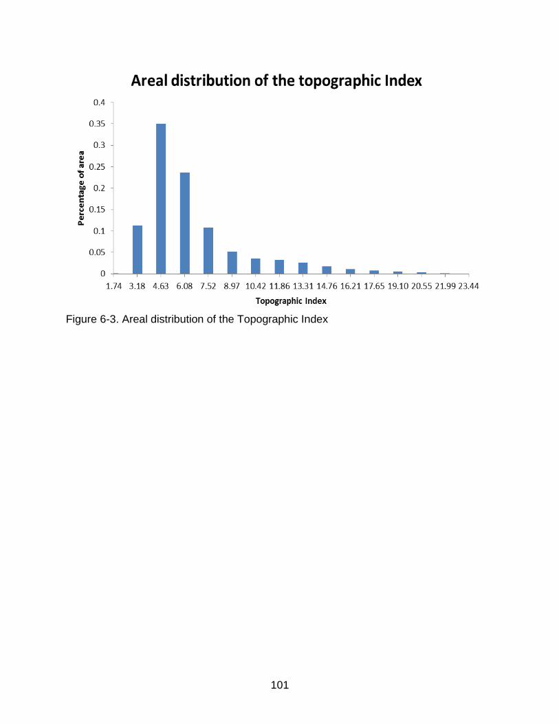
101
Figure 6-3. Areal distribution of the Topographic Index

102
Figure 6-4. OAT sensitivity of the parameters for the minimum flows
Figure 6-5. OAT sensitivity of the parameters for the Median flows
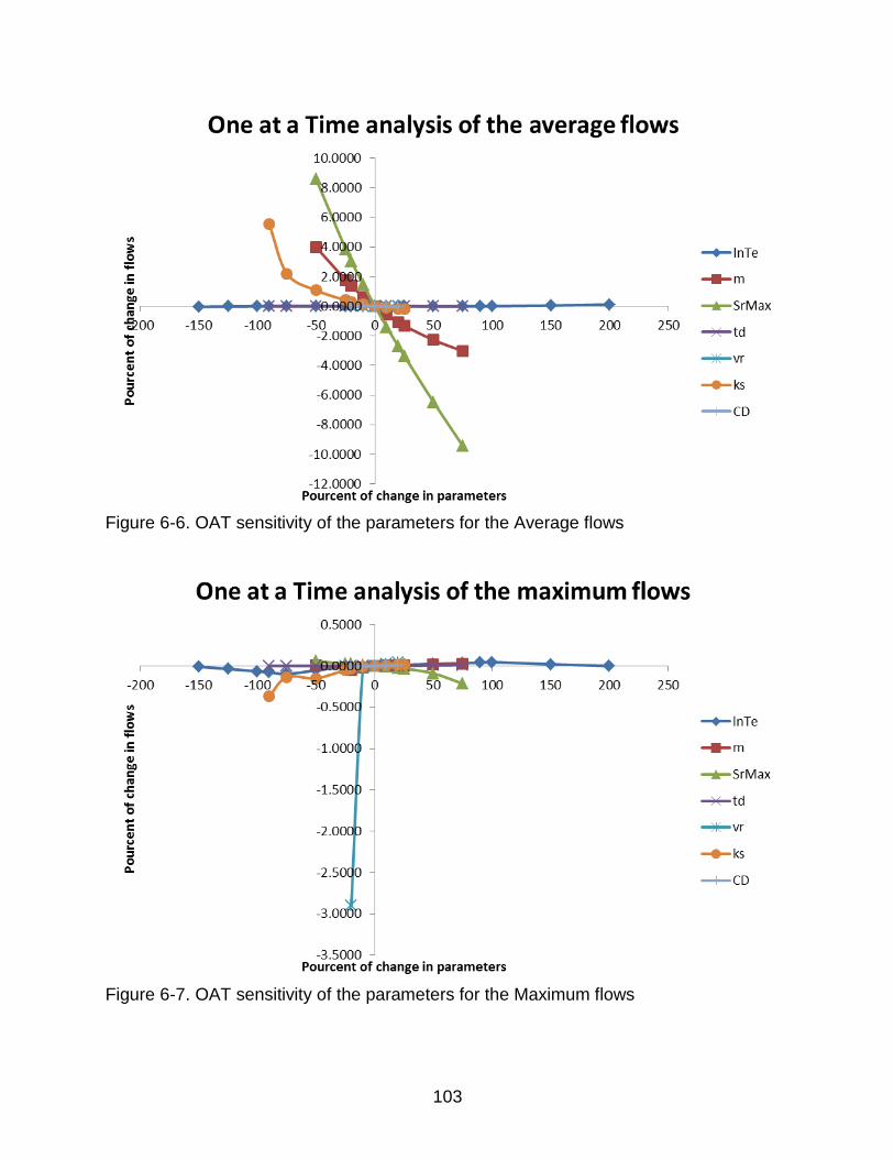
103
Figure 6-6. OAT sensitivity of the parameters for the Average flows
Figure 6-7. OAT sensitivity of the parameters for the Maximum flows

104
Figure 6-8. OAT sensitivity of the parameters for the Total flows

105
0
0.0005
0.001
0.0015
0.002
0.0025
0.003
0 0.0005 0.001 0.0015 0.002 0.0025 0.003
ᵟ
μ*
Morris Analysis for minimum flows
lnTe
m
SrMax
td
vr
ks
CD
Figure 6-9. Morris Sensitivity Index of the parameters for the minimum flows
0
0.01
0.02
0.03
0.04
0.05
0.06
0 0.01 0.02 0.03 0.04 0.05 0.06
ᵟ
μ*
Morris Analysis for median flows
lnTe
m
SrMax
td
vr
ks
CD
Figure 6-10. Morris Sensitivity Index of the parameters for the Median flows

106
0
0.01
0.02
0.03
0.04
0.05
0.06
0 0.01 0.02 0.03 0.04 0.05 0.06
δ
μ*
Morris analysis for average flows
lnTe
m
SrMax
td
vr
ks
CD
Figure 6-11. Morris Sensitivity Index of the parameters for the Average flows
0
0.005
0.01
0.015
0.02
0.025
0.03
0.035
0.04
0 0.005 0.01 0.015 0.02 0.025 0.03 0.035 0.04
ᵟ
μ*
Morris analysis for maximum flows
lnTe
m
SrMax
td
vr
ks
CD
Figure 6-12. Morris Sensitivity Index of the parameters for the maximum flows

107
0
100
200
300
400
500
600
700
800
0 100 200 300 400 500 600 700 800
ᵟ
μ*
Morris Analysis for total flows
lnTe
m
SrMax
td
vr
ks
CD
Figure 6-13. Morris Sensitivity Index of the parameters for the Total flows

108
Figure 6-14. FAST Sensitivity for the Total order indexes of the parameters
Figure 6-15. FAST Sensitivity for the First order indexes of the parameters

109
Figure 6-16. FAST Sensitivity for the interactions of the parameters

110
Figure 6-17. Probability distribution of the mimimum flows
Figure 6-18. Probability distribution of the median flows
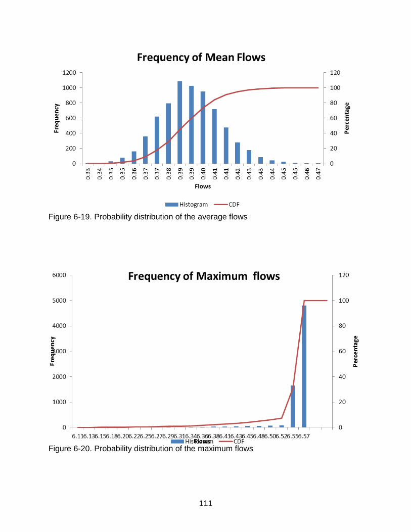
111
Figure 6-19. Probability distribution of the average flows
Figure 6-20. Probability distribution of the maximum flows

112
Figure 6-21. Probability distribution of the total flows

113
CHAPTER 7 CONCLUSIONS AND RECOMMENDATIONS
Conclusions
The implementation of TOPMODEL in R known as TOPMODEL package was
applied to the flood-prone River Grise basin to simulate the hydrological response of the
watershed and to determine the parameters of the model that can influence the most
this response.
As TOPMODEL tends to compute the areas that have contributed water to the
runoff process based on topographic index the downstream part of the catchment,
which is a flat area, seems not to be considered as contributing area. As a result, while
the total area of the watershed is about 393 km2, only approximately 290 km2 which
constitutes the catchment delineated by TOPMODEL (outlet different from the natural
outlet) was able to be processed in the hydrological simulation process. The
topographic index from the natural outlet could not be determined.
In fact, the topographic index which determines the hydrological similarity of each
part of the catchment is calculated as a function of the slope. Since estimating slopes in
flat areas is a critical issue (Pan, et al., 2004), r.topidx seems to assign null values to
the flat portion of the catchment.
In this study, the calculations and the Identification of parameters probability
distributions based on field data were attempted. Some parameters were calculated as
described in previous studies that have used TOPMODEL but, others such as the
scaling parameter that controls the rate of decline of transmissivity in the soil profile was
calculated by using soil data information from the literature.

114
Global and Local Sensitivity Analyses were performed in this study. The Local
sensitivity Analysis (LSA) allows the quantification of the effect of each input on the
overall output variance. It also indicates the range within the parameter can influence
the output the most The Global Sensitivity Analysis (GSA), mainly the FAST method,
allows the separation of first‐order versus total‐order effects
Both FAST and Morris methods that were used for the global sensitivity analysis
showed that the sensitivity varies with flows type neither all the parameters are not
sensitive. Only five (5) of them such as the transmissivity (lnTe), the scaling parameter
of the decline of transmissivity (m), Maximum root zone storage deficit (SrMax) the
hydraulic conductivity (ks) the channel velocity inside the catchment (vr) seem to
influence the runoff simulation of R-TOPMODEL. Also their influence seems to vary
whether the flows are low or high. Besides the hydraulic conductivity (ks), the moisture
deficit parameter (SrMax), and the rate of decline of the transmissivity with depth (m) that
seem to impact the hydrologic response of the catchment whether the flows are low
average or high, the channel velocity (vr) seems to specially impact high flows with no
impact on the total flows.
The sensitivity analyses results seem to confirm what other studies using
TOPMODEL have already revealed. According to Montesinos-Barrios and Beven
(2004), the model is very sensitive to the variations of the soil transmissivity decay
parameter, the soil transmissivity at saturation, the root zone storage capacity and the
channel routing velocity in large catchments. As demonstrated in this study, the
transmissivity (lnTe), the scaling parameter of the decline of transmissivity (m),
maximum root zone storage deficit (SrMax), the hydraulic conductivity (ks) are the most

115
sensitive parameters of TOPMODEL. The channel velocity inside the catchment (vr),
though less sensitive than the other previous parameters, is also sensitive for high
flows. Parameters such as the unsaturated zone time delay per unit storage deficit (td)
and capillary drive (CD) seem to have no influence on the output flow whatsoever. Is it
also remarkable that not all versions of TOPMODEL use this parameter (vr).
Morris is a qualitative screening method while FAST is a quantitative method that
confirmed the results from Morris.
Besides the maximums flows, the uncertainty analysis is quite similar for the rest
of the flows. They all present a relatively normal distribution sometimes skewed to the
left.
According to the uncertainty analysis, mimimum flows in the watershed is
expected to be in the range of null to 0.008 m3/3h. This seems to relate the situation on
the ground because the river has run out water in its lower part in some dry seasons
and cannot reach the natural outlet.
The average flows vary from 0.333 m3/3h to 0.467 m3/3h with an average of 0.390
m3/3h.The 95 % confidence interval lays within 0.357 m3/3h -0.427 m3/3h. However, the
cumulative distribution frequency (CDF) reveals that more than 85 % of the flows is
lower than 0.41 m3/3h.
The maximum flows presented a very particular shape compare to rest of the
flows. The 95% confidence interval varies within 6.403 m3/3h and 6.554 m3/3h. The
range of variability is goes from 6.107 m3/3h to 6.569 m3/3h with an average of
6.538m3/3h. The distribution of the frequency is very much skewed to the left. Most of

116
the distribution of frequency represents approximately 10 % of the cumulative
distribution function. The distribution seems to be lognormal.
It is important to notice that the hydraulic conductivity which is usually described
as lognormally distributed was processed as uniformly distributed in this study. The
equation of Kozeny-Carman has been used to determine the hydraulic conductivity.
Unlike others parameters which calculations methods have clearly shown their
distribution, no distribution pattern was observed for the hydraulic conductivity and was
processed as uniformally distributed.
Also the importance of the parameters can tell about management actions needed
to undertaken according to the management type that is pursuing. It was demonstrated
that the soil moisture deficit is inversely proportional to the flows and sould be increased
in a perspective of flood control for example. The m parameter which is related to the
recession curve is also very important in the watershed. The recession curve tells about
the amount of water that can be released in dry seasons and consequently help in
predicting the supporting amount of water to provide to satisfy the needs for
downstream activities in dry seasons.
Recommendations
This study aimed at determining the hydrological behavior of the River Grise
catchment using the implementation of the TOPMODEL in R. Attempts to define with
precision parameters of the model using field data available in the literature have been
made.
However, as presented in the results TOPMODEL seems to perform only for part
of the catchment. The outlet processed by the model is different from the natural outlet;
as a result a subcatchment representing the upstream of the watershed is delineated by

117
the model. This issue seems to be due to the flatness of the downstream of the
watershed. In fact, the topographic index calculation using the DEM seems not to
perform well in the flat area of the catchment. The quality of the DEM can also be
considered.
The performance of the model cannot be measured because there is no measured
flow data that is necessary to conduct the calibration and the validation which can
confirm the effectiveness of the TOPMODEL application to model the River Grise basin.
Besides the proper behavior of the parameters as revealed by their influence on the
flows, it is important to collect field flow data to perform calibration. The calibration
process will confirm the effectiveness of the TOPMODEL performance in the River
Grise watershed.
It is also important to notice that in the perspective of flood occurrence, it would be
important to analyze the stages in the watershed which this study did not consider.

118
APPENDIX A MORRIS CODE IN R
setwd("C:/Users/Joseph/Desktop/r.topmodel_ex/r.topmodel_ex/r.topmodel") library(topmodel) library(stinepack) library(e1071) library(Hmisc) library(sensitivity) library(zoo) library(xlsReadWrite) library(xts) library(matrixStats) DEM <- read.table("DEM2.txt") DEM <- as.matrix(DEM) DEM[DEM==-9999] <- NA library(lattice) #levelplot(DEM) # Fill sink0 DEM.filled <- sinkfill(DEM, res=30, degree=0.1) DEM.filled <- sinkfill(DEM.filled, res=30, degree=0.1) DEM.filled <- sinkfill(DEM.filled, res=30, degree=0.1) DEM.filled <- sinkfill(DEM.filled, res=30, degree=0.1) DEM.filled <- sinkfill(DEM.filled, res=30, degree=0.1) DEM.filled <- sinkfill(DEM.filled, res=30, degree=0.1) DEM.filled <- sinkfill(DEM.filled, res=30, degree=0.1) DEM.filled <- sinkfill(DEM.filled, res=30, degree=0.1) # View effect of filling sink0 difference <- DEM.filled - DEM # Calculate Topographic Index topindex <- topidx(DEM.filled, res=30) # View atb levelplot(topindex$atb) # View area levelplot(topindex$area) topindex <- make.classes(topindex$atb,16) # Note in the area plot that the highest contributing area is approximately # at row 381 and column 519 and not at 1,1. This is likely due to the lower # portion of the basin being very flat with no "clear" flow direction to be # found. In order to use the entire watershed, we may need to "burn" in the # river. # Calculate flow length and delay using the point with highest contributing # area. flowlength <- flowlength(DEM.filled, c(381,519)) * 30 flowlength <- hist(flowlength,5) delay <- data.frame(distance = flowlength$break0, area = c(0,flowlength$counts) / sum(flowlength$counts))

119
delay[,2] <- cumsum(delay[,2]) ##DATA UPLOADING ##3HRS DATA hrsweather<-read.table("Data3hrs.txt", header=FALSE, sep="\t") hrsrain <- hrsweather[,1] hrsET0<-hrsweather[,2] ##DAILY DATA dailyweather<-read.table("Datadaily.txt", header=FALSE, sep="\t") dailyrain <-dailyweather[,1] dailyET0<-dailyweather[,2] ## MONTHLY DATA Monthweather<-read.table("Datamonth.txt", header=FALSE, sep="\t") Monthrain <- Monthweather[,1] MonthET0<-Monthweather[,2] ##ANNUAL DATA Anweather<-read.table("Datayear.txt", header=FALSE, sep="\t") Anrain <- Anweather[,1] AnET0<-Anweather[,2] ##SIMULATION, MEAN , STANDARD DEVIATION AND CONFIDENCE INTERVAL CALCULATIONS ## MORRIS SIMULATION ##Parameters declaration param<-read.table("paramMorris.txt") qs0 <- 0.27 LnTe <- param[,1] m <- param[,2] Sr0 <- 0.01 Srmax <- param[,3] td <- param[,4] vch <- 4500 vr <- param[,5] k0 <- param[,6] CD <- param[,7] dt <- 3 Morrisparameters <- cbind(qs0, LnTe, m, Sr0, Srmax, td, vch, vr, k0, CD, dt) ##Simulation QsimhrsMorris <- topmodel(Morrisparameters, topindex, delay, hrsrain, hrsET0) SumhrsMorris<-colSums(QsimhrsMorris) ## Table of the outputs write.table(SumhrsMorris,"C:/Users/Joseph/Desktop/r.topmodel_ex/r.topmodel_ex/r.topmodel/ SumhrsMorris.xls", sep="\t") ##Table Means, Standard Deviation and Confidence Interval MeanhrsMorris<-colMeans(QsimhrsMorris) write.table(MeanhrsMorris,"C:/Users/Joseph/Desktop/r.topmodel_ex/r.topmodel_ex/r.topmodel/ MeanhrsMorris.xls", sep="\t")

120
StandarddevhrsMorris<-colSds(QsimhrsMorris) write.table(StandarddevhrsMorris,"C:/Users/Joseph/Desktop/r.topmodel_ex/r.topmodel_ex/r.topmodel/ StandarddevhrsMorris.xls", sep="\t") QMhrs0.025<-colQuantiles(QsimhrsMorris, probs=0.025) write.table(QMhrs0.025,"C:/Users/Joseph/Desktop/r.topmodel_ex/r.topmodel_ex/r.topmodel/ QMhrs0.025.xls", sep="\t") QMhrs0.50<-colQuantiles(QsimhrsMorris, probs=0.50) write.table(QMhrs0.50,"C:/Users/Joseph/Desktop/r.topmodel_ex/r.topmodel_ex/r.topmodel/ QMhrs0.50.xls", sep="\t") QMhrs0.975<-colQuantiles(QsimhrsMorris, probs=0.975) write.table(QMhrs0.975,"C:/Users/Joseph/Desktop/r.topmodel_ex/r.topmodel_ex/r.topmodel/ QMhrs0.975.xls", sep="\t") QMhrs1<-colQuantiles(QsimhrsMorris, probs=0.25) write.table(QMhrs1,"C:/Users/Joseph/Desktop/r.topmodel_ex/r.topmodel_ex/r.topmodel/ QMhrs1.xls", sep="\t") QMhrs3<-colQuantiles(QsimhrsMorris, probs=0.75) write.table(QMhrs3,"C:/Users/Joseph/Desktop/r.topmodel_ex/r.topmodel_ex/r.topmodel/ QMhrs3.xls", sep="\t") MinhrsMorris<-colMins(QsimhrsMorris) write.table(MinhrsMorris,"C:/Users/Joseph/Desktop/r.topmodel_ex/r.topmodel_ex/r.topmodel/ MinhrsMorris.xls", sep="\t") MaxhrsMorris<-colMaxs(QsimhrsMorris) write.table(MaxhrsMorris,"C:/Users/Joseph/Desktop/r.topmodel_ex/r.topmodel_ex/r.topmodel/ MaxhrsMorris.xls", sep="\t") SkewnesshrsMorris<-skewness(QsimhrsMorris) write.table(SkewnesshrsMorris,"C:/Users/Joseph/Desktop/r.topmodel_ex/r.topmodel_ex/r.topmodel/ SkewnesshrsMorris.xls", sep="\t") KurtosishrsMorris<-kurtosis(QsimhrsMorris) write.table(KurtosishrsMorris,"C:/Users/Joseph/Desktop/r.topmodel_ex/r.topmodel_ex/r.topmodel/ KurtosishrsMorris.xls", sep="\t") MeanhrsMorrismatrix<-mean(QsimhrsMorris) StandarddevhrsMorrisMatrix<- apply(QsimhrsMorris, 2, sd) QMhrs0.025Matrix<-quantile(QsimhrsMorris, probs=0.025) QMhrs0.50Matrix<-quantile(QsimhrsMorris, probs=0.50) QMhrs0.975Matrix<-quantile(QsimhrsMorris, probs=0.975) QMhrs1Matrix<-quantile(QsimhrsMorris, probs=0.25) QMhrs3Matrix<-quantile(QsimhrsMorris, probs=0.75) MinhrsMorrisMatrix<-min(QsimhrsMorris) MaxhrsMorrisMatrix<-max(QsimhrsMorris) SkewnesshrsMorrisMatrix<-skewness(QsimhrsMorris) KurtosishrsMorrisMatrix<-kurtosis(QsimhrsMorris) ## Uncertainty values MeanhrsMorrismatrix StandarddevhrsMorrisMatrix QMhrs0.025Matrix QMhrs0.50Matrix

121
QMhrs0.975Matrix QMhrs1Matrix QMhrs3Matrix MinhrsMorrisMatrix MaxhrsMorrisMatrix SkewnesshrsMorrisMatrix KurtosishrsMorrisMatrix

122
APPENDIX B FAST CODE IN R
Setwd ("C:/Users/Joseph/Desktop/r.topmodel_ex/r.topmodel_ex/r.topmodel") library(topmodel) library(stinepack) library(e1071) library(Hmisc) library(sensitivity) library(zoo) library(xlsReadWrite) library(xts) library(matrixStats) DEM <- read.table("DEM2.txt") DEM <- as.matrix(DEM) DEM[DEM==-9999] <- NA library(lattice) #levelplot(DEM) # Fill sink0 DEM.filled <- sinkfill(DEM, res=30, degree=0.1) DEM.filled <- sinkfill(DEM.filled, res=30, degree=0.1) DEM.filled <- sinkfill(DEM.filled, res=30, degree=0.1) DEM.filled <- sinkfill(DEM.filled, res=30, degree=0.1) DEM.filled <- sinkfill(DEM.filled, res=30, degree=0.1) DEM.filled <- sinkfill(DEM.filled, res=30, degree=0.1) DEM.filled <- sinkfill(DEM.filled, res=30, degree=0.1) DEM.filled <- sinkfill(DEM.filled, res=30, degree=0.1) # View effect of filling sink0 difference <- DEM.filled - DEM # Calculate Topographic Index topindex <- topidx(DEM.filled, res=30) # View atb levelplot(topindex$atb) # View area levelplot(topindex$area) topindex <- make.classes(topindex$atb,16) # Note in the area plot that the highest contributing area is approximately # at row 381 and column 519 and not at 1,1. This is likely due to the lower # portion of the basin being very flat with no "clear" flow direction to be # found. In order to use the entire watershed, we may need to "burn" in the # river. # Calculate flow length and delay using the point with highest contributing # area. flowlength <- flowlength(DEM.filled, c(381,519)) * 30 flowlength <- hist(flowlength,5)

123
delay <- data.frame(distance = flowlength$break0, area = c(0,flowlength$counts) / sum(flowlength$counts)) delay[,2] <- cumsum(delay[,2]) ##DATA UPLOADING ##3HRS DATA hrsweather<-read.table("Data3hrs.txt", header=FALSE, sep="\t") hrsrain <- hrsweather[,1] hrsET0<-hrsweather[,2] ##DAILY DATA dailyweather<-read.table("Datadaily.txt", header=FALSE, sep="\t") dailyrain <-dailyweather[,1] dailyET0<-dailyweather[,2] ##FAST SIMULATION ##Parmeters declaration param<-read.table("paramFAST.txt") qs0 <- 0.27 LnTe <- param[,1] m <- param[,2] Sr0 <- 0.01 Srmax <- param[,3] td <- param[,4] vch <- 4500 vr <- param[,5] k0 <- param[,6] CD <- param[,7] dt <- 3 Fastparameters <- cbind(qs0, LnTe, m, Sr0, Srmax, td, vch, vr, k0, CD, dt) ##Simulation of the outputs Qsimhrsfast <- topmodel(Fastparameters, topindex, delay, hrsrain, hrsET0) Sumhrsfast<-colSums(Qsimhrsfast) ##Tables of the outputs write.table(Sumhrsfast,"C:/Users/Joseph/Desktop/r.topmodel_ex/r.topmodel_ex/r.topmodel/ Sumhrsfast.xls", sep="\t") Meanhrsfast<-colMeans(Qsimhrsfast) write.table(Meanhrsfast,"C:/Users/Joseph/Desktop/r.topmodel_ex/r.topmodel_ex/r.topmodel/ Meanhrsfast.xls", sep="\t") Qhrs0.10fast<- colQuantiles(Qsimhrsfast, probs=0.10) write.table(Qhrs0.10fast,"C:/Users/Joseph/Desktop/r.topmodel_ex/r.topmodel_ex/r.topmodel/ Qhrs0.10fast.xls", sep="\t") Qhrs0.025fast<-colQuantiles(Qsimhrsfast, probs=0.025) write.table(Qhrs0.025fast,"C:/Users/Joseph/Desktop/r.topmodel_ex/r.topmodel_ex/r.topmodel/ Qhrs0.025fast.xls", sep="\t") Qhrs0.50fast<-colQuantiles(Qsimhrsfast, probs=0.50)

124
write.table(Qhrs0.50fast,"C:/Users/Joseph/Desktop/r.topmodel_ex/r.topmodel_ex/r.topmodel/ Qhrs0.50fast.xls", sep="\t") Qhrs0.50fast<- colQuantiles(Qsimhrsfast, probs=0.50) write.table(Qhrs0.50fast,"C:/Users/Joseph/Desktop/r.topmodel_ex/r.topmodel_ex/r.topmodel/ Qhrs0.50fast.xls", sep="\t") Qhrs0.975fast<-colQuantiles(Qsimhrsfast, probs=0.975) write.table(Qhrs0.975fast,"C:/Users/Joseph/Desktop/r.topmodel_ex/r.topmodel_ex/r.topmodel/ Qhrs0.975fast.xls", sep="\t") Qhrs1fast<-colQuantiles(Qsimhrsfast, probs=0.25) write.table(Qhrs1fast,"C:/Users/Joseph/Desktop/r.topmodel_ex/r.topmodel_ex/r.topmodel/ Qhrs1fast.xls", sep="\t") Qhrs3fast<-colQuantiles(Qsimhrsfast, probs=0.75) write.table(Qhrs3fast,"C:/Users/Joseph/Desktop/r.topmodel_ex/r.topmodel_ex/r.topmodel/ Qhrs3fast.xls", sep="\t") Minhrsfast<-colMins(Qsimhrsfast) write.table(Minhrsfast,"C:/Users/Joseph/Desktop/r.topmodel_ex/r.topmodel_ex/r.topmodel/ Minhrsfast.xls", sep="\t") Maxhrsfast<-colMaxs(Qsimhrsfast) write.table (Maxhrsfast,"C:/Users/Joseph/Desktop/r.topmodel_ex/r.topmodel_ex/r.topmodel/ Maxhrsfast.xls", sep="\t") Skewnesshrsfast<-skewness(Qsimhrsfast) write.table(Skewnesshrsfast,"C:/Users/Joseph/Desktop/r.topmodel_ex/r.topmodel_ex/r.topmodel/ Skewnesshrsfast.xls", sep="\t") Kurtosishrsfast<-kurtosis(Qsimhrsfast) write.table(Kurtosishrsfast,"C:/Users/Joseph/Desktop/r.topmodel_ex/r.topmodel_ex/r.topmodel/ Kurtosishrsfast.xls", sep="\t") Meanhrsfastmatrix<-mean(Qsimhrsfast) StandarddevhrsfastMatrix<- apply(Qsimhrsfast, 2, sd) Qhrs0.025fastMatrix<-quantile(Qsimhrsfast, probs=0.025) Qhrs0.50fastMatrix<-quantile(Qsimhrsfast, probs=0.50) Qhrs0.975fastMatrix<-quantile(Qsimhrsfast, probs=0.975) Qhrs1fastMatrix<-quantile(Qsimhrsfast, probs=0.25) Qhrs3fastMatrix<-quantile(Qsimhrsfast, probs=0.75) MinhrsfastMatrix<-min(Qsimhrsfast) MaxhrsfastMatrix<-max(Qsimhrsfast) SkewnesshrsfastMatrix<-skewness(Qsimhrsfast) KurtosishrsfastMatrix<-kurtosis(Qsimhrsfast) ## Uncertainty values Meanhrsfastmatrix StandarddevhrsfastMatrix Qhrs0.025fastMatrix Qhrs0.50fastMatrix Qhrs0.975fastMatrix Qhrs1fastMatrix

125
Qhrs3fastMatrix MinhrsfastMatrix MaxhrsfastMatrix SkewnesshrsfastMatrix KurtosishrsfastMatrix

126
APPENDIX C MATLAB CODE
C1. MATLAB CODE A
%Program to write file in desired SIMLAB format for temporal output clear all; clc; [data]=xlsread('Qhrsfast.xlsx'); [n,m]=size(data); %data(1:n-1,1:m)=data(2:n,1:m) fid=fopen('Qhrsfast.out','w');%Chage output file nme as required fprintf(fid,'%d\n',m); fprintf(fid,'QMinimum\n'); fprintf(fid,'Q0025\n'); fprintf(fid,'Q010\n'); fprintf(fid,'Q025\n'); fprintf(fid,'Q050\n'); fprintf(fid,'QMean\n'); fprintf(fid,'Q075\n'); fprintf(fid,'Q090\n'); fprintf(fid,'Q0975\n'); fprintf(fid,'QMaximum\n'); fprintf(fid,'QTotal\n'); fprintf(fid,'Q090010\n'); fprintf(fid,'Q090050\n'); fprintf(fid,'Q050040n'); fprintf(fid,'time = no\n'); fprintf(fid,'%d\n',n); for j=1:n fprintf(fid,'%4.4f %4.4f %4.4f %4.4f %4.4f %4.4f %4.4f %4.4f %4.4f %4.4f %4.4f %4.4f %4.4f %4.4f\n',data(j,1),data(j,2),data(j,3), data(j,4),data(j,5),data(j,6),data(j,7),data(j,8),data(j,9),data(j,10),data(j,11),data(j,12),data(j,13),data(j,14)); end fclose(fid);

127
C2. MATLAB CODE B % Read in 3 hours temperature files and abstract the daily maximum and minimum temperature % and calculate the daily mean temperautre, and then concatenate into three % single files clear; directory = pwd; % Need to be changed if different path newdir = [directory,'/processed']; cd (newdir) dayPosition =1; % Day 1 is 1/1/1979 %Need to be changed if different grids; [y,x,days] aPCP = NaN(3,2,97880); for i=1979:2012 year = int2str(i); fileName = ['apcp.HaitiBV.',year,'.nc']; % abstract data lat = nc_varget(fileName,'lat'); % 3 pts currently lon = nc_varget(fileName,'lon'); % 2 pts currently time = nc_varget(fileName,'time' ); % 3 hours time-step T3hrs = nc_varget(fileName,'apcp'); % Has dimensions: (3,2,time) T3hrs(T3hrs<0)=0; maxTime = max(time); aPCP(:,:,dayPosition:dayPosition+maxTime-1) = T3hrs; dayPosition = dayPosition+maxTime; end days = 722816:0.125:735050; % Matlab serial dates, 1/1/1979 - 6/30/2012 days = days'; %% Write to mean temperature file cd (directory); newFileName=('PCP_HaitiBV.nc');

128
% Add dimensions and sizes nc_create_empty ( newFileName ) nc_add_dimension ( newFileName, 'lat', 3 ) nc_add_dimension ( newFileName, 'lon', 2 ) nc_add_dimension ( newFileName, 'days', 97880 ) varstruct.Name = 'aPCP'; varstruct.Nctype = nc_double; varstruct.Dimension = {'lat','lon','days'}; nc_addvar ( newFileName, varstruct ) lon_varstruct.Name = 'lon'; lon_varstruct.Nctype = nc_float; lon_varstruct.Dimension = { 'lon' }; nc_addvar ( newFileName, lon_varstruct ) lat_varstruct.Name = 'lat'; lat_varstruct.Nctype = nc_float; lat_varstruct.Dimension = { 'lat' }; nc_addvar (newFileName, lat_varstruct ) day_varstruct.Name = 'days'; day_varstruct.Nctype = nc_double; day_varstruct.Dimension = { 'days' }; nc_addvar ( newFileName, day_varstruct ) % Add the subset of data to the new netcdf file nc_varput ( newFileName, 'lat', lat ); nc_varput ( newFileName, 'lon', lon ); nc_varput ( newFileName, 'aPCP', aPCP ); nc_varput ( newFileName, 'days', days ); % Add attributes nc_attput ( newFileName, 'aPCP', 'units', 'kg/m^2'); nc_attput ( newFileName, 'aPCP', 'var_desc', '3 hourly precipitation'); nc_attput ( newFileName, 'days', 'units', 'matlab serial date'); nc_attput ( newFileName, 'lat', 'units', 'degrees_north'); nc_attput ( newFileName, 'lat', 'long_name', 'Latitude' ); nc_attput ( newFileName, 'lat', 'actual_range', '18.83 18.33 f'); nc_attput ( newFileName, 'lon', 'units', 'degrees_east'); nc_attput ( newFileName, 'lon', 'long_name', 'Longitude' ); nc_attput ( newFileName, 'lon', 'actual_range', '287.64 287.89 f');

129
C3. MATLAB CODE C
% Read in 3 hours temperature files and abstract the daily maximum and minimum temperature % and calculate the daily mean temperautre, and then concatenate into three % single files clear; directory = pwd; % Need to be changed if different path newdir = [directory,'/processed']; cd (newdir) dayPosition =1; % Day 1 is 1/1/1979 %Need to be changed if different grids; [y,x,days] apevap = NaN(3,2,97880); for i=1979:2012 year = int2str(i); fileName = ['pevap.HaitiBV.',year,'.nc']; % abstract data lat = nc_varget(fileName,'lat'); % 3 pts currently lon = nc_varget(fileName,'lon'); % 2 pts currently time = nc_varget(fileName,'time' ); % 3 hours time-step T3hrs = nc_varget(fileName,'pevap'); % Has dimensions: (3,2,time) T3hrs(T3hrs<0)=0; maxTime = max(time); apevap(:,:,dayPosition:dayPosition+maxTime-1) = T3hrs; dayPosition = dayPosition+maxTime; end days = 722816:735050; % Matlab serial dates, 1/1/1979 - 6/30/2012 days = days'; %% Write to mean temperature file cd (directory); newFileName=('pevap_HaitiBV.nc'); % Add dimensions and sizes nc_create_empty ( newFileName ) nc_add_dimension ( newFileName, 'lat', 3 )

130
nc_add_dimension ( newFileName, 'lon', 2 ) nc_add_dimension ( newFileName, 'days', 97880 ) varstruct.Name = 'pevap'; varstruct.Nctype = nc_double; varstruct.Dimension = {'lat','lon','days'}; nc_addvar ( newFileName, varstruct ) lon_varstruct.Name = 'lon'; lon_varstruct.Nctype = nc_float; lon_varstruct.Dimension = { 'lon' }; nc_addvar ( newFileName, lon_varstruct ) lat_varstruct.Name = 'lat'; lat_varstruct.Nctype = nc_float; lat_varstruct.Dimension = { 'lat' }; nc_addvar (newFileName, lat_varstruct ) day_varstruct.Name = 'days'; day_varstruct.Nctype = nc_double; day_varstruct.Dimension = { 'days' }; nc_addvar ( newFileName, day_varstruct ) % Add the subset of data to the new netcdf file nc_varput ( newFileName, 'lat', lat ); nc_varput ( newFileName, 'lon', lon ); nc_varput ( newFileName, 'pevap', apevap ); % Add attributes nc_attput ( newFileName, 'pevap', 'units', 'kg/m^2'); nc_attput ( newFileName, 'pevap', 'var_desc', '3 hourly potential evaporation'); nc_attput ( newFileName, 'days', 'units', 'matlab serial date'); nc_attput ( newFileName, 'lat', 'units', 'degrees_north'); nc_attput ( newFileName, 'lat', 'long_name', 'Latitude' ); nc_attput ( newFileName, 'lat', 'actual_range', '18.83 18.33 f'); nc_attput ( newFileName, 'lon', 'units', 'degrees_east'); nc_attput ( newFileName, 'lon', 'long_name', 'Longitude' ); nc_attput ( newFileName, 'lon', 'actual_range', '287.64 287.89 f');

131
C4. MATLAB CODE D
% This code reads the NARR 3 hours time step precipitation data, access a subset of grid points, and then % creates new netcdf files %% clear all, close all dir = pwd; datatype = 'apcp'; %extracting 3 hours precipitation data for i=1979:2012 if ((i==1980)||(i==1984)||(i==1988)||(i==1992)||(i==1996)||(i==2000)||(i==2004)||(i==2008)) time = 2928; elseif (i==2012) time = 1456; % This is here since our ftp download only included data to 6/30/2012 else time = 2920; end %% Access NARR data directory = [dir,'/accumulated precipitation 3 hourly']; % Need to be changed if different cd (directory) % air = (y, x, time) [349,277,2920] for each nonlead year % time = hours since 1/1/1 0:00:00 in 3 hour increments % y = meters (0 to 8959788) at 32463m (mean) increments % x = meters (0 to 11297120) at 32463m (mean) increments % the projection coodinate is Lambert Conformal Format % the sourthwest corner is set as (0,0) % y is northward distance from southwest corner of domain in projection coordinates % x is eastward distance from southwest corner of domain in projection coordinates % each grid has its corresponding lon and lat. Corners of this grid are 12.2N; 133.5W, 54.5N; 152.9W, 57.3N; 49.4W, 14.3N; 65.1W. % degreesEast = (180 - degreesWest) + 180 year = int2str(i); fileName = [datatype,'.',year,'.nc']; % Need to change for other variables

132
% Create a 0.25 degree lat-lon grids to do projection later % Need to be changed for other grids x = 287.64:0.25:287.89; y = [18.83:-0.25:18.33]'; % Create a year precipitation array maxX = length(x); maxY = length(y); T3hrs = NaN(maxY,maxX,time); for dayi=0:8:time-8 ncid = netcdf.open(fileName,'NC_NOWRITE'); %For the temperautre data, the varid is 5 from year 1979 to 2002. The latitude %varid is 0 and the longitude varid is 1. if i>=1979 && i<=2002 thisLat = netcdf.getVar(ncid,0); thisLon = netcdf.getVar(ncid,1); data = double(netcdf.getVar(ncid,5,[0 0 dayi],[349,277,8])); % Units of K missingValue = netcdf.getAtt(ncid, 5, 'missing_value' ); fillValue = netcdf.getAtt(ncid, 5, '_FillValue' ); % Replace with NaN iMissing = find(data == missingValue); data(iMissing)=nan; iFill = find(data == fillValue); data(iMissing)=nan; % Apply scale and offset scaleFactor = netcdf.getAtt(ncid, 5, 'scale_factor' ); addOffset = netcdf.getAtt(ncid, 5, 'add_offset' ); elseif i>=2003 && i<=2007 thisLat = netcdf.getVar(ncid,0); thisLon = netcdf.getVar(ncid,1); data = double(netcdf.getVar(ncid,4,[0 0 dayi],[349,277,8])); % Units of K missingValue = netcdf.getAtt(ncid, 4, 'missing_value' ); fillValue = netcdf.getAtt(ncid, 4, '_FillValue' );

133
% Replace with NaN iMissing = find(data == missingValue); data(iMissing)=nan; iFill = find(data == fillValue); data(iMissing)=nan; % Apply scale and offset scaleFactor = netcdf.getAtt(ncid, 4, 'scale_factor' ); addOffset = netcdf.getAtt(ncid, 4, 'add_offset' ); elseif i>=2008 thisLat = netcdf.getVar(ncid,1); thisLon = netcdf.getVar(ncid,2); data = double(netcdf.getVar(ncid,7,[0 0 dayi],[349,277,8])); % Units of K missingValue = netcdf.getAtt(ncid, 7, 'missing_value' ); fillValue = netcdf.getAtt(ncid, 7, '_FillValue' ); % Replace with NaN iMissing = find(data == missingValue); data(iMissing)=nan; iFill = find(data == fillValue); data(iMissing)=nan; % Apply scale and offset scaleFactor = netcdf.getAtt(ncid, 7, 'scale_factor' ); addOffset = netcdf.getAtt(ncid, 7, 'add_offset' ); end data = data*scaleFactor; data = data+addOffset; % change data to double data = double(data); %% Close File netcdf.close(ncid); % Convert all negative longitudes to positive iNeg = find(thisLon < 0); thisLon(iNeg) = thisLon(iNeg)*-1; thisLon(iNeg) = (180-thisLon(iNeg)) +180;

134
% Interpolate to a regular grid so it is easier to just access the points % we want thisLon = double(thisLon); thisLat = double(thisLat); maxTime = size(data,3); data2 = nan(maxY,maxX,maxTime); for j=1:8 % Could do this for all days data2(:,:,j) = griddata(thisLon,thisLat,data(:,:,j),x,y,'linear'); end T3hrs(:,:,dayi+1:dayi+8) = data2; end timeNumber = [1:time]'; %% Create 3 hours precipitation and give it dimensions, dimension sizes, and attributes cd ('D:\Di\NARR data for Joseph\processed') newfileName = ['apcp.HaitiBV.',year,'.nc']; % Add dimensions and sizes nc_create_empty ( newfileName ) nc_add_dimension ( newfileName, 'lat', maxY ) nc_add_dimension ( newfileName, 'lon', maxX ) nc_add_dimension ( newfileName, 'time', time ) %These attributes are the same as the GFS dataset varstruct.Name = datatype; varstruct.Nctype = nc_double; varstruct.Dimension = { 'lat','lon','time'}; nc_addvar ( newfileName, varstruct ) lon_varstruct.Name = 'lat'; lon_varstruct.Nctype = nc_float; lon_varstruct.Dimension = { 'lat' }; nc_addvar ( newfileName, lon_varstruct ) lat_varstruct.Name = 'lon'; lat_varstruct.Nctype = nc_float; lat_varstruct.Dimension = { 'lon' }; nc_addvar (newfileName, lat_varstruct ) time_varstruct.Name = 'time'; time_varstruct.Nctype = nc_double;

135
time_varstruct.Dimension = { 'time' }; nc_addvar ( newfileName, time_varstruct ) % Add the subset of data to the new netcdf file nc_varput ( newfileName, datatype, T3hrs ); nc_varput ( newfileName, 'lat', y ); nc_varput ( newfileName, 'lon', x ); nc_varput ( newfileName, 'time', timeNumber ); % Add attributes nc_attput ( newfileName, datatype, 'units', 'kg/m^2'); %nc_attput ( newfileName, datatype, '_FillValue', '-32767 s'); %nc_attput ( newfileName, datatype, 'scale_factor','0.010000 f'); nc_attput ( newfileName, datatype, 'var_desc', '3 hours accumulated potential evaporation'); %nc_attput ( newfileName, datatype, 'add_offset', '327.649994 f'); %nc_attput ( newfileName, datatype, 'missing_value', '32766 s'); nc_attput ( newfileName, 'lat', 'units', 'degrees_north'); nc_attput ( newfileName, 'lat', 'long_name', 'Latitude' ); nc_attput ( newfileName, 'lat', 'actual_range', '18.83 18.33 f'); % Needs to be changed for different gridpoints nc_attput ( newfileName, 'lon', 'units', 'degrees_east'); nc_attput ( newfileName, 'lon', 'long_name', 'Longitude' ); nc_attput ( newfileName, 'lon', 'actual_range', '287.64 287.89 f'); % Needs to be changed for different gridpoints nc_attput ( newfileName, 'time', 'units', 'hours since 1-1-1 00:00:0.0'); nc_attput ( newfileName, 'time', 'steps', '3 hours time step'); en

136
C5. MATLAB CODE E
% This code reads the NARR 3 hours time step temperature data, access a subset of grid points, and then % creates new netcdf files %% clear all, close all dir = pwd; datatype = 'pevap'; %extracting 3 hours temperature data for i=1979:2004 if ((i==1980)||(i==1984)||(i==1988)||(i==1992)||(i==1996)||(i==2000)||(i==2004)||(i==2008)) time = 2928; elseif (i==2012) time = 1456; % This is here since our ftp download only included data to 6/30/2012 else time = 2920; end %% Access NARR data directory = [dir,'/accumulated potential evaporation 3 hourly']; % Need to be changed if different cd (directory) % air = (y, x, time) [349,277,2920] for each nonlead year % time = hours since 1/1/1 0:00:00 in 3 hour increments % y = meters (0 to 8959788) at 32463m (mean) increments % x = meters (0 to 11297120) at 32463m (mean) increments % the projection coodinate is Lambert Conformal Format % the sourthwest corner is set as (0,0) % y is northward distance from southwest corner of domain in projection coordinates % x is eastward distance from southwest corner of domain in projection coordinates % each grid has its corresponding lon and lat. Corners of this grid are 12.2N; 133.5W, 54.5N; 152.9W, 57.3N; 49.4W, 14.3N; 65.1W. % degreesEast = (180 - degreesWest) + 180 year = int2str(i); fileName = [datatype,'.',year,'.nc']; % Need to change for other variables

137
% Create a 0.25 degree lat-lon grids to do projection later % Need to be changed for other grids x = 287.64:0.25:287.89; y = [18.83:-0.25:18.33]'; % Create a year temperature array maxX = length(x); maxY = length(y); T3hrs = NaN(maxY,maxX,time); for dayi=0:8:time-8 ncid = netcdf.open(fileName,'NC_NOWRITE'); %For the temperautre data, the varid is 5 from year 1979 to 2002. The latitude %varid is 0 and the longitude varid is 1. if i>=1979 && i<=2007 thisLat = netcdf.getVar(ncid,0); thisLon = netcdf.getVar(ncid,1); data = double(netcdf.getVar(ncid,5,[0 0 dayi],[349,277,8])); % Units of K missingValue = netcdf.getAtt(ncid, 5, 'missing_value' ); fillValue = netcdf.getAtt(ncid, 5, '_FillValue' ); % Replace with NaN iMissing = find(data == missingValue); data(iMissing)=nan; iFill = find(data == fillValue); data(iMissing)=nan; % Apply scale and offset scaleFactor = netcdf.getAtt(ncid, 5, 'scale_factor' ); addOffset = netcdf.getAtt(ncid, 5, 'add_offset' ); elseif i>=2008 thisLat = netcdf.getVar(ncid,1); thisLon = netcdf.getVar(ncid,2); data = double(netcdf.getVar(ncid,7,[0 0 dayi],[349,277,8])); % Units of K missingValue = netcdf.getAtt(ncid, 7, 'missing_value' );

138
fillValue = netcdf.getAtt(ncid, 7, '_FillValue' ); % Replace with NaN iMissing = find(data == missingValue); data(iMissing)=nan; iFill = find(data == fillValue); data(iMissing)=nan; % Apply scale and offset scaleFactor = netcdf.getAtt(ncid, 7, 'scale_factor' ); addOffset = netcdf.getAtt(ncid, 7, 'add_offset' ); end data = data*scaleFactor; data = data+addOffset; % change data to double data = double(data); %% Close File netcdf.close(ncid); % Convert all negative longitudes to positive iNeg = find(thisLon < 0); thisLon(iNeg) = thisLon(iNeg)*-1; thisLon(iNeg) = (180-thisLon(iNeg)) +180; % Interpolate to a regular grid so it is easier to just access the points % we want thisLon = double(thisLon); thisLat = double(thisLat); maxTime = size(data,3); data2 = nan(maxY,maxX,maxTime); for j=1:8 % Could do this for all days data2(:,:,j) = griddata(thisLon,thisLat,data(:,:,j),x,y,'linear'); end T3hrs(:,:,dayi+1:dayi+8) = data2; end timeNumber = [1:time]';

139
%% Create 3 hours temperature and give it dimensions, dimension sizes, and attributes cd ('D:\Di\NARR data for Joseph\processed') newfileName = ['pevap.HaitiBV.',year,'.nc']; % Add dimensions and sizes nc_create_empty ( newfileName ) nc_add_dimension ( newfileName, 'lat', maxY ) nc_add_dimension ( newfileName, 'lon', maxX ) nc_add_dimension ( newfileName, 'time', time ) %These attributes are the same as the GFS dataset varstruct.Name = datatype; varstruct.Nctype = nc_double; varstruct.Dimension = { 'lat','lon','time'}; nc_addvar ( newfileName, varstruct ) lon_varstruct.Name = 'lat'; lon_varstruct.Nctype = nc_float; lon_varstruct.Dimension = { 'lat' }; nc_addvar ( newfileName, lon_varstruct ) lat_varstruct.Name = 'lon'; lat_varstruct.Nctype = nc_float; lat_varstruct.Dimension = { 'lon' }; nc_addvar (newfileName, lat_varstruct ) time_varstruct.Name = 'time'; time_varstruct.Nctype = nc_double; time_varstruct.Dimension = { 'time' }; nc_addvar ( newfileName, time_varstruct ) % Add the subset of data to the new netcdf file nc_varput ( newfileName, datatype, T3hrs ); nc_varput ( newfileName, 'lat', y ); nc_varput ( newfileName, 'lon', x ); nc_varput ( newfileName, 'time', timeNumber ); % Add attributes nc_attput ( newfileName, datatype, 'units', 'kg/m^2'); %nc_attput ( newfileName, datatype, '_FillValue', '-32767 s'); %nc_attput ( newfileName, datatype, 'scale_factor','0.010000 f'); nc_attput ( newfileName, datatype, 'var_desc', '3 hours accumulated potential evaporation'); %nc_attput ( newfileName, datatype, 'add_offset', '327.649994 f'); %nc_attput ( newfileName, datatype, 'missing_value', '32766 s');

140
nc_attput ( newfileName, 'lat', 'units', 'degrees_north'); nc_attput ( newfileName, 'lat', 'long_name', 'Latitude' ); nc_attput ( newfileName, 'lat', 'actual_range', '18.83 18.33 f'); % Needs to be changed for different gridpoints nc_attput ( newfileName, 'lon', 'units', 'degrees_east'); nc_attput ( newfileName, 'lon', 'long_name', 'Longitude' ); nc_attput ( newfileName, 'lon', 'actual_range', '287.64 287.89 f'); % Needs to be changed for different gridpoints nc_attput ( newfileName, 'time', 'units', 'hours since 1-1-1 00:00:0.0'); nc_attput ( newfileName, 'time', 'steps', '3 hours time step'); end

141
APPENDIX D PARAMETERS CALCULATIONS
B 1058
n 4
ᵩe Calculated k0(mean)
by Kozenzy-Carman equation
lower limit μ
upper limit lower K0 μ upper
clay 0.28 0.14 0.269 0.385 0.501 0.055398 0.232449 0.666556 0.177051 0.434106
clayloam 0.36 0.46 0.279 0.39 0.501 0.064107 0.244762 0.666556 Sandy clay loam 0.61 0.945 0.235 0.33 0.425 0.032267 0.12547 0.345177
td 0.428821 3 4.797964
1.28694 3.082204
Srmax 0.31911 0.4495 0.57989
0.13039 0.13039
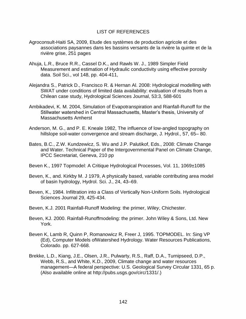
142
LIST OF REFERENCES
Agroconsult-Haiti SA, 2009, Etude des systèmes de production agricole et des associations paysannes dans les bassins versants de la rivière la quinte et de la rivière grise, 251 pages
Ahuja, L.R., Bruce R.R., Cassel D.K., and Rawls W. J., 1989 Simpler Field Measurement and estimation of Hydraulic conductivity using effective porosity data. Soil Sci., vol 148, pp. 404-411,
Alejandra S., Patrick D., Francisco R. & Hernan Al. 2008: Hydrological modelling with SWAT under conditions of limited data availability: evaluation of results from a Chilean case study, Hydrological Sciences Journal, 53:3, 588-601
Ambikadevi, K. M. 2004, Simulation of Evapotranspiration and Rianfall-Runoff for the Stillwater watershed in Central Massachusetts, Master’s thesis, University of Massachusetts Amherst
Anderson, M. G., and P. E. Kneale 1982, The influence of low-angled topography on hillslope soil-water convergence and stream discharge, J. Hydrol., 57, 65– 80.
Bates, B.C., Z.W. Kundzewicz, S. Wu and J.P. Palutikof, Eds., 2008: Climate Change and Water. Technical Paper of the Intergovernmental Panel on Climate Change, IPCC Secretariat, Geneva, 210 pp
Beven K., 1997 Topmodel: A Critique Hydrological Processes, Vol. 11, 1069±1085
Beven, K., and. Kirkby M. J 1979, A physically based, variable contributing area model of basin hydrology, Hydrol. Sci. J., 24, 43–69.
Beven, K., 1984. Infiltration into a Class of Vertically Non-Uniform Soils. Hydrological Sciences Journal 29, 425-434.
Beven, K.J. 2001 Rainfall-Runoff Modeling: the primer, Wiley, Chichester.
Beven, KJ. 2000. Rainfall-Runoffmodeling: the primer. John Wiley & Sons, Ltd. New York.
Beven K, Lamb R, Quinn P, Romanowicz R, Freer J, 1995. TOPMODEL. In: Sing VP (Ed), Computer Models ofWatershed Hydrology. Water Resources Publications, Colorado. pp. 627-668.
Brekke, L.D., Kiang, J.E., Olsen, J.R., Pulwarty, R.S., Raff, D.A., Turnipseed, D.P., Webb, R.S., and White, K.D., 2009, Climate change and water resources management—A federal perspective: U.S. Geological Survey Circular 1331, 65 p. (Also available online at http://pubs.usgs.gov/circ/1331/.)

143
Bois P., juin 2003, Hydraulique des écoulements en Rivière, notes de cours, Professor at the University of Grenoble.
Buytaert, W., De Bievre, B., Wyseure, G., Deckers, J., 2005. The effect of land use changes on the hydrological behaviour of Histic Andosols in south Ecuador. Hydrological Processes 19: 3985 -3997
Campling P., Gobin A., Beven K., Feyen J. 2002, Rainfall-runoff modelling of a humid tropical catchment: the TOPMODEL approach, Hydrol. Process. 16, 231–253 (2002), DOI: 10.1002/hyp.341
Cappus, P. (1960) Etude des lois de l'écoulement, application au calcul et à la prévision des débits. La Houille Blanche 60,493-520
Chan K., Saltelli A., Tarantola S. 1997 Sensitivity Analysis Of Model Output: Variance-Based Methods Make the Difference, Proceedings of the 1997 Winter Simulation Conference ed. S. Andradóttir, K. J. Healy, D. H. Withers, and B. L. Nelson. Environment Institute European Commission Joint Research Centre TP 272, 21020 Ispra (VA), ITALY
Chow, V.T., 1959 Open-channel hydraulics: New York, McGraw- Hill Book Co., 680 p.
Corral, C., 2004: Desenvolupament d'un model hidrològic per incorporar informació del radar meteorològic. Aplicació operacional a la conca del riu Besòs, Tesi Doctoral, Universitat Politècnica de Catalunya, 175 pp.
Cosby, B.J.,Hornberger G.M., Ginn T.R., and Clapp, R.B., 1984, A statistical exploration of the relationships of soil moisture characteristics to the physical properties of soils: Water Resources Research, v. 20,, p. 682-690
Cukier, R. I., Fortuin C. M., Schuler, K. E., Petscheck A. G. and Schailbly, J. H. (1973). Study of the sensitivity of coupled reaction systems to uncertainties in rate coefficients. I Theory. J.Chem. Phys. 59, 3873-3878
Cukier, R. I., Levine, H. B. and Schuler, K. E., 1978 Nonlinear analysis for multiparameter model systems. J. Comput. Phys. 26, 1-42
Cukier, R. I., Schailbly, J. H., and Schuler, K. E., 1975. Study of the sensitivity of coupled reaction systems to uncertainties in rate coefficients. . III. Analysis of the approximations. J.Chem. Phys. 63, 1140-1149
Dautrebande, S., Sohier, C. and Brahy, V. 2006.. L’érosion hydrique et les pertes en sols agricoles en Région Wallonne. Dossier scientifique réalisé dans le cadre du rapport analytique 2006-2007 sur l’état de l’environnement Wallon. FUSAGx-UHAGx Gembloux, 121p

144
Delusca K., 1998. Estimation de l’érosion hydrique des sols à l’aide de l’équation Universelle de Perte de sol assistée d’un système d’Information Géographique: Le cas du basin versant de la ravine Balan, Haiti. Université de Moncton 1-48
Dunne, T. and Black, R.D., 1970, An experimental investigation of runoff production in permeable soils, Water Resources Research, 6: 478-490
Durand, P, Robson, A, and Neal, C. 1992 Modelling the hydrology of submediterranean montain catchments (Mont Lozère, France), using TOPMODEL: initial results, J. Hydrol., 139, 1-14
Ekman, E.L. 1926. Botanizing in Haiti. U.S. Naval Med. Bull., 24(1):483-497.
Famiglietti, J.S., 1992, Aggregation and scaling of spatially-variable hydrological processes- Local, catchment-scale and macroscale models of water and energy balance: Princeton, Princeton University, October 1992, Ph.D. dissertation, 207 p.
Fedak R. 1999 Effect of Spatial Scale on Hydrologic Modeling in a Headwater Catchment, Master’s thesis, Virginia Polytechnic Institute and State University 179 p
Georges Y, 2008, Contribution à l'évaluation de l'érosion dans le bassin versant de la rivière Grise pour un meilleur plan d'aménagement. Faculte Universitaire des Sciences Agronomiques de Gembloux (FUSAGx). Mémoire de Master complementaire, 50p
Grabs T.; Seibert J.; Bishop K.; Laudon, H., 2009. Modeling spatial patterns of saturated areas: a comparison of the topographic wetness index and a dynamic distributed model. Journal of Hydrology, 373(1-2):15-23.
Graham, D.N. and M. B. Butts 2005 Flexible, integrated watershed modelling with MIKE SHE. In Watershed Models, Eds. V.P. Singh & D.K. Frevert Pages 245-272, CRC Press. ISBN: 0849336090.
Gupta, H.V., Sorroshian, S and Yapo, P.O (1999) Status of automatic calibration for hydrologic models: comparison with multilevel expert calibration, Journal of Hydrologic Engineering, ASCE, Vol. 4, No. 2, 135-143.
Haan, C. T. 2002. Statistical Methods in Hydrology. 2nd ed. Ames,Iowa: Iowa State University Press.
Hantush M. and Khalin L., 2003, Modeling Uncertainty of Runoff and Sediment Yield Using a Distributed Hydrologic Model
Haygarth P. M., Beven K. J., Joynes A., Butlerb T., Keelera C., Freera J., Owensc P. Wood G. Sampling for Assessing Risk to Water Quality,

145
Hewlett, J. D. and. Hibbert 1967 A. R, Factors affecting the response of small watersheds to precipitation in humid areas, in International Symposiumon Forest Hydrology (1965), Penn State University, edited by W. E. Sopper and H. W. Lull, pp. 275– 290, Pergamon, New York.
Hingray, B., Picouet, C., Musy, A. 2009 Hydrologie. 2. Une science pour l’ingénieur. Lausanne: Presses Polytechniques Universitaires Romandes.
Holdridge, L.R. 1947. The pine forest and adjacent mountain vegetation of Haiti considered from the standpoint of a new climatic classification of plant formations. Ph.D. Dissertation. Univ. Michigan, Ann Arbor, 186 pp.
Holly, G. 1999. Les problèmes environnementaux de la Région Métropolitaine de Portau-Prince. Commission pour la commémoration du 250eme anniversaire de la fondation de Port-au-Prince. Port-au-Prince, Haïti 221p.
Hornberger, G M, Beven, K J, Cosby, B J and Sappington, D E. 1985 Shenandoah Watershed Study: Calibration of a Topography-Based, Variable Contributing Area Hydrological Model to a Small Forested Catchment, Water Resour. Res. 21; 1841-1850.
Horton, RE., 1933. The role of infiltration in the hydrologic cycle, Transactions of the American Geophysical Union, 14: 446-460.
Johnstone D., and Cross W.P., 1949, Elements of Applied Hydrology, Ronald Press Company, New-York
Joseph A., Mai 2004, Rapport de synthèse des études de vulnérabilité et d’adaptation aux conditions climatiques externes en Haïti, secteurs: zones côtières, ressources en eau, risques et désastres, agriculture et désertification, 73 pages
Judd, W.S. 1987. Floristic study of Morne la Visite and Pic Macaya national parks, Haiti. Bulletin Florida State Museum, 32(1):1-136.
Knowles, R. B., Markley, B., Buckalew, J., Roebuck, L. W. (1999), Water Resources Assessment of Haiti,40p
Lalonde, Girouard, Letendre, and Associes, Ltd. 1977, Project d’Inventaires des Ressources Hydrauliques, Hydrogéologie Préliminaire de la Plaine de Cul-de-Sac. Vol. 110, Contract 444/00407, Montreal, Canada: Agence Canadienne de Developpement International, June 1977.
Lee G.*, Tachikawa Y., Takara K., 2006, Analysis of Hydrologic Model Parameter Characteristics Using Automatic Global Optimization Method, Annuals of Disas,Prev. Res. Inst., Kyoto Univ., No. 49 B,

146
Lettenmaier, D., D. Major, L. Poff, and S. Running, 2008. Water Resources. In: The effects of climate change on agriculture, land resources, water resources, and biodiversity in the United States. A Report by the U.S. Climate Change Science Program and the Subcommittee on Global Change Research. Washington, DC., USA, 362
MacFadden, BJ. 1986. Geological setting of Macaya and La Visite National Park0, southern peninsula of Haiti. Published Report. U.S. Agency for International Development, Haiti, Port-au-Prince, 33 pp.
Marco Franchiniav*, Jacques Wendlingbvl, Charles Obled”, Ezio Todini” 1996 Physical interpretation and sensitivity analysis of the TOPMODEL Journal of Hydrology 175 293-338
McCuen, R.H., Johnson, P.A., and Ragan, R.M., 2002, "Highway Hydrology," U.S. Department of Transportation, Federal Highway Administration, Hydraulic Design Series No. 2, FHWA-NHI-02-001, Second Edition
Montesinos-Barrios, P., Beven K. 2004, Evaluation of TOPMODEL http://s1004.ok0tate.edu/S1004/Regional-Bulletins/Modeling Bulletin/ TOPMODEL.html
Moreda F. 1999 Conceptual rainfall - runoff models for different time steps with special consideration for semi-arid and arid catchments. Laboratory of Hydrology, Faculty of Applied Sciences, VUB, Pleinlaan 2, 1050 Brussels, Belgium. Dissertation 208pp
Morel-Seytoux H. J, 1999, Soil water retention and maximum capillary drive from saturation to oven dryness WATER RESOURCES RESEARCH, VOL. 35, NO. 7, PAGES 2031-2041
Morel-Seytoux, H.J., Khanji, J., 1974. Derivation of an Equation of Infiltration. Water Resources Research, 10, 795-800.
Morgan, M. G., and M. Henrion. 1992. Uncertainty: A Guide to Dealing with Uncertainty in Quantitative Risk and Policy Analysis. Cambridge, U.K.: Cambridge University Press
Morris M. D. 1991, Factorial Sampling Plans for Preliminary Computational Experiments, Technometrics, vol 33, N0. 2. (May, 1991), pp. 161-174
Muletha, M.K. and Nicklow, J.W. (2005) Sensitivity and uncertainty analysis coupled with automatic calibration for a distributed watershed model, Journal of Hydrology 306, 127-145.
Musy, A. 2005 Cours d’hydrologie générale. HYDRAM – ISTE – Ecole Polytechnique Fédérale de Lausanne (EPFL), http://hydram.epfl.ch/e-drologie/.

147
Nourani V., Roughani A., Gebremichael M., (2011) Topmodel Capability for Rainfall-Runoff Modeling of The Ammameh Watershed At different time scales using different terrain algorithms, Journal of Urban and Environmental Engineering, v.5, n.1, p.1-14, ISSN 1982-3932 doi: 10.4090/juee.2011.v5n1.001014
Oliver J.E. and Hidore, J.J., 2002 Climatology, An Atmospheric Science, 2nd edn. Prentice Hall
Pan, F., C. D. Peters-Lidard, M. J. Sale, and A. W. King (2004), A comparison of geographical information systems–based algorithms for computing the TOPMODEL topographic index, Water Resour. Res., 40, W06303, doi:10.1029/2004WR003069.
Parsons J. E., Thomas D. l., Huffman R. L, 2004, Agricultural Non-Point source water quality Models, Their use and Application. A cooperative publication associated with CSREES and EWRI southern cooperative Series Bulletin # 398 ISBN: 1-58161-398-9
Pinol, J, Beven, K J and Freer, J, 1997, Modelling the hydrological response of Mediterranean catchments, Prades, Catalonia - the use of distributed models as aids to hypothesis formulation Hydrol. 11, 1287-1306
Projet Interuniversitaire Cible (PIC), 2008, Projet Pilote de support des zones habitables de Port-au-Prince. Feuille 1 - Pernier, 27 pages
Quinn, P., K. Beven, P. Chevallier, and O. Planchon, The prediction of hillslope flow paths for distributed hydrological modelling using digital terrain models, Hydrol. Processes, 5, 59-79, 1991
Rawls, W.J., and D. L. Brakensiek, A procedure to predict Green Ampt Infiltration Parameters, Adv. Infiltration , A. Soc. Agric. Eng., pp. 102-1983.
Rawls, W.J., and D. L. Brakensiek, and R. Savaki Estimation of soil properties, Trans. Am. Soc. Agric. Engrs., vol 25 no. 5, pp. 1316-1330, 1328, 1982 Properties J. Irrig. Drain. Emg., vol 108, no. IR2, pp. 166-171, 1982
Rawls, W.J., and D. L. Brakensiek, Prediction of Soil Water Properties for hydrologic Modeling, Watershed Management I eighties, ACE, pp. 293-299, 1985
Reed, Seann, Victor Koren, Michael Smith, Ziya Zhang, Fekadu Moreda, Dong-Jun Seo, and DMIP Participants (2004). “Overall Distributed Model Intercomparison Project Results.” Journal of Hydrology, 298, pp. 27-60.
Richard L. G. and Dennis A. S., 2004 Soil Profile Descriptions for Steeplands Research Sites in Haiti Auburn University, Alabama, 36849,5412 U.S.A. United States Agency for International Development, Soil Management Collaborative Research Support Program Auburn University, Technical Bulletin No. 2004,01

148
Robson, A J, Whitehead, P G and Johnson, R C. 1993 An application of a physically based semi-distributed model to the Balquhidder catchments, J. Hydrol., 145, 357-370
Rodriguez-Iturbe, I., and J. B. Valdes (1979), the geomorphic structure of Hydrologic response, Water Resources., 15(6), 1409–1420
Satelli, A. Tarantola, S., Campolongo F. Ratto, M. (2004), Sensitivity Analysis in Practice. A guide to Assessing Scientific, Models Wiley, 133 p
Saltelli, A., Chan K., Scott E.M. Eds (2000). Sensitivity Analysis. John Wiley and Sons,
Siebert, J., Bishop, K. H., and Nybert, L. 1997. `A test of TOPMODEL's ability to predict spatially distributed groundwater levels',Hydrol. Process., 11, 1131±1144.
Sempere-Torres, D, 1990, Calcul de la lame ruisselée dans la modélisation pluie-débit: limitations des approches globales et introduction simplifiée de la topographie et de la variabilité spatiale des pluies. These de Doctorat., Institut de Mécanique de Grenoble, France
Sergile F., 1998. Environnement naturel des bassins versants des rivieres Grise et Blanche. P. 9-40
Shirmohammadi, A., I. Chaubey, R. D. Harmel, D. D. Bosch, R. Munoz‐Carpena, C. Dharmasri, A. Sexton, M. Arabi, M. L. Wolfe, J. Frankenberger, C. Graff, and T. M. Sohrabi. 2006. Uncertainty in TMDL models. Trans. ASABE 49(4): 1033‐1049
Smith, S., E. and Hersey, D. 2008. Analysis of watershed vulnerability to flooding in Haiti.World applied sciences journal 4 (6):869-885
Sobol, I. M. 1990a. Sensitivity estimates for nonlinear mathematical models. Matematicheskoe Modelirovanie 2: 112{118 (in Russian).
Sobol, I. M. 1990b. Quasi-Monte-Carlo methods. Progress in Nuclear Energy 24: 5561.
Sobol, I.M. 1993, “Sensitivity Estimates for Nonlinear Mathematical Models,” Mathematical Modeling and Computation, 1(4):407-414.
Smith, Michael B., Dong-Jun Seo, Victor I. Koren, Seann M. Reed, Ziya Zhang, Qingyun Duan, Fekadu Moreda, Shuzheng Cong 2004b. “The Distributed Model Intercomparison Project (DMIP): Motivation and Experiment Design”. Journal of Hydrology, 298, pp. 4-26
Smucker G. R,Bannister M., D’Agnes Heather, Gossin Y., Portnoff M., Timyan J., Tobias S., Toussaint R., April 2007, Environmental Vulnerability in Haiti, 141 pp
Swartley D. B., Toussaint J. R., May 06, Haiti Country Analysis of Tropical Forestry and Biodiversity, 80 pages

149
Timyan J. C. 2006, Criteria for selecting watershed priority in Haiti, 17 pp
Timyan, J. C. 1999. Large-scale Hillside Re-vegetation of the Upper Grise and Blanche River Watersheds. Winrock International, Petion-Ville. 44 p
Page, T., Haygarth, P.M., Beven, K., Joynes, A., Butler, P., Keeler,C., Freer, J., Owens, P. & Woods, G. 2005. Spatial variability of soil phosphorus in relation to the topographic index and critical source areas: sampling for assessing risk to water quality. Journal of Environmental Quality, 34, 2263–2277
Wallach D., Makowski D. Jones J.W. 2006, Working with Dynamic Crop Models. Evaluation, Analysis, Parameterization, and Applications. Elsevier B. V. 444 pp
Wendling, J, 1992, Modélisation pluie-débit: comparaison d'approches conceptuelles/physico-déterministes, globales/semi-distribuées. Essai de prise en compte de la variabilité spatiale des pluies. (Application au bassin versant du Réal Collobrier). Thèse de Doctorat, Institut national polytechnique de Grenoble, France.
Wolock, D. M., and C. V. 1994 Price, Effects of digital elevation model map scale and data resolution on a topography-based watershed model, Water Resour. Res., 30, 3041-3052,
Wolock D. M., 1993,Simulating the variable source area concept of streamflow generation with watershed model TOPMODEL, US Geological Survey, water Resources Investigations Report 93-4124
Zhang, W., and D. R. Montgomery, Digital elevation model grid size, landscape representation, and hydrologic simulations, Water Resour. Res., 30, 1019-1028, 1994.

150
BIOGRAPHICAL SKETCH
Joseph Beneche was born in Les Coteaux (Damassin) which is in the South of
Haiti. He went to college St Jean des Cayes where he graduated from high school in
July 2000. In October of 2000, he moved to Port au Prince and successfully passed the
entrance exam at Faculté d’ Agronomie et de Médecine Vétérinaire (FAMV) of the State
University (UEH) where he spent five years and received his bachelor’s degree in
agricultural engineering. Over approximately the next five (5) years, Joseph worked
among 2 private consulting firms and an NGO, holding position ranging from being site
engineer to team leader. In July 2010, Joseph obtained a scholarship from USAID /
WINNER project to come to University of Florida (USA) where he receives his master’s
degree in agricultural and biological engineering with a concentration in hydrologic
sciences in May 2013. His skills include water project management, hydrological
modeling, computer programing. Joseph wants to be a long life learner in the field of
hydrology, work in challenging environments, and give back to his country through the
expertise he will have acquired.