UK/KRCEE Doc #: P12.1 2007

Sensitivity Analysis on the Half-Life of Trichloroethylene and the Distribution Coefficient at the

Paducah Gaseous Diffusion Plant

Prepared by Kentucky Research Consortium for Energy and Environment

233 Mining and Minerals Building University of Kentucky, Lexington, KY 40506-0107

Prepared for United States Department of Energy Portsmouth/Paducah Project Office

Acknowledgment: This material is based upon work supported by the Department of Energy under Award Number DE-FG05-03OR23032.

May 2007

UK/KRCEE Doc #: P12.1 2007

Sensitivity Analysis on the Half-Life of Trichloroethylene and the Distribution Coefficient at the

Paducah Gaseous Diffusion Plant

By

Joshua D. Kopp Summer 2007

University of Kentucky College of Engineering

Department of Civil Engineering Lexington, Kentucky

May 2007

ACKNOWLEDGEMENTS I would like to express my sincere gratitude and thanks to Dr. Lindell Ormsbee for

allowing me to work under his guidance and supervision. This project has been

challenging and has pushed me to my limits and beyond.

I would also like to sincerely thank Dr. Chandramouli Viswanathan. Without his help

and advice this project could not have come together as well as it has. His constant

encouragement and positive attitude always kept me striving to achieve greater heights

than I thought possible.

i

TABLE OF CONTENTS

FIGURES........................................................................................................................ iii TABLES ......................................................................................................................... iii ACRONYMS.................................................................................................................. iv 1.1 BACKGROUND ....................................................................................................... 1 1.2 AREA OF STUDY .................................................................................................... 2 1.3 MODEL DESCRIPTION .......................................................................................... 5

1.3.1 DESCRIPTION OF MODFLOWT .................................................................. 5 1.3.2 THE FINITE DIFFERENCE METHOD.......................................................... 6 1.3.3 STRESS PERIODS........................................................................................... 6 1.3.4 DESCRIPTION OF GROUNDWATER VISTAS ........................................... 7

1.4 MODEL VERIFICATION ........................................................................................ 7 1.5 SOURCES ................................................................................................................. 8 1.6 SUMMARY............................................................................................................. 10 2.1 PURPOSE OF THE ARTIFICIAL NEURAL NETWORK.................................... 11 2.2 ARTIFICIAL NEURAL NETWORKS................................................................... 11

2.1.1 TRAINING, TESTING, AND VALIDATION.............................................. 13 2.1.2 ACTIVATION FUNCTIONS ........................................................................ 13 2.1.3 TRAINING PROCESS................................................................................... 14

2.5 ANN MODELING SOFTWARE............................................................................ 15 2.3 DATASETS............................................................................................................. 15

2.3.1 INPUTS........................................................................................................... 15 2.3.2 OUTPUTS....................................................................................................... 16 2.3.3 SIMULATIONS ............................................................................................. 16

2.4 ARCHITECHTURE USED..................................................................................... 19 2.6 RESULTS ................................................................................................................ 20 2.7 DISCUSSION.......................................................................................................... 25

2.7.1 LIMITATIONS............................................................................................... 25 2.7.2 FUTURE INVESTIGATIONS....................................................................... 26

WORKS CITED ............................................................................................................ 31

ii

FIGURES Figure 1: Layout of the PGDP and Surrounding Areas Including the Modeled Existing

TCE Plume........................................................................................................ 3 Figure 2: Location of Wells in PGDP Site used in ANN Models ...................................... 4 Figure 3: Three-Dimensional Finite Difference Grid ......................................................... 6 Figure 4: Geologic Formations Underlying the PGDP (DOE 2005).................................. 8 Figure 5: Location of the Seven Primary UCRS Sources................................................... 9 Figure 6: Spatial Distribution of Initial TCE Concentrations in the RGA Under the C400

Building........................................................................................................... 10 Figure 7: General ANN Model Architecture .................................................................... 12 Figure 8: Graph of the Unipolar Activation Function ...................................................... 14 Figure 9: Artificial Neural Network (shown with 18 inputs) for One Observation Well. 19Figure 10: Predicted and Observed TCE Concentrations in OW Bayou-1 based on ANN

model OWB1-15............................................................................................. 21 Figure 11: Predicted and Observed TCE Concentrations in OW 5 based on ANN model

OW5-15........................................................................................................... 23 Figure 12: Predicted versus Observed TCE concentrations based on Model OWB1-15 . 27Figure 13: Predicted versus Observed TCE concentrations based on Model OW5-18.... 29

TABLES Table 1: Extraction Wells used in ANN Models Created to Determine Optimal Number

of Inputs ............................................................................................................. 16 Table 2: Pumping Simulations for each Dataset............................................................... 18 Table 3: Pumping Rates at Existing Extraction Wells (KRCEE 2007) ............................ 19 Table 4: ANN Parameter Values ...................................................................................... 20 Table 5: R2 Values from ANN Models for Observation Wells Bayou-1 and 5................ 20 Table 6: R2 Values from ANN Models for Individual Years ........................................... 25

iii

ACRONYMS ANN Artificial Neural Network ATSDR Agency for Toxic Substances and Disease Registry BPA Back Propagation Algorithm C400 Groundwater response action in the vicinity of the C-400 building DOE U.S. Department of Energy EPA U.S. Environmental Protection Agency GV Groundwater Vistas KRCEE Kentucky Research Consortium for Energy and the Environment IARC International Agency on Research for Cancer MCL Maximum Contaminant Level MLP Multi-Layered Perceptron MODFLOWT an enhanced groundwater transport model developed by USGS NPL National Priority List OW-5 Observation Well 5 OW-B1 Observation Well Bayou-1 P&T Pump and Treat PDE Partial Differential Equation PGDP Paducah Gaseous Diffusion Plant RGA Regional Gravel Aquifer TCE trichloroethene, trichloroethylene (ClCH=Cl2) TVA Tennessee Valley Authority UCRS Upper Continental Recharge System USGS United States Geological Survey VOC Volatile Organic Compound WKWMA West Kentucky Wildlife Management Area

iv

1.1 BACKGROUND Over the last several decades the release of toxic chemicals and other chemicals at numerous hazardous waste sites have taken a heavy toll on the nation’s environment. These releases have contaminated the air, soil, and groundwater. Depending on the type of contaminant, these areas may not be safe for human habitation. Sites that have been contaminated with a hazardous waste and pose a significant risk to human health or the environment can be classified as a Superfund site by the EPA (EPA 2007). Those sites that pose the greatest environmental risk have been classified as national priority list (NPL) sites, and are eligible for federal clean-up dollars. Of the 15 active NPL sites in Kentucky, the Paducah Gaseous Diffusion Plant (PGDP) is contaminated the worst. The PGDP is an active uranium enrichment facility located in approximately 10 miles west of Paducah, Kentucky and 3.5 miles south of the Ohio River (KRCEE 2007). At the PGDP site, soil and groundwater has been contaminated with trichloroethylene (TCE). TCE is a volatile organic chemical (VOC) and is part of a family of synthetic chlorinated hydrocarbons. It has traditionally been manufactured as a solvent with its greatest appeal being a reduced potential for fire or explosion (Ensley, 1991). TCE was used as a solvent in the degreasing of metal parts at the PGDP site. A common method of TCE entering the environment is by leaching into the soil. TCE has a tendency to stick to soil particles and remain there for long periods of time (ASTDR 2007). This will lead to TCE contaminating the groundwater and potentially nearby surface water. TCE does not last long in surface water and will evaporate quickly so it is commonly found in the air as a vapor (ATSDR 2007). The long term health effects associated with exposure to TCE are not yet completely understood. However, the Environmental Protection Agency (EPA) has set a Maximum Contaminant Level goal (MCL) for TCE of 5 parts per billion (ppb) or 5 µg/L. This is the value at which none of the potential health problems caused by TCE should occur. TCE has been determined to be “probably carcinogenic to humans” by the International Agency on Research for Cancer (IARC) (ATSDR 2001). Therefore, it poses a potential health risk to the local population. Drinking water with amounts over the MCL for an extended period of time could result in multiple health problems including liver and kidney damage (ATSDR 2007). There is also some evidence suggesting that TCE can impair fetal development in pregnant women (ATSDR 2007). TCE at the PGDP site has leached into the soil and reached the groundwater. Currently groundwater seepage is transporting the TCE towards the Ohio River. TCE has been found in drinking water wells around the PGDP site which is how some local residents get their drinking water. These wells have now been identified and the users given a municipal supply of drinking water (KRCEE 2007). These residents have agreed to not drill any more wells, however future residents may still drill wells which could lead to possible human exposure to TCE contamination (KRCEE 2007).

1

To determine the future extent of the TCE contamination plume, a groundwater and solute transport model has been developed by the Department of Energy (DOE). The model used to perform these calculations is MODFLOWT which is an enhanced groundwater transport model developed by the United States Geological Survey (USGS). MODFLOWT models groundwater movement as well as the transport of species that are subject to adsorption and decay by using a finite difference method (Duffield et al 2001). A significant limitation of MODFLOWT is that it requires large amounts of data. This data can be difficult and expensive to obtain. MODFLOWT also requires excessive computational time to perform one simulation. It is desirable to have a model that can predict the spatial extent of the contaminant plume without as much required data and that does not require excessive computational times. The purpose of this study is to develop an alternative model to MODFLOWT that can produce similar results for possible use in a companion management model. The alternative model used in this study is an artificial neural network (ANN).

1.2 AREA OF STUDY The area of study for this project is the Paducah Gaseous Diffusion Plant (PGDP) and surrounding areas that are enclosed by the DOE Water Policy Boundary (Figure 1). The Water Policy Boundary was defined by DOE as the area that contains or has potential to contain properties overlying the contamination plume (KRCEE 2007). The PGDP site is located on land owned by the DOE. Other properties in the water policy boundary are owned by the Tennessee Valley Authority (TVA), the West Kentucky Wildlife Management Area (WKWMA), and private owners. This report is only concerned with private property that is impacted by the TCE plume. There has been seepage of TCE from sources associated with the PGDP site into the underlying aquifer and this has contaminated the groundwater and resulted in TCE concentrations significantly higher than the MCL. This contaminated groundwater has the potential to cause health risk to local citizens, especially those who get drinking water from wells. The extent of this plume can be used to estimate the number of private properties that are impacted by the groundwater contamination.

2

Figure 1: Layout of the PGDP and Surrounding Areas Including the Modeled Existing TCE Plume

Since 1997 a pump-and-treat (P&T) operation has been used to try and contain the spread of the existing TCE plume. Extraction wells placed around the site extract groundwater to the surface where it is treated by air-stripping to remove the TCE. The location of the P&T wells currently in operation is shown in Figure 2. The theoretical P&T wells shown in the figure represent potential wells that could be added to the system to increase the removal of contaminated groundwater. Observations wells have been drilled to measure TCE concentrations down gradient of the plant.

3

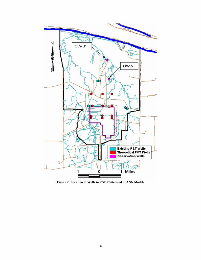
Figure 2: Location of Wells in PGDP Site used in ANN Models

4

1.3 MODEL DESCRIPTION

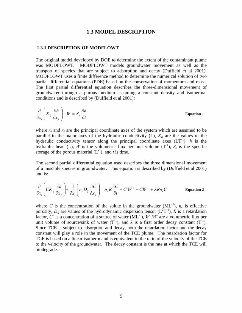
1.3.1 DESCRIPTION OF MODFLOWT The original model developed by DOE to determine the extent of the contaminant plume was MODFLOWT. MODFLOWT models groundwater movement as well as the transport of species that are subject to adsorption and decay (Duffield et al 2001). MODFLOWT uses a finite difference method to determine the numerical solution of two partial differential equations (PDE) based on the conservation of momentum and mass. The first partial differential equation describes the three-dimensional movement of groundwater through a porous medium assuming a constant density and isothermal conditions and is described by (Duffield et al 2001):

thSW

xhK

x sj

iji ∂

∂=−⎟

⎟⎠

⎞⎜⎜⎝

⎛

∂∂

∂∂

Equation 1

where xi and xj are the principal coordinate axes of the system which are assumed to be parallel to the major axes of the hydraulic conductivity (L), Kij are the values of the hydraulic conductivity tensor along the principal coordinate axes (LT-1), h is the hydraulic head (L), W is the volumetric flux per unit volume (T-1), Ss is the specific storage of the porous material (L-1), and t is time. The second partial differential equation used describes the three dimensional movement of a miscible species in groundwater. This equation is described by (Duffield et al 2001) and is:

CRnCWWCtCRn

xCDn

xxhCK

x eej

ijeij

iji

λ+−+∂∂

=⎟⎟⎠

⎞⎜⎜⎝

⎛

∂∂

∂∂

+⎟⎟⎠

⎞⎜⎜⎝

⎛

∂∂

∂∂ −+' Equation 2

where C is the concentration of the solute in the groundwater (ML-3), ne is effective porosity, Dij are values of the hydrodynamic dispersion tensor (L2T-1), R is a retardation factor, C’ is a concentration of a source of water (ML-3), W+/W- are a volumetric flux per unit volume of source/sink of water (T-1), and λ is a first order decay constant (T-1). Since TCE is subject to adsorption and decay, both the retardation factor and the decay constant will play a role in the movement of the TCE plume. The retardation factor for TCE is based on a linear isotherm and is equivalent to the ratio of the velocity of the TCE to the velocity of the groundwater. The decay constant is the rate at which the TCE will biodegrade.

5

1.3.2 THE FINITE DIFFERENCE METHOD As stated earlier, MODFLOWT uses a finite difference method to calculate head and constituent concentrations. The actual values of head and concentration are calculated by solving a system of simultaneous linear finite difference equations which are used to represent the PDEs. Figure 3 shows a typical setup for a 3-dimensional finite difference grid. The index i is the row indicator, j is the column indicator and k is the layer indicator. MODFLOWT uses a block-centered formulation in which the model solves for the value of the state variable at the center of the cell. For a more detailed description of the finite difference method used in MODFLOWT, please see Duffield et al (2001).

Figure 3: Three-Dimensional Finite Difference Grid

1.3.3 STRESS PERIODS MODFLOWT accommodates changes in system boundary conditions (e.g. different pumping rates, different source concentrations, etc.) through the use of different “stress periods.” A stress period is a user-defined length of time in which all conditions in the model remain constant. At the end of one stress period, a new stress period will begin using the new conditions, but the input data will be the output from the previous stress period. The MODFLOWT model used in this study contains two stress periods. The first stress period simulates the existing conditions at the PGDP site which is a pump and treat operation. This began in 1997 and continues until the present. The second stress period is used to simulate the new treatment process implemented into the model. The length of the second stress period varies depending on the particular model application. Within each stress period, state variables (such as groundwater elevation and constituent concentration) are determined at different time steps. Each time period is denoted by the number of days at which the calculations were performed. The total number of time

6

periods that are used is determined internally by MODFLOWT in order to ensure numerical stability when performing the associated finite difference calculations. It is typical to extract out results from a given number of years in the future (i.e. 50 years or 18,250 days). However, there may not be an exact time period of 18,250 days in MODFLOWT. In this case, the time period that was closest to the number of days of the future year was selected.

1.3.4 DESCRIPTION OF GROUNDWATER VISTAS

The software interface used to run MODFLOWT was Groundwater Vistas (GV). Groundwater Vistas is a model interface that incorporates multiple groundwater models into one software program. Through use of graphical analysis tools it is easy to setup, edit, and analyze model results. GV uses a mesh grid system which breaks the model into cells. A cell is a space in the finite difference grid that has consistent properties throughout and serves as a point of calculation. Each cell is located by a row, column, and layer number. All cells that have the same distinct set of properties are grouped into a zone. This feature gives the user the ability to adjust a parameter in all cells within a zone by use of a database option instead of changing each individual cell. The option to make changes cell by cell is also available. It also allows the user to see the model design in a plan and layout view. GV allows for easy editing of boundary conditions, soil properties, hydrologic properties and contaminant properties. GV allows the user to add multiple boundary conditions such as constant head/concentration, well, river, stream, no flow, wall or lake. Soil properties include hydraulic conductivity, porosity, initial contaminant concentrations, and diffusion. Hydrologic conditions are recharge and evapotranspiration. Contaminant properties are chemical reaction rates which includes the distribution coefficient, bulk density, and half-life. Since GV is model independent, users only need to learn the interface and not the actual models that it supports. The type of model used in GV can simply be changed by selecting the desired model from the Model menu and adding additional input if required. The version of GV used supports the following models: MODFLOW, MODPATH, MT3D, MODFLOWT, as well as a few others. For a more detailed description of GV refer to the user manual (Rumbaugh and Rumbaugh 2004).

1.4 MODEL VERIFICATION The baseline version of the MODFLOWT model was obtained from DOE. Previous study results from the model were compared to those obtained from previous DOE simulations. The model results were consistent with those of the DOE runs, thus validating the model (Lingireddy et al 2007).

7

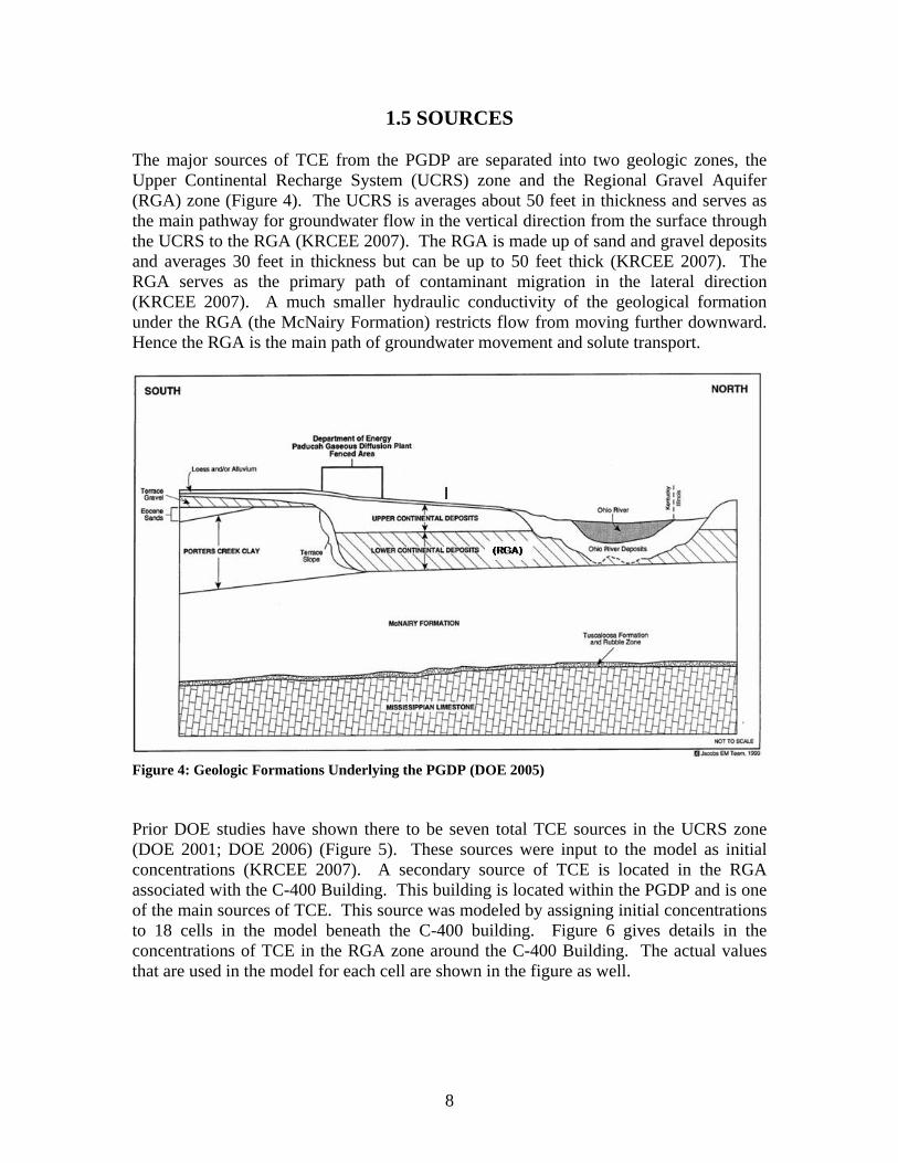
1.5 SOURCES The major sources of TCE from the PGDP are separated into two geologic zones, the Upper Continental Recharge System (UCRS) zone and the Regional Gravel Aquifer (RGA) zone (Figure 4). The UCRS is averages about 50 feet in thickness and serves as the main pathway for groundwater flow in the vertical direction from the surface through the UCRS to the RGA (KRCEE 2007). The RGA is made up of sand and gravel deposits and averages 30 feet in thickness but can be up to 50 feet thick (KRCEE 2007). The RGA serves as the primary path of contaminant migration in the lateral direction (KRCEE 2007). A much smaller hydraulic conductivity of the geological formation under the RGA (the McNairy Formation) restricts flow from moving further downward. Hence the RGA is the main path of groundwater movement and solute transport.

Figure 4: Geologic Formations Underlying the PGDP (DOE 2005) Prior DOE studies have shown there to be seven total TCE sources in the UCRS zone (DOE 2001; DOE 2006) (Figure 5). These sources were input to the model as initial concentrations (KRCEE 2007). A secondary source of TCE is located in the RGA associated with the C-400 Building. This building is located within the PGDP and is one of the main sources of TCE. This source was modeled by assigning initial concentrations to 18 cells in the model beneath the C-400 building. Figure 6 gives details in the concentrations of TCE in the RGA zone around the C-400 Building. The actual values that are used in the model for each cell are shown in the figure as well.

8

Figure 5: Location of the Seven Primary UCRS Sources

9

Figure 6: Spatial Distribution of Initial TCE Concentrations in the RGA Under the C400 Building

1.6 SUMMARY An alternative model that can be coupled with an optimization method will be developed based on artificial neural network technology. This model will serve as an alternative to MODFLOWT which models groundwater movement as well as contaminant transport for species subject to adsorption and decay. MODFLOWT has currently been used to model the movement of a TCE plume in the underlying aquifer of the Paducah Gaseous Diffusion Plant.

10

2.1 PURPOSE OF THE ARTIFICIAL NEURAL NETWORK The purpose of this particular artificial neural network model was to forecast TCE concentrations as accurately as the MODFLOWT model so that it can be incorporated with an optimization technique to form a management model. An optimization model requires numerous evaluations of the objective function and this is not feasible with a MODFLOWT model that can take hours for one simulation. A properly trained ANN model could give results of the objective function in seconds. In order for the ANN model applicable to this type of application, it must require less input and take less time to finish than the MODFLOWT model. Therefore, inputs will be limited to the pumping rates at the extraction wells used in the P&T process. Also, multiple ANN models with varying number of inputs will be developed to determine the optimal number of inputs. This will give the model that still produces satisfactory results yet requires the minimal number of inputs. Outputs will be TCE concentrations in two observations wells at four future times. These years will be 2009, 2015, 2021, and 2027.

2.2 ARTIFICIAL NEURAL NETWORKS Artificial neural networks are an inductive modeling technique used in many fields of research. ANNs are popularly applied in forecasting, pattern recognition, and classification problems. An ANN serves as an alternative to linear and non-linear regression and is very useful when the actual physical relationship between two or more variables is unknown. Each ANN model will be different and will depend on the data available to train with, the desired output, and the architecture of the model used. The architecture of the ANN model is dependent highly on the type of problem being considered (Maier and Dandy, 1999). Numerous studies have shown that the best setup for an ANN consists on one input, one hidden, and one output layer (see Figure 7). However this is not always the case, as some functions may prove to be difficult to approximate with one hidden layer thus requiring an additional layer of hidden nodes (Cheng and Titterington, 1994). The number of input nodes is fixed to the number of model inputs while the number of output nodes is fixed to the number of model outputs. The number of nodes in the hidden layer is critical since it will determine the number of connection weights (Maier and Dandy 1999). A supervised training approach was used for this study. Supervised training is where inputs and known outputs are required to perform the training of the model. During the training process the ANN determines the underlying causal relationship between the input and output data. The goal of the training process is to minimize the error between the observed and the predicted output of the model.

11

Figure 7: General ANN Model Architecture A feed-forward multi-layered perceptron (MLP) was used as the model architecture. In this architecture neurons are arranged in layers (see Figure 7). Input layer neurons are buffers that normalize the incoming data. For this study normalization was based on the greatest value of the input data resulting in values that ranged from 0 to 1. The hidden layer and output layer neurons are defined as activation functions. An activation function will transform the input and pass it to the subsequent layer and will be discussed in greater detail in a later section. The result of the output neuron will be the output of the model to the user. Neurons in different layers are interconnected by weights (see Figure 7). The information is passed from left to right (i.e. input to hidden layer, hidden to output layer). The trained knowledge of the model is stored in these weights. Equation 3 shows how the trained knowledge of the weights as it is applied to the inputs.

j

n

iii netwx =∑

=11 Equation 3

where xi is the input from the ith neuron in the preceding layer and w1i is the weight interconnecting the ith neuron in the preceding layer to neuron 1 in the hidden layer (see Figure 7). The netj term is the weighted sum and this information is then transformed by the activation function as shown in Equation 4.

( )jnetj enetf

λ−+=

11)( Equation 4

where λ is a learning rate that determines how much the function will transform. The interconnecting weights are redefined by the training algorithm and represent the knowledge gained by the ANN model. A new set of inputs can then be used and the process repeated.

12

2.1.1 TRAINING, TESTING, AND VALIDATION The more datasets that are available to train and validate the model, the more accurate the model will be. After training has finished a model needs to be validated to ensure that it is a robust model and that it is not over training the data. Validation needs to occur with a separate group of datasets that has not been used in training or testing process (Maier and Dandy 1999). Caution needs to be taken to prevent memorization of the training datasets which will result in an inadequate model. Memorization of data describes the condition whereby too many connection weights have allowed overtraining of the data, which is where the model has learned the idiosyncrasies of the training set, thus the model loses its ability to generalize (Maier and Dandy 1999). When memorization occurs, the model has been over-trained and has captured noise from the dataset. The most standard way to prevent this from occurring is to divide the datasets into three sub-sets: a training set, a testing set, and a validation set. Literature typically suggests division of data into training/testing and validation of 80% vs. 20% or 70% vs. 30% (Maier and Dandy 1999). The training and testing data is then further divided by the same percentage as the previous division. Each sub-set of data must be representative of the entire dataset to ensure good training (Maier and Dandy 1999). The training set is used to train the ANN model. The testing set should not be used in training so that the data is new to the model. It can then be simulated in the model and the error results from training and testing can be compared. If the training and testing errors are significantly different, then memorization most probably took place during training and a better model will need to be developed. Memorization of the model can be detected by a continual reduction in the training set error while the testing set error remains the same or becomes worse (Maier and Dandy 1999).

2.1.2 ACTIVATION FUNCTIONS Types of activation functions commonly used are logistic sigmoid (unipolar activation) with an output variation of 0 to 1, hyperbolic tangent sigmoid (bipolar activation) with an output variation of -1 to 1, and linear that only has values of 0 and 1. Maier and Dandy (1999) found that other activation functions may be used as long as they are differentiable. Normalization of the data must take place to ensure that values of netj stay with the range of the function. The unipolar activation function was used for the ANN models in this study. The graph of this function is shown in Figure 8.

13

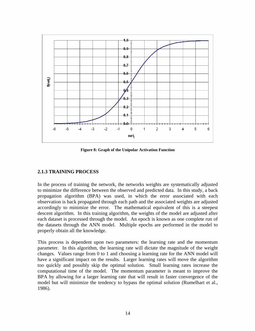
Figure 8: Graph of the Unipolar Activation Function

2.1.3 TRAINING PROCESS In the process of training the network, the networks weights are systematically adjusted to minimize the difference between the observed and predicted data. In this study, a back propagation algorithm (BPA) was used, in which the error associated with each observation is back propagated through each path and the associated weights are adjusted accordingly to minimize the error. The mathematical equivalent of this is a steepest descent algorithm. In this training algorithm, the weights of the model are adjusted after each dataset is processed through the model. An epoch is known as one complete run of the datasets through the ANN model. Multiple epochs are performed in the model to properly obtain all the knowledge. This process is dependent upon two parameters: the learning rate and the momentum parameter. In this algorithm, the learning rate will dictate the magnitude of the weight changes. Values range from 0 to 1 and choosing a learning rate for the ANN model will have a significant impact on the results. Larger learning rates will move the algorithm too quickly and possibly skip the optimal solution. Small learning rates increase the computational time of the model. The momentum parameter is meant to improve the BPA by allowing for a larger learning rate that will result in faster convergence of the model but will minimize the tendency to bypass the optimal solution (Rumelhart et al., 1986).

14

2.5 ANN MODELING SOFTWARE The ANN training and simulation was done by using Neurosort 3.0, a neural network software program specially designed for water and environmental engineering. Neurosort 3.0 was developed at the University of Kentucky and has been successfully applied to numerous applications. It allows the user to change parameters and model architecture with an easy to use graphic interface.

2.3 DATASETS The datasets for the ANN model were generated using the MODFLOWT model by adjusting the pumping rates of the extraction wells. As of now, the PGDP site has six existing extraction wells working in the pump and treat process. Twelve new theoretical extraction wells were added to the system to test the impact of future expansion of the pump and treat. (See Figure 2). The locations of these wells were selected so that they would cover the area of the initial TCE plume and remain near the PGDP boundary. All extraction wells are located in the third layer of the model. Forty-four MODFLOWT model runs were made with different pumping rates so there are 44 datasets to use in the ANN model.

2.3.1 INPUTS There were eighteen inputs available to design the ANN models. However, one of the goals of the ANN model is to minimize the number of inputs required. Therefore a correlation analysis was made between the pumping rates at each extraction well and the TCE concentration extracted from MODFLOWT at each observation well. The initial ANN model developed used all eighteen available inputs. This gave a baseline values to compare the other models against. The second model consisted of fifteen inputs. For additional ANN models, the two lowest correlating extraction wells were removed. The minimum number of inputs to any ANN was five. This process was done for two observation wells. Table 1 shows the specific extraction wells that were used in each ANN model.

15

Table 1: Extraction Wells used in ANN Models Created to Determine Optimal Number of Inputs Observatio Well Bayou-1

1 2 3 4 5 6 7 8 9 10 11 12 13 14 15 16 17 1818 Wells X X X X X X X X X X X X X X X X X X15 Wells X X X X X X X X X X X X X X X13 Wells X X X X X X X X X X X X X11 Wells X X X X X X X X X X X9 Wells X X X X X X X X X7 Wells X X X X X X X5 Wells X X X X X

1 2 3 4 5 6 7 8 9 10 11 12 13 14 15 16 17 1818 Wells X X X X X X X X X X X X X X X X X X15 Wells X X X X X X X X X X X X X X X13 Wells X X X X X X X X X X X X X11 Wells X X X X X X X X X X X9 Wells X X X X X X X X X7 Wells X X X X X X X5 Wells X X X X X

Num

ber o

f AN

N

Inpu

ts

Extraction Well

Num

ber o

f AN

N

Inpu

ts

Observation Well 5Extraction Well

2.3.2 OUTPUTS The ANN outputs were TCE concentrations in observation wells located inside the water policy boundary. Currently there are 14 observation wells inside the water policy boundary. Fifteen theoretical observation wells were added and placed such that they would cover representative sections inside the boundary. The four outputs of the models will be concentrations at 2009, 2015, 2021, and 2027. Initially ten observation wells were chosen throughout the PGDP site. To limit the extent of this project, only two observation wells were analyzed. Both these wells had significant change in concentrations with change in the pumping rates so they are a good indicator of the ANN model potential. Observation well Bayou-1 (OW-B1) and Observation Well 5 (OW-5) were the two selected. OW-B1 is an existing observation well and OW-5 is a theoretical observation well to the model

2.3.3 SIMULATIONS A total of 44 pumping simulations were run using MODFLOWT resulting in 44 datasets to be used in training and validation of the ANN model (Table 2). Each simulation consisted of only the theoretical wells, only the existing wells, or a combination of the both. The pumping rates for the existing extraction wells are shown in Table 3. The pumping rates for the theoretical extraction wells were chosen to be 0, 50, or 100 gpm. These values are a good representation of the pumping rates of the existing extraction wells used in the P&T process.

16

The 44 datasets were randomly sorted before being broken down into the training/testing and validation sets. This will prevent the model from being over calibrated. From this randomized list of datasets, 26 sets were used for training, 9 sets for testing, and 9 sets for validation.

17

Table 2: Pumping Simulations for each Dataset

Simulation 1 2 3 4 5 6 7 8 9 10 11 12 13 14 15 16 17 181 100 100 100 100 100 100 100 100 100 100 100 100 0 0 0 0 0 02 50 50 50 50 50 50 50 50 50 50 50 50 0 0 0 0 0 03 0 0 0 100 100 100 100 100 100 100 100 100 0 0 0 0 0 04 100 100 100 0 0 0 100 100 100 100 100 100 0 0 0 0 0 05 100 100 100 100 100 100 0 0 0 100 100 100 0 0 0 0 0 06 100 100 100 100 100 100 100 100 100 0 0 0 0 0 0 0 0 07 0 0 0 50 50 50 50 50 50 50 50 50 0 0 0 0 0 08 50 50 50 0 0 0 50 50 50 50 50 50 0 0 0 0 0 09 50 50 50 50 50 50 0 0 0 50 50 50 0 0 0 0 0 0

10 50 50 50 50 50 50 50 50 50 0 0 0 0 0 0 0 0 011 0 100 100 0 100 100 0 100 100 0 100 100 0 0 0 0 0 012 100 0 100 100 0 100 100 0 100 100 0 100 0 0 0 0 0 013 100 100 0 100 100 0 100 100 0 100 100 0 0 0 0 0 0 014 0 50 50 0 50 50 0 50 50 0 50 50 0 0 0 0 0 015 50 0 50 50 0 50 50 0 50 50 0 50 0 0 0 0 0 016 50 50 0 50 50 0 50 50 0 50 50 0 0 0 0 0 0 017 100 100 100 100 100 100 50 50 50 50 50 50 0 0 0 0 0 018 100 100 100 50 50 50 100 100 100 50 50 50 0 0 0 0 0 019 100 100 100 50 50 50 50 50 50 100 100 100 0 0 0 0 0 020 50 50 50 100 100 100 100 100 100 50 50 50 0 0 0 0 0 021 50 50 50 100 100 100 100 50 50 100 100 100 0 0 0 0 0 022 50 50 50 50 50 50 100 100 100 100 100 100 0 0 0 0 0 023 100 100 50 100 100 50 100 100 50 100 100 50 0 0 0 0 0 024 100 50 100 100 50 100 100 50 100 100 50 100 0 0 0 0 0 025 50 100 100 50 100 100 50 100 100 50 100 100 0 0 0 0 0 026 100 50 50 100 50 50 100 50 50 100 50 50 0 0 0 0 0 027 50 100 50 50 100 50 50 100 50 50 100 50 0 0 0 0 0 028 50 50 100 50 50 100 50 50 100 50 50 100 0 0 0 0 0 029 100 0 100 0 100 0 0 100 0 100 0 100 0 0 0 0 0 030 50 0 50 0 50 0 0 50 0 50 0 50 0 0 0 0 0 031 100 100 100 100 100 100 100 100 100 100 100 100 48 45 60 55 100 8032 50 50 50 50 50 50 50 50 50 50 50 50 48 45 60 55 100 8033 0 0 0 0 0 0 0 0 0 0 0 0 48 45 60 55 100 8034 100 100 100 100 100 100 100 100 100 100 100 100 48 45 60 55 0 035 100 100 100 100 100 100 100 100 100 100 100 100 48 45 0 0 100 8036 50 50 50 50 50 50 50 50 50 50 50 50 0 0 60 55 100 8037 0 0 0 0 0 0 0 0 0 0 0 0 100 100 100 100 100 10038 0 0 0 0 0 0 0 0 0 0 0 0 50 50 50 50 50 5039 0 0 0 0 0 0 0 0 0 0 0 0 50 100 50 100 50 10040 0 0 0 0 0 0 0 0 0 0 0 0 50 50 100 100 50 5041 0 0 0 0 0 0 0 0 0 0 0 0 100 100 50 50 100 10042 0 0 100 0 0 100 0 100 0 100 0 0 48 45 60 55 100 8043 0 0 100 0 0 100 0 100 0 100 0 0 100 100 100 100 100 10044 0 0 100 0 0 100 0 100 0 100 0 0 50 50 50 50 50 50

Theoretical Extraction Wells (gpm) Existing Extraction Wells (gpm)

18

Table 3: Pumping Rates at Existing Extraction Wells (KRCEE 2007)

Extraction Well Existing Pumping Rate (gpm)Well 13 48Well 14 45Well 15 60Well 16 55Well 17 100Well 18 80

Each MODFLOWT model run consisted of two stress periods. The first stress period consisted of 10 years starting in 1997 in which there was no pumping in any wells (theoretical or existing). The second stress period started in 2007 and consisted of 20 years in which the pumping simulations were active the entire time.

2.4 ARCHITECHTURE USED For the solute transport problem, the architecture and parameters used are shown in Figure 9 and Table 4 respectively. The Neurosort software also requires that an initial set of weights selected and the total number of iterations be specified. Neurosort offers ten default initial weights sets to choose from. The initial weight set chosen was set 1 and number of iterations was 10000. This setup and parameter listing were determined by a trial and error procedure.

Figure 9: Artificial Neural Network (shown with 18 inputs) for One Observation Well

19

Table 4: ANN Parameter Values

ParameterHidden Nodes 3Training/Testing 3/1Learning Rate 0.1Momentum Parameter 0.4

2.6 RESULTS An ANN model was created for each number of inputs given in Table 1. The accuracy of each ANN model was assessed based on the coefficient of determination value (R2 value) of the predicted versus observed concentrations. Table 5 shows the R2 values of each ANN model for both observation wells. The R2 value is an average of all four output years for both the training and validation set. R2 is based on Equation 5.

( )

( ) ( )∑ ∑

∑

= =

=

−+−

−−= n

i

n

iiii

n

iii

oppo

opR

1 1

22

1

2

2 1 Equation 5

where p is the predicted outputs by the ANN model and o is the observed outputs from the MODFLOWT model. Each ANN model is labeled by the observation well (i.e. OW-B1) and then by the number of inputs for that particular model (i.e. 5 for five inputs). Based on the R2 values for the validation simulations it can be seen that for OW-B1, model OWB1-15 performed the best and for OW-5, model OW5-18 performed the best. The forecasted TCE concentrations for the validation simulations from these two models are the results presented here. These are shown in Figure 10 for OW-B1 and Figure 11 for OW-5.

Table 5: R2 Values from ANN Models for Observation Wells Bayou-1 and 5

Model NameNumber of

Inputs R2 Model NameNumber of

Inputs R2

OWB1-18 18 0.8944 OW5-18 18 0.9060OWB1-15 15 0.9095 OW5-15 15 0.8820OWB1-13 13 0.9065 OW5-13 13 0.8179OWB1-11 11 0.8830 OW5-11 11 0.8207OWB1-9 9 0.7938 OW5-9 9 0.8155OWB1-7 7 0.7618 OW5-7 7 0.5947OWB1-5 5 0.1182 OW5-5 5 0.5977

O.W. 5O.W. Bayou-1

20

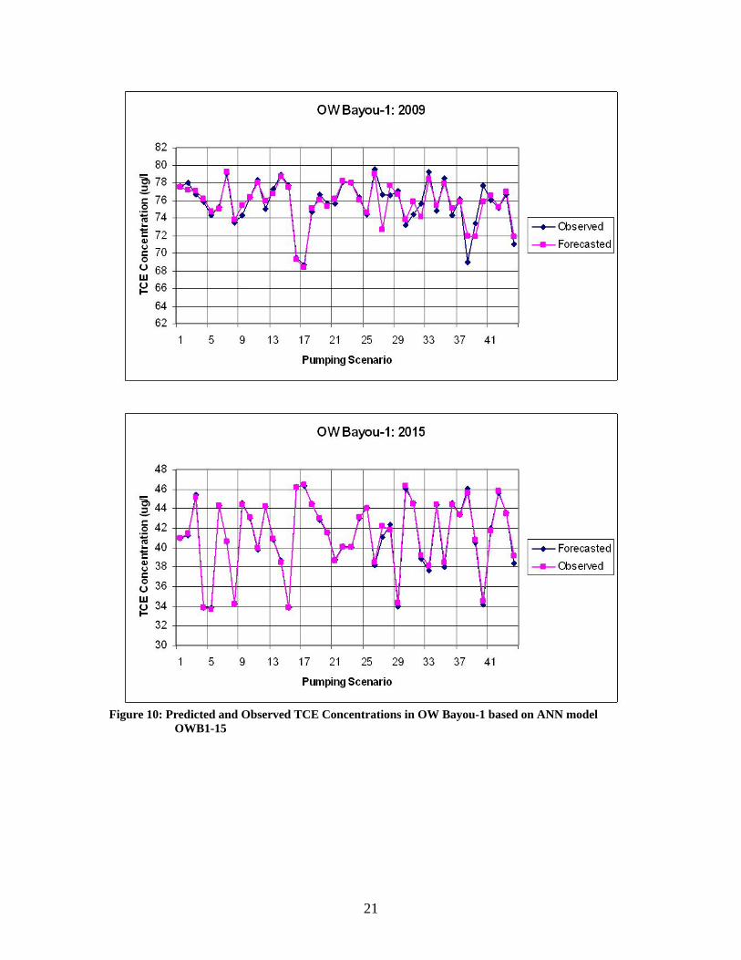
Figure 10: Predicted and Observed TCE Concentrations in OW Bayou-1 based on ANN model

OWB1-15

21

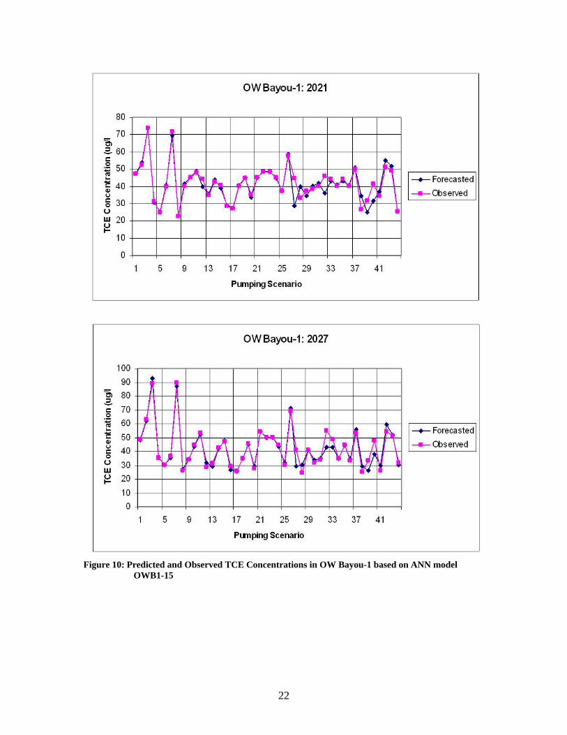
Figure 10: Predicted and Observed TCE Concentrations in OW Bayou-1 based on ANN model

OWB1-15

22

Figure 11: Predicted and Observed TCE Concentrations in OW 5 based on ANN model OW5-15

23

Figure 11: Predicted and Observed TCE Concentrations in OW 5 based on ANN model OW5-15

24

2.7 DISCUSSION

Based on the R2 values for the particular year, both models performed well in predicting the TCE concentrations at their respective observation wells. With the exception of a few outliers, it appears that the observed and predicted data was a good match. Table 6 give the individual R2 values for the ANN models presented.

Table 6: R2 Values from ANN Models for Individual Years

OWB1 OW52009 0.8391 0.97752015 0.9943 0.97522021 0.8674 0.86992027 0.9371 0.8016

Observation WellYear

From Table 5, it can be seen that by dropping a substantial number of inputs a model with an acceptable R2 value could still be created. Both models could have only nine inputs and still produce an R2 of approximately 0.80. Figures 12 and 13 show scatter plots of observed versus predicted output data for both observation wells. Based on these scatter plots, neither model appears to be biased since the deviation of residuals is fairly uniformed distributed about a 45º. The models are not exact when forecasting the concentrations, but they are accurate enough to help in identifying potentially impacted properties. If the extraction well locations are known and pumping rates remain constant, an ANN model could help determine areas of possible health risk.

2.7.1 LIMITATIONS The developed ANN has some limitations. Since the wells used as input (extraction) and output (observation) did not change position, the ANN model will only be valid for wells in these same locations. Hence if 18 different extraction wells were used at different geographic locations, a new ANN would need to be developed. However, once a well location has been determined, it can be considered permanent since it is unlikely that they will be moved from one place to another. Thus, an ANN could be developed once these permanent locations are known. The ANN is also only valid for the observation well from which the training data came. So if there are five observations wells, five different ANN models would need to be developed. Multiple observations wells were attempted in one ANN model, but did not give satisfactory results. This model does not reflect on changes to the physical characteristics of the area of study. Changes in recharge, leakage, source concentrations etc. would require additional inputs to the model. For this model development, these parameters were not considered because

25

they remained constant for all the MODFLOWT runs which were used for data generation. These parameters were calculated in the MODFLOWT model based on vast field experimentations. Again, for the purpose of this report the model inputs were limited strictly to the pumping rates of the extraction wells. Another limitation to this model is that the pumping rates in the extraction wells were set at a few specific values. In reality, the likelihood of all wells pumping at one of these specific rates is not very likely. Each well would have its own specific rate depending on its size and aquifer properties at that location such as hydraulic conductivity, storage coefficient, etc.

2.7.2 FUTURE INVESTIGATIONS One area to further investigate is to develop a more general ANN model by incorporating different locations of wells. This type of model could help in determining the best placement of an extraction well, which would minimize the extent of the contaminant plume. An extension of this would be to incorporate these ANNs with an optimization technique to optimize the pumping strategy to reduce concentrations at a point in the study area to an acceptable concentration.

26

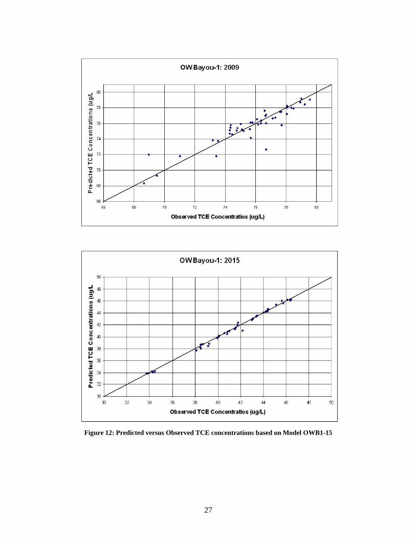
Figure 12: Predicted versus Observed TCE concentrations based on Model OWB1-15

27

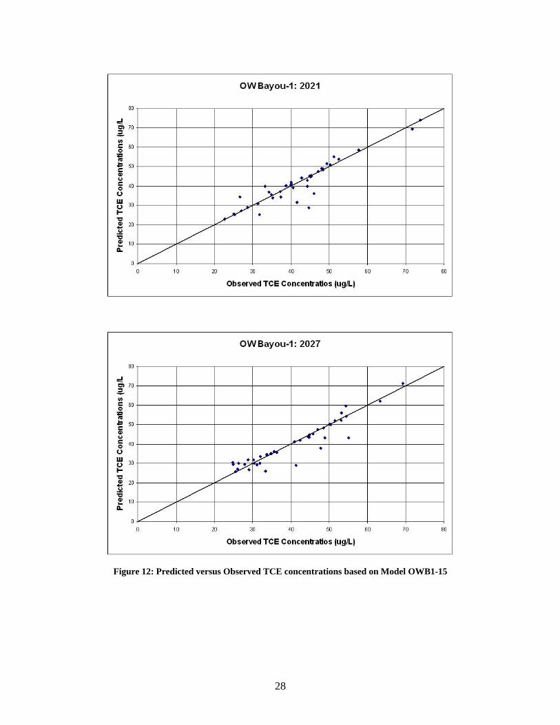
Figure 12: Predicted versus Observed TCE concentrations based on Model OWB1-15

28

Figure 13: Predicted versus Observed TCE concentrations based on Model OW5-18

29

Figure 143: Predicted versus Observed TCE concentrations based on Model OW5-18

30

WORKS CITED ATSDR, 2007. Retrieved from (http://www.atsdr.cdc.gov/tfacts19.html#bookmark03).

Retrieved on 4/11/07. ATSDR, 2001. Public Health Assessment, Paducah Gaseous Diffusion Plant, retrieved

from (http://www.atsdr.cdc.gov/HAC/PHA/paducah/pad_toc.html). Retrieved on 4/11/07.

Cheng. B., and Titterington, D.M. 1994. Neural Networks: A review from a statistical

perspective. Statistical Science 9 (1). 2-54. DOE (U.S. Department of Energy) 2001. Feasibility Study for the Groundwater Operable

Unit at Paducah Gaseous Diffusion Plant, Paducah, Kentucky – Volume 4. Appendix C Supporting Information for Feasibility Study, DOE/OR/07-1857&D2, Bechtel Jacobs Company, LLC, Oak Ridge, TN.

DOE (U. S. Department of Energy) 2005. Trichloroethene and Technetium-99

Groundwater Contamination in the Regional Gravel Aquifer for Calendar Year 2004 at the Paducah Gaseous Diffusion Plant, Paducah, Kentucky, JJC/PAD-169/R5 Final, Bechtel Jacobs Company, LLC, Paducah, KY, July.

DOE (U.S. Department of Energy) 2006. Site Investigation Report for the Southwest

Groundwater Plume at the Paducah Gaseous Diffusion Plant, Paducah, Kentucky, DOE/OR/07-2180&D2, Paducah Remediation Services, LLC, Paducah, Kentucky.

Duffield, G.M., Benegar, J.J., and Ward, D.S. 2001. MODFLOWT: A Modular Three-

Dimensional Groundwater Flow and Transport Model. HydroSOLVE Inc. and HIS GeoTrans. Sterling, VA.

Ensley, B.D. 1991. Biochemical Diversity of Trichloroethylene Metabolism. Annu. Rev.

Microbiol. (45) 283-99. EPA 2007. Superfund Frequently Asked Questions, retrieved from

(http://www.epa.gov/superfund/contacts/index.htm). Retrieved on 4/11/07. KRCEE (Kentucky Research Consortium for Energy and Environment). 2007. Property

Acquisition Study for Areas near the Paducah Gaseous Diffusion Plant, Paducah, Kentucky

Lingireddy, S., Viswanathan, C., and Hampson S. (2007) “Evaluation of Paducah

Gaseous Diffusion Plant Groundwater Flow and Contaminant Transport Model.” KRCEE.

31

Maier, H.R., and Dandy, C.D. 1999. “Neural networks for the prediction and forecasting of water resources variables: a review of modeling issues and applications.” Environmental and Modelling Software. 15, 101-124.

Rumbaugh, J.O. and Rumbaugh, D.B. 2004. Groundwater Vistas Guide to Using,

Version 4. Environmental Simulations, Inc. Reinholds, PA. Rumelhart, D.E., Hinton, G.E., Williams, R.J., 1986. “Learning internal representation

by back- propagating errors.” In: Rumelhart, D.E., McCleland, J.L., the PDP Research Group (Eds.), Parallel Distributed Processing: Explorations in the Microstructure of Cognition. MIT Press, MA.

32