Sensititity of the stability threshold in linearizedrotordynamics

B.Vervisch 1,2,K.Stockman 1,2, M.Loccufier 2

1 Technical University of West-Flanders, Department of Electromechanical Engineering,Graaf Karel de Goedelaan 5, B-8500, Kortrijk, Belgiume-mail: bram.vervisch@howest.be

2 University of Ghent, Departement of Electrical Engineering, Systems and AutomationTechnologiepark 914, B-9052, Zwijnaarde, Belgium

AbstractRotors exposed to lateral vibration can become unstable at a certain speed due to rotor internal damping.This stability threshold speed is unique and it is impossible to rotate above the threshold. In this paper,a rotor is treated as a linear speed dependent system and inertia, stiffness, gyroscopic and damping forcesare included. In order to find the stability threshold, the multiple degree of freedom equations of motionare decoupled into a set of scalar equations. Therefore, the quadratic eigenvalue problem has to be solved.Consequently, the stability threshold speed can be calculated as the lowest speed by which one of the rootshas a positive real part. The parameters that influence this stability threshold are discussed and verified bynumerical results.

1 Introduction

Self-excited vibrations have been a field of study in linearized rotordynamics, for over a century. Ever sinceDe Laval proved experimentally in 1895 that turbines can operate supercritically, in order to increase per-formance for lower dimensions, manufacturers became aware of severe vibrations and instabilities whenoperating at this speed. Nowadays, high speed, high performance and reliable rotating machinery play animportant role in many industries going from power generation to manufacturing and even home appliances[1]. To satisfy all these expectations, an accurate knowledge of the stability threshold is required. Besides thewidely known oil whirl and whip phenomenon induced by hydrodynamic bearings, rotor internal damping isrecognized as one of the main causes of self-excited vibrations [2]. This type of damping induces a followerforce, increasing the whirling amplitude in the supercritical field. It is shown theoretically that the whirlingmotion of the rotor becomes unstable at all speeds above the stability threshold and that this threshold is al-ways larger than the corresponding whirling speed [3]. However, the stability threshold is highly dependenton the model structure and in order to get a realistic estimation, the model should include all the forces thataffect this threshold. These are typically inertia, stiffness, gyroscopic and damping forces. On the contrary,in the industry, a model should be as simplified as possible to gain insight and to reduce computational time.Therefore a model that is linear and time invariant for a fixed speed is preferred in rotordynamics. This typeof model is usually the result of a discretization technique such as finite elements [4].In this paper, the sensitivity of the stability threshold is studied for these kinds of models. Therefore, thequadratic eigenvalue problem is solved[5]. Because of the impossibility to rotate above the stability thresh-old, the actual threshold will be the one with the lowest speed. It is widely known that for an undampednon-rotating system, the eigenvalues and their corresponding eigenvectors have a specific ordering which ischaracterized by Rayleigh’s coefficient. As long as the system has specific properties, a similar techniquecan be used to study the effect of the eigenvectors on the stability threshold. Otherwise, only experimental

validation can give a solution.In section two, the equations of motion for the linear speed dependent model and the choice for complex co-ordinates are explained. Subsequently, section three discusses the matrices of the finite element model with aspecial focus on the damping matrix containing either viscous damping, hysteretic damping or a combinationof both. Taking this into account, the stability threshold speed is calculated for a system that is uncoupled byits eigenvectors in section four. With this method, the stability threshold speed is defined by five parameters.These parameters can also lead to a Campbell diagram and a decay rate plot. In a similar way, the ordering ofthe stability threshold is questioned. Finally, in section five, the theory is illustrated with numerical results.

2 Equations of motion

2.1 The linear speed dependent model

Whereas rotating structures are generally nonlinear and continuous, this kind of system is mostly linearizedand discretized. However, this linearization is only valid under the assumption that the vibrations are smalland the accuracy of the discretization technique will only be sufficient if enough elements are chosen; awidely used concept. As a result, typical equations of motion are obtained containing a mass matrix, M,a damping matrix, C, and stiffness matrix, K. However, due to rotation, some of the properties changeperiodically in time, thus, the matrices become time dependent [6].

M(t)q + C(t)q + K(t)q = f(t), q(t), f(t) ∈ Rn (1)

with n, the degrees of freedom. In most rotating machinery, the structure is commonly assumed to containonly isotropic rotating elements with properties invarient in time. Under these assumptions, the matrixproperties are no longer time depentent, but only speed dependent and equation (1) can be simplified:

M(Ω)q + C(Ω)q + K(Ω)q = f(t), q(t), f ∈ Rn (2)

with Ω the rotating speed. In non-rotating structures, the mass matrix and the stiffness matrix representrespectively the conservative inertial and stiffness forces, while the damping matrix represents the non-conservative damping forces. In rotating structures these properties are mixed resulting in a combination ofconservative and non-conservative forces in both the damping and stiffness matrix [1]. For this reason thematrix C is sometimes called the velocity dependent matrix and K, the displacement dependent matrix [7].This terminology is used throughout this paper.

2.2 Complex coordinates

Independent of the discretization technique for a fixed rotation axis, every discrete node in the rotating systemhas four degrees of freedom: two translations (vi,wi) and two rotations (φyi, φzi) (Figure 1). Whenever therotor is axi-symmetrical, complex coordinates can be used [3].

qi =

[riφi

]=

[vi + iwiφyi − iφzi

]i =√−1 (3)

The use of complex coordinates is very expedient in axi-symmetrical systems. It allows to study the systemusing a model whose size is just half the size of the same problem expressed in real coordinates[4]. Therefore,complex coordinates will be used in the remainder of the paper.

x

yz

vi

wi

ϕxi

ϕyi

Figure 1: Schematic representation of the shaft on bearings divided in finite elements with four degrees offreedom per node

3 Discussion of the matrices

Mass, stiffness and gyroscopic matrices are usually derived from the kinetic and potential energy expression.Depending on the model resolution accuracy a lumped, distributed or consistent mass discretization can beused, whereas the consistent mass matrix appears to be slightly better for most cases [8]. The modelingof damping is not so straightforward. Usually, proportional damping is used which results in a viscousbehaviour. Otherwise hysteretic damping can be incorporated using complex stiffness. A combination ofboth is also possible.

3.1 Mass, stiffness and gyroscopic matrices

For the modeling of the mass, stiffness and gyroscopic matrices, a finite element model is used based on theEuler-Bernouilli beam theory. This means that the shear deformation is not taken into account. It has twonodes at both ends of the beam and six degrees of freedom per node. Because only lateral vibrations areconsidered, the degrees of freedom reduce to four. This matrices result in

Kel =EI

l3

12 6l −12 6l

4l2 −6l 2l2

12 −6lsymm 4l2

(4)

MTel =ρAl

420

156 l22 54 −13l

4l2 l13 −3l2

156 −22lsymm 4l2

(5)

MRel =ρI

30l

36 l3 36 −3l

4l2 l3 −1l2

36 −3lsymm 4l2

(6)

and

Mel = MTel + MRel, Gel = 2MRel (7)

With Kel, MTel and MRel respectively the stiffness, translational mass and rotational mass matrix. Mel andGel are the mass and the gyroscopic matrix. The stiffness of the bearings is taken into account as linearsprings on the nodes affecting both translation and rotation (Figure 1).

3.2 Damping matrices

3.2.1 Viscous damping

The damping matrices can be modeled in a proportional way if purely viscous damping is assumed. Propor-tional damping is defined as

Cn0 = aKb0 + bM (8)

Cr0 = aKr0 + bM (9)

with Kb0 containing the stiffness of the bearings and Kr0 the stiffness of the shaft. Usually, however, adamping coefficient is used to define the damping[9][3]. This both leads to matrices proportional to thestiffness matrix only.

Cn0 = ηbKb0 (10)

Cr0 = ηvKr0 (11)

with ηb and ηv the viscous loss factor for the bearings and the shaft. Because the shaft is rotating, the viscousdamping Cr0 acts in both the nonrotating and rotating frame. This results in both an influence in the velocitydependent matrix C(Ω) and the displacement dependent matrix K(Ω). Moreover, the latter introduces arotating speed dependency of the form ΩCr0.Viscous damping is easy to use but does not really have a physical interpretation. Therefore, hystereticdamping can be used as an alternative.

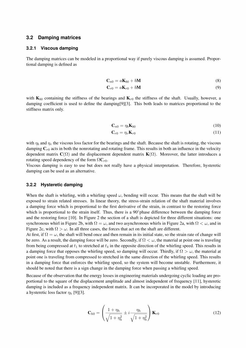
3.2.2 Hysteretic damping

When the shaft is whirling, with a whirling speed ω, bending will occur. This means that the shaft will beexposed to strain related stresses. In linear theory, the stress-strain relation of the shaft material involvesa damping force which is proportional to the first derivative of the strain, in contrast to the restoring forcewhich is proportional to the strain itself. Thus, there is a 90phase difference between the damping forceand the restoring force [10]. In Figure 2 the section of a shaft is depicted for three different situations: onesynchronous whirl in Figure 2b, with Ω = ω, and two asynchronous whirls in Figure 2a, with Ω < ω, and inFigure 2c, with Ω > ω. In all three cases, the forces that act on the shaft are different.At first, if Ω = ω, the shaft will bend once and then remain in its initial state, so the strain rate of change willbe zero. As a result, the damping force will be zero. Secondly, if Ω < ω, the material at point one is travelingfrom being compressed at t1 to stretched at t4 in the opposite direction of the whirling speed. This results ina damping force that opposes the whirling speed, so damping will occur. Thirdly, if Ω > ω, the material atpoint one is traveling from compressed to stretched in the same direction of the whirling speed. This resultsin a damping force that enforces the whirling speed, so the system will become unstable. Furthermore, itshould be noted that there is a sign change in the damping force when passing a whirling speed.

Because of the observation that the energy losses in engineering materials undergoing cyclic loading are pro-portional to the square of the displacement amplitude and almost independent of frequency [11], hystereticdamping is included as a frequency independent matrix. It can be incorporated in the model by introducinga hysteretic loss factor ηh [9][3].

Ch0 =

1 + ηh√1 + η2h

± i ηh√1 + η2h

Kr0 (12)

1

2

3

4

1

23

4

1

2

3

4

12

3 4

Ω

ω

Ω<ω

y

xz t1

t2

t3

t4

Ω

ω

Fd

Fr w

c(a) Rotating speed < whirling speed

Ω=ω

Ω

ω

Fr w

c

1

2

3

4

1

2

3

4

1

2

3

4

1

23

4

Ω

ω

y

xz t1

t2

t3

t4

(b) Rotating speed = speed

Ω>ω

Fd Ω

ω

Fr w

c

1

2

3

4

1

23

4

1

2

3

4

1 2

34

Ω

ω

y

xz t1

t2

t3

t4

(c) Rotating speed > whirling speed

Figure 2: Section of a shaft that is exposed to whirling

Because η2h << 1 this can be approximated by

Ch0 = (1 + ηh ± iηh) Kr0 (13)

The sign change of the imaginary part depends on the rotating speed, as explained above. Because of thecomplex coordinates, it is negative when Ω < ω and positive when Ω > ω.The disadvantage of this type of modeling is that it can only be used in systems with harmonic motion.

3.3 System equations

By the modeling choice explained above, equation (2) becomes

Mq + (ηbKb0 + ηvKr0 − iΩG0) q +

Kr0 + Kb0 + ηhKr0︸ ︷︷ ︸K0

−i (Ωηv ± ηh) Kr0

q = 0 (14)

where q is an n-dimensional vector containing the generalized coordinates [4]. This model includes inertial,stiffness, gyroscopic and damping forces. Centrifugal stiffening is neglected, the rotor is balanced and noexternal forces are observed. M represents the mass matrix, Kr0 and Kb0 the stiffness matrix of respectivelythe shaft and the bearings. The gyroscopic matrix, G0, represents the gyroscopic forces. Due to the complex

coordinates, all matrices are considered to be symmetric. In order to simplify further derivations, (14) isrewritten as

Mq + (Cn0 + Cr0 − iΩG0) q + [K0 − i (ΩCr0 ± Ch0)] q = 0 (15)

4 The stability threshold

4.1 Stability threshold speed

For the system in (18) a nonsingular linear transformation y = Tq exists such that it can be rewritten asfollows [12]:

y + (Cn0 + Cr0 − iΩG) y + [K0 − i (ΩCr0 ± Ch0)] y = 0 (16)

where K = diag(λ1, λ2, ..., λn) are the roots of the equation

det(Mλ−K0) = 0 (17)

If y = ueµt is a solution of the equation, a quadratic eigenvalue problem is formed

µ2 + (Cn + Cr − iΩG)µ+ [K− i (ΩCr ± Ch)]

u = 0 (18)

The solution of this problem gives rise to 4n eigenvalues µi and their corresponding eigenvectors ui. Theeigenvalues are of the form

µ = σ + iω (19)

where σ is the damping coefficient or the decay rate, and ω is the damped natural frequency. If equation (18)is premultiplied by its complex conjugate eigenvector uT , a scalar equation is obtained [3][1]

µ2 + (cn + cr − iΩg)µ+ k − i (Ωcr ± ch) = 0 (20)

The vector u, defined by an arbitrary constant, is chosen such that u∗u = 1. Due to the matrix properties thescalars cn, cr, g, ch and k are all real and positive and defined by

u∗Ku = k > 0 (21)

u∗Cru = cr ≥ 0 (22)

u∗Chu = ch ≥ 0 (23)

u∗Cnu = cn ≥ 0 (24)

u∗Gu = g ≥ 0 (25)

In order to find the stability threshold, σ has to become positive. Consequently the stability threshold can bedefined as the whirl speed by which the real part becomes zero. The means that the roots of equation (20)reduce to

µ = iω (26)

Substituting (26) in (20)

−ω2 + i(cn + cr)ω + gωΩ + k − i (crΩ± ch) = 0 (27)

This can be separated into its real and imaginary parts

−ω2 + gωΩ + k = 0 (28)

(cn + cr)ω − crΩ± ch = 0 (29)

From equation (29) it is clear that the stability threshold Ωs is

Ωs = ωs

(1 +

cncr

)± chcr

(30)

The corresponding whirl speed, ωs is

ωs =

±gchcr±

√(gchcr

)2

− 4k

[g

(1 +

cncr

)− 1

] 1

2g(

1 + cncr

)− 2

(31)

From equation (30) and inequalities (22) and (23) it is clear that the sign of Ωs should always be the sameas the one of ω. Moreover, the sign of Ωs is positive, as chosen by the user. This means that in (31) onlythe positive ωs is an existing solution and the stability threshold speed is a forward whirling speed. It canbe concluded that all backward modes are stable. Furthermore, because there are 4n eigenvectors, there are4n equations like (20) each with there own quantities (21-24). It can be said that every mode has a potentialstability threshold speed. Nevertheless, it is shown that it is impossible to rotate above the stability threshold[3]. As a result, there will only be one threshold, in fact the lowest value of (30).

4.2 Decay rate plot of parameters

Parameters (21-25) can not only be used to calculate the stability threshold speed, but also to visualize thetrend of the poles as a function of the rotating speed. Typically this is done by a Campbell diagram and adecay rate plot. Therefore, (20) is solved for µ

µ = −cn + cr − igΩ

2±√

(cn + cr − igΩ)2 − 4 [k − i (Ωcr ± ch)] (32)

By splitting this into its real and imaginary part, respectively the decay rate plot and the Campbell diagramcan be calculated. If

a = (cn + cr)2 + g2Ω2 − 4k (33)

b = −2gΩ(cn + cr) + 4 (Ωcr ± ch) (34)

The real part of the poles, σ, and the imaginary part, ω, can be written as

σ(Ω) = Re(µ(Ω)) = −cn + cr2

± 1

2

√a+

√a2 + b2

2(35)

ω(Ω) = Im(µ(Ω)) =gΩ

2± 1

2sgn(b)

√−a+

√a2 + b2

2(36)

Considering the sign change in ch, it should be noted that the sign of b can also change. This has an effecton (36). One should always take into account to chose the right ω with the corresponding σ. Because bothCampbell diagram and decay rate plot are expressed by the parameters (21-25), they are called the Campbelldiagram and the decay rate plot of parameters. By doing this, an easy tool is created for a machine designerto check the influence of each individual parameter on either the whirling speed or the decay rate.

4.3 Ordering

Taking a closer look at equation (30) and (31), the stability threshold speed only depends on the values ofk, cn, cr, ch and g. First of all, an important remark is that if cr, or the scalar derived from the viscousdamping of the shaft, is zero, the stability threshold speed becomes infinite, so the rotor is stable for allspeeds. Secondly, if cn, or the scalar derived from the non-rotating damping is large in comparison to cr, thestability threshold speed can become very high. In practice this means that if the non-rotating damping isincreased, by adding extra damping in the bearings, the stability threshold speed can easily be increased.Although (30) will produce a value for every forward mode, only one will represent the stability threshold.Therefore, it would be very convenient if these values were ordered. This would mean that only the thestability threshold speed corresponding to the first forward mode is relevant. This kind of ordering is alreadyknown for the natural frequencies of an undamped, non-rotating system. This can be shown with Rayleigh’scoefficient:

R(q) =qTKqqTMq

(37)

with K and M being respectively the stiffness and the mass matrix of the system and q a vector variable.If q is replaced by the eigenvectors of the system, the corresponding eigenvalues are obtained and they areordered

ω21 < ω2

2 < ... < ω2n (38)

with n the degrees of freedom. This means that if the damping and gyroscopic effect in equation (14) isneglected, the same would hold for the scalars calculated by equation (21)

k1 < k2 < ... < kn (39)

There could be a similar way to express the damped rotating system. This could be true if there is a sameconclusion for the scalars g, cn,cr and ch. Consequently it can be seen from equation (30) and (31) that notonly the whirling speeds are ordered, but also the stability threshold speeds. This means that

Ωs1 < Ωs2 < ... < Ωsn (40)

or

[ωsi

(1 +

cnicri

)± chicri

]<

[ωs(i+1)

(1 +

cn(i+1)

cr(i+1)

)±ch(i+i)

cr(i+1)

](41)

With Ωsi the stability threshold corresponding to the eigenvector of the ith forward mode. However, the out-come of equations (21-22) are highly dependent on the structure of the individual matrices and the matricesdepend on the modeling choice. Thus, an accurate estimate can only be derived by numerical calculationsubstantiated by experimental validation.

5 Numerical results

In order to illustrate the findings above, a numerical example, taken from [9], is used; i.e. a circular shaftwith a diameter of 10.16 cm and a length of 127 cm supported by two identical bearings with a translationalstiffness of 1.75×107 N/m. The shaft is considered to have a Young modulus of 2.07×107 Pa and a density of7800 kg/m3. The five parameters (21-25) that are used to visualize the difference between viscous damping,hysteretic damping and a combination of both are depicted by their effect on the stability threshold speed.Also, the decay rate plot of parameters is constructed.

5.1 Viscous damping

The shaft behaves purely viscously damped with a loss factor ηv of 0.0002. If the hysteretic loss factor iszero, then (30) and (31) reduce to

Ωs = ωs

(1 +

cncr

)(42)

ωs = ±√√√√ k

1 + g(

1 + cncr

) (43)

If there is no damping in the bearings (Table 1), cn is zero and the stability threshold speed equals thewhirling speed. Because the whirling speeds are always ordered, the same ordering accounts for the stabilitythreshold speeds. Nevertheless, all parameters are ordered except for cr. Moreover, it can be seen that,if there is no damping in the bearings, and there is viscous damping in the shaft, the rotor will always beunstable when rotating above the first whirling speed. When the damping in both bearings is 100 Ns/m,a factor cn appears (Table 2). Although the damping of the bearings is relatively high with respect to thedamping in the shaft, the factor cn is lower. This can be dedicated to the fact that the bearing damping is onlyactive on two locations. As expected from (42), the stability threshold speed increases slightly. The orderingfor the first three modes remains, so the stability threshold lies at 545.00 rad/s.If the damping in the bearings is increased to 500 Ns/m (Table 3), all parameters stay the same, except for cn.Taking a closer look to the relation between cn and cr, it can be seen that for the second mode cn is biggerthan cr. This results in a quite big change of Ωs2 and consequently Ωs3 is smaller than Ωs2. The orderingdoes not hold anymore. Nevertheless, this is of inferior importance because the stability threshold still isthe lowest one, namely 636.30 rad/s. It should also be noted that the stability threshold of the first mode isvery low with respect to the second one. This is related to the fact that the factor cn of the first mode is alsorelatively low according to the second.

cn cr ch g k Ωs[rad/s] ωs[rad/s]

1 0 21.53 0 0.0013 2.72×105 522.17 522.172 0 18.90 0 0.0084 1.20×106 1.10×103 1.10×103

3 0 634.58 0 0.0364 5.06×106 2.29×103 2.29×103

Table 1: Parameters of the shaft with length 1.27m, ηv = 0.0002, ηh = 0 and no damping in the bearings

cn cr ch g k Ωs[rad/s] ωs[rad/s]

1 0.94 21.53 0 0.0013 2.72×105 545.00 522.182 6.33 18.90 0 0.0084 1.20×106 1.47×103 1.10×103

3 10.81 634.58 0 0.0364 5.06×106 2.33×103 2.29×103

Table 2: Parameters of the shaft with length 1.27m, ηv = 0.0002, ηh = 0 and a damping 100 Ns/m in bothbearings

cn cr ch g k Ωs[rad/s] ωs[rad/s]

1 4.70 21.53 0 0.0013 2.72×105 636.30 522.262 31.65 18.91 0 0.0084 1.20×106 2.97×103 1.11×103

3 54.04 634.58 0 0.0364 5.06×106 2.49×103 2.30×103

Table 3: Parameters of the shaft with length 1.27m, ηv = 0.0002, ηh = 0 and a damping 500 Ns/m in bothbearings

As for the decay rate plot of parameters, if only viscous damping is considered, straight lines can be seenrising towards zero. In Figure 3 and 4 with respectively zero damping and damping of 100 Ns/m in thebearings, plot one is also the first to reach instability and the second one follows. With 500 Ns/m dampingin the bearings, however, plot three rise more rapidly than the second one, resulting in a lower stabilitythreshold.

0 200 400 600 800 1000 1200-400

-300

-200

-100

0

100123

Ω [rad/s]

σ [1

/s]

450 500 550-2

-1

0

1

2123

1050 1100 1150-1

-0.5

0

0.5

1123

Ω [rad/s] Ω [rad/s]

σ [1

/s]

Figure 3: Decay rate plot of parameters of the shaft with length 1.27m, ηv = 0.0002, ηh = 0 and no dampingin the bearings

Ω [rad/s]σ

[1/s

]

Ω [rad/s] Ω [rad/s]

σ [1

/s]

0 200 400 600 800 1000 1200-400

-300

-200

-100

0

100

23

1

450 500 550-2

-1

0

1

2

1400 1420 1440 1460 1480 1500-1

-0.5

0

0.5

1

23

123

1

Figure 4: Decay rate plot of parameters of the shaft with length 1.27m, ηv = 0.0002, ηh = 0 and a damping100 Ns/m in both bearings

Ω [rad/s]

σ [1

/s]

Ω [rad/s] Ω [rad/s]

σ [1

/s]

600 620 640 660 680 700-2

-1

0

1

2

2400 2600 2800 3000-20

0

20

40

60

80

0 200 400 600 800 1000 1200-400

-300

-200

-100

0

100

23

1

23

123

1

Figure 5: Decay rate plot of parameters of the shaft with length 1.27m, ηv = 0.0002, ηh = 0 and a damping500 Ns/m in both bearings

5.2 Hysteretic damping

The shaft behaves purely hysteretically with a hysteretic loss factor of 0.0002. If the damping is purelyhysteretic (30) and (31) can not be used, because σ is never zero. Therefore only the decay rate plot ofparameters can give an answer. The decay rate is a constant, with a sudden discontinuity at every whirlingspeed. The difference with the viscous damping is remarkable. If there is no damping in the bearings, thestability threshold speed corresponds the viscous alternative (Figure 6), namely the first forward whirlingspeed 522.17 rad/s. Whenever the damping in the bearings is increased (Figure 7 and 8), the shaft is stablefor all speeds.

5.3 Viscous and hysteretic damping combination

The shaft behaves both viscously and hysteretically with a loss factors ηv of 0.0002 and ηh of 0.0002.Equation (30) and (31) can be used. Except for the slight increase in the stability thresholds with respect to

Ω [rad/s]σ

[1/s

]

Ω [rad/s] Ω [rad/s]

σ [1

/s]

0 200 400 600 800 1000 1200-0.15

-0.1

-0.05

0

0.05

23

1

450 500 550-0.03

-0.02

-0.01

0

0.01

0.02

0.03

23

1

1050 1100 1150-0.01

-0.005

0

0.005

0.01

23

1

Figure 6: Decay rate plot of parameters of the shaft with length 1.27m, ηv = 0, ηh = 0.0002 and no dampingin the bearings

Ω [rad/s]

σ [1

/s]

Ω [rad/s] Ω [rad/s]

σ [1

/s]

0 200 400 600 800 1000 1200-6

-5

-4

-3

-2

-1

0

450 500 550-0.5

-0.49

-0.48

-0.47

-0.46

-0.45

-0.44

23

1

23

1

1050 1100 1150-3.2

-3.19

-3.18

-3.17

-3.16

23

1

Figure 7: Decay rate plot of parameters of the shaft with length 1.27m, ηv = 0, ηh = 0.0002 and a damping100 Ns/m in both bearings

the pure viscous damping, Tables 4,5 and 6 are practically the same. Therefore, the same conclusions can bemade

cn cr ch g k Ωs[rad/s] ωs[rad/s]

1 0 21.53 21.53 0.0013 2.73×105 523.16 522.172 0 18.90 18.90 0.0084 1.20×106 1.10×103 1.10×103

3 0 634.58 634.58 0.0364 5.06×106 2.29×103 2.29×103

Table 4: Parameters of the shaft with length 1.27m, ηv = ηh = 0.0002 and no damping in the bearings

Ω [rad/s]

σ [1

/s]

Ω [rad/s] Ω [rad/s]

σ [1

/s]

0 200 400 600 800 1000 1200-30

-25

-20

-15

-10

-5

0

23

1

450 500 550-2.4

-2.38

-2.36

-2.34

-2.32

-2.3

23

1

1050 1100 1150-16

-15.95

-15.9

-15.85

-15.8

-15.75

-15.7

23

1

Figure 8: Decay rate plot of parameters of the shaft with length 1.27m, ηv = 0, ηh = 0.0002 and a damping500 Ns/m in both bearings

cn cr ch g k Ωs[rad/s] ωs[rad/s]

1 0.9408 21.53 21.53 0.0013 2.72×105 546.00 522.182 6.33 18.90 18.90 0.0084 1.20×106 1.47×103 1.10×103

3 10.81 634.58 634.58 0.0364 5.06×106 2.33×103 2.29×103

Table 5: Parameters of the shaft with length 1.27m, ηv = ηh = 0.0002 and a damping 100 Ns/m in bothbearings

cn cr ch g k Ωs[rad/s] ωs[rad/s]

1 4.70 21.53 21.53 0.0013 2.72×105 637.30 522.262 31.65 18.91 18.91 0.0084 1.20×106 2.97×103 1.11×103

3 54.04 634.58 634.58 0.0364 5.06×106 2.49×103 2.30×103

Table 6: Parameters of the shaft with length 1.27m, ηv = ηh = 0.0002 and a damping 500 Ns/m in bothbearings

The decay rate plots of parameters are also very similar to the ones with the purely viscous damping (Figures9-11), except for the discontinuity on the whirling speed. An important remark is that, whenever the shafthas a slight viscous behavior, there will be a certain speed at which the shaft will become unstable.

6 Conclusion

In rotating systems, the linear speed dependent model is a convenient way to describe its dynamic behavior.With these kind of models it is also possible to make an estimation of the stability threshold speed. Bydecoupling the system into a set of scalar equations, a straightforward description of the stability thresholdis obtained depending on five parameters. Furthermore, the same parameters can be used to calculate theCampbell diagram and the decay rate plot. By doing this an easy tool is made for the machine designer todetermine the influence of each parameter on the stability threshold speed. However, this stability thresholdspeed is highly dependent on the modeling choice and especially the modeling of damping. Mostly, in linear

Ω [rad/s]σ

[1/s

]

Ω [rad/s] Ω [rad/s]

σ [1

/s]

0 200 400 600 800 1000 1200-400

-300

-200

-100

0

100

23

1

450 500 550-1.5

-1

-0.5

0

0.5

1

1050 1100 1150-0.5

0

0.5

23

123

1

Figure 9: Decay rate plot of parameters of the shaft with length 1.27m, ηv = 0.0002, ηh = 0.0002 and nodamping in the bearings

Ω [rad/s]

σ [1

/s]

Ω [rad/s] Ω [rad/s]

σ [1

/s]

0 200 400 600 800 1000 1200-400

-300

-200

-100

0

100

23

1

450 500 550-2

-1.5

-1

-0.5

0

1050 1100 1150

-3.6

-3.4

-3.2

-3

-2.823

123

1

Figure 10: Decay rate plot of parameters of the shaft with length 1.27m, ηv = 0.0002, ηh = 0.0002 and adamping 100 Ns/m in both bearings

models either viscous damping, hysteretic damping or a combination of both is used. Whereas the hystereticdamping model has a better physical interpretation, it can only be used with harmonic motion. Apparently,for a rotor with hysteretic damping it could sometimes be concluded that the rotor is stable for all speedswhile for the same rotor with viscous damping there will always be a stability threshold.Not only the choice of the damping type affects the stability threshold, also the relation between the dampingin the bearings and the damping in the shaft. For every forward mode, an equation can be composed eachresulting in a certain threshold speed. Because it is impossible to rotate above this, only the lowest value isrelevant. Consequently, if these threshold speeds were ordered, the lowest speed would always be the onecorresponding the first mode. The numerical results in this paper agree with this statement, for this specificcase. Although, it can also be seen that the ordering does not hold for all modes. Whenever the stabilitythreshold speed of the first mode gets bigger than the second one, wrong conclusions could be made. Infuture research, a more thorough study of the parameters itself will be performed including a the influenceof the bearing properties and locations, together with the influence on the ordering. Also, the results will beverified with an experimental validation.

Ω [rad/s]σ

[1/s

]

Ω [rad/s] Ω [rad/s]

σ [1

/s]

0 200 400 600 800 1000 1200-400

-300

-200

-100

0

100

23

1

500 550 600 650-3

-2

-1

0

1

2400 2600 2800 3000-20

0

20

40

60

80

23

123

1

Figure 11: Decay rate plot of parameters of the shaft with length 1.27m, ηv = 0.0002, ηh = 0.0002 and adamping 500 Ns/m in both bearings

References

[1] ML Adams and J. Padovan. Insights into linearized rotor dynamics. Journal of Sound and Vibration,76(1):129–142, 1981.

[2] Mohamed A Kandil. On Rotor Internal Damping Instability. PhD thesis, 2004.

[3] L Forrai. Instability due to internal damping of symmetrical rotor-bearing systems. JCAM, 1(2):137–147, 2000.

[4] Giancarlo Genta. Dynamics of rotating systems, Volume 1. Springer, 2005.

[5] Karl Meerbergen. The quadratic eigenvalue problem Problem . Society, 2006.

[6] I. Bucher and D. J. Ewins. Modal analysis and testing of rotating structures. Philosophical Transactionsof the Royal Society A: Mathematical, Physical and Engineering Sciences, 359(1778):61–96, January2001.

[7] Enrique Simon Gutierrez-Wing. Modal analysis of rotating machinery structures, January 2003.

[8] Maurice L. Adams. Rotating machinery vibration: from analysis to troubleshooting. CRC Press/Taylor& Francis, 2009.

[9] E. S. Zorzi and H. D. Nelson. Finite Element Simulation of Rotor-Bearing Systems With InternalDamping. Journal of Engineering for Power, 99(1):71–76, January 1977.

[10] G RAMANUJAM and C BERT. Whirling and stability of flywheel systems, part I: Derivation ofcombined and lumped parameter models. Journal of Sound and Vibration, 88(3):369–398, June 1983.

[11] Giancarlo Genta and Nicola Amati. Hysteretic damping in rotordynamics: An equivalent formulation.Journal of Sound and Vibration, 329(22):4772–4784, October 2010.

[12] L. Junfeng and Wang Zhaolin. Stability of non-conservative linear gyroscopic systems. Applied Math-ematics and Mechanics, 17(12):1171–1175, 1996.