senior honors thesis - mathematics … honors thesis: seasonal fluctuation in tsetse fly populations...
TRANSCRIPT
May 26, 2014 16:35 Proceedings Trim Size: 9in x 6in Thesis
SENIOR HONORS THESIS:
SEASONAL FLUCTUATION IN TSETSE FLY
POPULATIONS AND CONTROL STRATEGIES FOR
HUMAN AFRICAN TRYPANOSOMIASIS: A
MATHEMATICAL MODEL
NEJC ZUPAN
ADVISOR: PROF. DOROTHY WALLACE
Human African Trypanosomiasis (HAT), commonly known as sleeping sickness,is an endemic public health threat to Sub-Saharan Africa with an estimated 55
million people at risk. Classified by the World Health Organization (WHO) as a
neglected tropical disease, HAT is a protozoan parasitic infection borne by over 30species of tsetse fly and is difficult to detect and fatal if left untreated. We develop
and analyze a general temperature-dependent non-autonomus ODE model for the
prevalence of the disease in several populations and fit it to West-African region forone species of vector, Glossina tachinoides. The model is extended to include an
array of control strategies including trapping, insecticide treated cattle, the sterile
insect technique, and active screening. The process of implementation, application,and optimization of each control strategy is analyzed numerically. In addition, the
effects of climate change, external vector invasion, and barrier set-up are explored.
1. Introduction
Human African Trypanosomiasis (abbreviated HAT and commonly known
as sleeping sickness) is an endemic public health threat to Sub-Saharan
Africa. The disease is a major cause of rural underdevelopment in Sub-
Saharan Africa as it mainly affects poor and remote rural regions1. Clas-
sified by the World Health Organization (WHO) as a neglected tropical
disease1, HAT is a protozoan parasitic infection borne by over 30 species
of tsetse fly1. There are two morphologically identical forms of the infec-
tion: one caused by the protozoan Trypanosoma brucei gambiense and the
other caused by Trypanosoma brucei rhodesiense2. T. b. gambiense is re-
sponsible for 97% of all HAT infections3 and causes the chronic form of
the disease, which can be asymptomatic for months or years2. In the first,
or hemolymphatic, stage of the disease, various intermittent generic symp-
toms such as fever, headaches, fatigue, arthralgia, and pruritus can occur15.
Other nonspecific signs include splenomegaly and enlarged cervical lymph
1
May 26, 2014 16:35 Proceedings Trim Size: 9in x 6in Thesis
2
nodes. In the second, or neurological, stage of the disease, psychiatric, mo-
tor, sensory, and sleep abnormalities occur and the reversal of the wake-up
cycle is common. Untreated patients ultimately die as a result of severe
wasting, dysfunction of the immune system, or deep coma, often due to
common bacterial infections such as pneumonia. The interval between the
two stages is on the order of months or years15. The acute form of the dis-
ease caused by T. b. rhodesiense is much less prevalent but is also fatal if
left untreated2. Illness due to T. b. rhodesiense usually occurs within 1 to
3 weeks after an infective bite and cannot be clinically distinguished from
other tropical fevers such as malaria. Most deaths occur within 6 months
from the beginning of the illness15.
The clinical treatment of HAT is difficult; by the time the infection
presents symptoms, few drugs are capable of fighting it, and those that
exist are unpleasant and potentially life-threatening4. Due to its lack of
symptoms, surveillance of HAT is difficult; only 16,000 cases are reported
per annum2. Despite these figures, the WHO estimates that 55 million peo-
ple are at risk and that, with proper surveillance, there would be 300,000-
500,000 reported cases and 50,000 deaths per annum5. Furthermore, similar
protozoa (notably T. b. brucei, T. congolese, and T. vivax) cause animal
African trypanosomiasis (AAT), an infection that has a major impact on
agricultural production in the region6. All trypanosomiases infect mammals
exclusively7.
Trypanosomes depend completely on the tsetse fly as a vector, with
various lifestages taking place in both the mammalian host and the insect
vector. Trypanosomes multiply in mammalian hosts, and are taken up
when the fly bites the host2. Parasites mature in the fly, migrate to its
salivary glands, and are transmitted back to the mammal via bite. The
trypanosomes then multiply at the site of the bite for a few days before
entering the blood stream and the lymphatic system of the mammalian
host15. New parasites are then taken up into the tsetse fly when it takes a
blood meal. Flies suffer no ill effects from carrying the infection8. Vertical
transmission (from host to host or vector to vector) is not possible7.
These thirty tsetse species are highly localized, so the specific vector of
HAT varies greatly from region to region7. Tsetse species have different
characteristics and vary in their vulnerability to infection7, biting rate8,
life expectancy8, and host preferences8. Furthermore, these characteristics
vary significantly not just within each specific region and for each specific
species but also with temperature and humidity8. These differences have a
significant impact on the behavior of the disease. Hence, it is extremely dif-
May 26, 2014 16:35 Proceedings Trim Size: 9in x 6in Thesis
3
ficult to develop a robust general mathematical model that would suitably
describe the entire affected region.
Adding to this complexity is the fact that non-human mammals, both
domestic and wild, can serve as a reservoir for trypanosomiases including
HAT, even if these hosts are not directly affected by the disease9. In-
deed, the prevalence of T.b. gambiense, which afflicts only humans, is in
some areas much higher in non-human reservoirs than it is in the human
population7. The significance of these reservoirs to the transmission of the
disease has been subject of much debate10, but recent evidence has sug-
gested that animal populations do indeed serve as a meaningful reservoir
for the disease, rather than just a dead-end outlet for the parasite10. While
some research has been done on the importance of animal reservoirs, the
exact role of domestic and wild mammals remains unclear10.
Another important factor to consider when discussing HAT is the migra-
tion of both vectors and hosts. Because the tsetse fly requires very specific
conditions for the deposition of pupae, it migrates extensively within its
habitat. Although the flies tend to spend the majority of time resting in
trees and local vegetation, a healthy adult tsetse fly travels up to several
miles per day8. The existing research shows that the contact rates between
the hosts and the vectors depend on the location11 and on the displacement
characteristics of the fly. Based on the ecological data available on the tsetse
fly, the two most common depositories of pupae are human-maintained
plantations and forested areas surrounding human settlements8.
Managing the disease is often necessary and there exist a variety of
control strategies for the control or eradication of the disease. The most
commonly employed strategies rely on vector control, as managing the fly
population often seems to be the most cost-effective and time-efficient op-
tion. Examples of tsetse control strategies include trapping, ground and
aerial spraying, insecticide-treated cattle, and the sterile insect technique.
Other, less environmentally sound approaches include game destruction and
bush clearing. While these two approaches were used effectively in the past
to both control and eradicate tsetse populations, such practices are now
widely considered to be objectionable and unsustainable from an ecologi-
cal perspective17. Other control strategies that do not directly control the
vector population include human and animal screening and experimental
vaccinations.
However, despite a wide range of possible control options, the flies re-
main widely distributed19. Part of the problem comes from the fact that
HAT is a neglected disease and many African governments and large donors
May 26, 2014 16:35 Proceedings Trim Size: 9in x 6in Thesis
4
have significantly reduced their financial commitment to tsetse control over
the past years19. Hence, the operations are being run by local communities
and inexperienced non-governmental organizations that often lack funding
and expertise. Vale and Torr point out in their paper on user-friendly mod-
els of the costs and efficacy of tsetse control strategies19 that the agencies
controlling the disease often need help in selecting the appropriate con-
trol method and its best use. Since the ecology of the tsetse fly is well
researched and the epidemiology of the disease is well understood, these
issues can be effectively addressed through appropriate mathematical mod-
eling of the disease behavior. There are several such models available to
involved agencies, including user-friendly programs such as ’Tsetse Plan’
and ’Tsetse Muse’, that are freely available via the web. However, there
is still a need for more sophisticated models, the authors further empha-
size, as is suggested by the recent inception of the Pan-African Tsetse and
Trypanosomiasis Eradication Campaign19.
Development and validation of more sophisticated models is far from
trivial. Human African Trypanosomiasis is quite difficult to detect in
humans18 and animals and detection efforts are often severely limited by
the amount of resources available to the attendant agencies. The scarcity
of screening data and the relatively low efficiency of the screening process
itself make the validation of prevalence rates much more difficult7. Data
on overall prevalence rates are infrequently collected at best. Furthermore,
the data that does exist is typically collected at a single point in time and
does not provide any valuable insight on the prevalence trends over longer
periods of time. Consequently, it is no surprise that the true prevalence
rates of the infection in humans, animals, and flies are largely unknown.
Rough estimates used in the past literature place the prevalence in humans
around five to ten percent, animal prevalence rates near twenty to thirty
percent and vector prevalence under three percent7. To add to the com-
plexity of the issue, the estimates of fly populations in the region are also
highly approximate. In the majority of cases the data on the total fly pop-
ulation within a given region is based on the so-called “apparent density,”
an extrapolation of trapping data. However, apparent density data varies
widely and is confounded by trap location, trap efficiency, temperature and
humidity during the trapping period, vector migration, and by the relative
proportion of hungry flies within the region.
As a result of these challenges, the majority of mathematical models
of HAT tend to be broad in their structure and general in their conclu-
sions. One of the first general models of HAT prevalence, which has since
May 26, 2014 16:35 Proceedings Trim Size: 9in x 6in Thesis
5
been established as the foundational model on the topic, was developed by
Rogers7. The model is based on a single-host malaria ordinary differential
equation model developed by Aron & May and extended to two vertebrate
host species in order to account for human and animal reservoirs. The
model is fundamental in that it provided a concise summary of the existing
epidemiological and ecological research and applied the findings to a hy-
pothetical mathematical example of a typical West African village. HAT
transmission rates are assumed to be determined by the estimated biting
rates, the proportion of infected vectors and hosts, the proportion of bites
resulting in transmission, and the ratio of vectors to hosts4. For the sake
of simplicity, a few simplifying assumptions are made: the populations of
vectors and hosts are considered to be constant, no migration of the vectors
and/or hosts is assumed, and the parameter values are based on crude aver-
ages. Due to its general applicability and lack of sophisticated assumptions,
this model serves as an ideal starting point for more intricate mathematical
experiments. In our research, we incorporated and extended some of these
ideas, e.g. in choosing the factors which determine transmission rates or
the role of the animal reservoir.
A more intricate mathematical model was developed by Chalvet-
Monfray et al11. The authors accounted for the spatial heterogeneity and
migrations of the hosts and the vectors by developing a compartmental
model that assumed vector and host migration between two patches. The
two patches, namely “the village” where people reside and “the plantation”
where people work, enabled the authors to account for the spatial differ-
ences in contact rates between the vectors and the hosts. The literature
presented by the authors suggests that the contact rates between the vec-
tors and humans in the village, where the domestic animals are the host
of choice, are much lower than the contact rates on the plantation, where
the humans serve as the vectors’ primary host. These differences in the
contact rates are important as they lead to significantly different disease
behavior in the respective patches. Within each patch, the authors assume
perfect mixing of both the vectors and hosts, incorporating an assumption
that intra-patch dynamics are fast compared to the dynamics of the dis-
ease itself. While the results of the model are credible and provide some
meaningful analysis, there are several simplifications made throughout the
analysis. The paper does not account for an animal reservoir, which is
thought to play a significant role in the dynamics of the disease10. In ad-
dition, while the model does account for human migration, it assumes that
this migration is homogeneous within the human population. Nevertheless,
May 26, 2014 16:35 Proceedings Trim Size: 9in x 6in Thesis
6
despite these shortcomings, the model provides a novel approach to the
spatial heterogeneity problem which effectively simplifies and accounts for
this complex issue. In our paper we employ the general approach designed
by the authors, building on the simplicity and ingenuity of the two-patch
compartmental model while also addressing the previously identified short-
comings.
In order to address these shortcomings, we incorporate the recent find-
ings by Funk et al10, who through the use of the next generation approach
provide one of the first estimates of the disease’s basic reproduction number
based on actual field data. The authors provide convincing argument for
the necessary inclusion of the animal reservoir when modeling gambiense
Human African Trypanosomiasis10. In fact, after analyzing independent
transmission cycles, the authors conclude that the presence of the animal
reservoir is necessary for the existence of the disease. In addition, the au-
thors also point out that control strategies which target only humans are
insufficient, a finding consistent with the results of our own research.
Moreover, recognizing the importance of climate on the overall dynam-
ics of the system, we dedicate a significant amount of effort on developing
a suitable and proper model for the local temperature behavior that can be
easily generalized to any specific region. Relying on the fact that thermo-
dynamical state of the atmosphere can effectively be described in terms of
temperature12, we base our climate submodel on the research presented by
Benth et al12, in which the authors propose a spatial-temporal autoregres-
sive stochastic model for daily average temperature data with seasonally
dependent variance of the residuals. This model is especially useful, as it is
quite flexible in apprehending the schematic features of temperature data,
as well as being easily analytically tractable12. Due to its unique config-
uration, the model can be easily decomposed into its constituent parts in
order to isolate and analyze the impacts of seasonality, average trend, mean
reversion, and seasonal variance. Although the model was originally devel-
oped for the purposes of derivatives pricing, it can easily be extended for
inclusion in a biological model.
The development and analysis of novel mathematical models are crucial
for the further understanding of the disease’s behavior. While developing
a model that overcomes the discussed shortcomings and incorporates the
nuances of the disease is one of the priorities of this paper, we believe that
the main purpose of such models is to provide analytical insight to the
control of the disease. In exploring the questions of control and eradication
we rely on the research introduced by a variety of authors who have explored
May 26, 2014 16:35 Proceedings Trim Size: 9in x 6in Thesis
7
the applicability of trapping (Hargrove, 2003)16, sterile insect technique
(Vale et al, 2005, Dame et al, 1967)1923, live-bait technique (Bouyer et
al, 2007)13, and screening (Robays et al, 2004, Chappuis et al, 2005)1815.
While the literature on control strategies is too extensive for a more detailed
review and would distract away from the primary purpose of the paper, we
elaborate on the relevant findings in the second part of our paper.
For the purposes of the thesis and the sake of transparency, we’d like
to conclude our literature review by briefly focusing attention on the prior
research done by the authors. Nejc Zupan started working on mathemati-
cal investigation of Human African Trypanosomiasis with another student,
Tom Madsen, two years ago in a class on advanced calculus in biology and
medicine (MATH 027) taught by Professor Dorothy Wallace. Madsen, Wal-
lace, and Zupan continued working on the research initiated in that class
and published a paper on seasonal fluctuation in tsetse fly populations
and HAT prevalence rates. The published findings were also presented at
BIOMAT 12th International Symposium on Mathematical and Computa-
tional Biology. The research presented at the symposium focused on the
impact of non-constant temperature on the dynamics of the disease. It
presented and analyzed a relatively simple version of a non-autonomous
temperature-dependent fly population model coupled with a version of
Rogers’ epidemiology model. Madsen and Zupan continued the work on
the topic in a computer science class on numerical and computational tools
for applied sciences (COSC 070), where a first attempt was made to ad-
dress the issue of controlling and eradicating the disease and a simple user-
friendly modeling program was developed. Madsen and Zupan continued
to present and discuss their research at 2013 NIMBioS Undergraduate Re-
search Conference at the Interface of Biology and Mathematics. Finally, in
their seminar class in applied mathematics (MATH 076) Birnbaum, Cho,
Madsen, and Zupan developed a simple autonomous constant-temperature
ODE model to investigate the importance of patch migrations and animal
reservoir. However, despite the substantial amount of research done on the
topic over the past two years, this thesis builds on previous work signifi-
cantly - revising former findings, building a more complex and sophisticated
model, meticulously incorporating the impact of control strategies, and ex-
tensively analyzing a wide array of contemporary issues not yet addressed
by the existing literature.
It is worth pointing out that existing research on the topic indeed pro-
vides us with some very important conclusions that are crucial to furthering
our understanding of the disease, such as the relevance of animal reser-

May 26, 2014 16:35 Proceedings Trim Size: 9in x 6in Thesis
8
voir and the impact of vector and host migrations. Due to the modeling
difficulties discussed above, however, the existing research is very limited
in its applicability to specific scenarios. The purpose of this paper is to
overcome these difficulties by synthesizing the valuable insights provided
by pre-existing research and work done on the topic and to produce a
comprehensive temperature-dependent non-autonomous model that can be
applied to a variety of specific scenarios. The authors believe that the
usefulness of such a model is wide-ranging, as it will help the researchers
thoroughly understand the behavior of the disease for different conditions
and circumstances without necessarily performing the capital-intensive and
time-consuming epidemiological research. Furthermore, the authors use the
model to explore the sensitivity of the disease to temperature and to study
efficiency, time-effectiveness, and applicability of the various existing con-
trol strategies. In doing so, the authors hope to provide meaningful insight
and direct applicability to researchers working to control this manageable
yet neglected disease in the world’s poorest regions.
The remainder of the paper is organized as follows: In Section 2, we
develop the three submodels (vector population, prevalence, and tempera-
ture), and examine the behavior of the resultant overall model. In Section
3, we implement and examine four control strategies, developing optimal
implementations of each. In Section 4, we’ll discuss our results and consider
possible directions for future work.
2. The Model
Our model describes the population dynamics of four groups of tsetse fly
(pupae, tenerals, female adults, and male adults) and the prevalence dy-
namics of four hosts (workers, non-workers, domestic animals, and wild
animals) and one vector population (tsetse fly).
The model furthermore assumes that part of several populations
(namely workers, wild animals, and vectors) are split between the two
patches: the village and the plantation. Spatial dynamics play an important
role in the behavior of the disease10. In order to account for this dynamic,
migration of populations between the village and the plantation is incor-
porated into the model. The two specific patches chosen are of significant
importance for the insect population since they are the two most common
depositories of pupae8. Furthermore, the two patches chosen also represent
the two most common feeding sites for the vectors8.
Migrations of both vectors and hosts between the patches are rapid
May 26, 2014 16:35 Proceedings Trim Size: 9in x 6in Thesis
9
when compared to intra-patch dynamics of Human African Trypanosomia-
sis. This assumption is valid since the workers and vectors are assumed to
travel between the patches on a daily basis118. Furthermore, according to
the existing literature, the migrations between the patches are fast when
compared to the spread of the disease11. This assumption allows for the
incorporation of homogenization of the actively infected migrating popula-
tions across the patches. In other words, there is no meaningful difference
between the prevalence of infection of any population in the village and
in the plantation. The migrating populations (workers, wild animals, and
vectors) are split between the two patches by a constant ratio. We further
assume that at any given point in time a fixed proportion of each migrat-
ing population is in the village, while the remaining proportion is on the
plantation. This is equivalent to assuming that each host/vector spends a
certain proportion of time in the village and a corresponding proportion on
the plantation. A spatially heterogeneous environment is assumed. A com-
partmental scheme of the entire model is depicted on the next page. Next,
each of the submodels is introduced and discussed in detail. In addition,
the adopted model for temperature is presented and analyzed at the end of
the section.
2.1. Insect Population Model
As mentioned in the introduction, the submodel for insect population builds
on the insect population submodel presented in the paper published by the
authors in 201225. That model is refined and thoroughly revised and we
fully describe the amended version first presented in 2012 in this section of
the paper.
A species of tsetse that lends itself to mathematical modeling is Glossina
tachinoides, found in west and central Africa8. G. tachinoides is a member
of palpalis group and is one of the major vectors of HAT7. It is the most
northerly of the tsetses in west and central Africa and it is best suited
to live in humid areas such as rainforests, swamps, and gallery forests8.
Like most tsetse species, G. tachinoides is only susceptible to T. brucei
infection during its teneral stage. That is, G. tachinoides becomes infected
at their first blood meal or it does not got infected at all26. The life span
of the fly, the durations of the pupal period and the length of the feeding
cycle depend on temperature and humidity8. Populations of G. tachinoides
near human settlements tend to prefer pigs as their source of blood meals,
with cattle and humans as the next most popular options24. Hence, the
May 26, 2014 16:35 Proceedings Trim Size: 9in x 6in Thesis
10
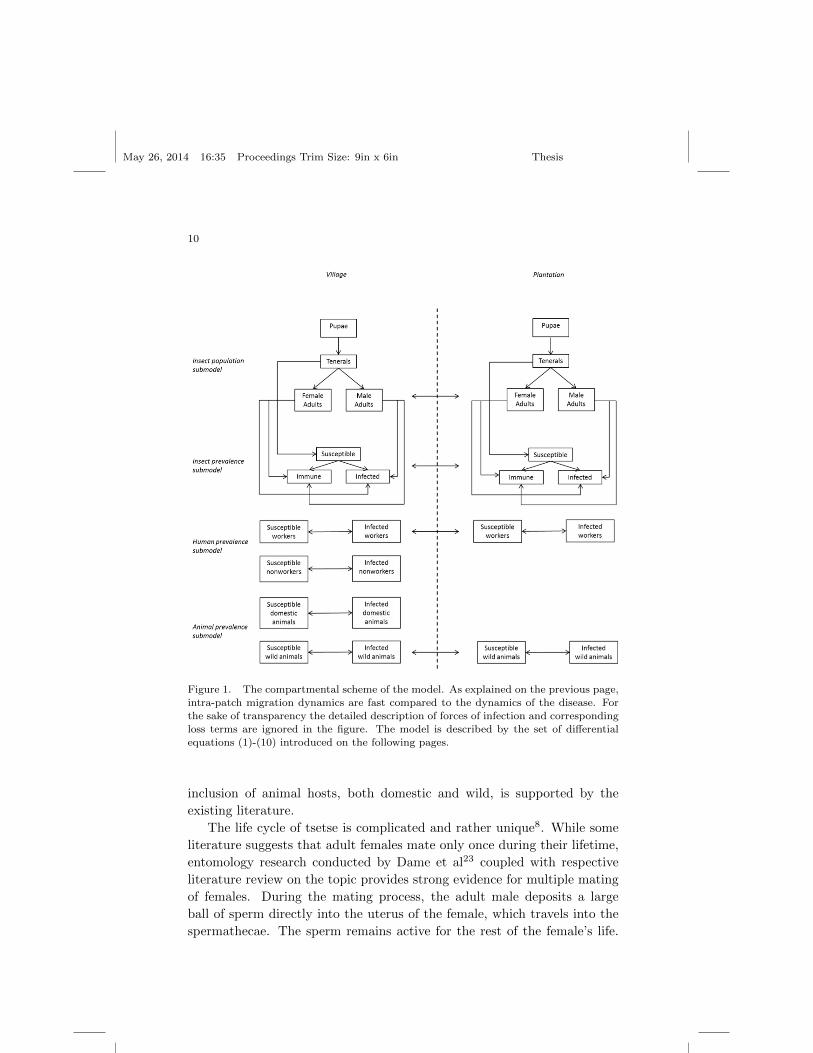
Figure 1. The compartmental scheme of the model. As explained on the previous page,
intra-patch migration dynamics are fast compared to the dynamics of the disease. Forthe sake of transparency the detailed description of forces of infection and correspondingloss terms are ignored in the figure. The model is described by the set of differential
equations (1)-(10) introduced on the following pages.
inclusion of animal hosts, both domestic and wild, is supported by the
existing literature.
The life cycle of tsetse is complicated and rather unique8. While some
literature suggests that adult females mate only once during their lifetime,
entomology research conducted by Dame et al23 coupled with respective
literature review on the topic provides strong evidence for multiple mating
of females. During the mating process, the adult male deposits a large
ball of sperm directly into the uterus of the female, which travels into the
spermathecae. The sperm remains active for the rest of the female’s life.
May 26, 2014 16:35 Proceedings Trim Size: 9in x 6in Thesis
11
Nevertheless, due to multiple mating of both males and females, part of the
deposited sperm gets replaced by the sperm of the next male. While this
nuance is irrelevant for a full population of fertile males, it becomes highly
significant if sterile males are introduced into the ecosystem. We address
this concern later in the paper during our discussion of sterile insect control
technique. The female incubates one egg at a time. The egg passes into
the uterus, where it is immediately fertilized. The egg spends four days
developing into a larva, and about five days in a combination of three
larval stages. About nine days after the egg passes into her uterus, the
female deposits the fully-grown larva from her uterus into a patch of loose,
protected soil, where it quickly develops a hard, dark shell, and becomes a
pupa. The pupal period can last from about twenty to forty days, depending
on the species, soil, humidity, and temperature8. At the end of the period,
the shell breaks and a small fly emerges.
The time between hatching and the fly’s first meal is known as the ten-
eral stage7. The first meal is very important as this food is used to develop
the flight muscles in the thorax, which are undeveloped at emergence8.
Flies are vulnerable to infection by T. brucei in this weak state, and de-
velop immunity after their first blood meal7. After the teneral stage, the
flies enter the adult stage. After mating, adult females give birth to a single
larva approximately every nine to ten days for the remainder of their lives.
Males live about three weeks. Females usually live longer, although their
life expectancy varies greatly between different species and is very sensitive
to atmospheric temperature8.
While teneral flies are rather dormant and rest up to a few days before
their first meal8, the adult flies tend to migrate daily, traveling up to several
miles. Such migrations play a vital role in the dynamics of the fly population
and the disease.
2.1.1. Equations and Parameter Values
We assume that every adult female fly mates successfully, independent of
the male population. We base this assumption on the fact that female
and male fly populations both mate multiple times and that the sperm
deposited by a single male is capable of lasting throughout the lifetime of
the female fly.
We furthermore assume that the temperature is non-constant, which
makes our model non-autonomous. The effect of temperature on the pa-
rameters within the model, however, is assumed to be linear. We describe
May 26, 2014 16:35 Proceedings Trim Size: 9in x 6in Thesis
12
each temperature-dependent parameter with a temperature-dependent lin-
ear function in order to crudely match the parameter ranges to the existing
epidemiological data. This is a significant modification from the previ-
ous range-dependent estimation and it follows the existing literature more
closely. Furthermore, this assumption allows us to generalize the model
to any set of temperature data without the need to change the parameter
values of the model.
The majority of the population models rely on a carrying capacity as-
sumption to bound population growth. However, considering the life cycle
of the tsetse fly, it is difficult to imagine what would impose such a bound.
Fly populations are observed to vary widely with respect to a variety of
factors (such as temperature, humidity, time of the day, etc.)272829 and
there appear to be plenty of mammals to provide blood meals. Further-
more, the production of pupae is so small that no constraint seems relevant
there. Therefore we do not assume any a priori bound on fly populations.
Instead, we focus on the role of temperature as a controlling factor of vector
growth and decay.
As pointed out in the introduction, the vector migrations between the
patches are assumed to be rapid relative to intra-patch dynamics and spread
of the disease. Hence, the fly population submodel describes homogeneous
compartments that are spread between the two patches at a constant pro-
portion.
Equations (1) - (4) below fully describe the vector population submodel.
The four populations are represented algebraically as follows: P for pupae,
R for teneral, F for female, and M for male.
The rate of change of pupae is determined by the rate of total population
deposition less the rate of pupae maturation and the pupal death rate.
P ′ = FI−1 − P (Q1 +Q2T )−1 − V P (1)
The rate of change of teneral population is determined by the rate of
pupae maturation into tenerals less the rate of maturation of tenerals into
adults (feeding rate) and the death rate.
R′ = P (Q1 +Q2T )−1 −R(C1 + C2T )−1 −R(H1 +H2T )−1 (2)
The rate of change of adult female population is determined by the rate
of maturation of tenerals into female adults less the death rate.
May 26, 2014 16:35 Proceedings Trim Size: 9in x 6in Thesis
13
F ′ =1
2R(C1 + C2T )−1 − F (S1 + S2T )−1 (3)
The rate of change of adult female population is determined by the rate
of maturation of tenerals into male adults less the death rate.
M ′ =1
2R(C1 + C2T )−1 −M(N1 +N2T )−1 (4)
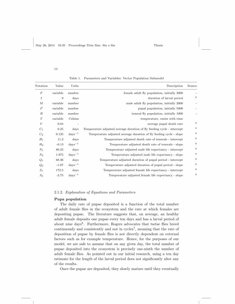
The values for all the parameters, variables, and initial conditions used
in the equations (1) - (4) are described and summarized in Table 1 below.
Table 1 provides an effective description of the parameters used in the insect
population equations, gives default values for further numerical experiments
and sources the research on which the estimates are based.
May 26, 2014 16:35 Proceedings Trim Size: 9in x 6in Thesis
14
Table 1. Parameters and Variables: Vector Population Submodel
Notation Value Units Description Source
F variable number female adult fly population, initially 3000 -
I 9 days duration of larval period 8
M variable number male adult fly population, initially 2000 -
P variable number pupal population, initially 5000 -
R variable number teneral fly population, initially 1000 -
T variable Celsius temperature, varies with time
V 0.04 - average pupal death rate 8
C1 0.25 days Temperature adjusted average duration of fly feeding cycle - intercept 8
C2 0.125 days−1 Temperature adjusted average duration of fly feeding cycle - slope 8
H1 11.2 days Temperature adjusted death rate of tenerals - intercept 8
H2 -0.13 days−1 Temperature adjusted death rate of tenerals - slope 8
N1 86.25 days Temperature adjusted male life expectancy - intercept 8
N2 1.875 days−1 Temperature adjusted male life expectancy - slope 8
Q1 68.36 days Temperature adjusted duration of pupal period - intercept 8
Q2 -1.07 days−1 Temperature adjusted duration of pupal period - slope 8
S1 172.5 days Temperature adjusted female life expectancy - intercept 8
S2 -3.75 days−1 Temperature adjusted female life expectancy - slope 8
2.1.2. Explanation of Equations and Parameters
Pupa population
The daily rate of pupae deposited is a function of the total number
of adult female flies in the ecosystem and the rate at which females are
depositing pupae. The literature suggests that, on average, an healthy
adult female deposits one pupae every ten days and has a larval period of
about nine days8. Furthermore, Rogers advocates that tsetse flies breed
continuously and consistently and not in cycles7, meaning that the rate of
deposition of pupae by female flies is not directly dependent on external
factors such as for example temperature. Hence, for the purposes of our
model, we are safe to assume that on any given day, the total number of
pupae deposited into the ecosystem is precisely one-ninth the number of
adult female flies. As pointed out in our initial research, using a ten day
estimate for the length of the larval period does not significantly alter any
of the results.
Once the pupae are deposited, they slowly mature until they eventually
May 26, 2014 16:35 Proceedings Trim Size: 9in x 6in Thesis
15
emerge into tenerals. The rate of such emergence depends on the climate
conditions, especially on atmospheric temperature. For our species, on av-
erage, the length of such period is 25-30 days87. However, entomological
research conducted by WHO suggests that the length of the so-called pupal
period is longer than average during the periods of lower temperatures and
shorter during the periods of higher temperatures8. According to the lit-
erature, the pupal period ranges between twenty-three days at the average
temperature of 33 degrees Celsius and thirty-eight days at the average tem-
perature of 19 degrees Celsius8. To model such behavior, we assumed that
the relationship between the average rate of daily emergence of pupae and
daily temperature is linear. While such assumption is indeed an estimate,
there is no entomological research in existence that would provide a bet-
ter approximation. Hence, for the sake of simplicity and in order to avoid
making unnecessary and unfounded assumptions, linearity is assumed. This
is a slight revision from the previous research done by the authors where
the temperature served as a correction factor, mainly to address our lack
of data collected and research done on the local temperature behavior at
that point. As our temperature data and model is now more sophisticated
and researched, we now feel confident enough to remove the unnecessary
additional restriction and rely completely on the temperature to serve as
an implicit boundary and accelerator to growth. Hence, using our pupal
period range as the source of data we obtain a first degree polynomial ap-
proximation for the relationship between the temperature and the pupal
period and used the estimate to approximate the emergence of flies from
pupae into tenerals. Due to lack of available data, the method yields highly
approximate results. However, the negative relationship between the du-
ration of the pupal period and the average temperature is established and
addressed within the scope of the existing research.
Because the pupae can die in many ways (parasites, predators, flooding,
and dehydration are all established causes of pupal death8) and because the
precise impact of these threats is not well known, the daily death rate of
pupae is difficult to estimate. Furthermore, some data even suggests that
pupal death rate might be correlated with temperature, beyond the impact
of the temperature extremes8. Entomological research conducted by the
WHO yields inconclusive results as at the end of four-month long rainy
season, when the pupae was collected for the count, about half of pupae
collected were found dead. At other times, however, all pupae were found
to give rise to adult flies8. Assuming a fixed rate of pupae deposition,
we estimate that about eight percent of pupae would need to die with
May 26, 2014 16:35 Proceedings Trim Size: 9in x 6in Thesis
16
each generation (about ten generations in four months) in order for the
researchers to find as many dead pupae as living ones at the end of a
four month long rainy season. Coupling this estimate with the rest of the
entomological research that found no dead pupae, we decide to fix our
estimate for pupae death at four percent. Again, while this estimate tries
to make the best out of the data available, it is still highly approximate
and there is need for further field research on the topic.
Teneral population
Tenerals are the flies that have successfully emerged from pupae and
have not yet taken their first blood meal. The teneral stage is a very
delicate stage of the flys life cycle as the flies are atypically weak before
they take their first meal, sometimes needing to rest up to a few days
before gathering the strength to fly to the nearest available host. Tenerals
emerge from pupae at the rate that was discussed in the previous paragraph
- the pupae loss term due to emergence is identical to teneral gain term.
Teneral loss term is dependent on the properties of the fly’s feeding cycle as
the teneral emerges into an adult fly immediately after its first blood meal.
The literature suggests that the frequency of biting and consequently the
rate of emergence of tenerals into adults is temperature dependent8. Low
temperatures increase the amount of time that the flies can last without a
blood meal and high temperatures tend to have the opposite effect8. While
there is no data available for our specific species, the existing research
indicates about a 20% fluctuation in the duration of the feeding cycle.
Hence, coupling this estimate with the average estimate for the length of
the feeding cycle (provided by Rogers) of four days7, we again approximate
the relationship between emergence into adults and temperature with a
first degree polynomial. Following the same procedure as before, we obtain
an estimate for the relationship between temperature and teneral death
rate, since as mentioned previously, tenerals are especially prone to external
influences and climate plays an important role in determining their survival
rate.
Female adult population
Adult fly population is a function of two terms, the emergence of tenerals
into adults and the death rate. The emergence of tenerals is, as discussed
above, dependent on temperature and varies significantly with time. For
the purposes of our model, we assume that half of the tenerals emerged
develop into female adult flies, while the other half develops into males.
Much like for tenerals, the death rate of adult females is believed to
be temperature dependent as well. In our previous research, we made an
May 26, 2014 16:35 Proceedings Trim Size: 9in x 6in Thesis
17
assumption that the relationship between temperature and female adults
death rate is quadratic in its nature. After a careful review of the literature,
we now change this assumption and instead adopt linearity. Following
our intuition from the previous paragraphs, flies indeed tend to live longer
during low temperatures and shorter during high temperatures8. There is
however, field evidence for the quadratic relationship between temperature
and fly activity as flies tend to be the most active when the temperature
is in intermediate range8. Hence, based on further research, we revise the
female adult death term and approximate it with a first degree polynomial.
Male adult population
The dynamics of the adult male population are quite analogous to the
dynamics of the female adults. The only significant difference is that the life
expectancy of the male adults is much shorter8. In our previous research,
we made an assumption that male adult death rate is fixed with time and
not temperature-dependent. In light of further research, we now revise
this assumption and assume a linear relationship between temperature and
death rate8. Hence, we change the dynamic of the system significantly and
hopefully enhance the ability of the model to mimic entomological reality.
2.2. Prevalence Submodels
In the previous section we developed and described an intricate insect pop-
ulation submodel for G. tachinoides. In this section we perform a similar
task as we introduce and develop five differential equations describing HAT
prevalence rates for one vector and four hosts (workers, non-workers, wild
animals, and domestic animals) for a medium-sized West African village
that is a few miles away from a proportionately-sized plantation. Hence,
our prevalence submodels strive to build on the previous research and find-
ings in order to construct a broadly useful model.
In order to address the importance of vector migration and to investigate
the implications that it has on the disease dynamic we decide to address
spatial heterogeneity by splitting the system into two patches; village and
plantation. The choice of patches is deliberate as the existing field research
shows that tsetse flies indeed congregate around human-populated areas
with villages and plantations mentioned as principal examples8. Further-
more, this split has been introduced and defended by Chalvet-Monfray et al.
who further emphasized the inclusion of patches due to their impact on the
disease dynamic11. Nevertheless, our model builds significantly on previous
two-patch models by adopting a more realistic assumption about migrating
May 26, 2014 16:35 Proceedings Trim Size: 9in x 6in Thesis
18
human subgroups (workers vs. nonworkers). Additionally, incorporating
research presented by Funk et. al, we also assume the existence of animal
reservoir that is, just like the human population, split into a migrating and
non-migrating subgroups (domestic animals vs. wild animals).
As mentioned previously, we assume that the intra-patch disease dy-
namics are fast in the sense that the migrating groups (vectors, workers,
and wild animals) migrate between the patches fast enough to not build up
any significant difference in their prevalence between patches. We find this
assumption reasonable, since intra-patch migrations take less than a day,
while the dynamics of the disease occur on the order of weeks and months.
We also assume that the prevalence rates for the migrating groups between
the two patches are the same (perfect mixing). Again this assumption is
reasonable as the migrating groups tend to migrate not just fast, but also
quite often (on a daily basis). These same assumptions are also adopted
by Chalvet-Monfray et al11. Furthermore, the sensitivity analysis done by
Birnbaum, Cho, Madsen & Zupan on the importance of rapid and frequent
migration showed that the change in the level of mixing does not change
the behavior of the disease significantly.
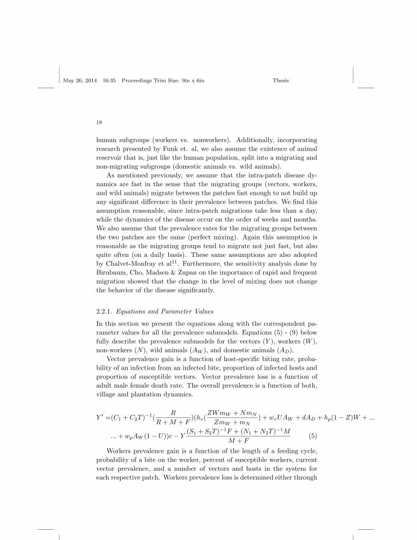
2.2.1. Equations and Parameter Values
In this section we present the equations along with the correspondent pa-
rameter values for all the prevalence submodels. Equations (5) - (9) below
fully describe the prevalence submodels for the vectors (Y ), workers (W ),
non-workers (N), wild animals (AW ), and domestic animals (AD).
Vector prevalence gain is a function of host-specific biting rate, proba-
bility of an infection from an infected bite, proportion of infected hosts and
proportion of susceptible vectors. Vector prevalence loss is a function of
adult male female death rate. The overall prevalence is a function of both,
village and plantation dynamics.
Y ′ =(C1 + C2T )−1(R
R+M + F)(hv(
ZWmW +NmN
ZmW +mN) + wvUAW + dAD + hp(1− Z)W + ...
...+ wpAW (1− U))c− Y (S1 + S2T )−1F + (N1 +N2T )−1M
M + F(5)
Workers prevalence gain is a function of the length of a feeding cycle,
probability of a bite on the worker, percent of susceptible workers, current
vector prevalence, and a number of vectors and hosts in the system for
each respective patch. Workers prevalence loss is determined either through
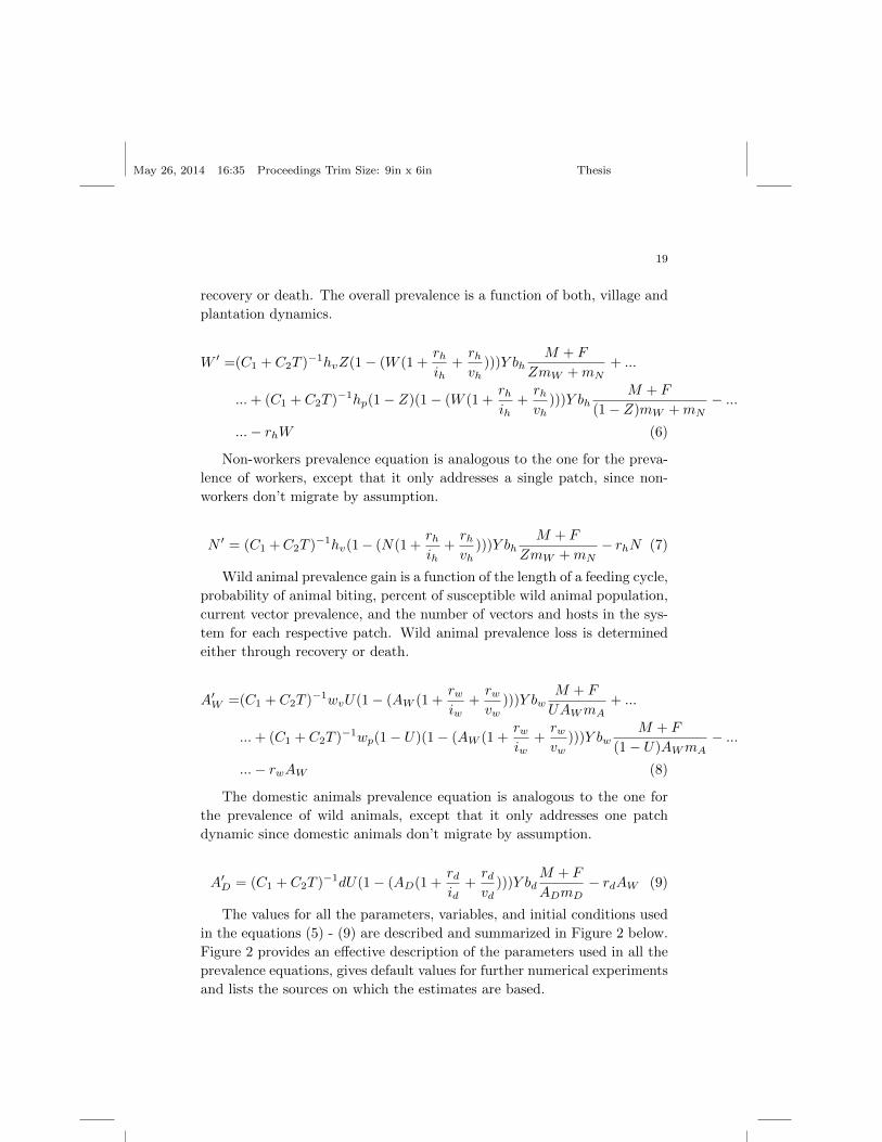
May 26, 2014 16:35 Proceedings Trim Size: 9in x 6in Thesis
19
recovery or death. The overall prevalence is a function of both, village and
plantation dynamics.
W ′ =(C1 + C2T )−1hvZ(1− (W (1 +rhih
+rhvh
)))Y bhM + F
ZmW +mN+ ...
...+ (C1 + C2T )−1hp(1− Z)(1− (W (1 +rhih
+rhvh
)))Y bhM + F
(1− Z)mW +mN− ...
...− rhW (6)
Non-workers prevalence equation is analogous to the one for the preva-
lence of workers, except that it only addresses a single patch, since non-
workers don’t migrate by assumption.
N ′ = (C1 +C2T )−1hv(1− (N(1 +rhih
+rhvh
)))Y bhM + F
ZmW +mN− rhN (7)
Wild animal prevalence gain is a function of the length of a feeding cycle,
probability of animal biting, percent of susceptible wild animal population,
current vector prevalence, and the number of vectors and hosts in the sys-
tem for each respective patch. Wild animal prevalence loss is determined
either through recovery or death.
A′W =(C1 + C2T )−1wvU(1− (AW (1 +rwiw
+rwvw
)))Y bwM + F
UAWmA+ ...
...+ (C1 + C2T )−1wp(1− U)(1− (AW (1 +rwiw
+rwvw
)))Y bwM + F
(1− U)AWmA− ...
...− rwAW (8)
The domestic animals prevalence equation is analogous to the one for
the prevalence of wild animals, except that it only addresses one patch
dynamic since domestic animals don’t migrate by assumption.
A′D = (C1 + C2T )−1dU(1− (AD(1 +rdid
+rdvd
)))Y bdM + F
ADmD− rdAW (9)
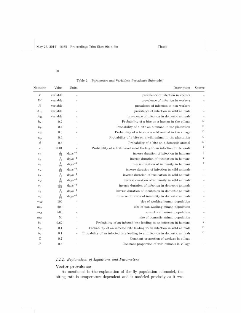
The values for all the parameters, variables, and initial conditions used
in the equations (5) - (9) are described and summarized in Figure 2 below.
Figure 2 provides an effective description of the parameters used in all the
prevalence equations, gives default values for further numerical experiments
and lists the sources on which the estimates are based.
May 26, 2014 16:35 Proceedings Trim Size: 9in x 6in Thesis
20
Table 2. Parameters and Variables: Prevalence Submodel
Notation Value Units Description Source
Y variable - prevalence of infection in vectors -
W variable - prevalence of infection in workers -
N variable - prevalence of infection in non-workers -
AW variable - prevalence of infection in wild animals -
AD variable - prevalence of infection in domestic animals -
hv 0.2 - Probability of a bite on a human in the village 10
hp 0.4 - Probability of a bite on a human in the plantation 10
wv 0.3 - Probability of a bite on a wild animal in the village 10
wp 0.6 - Probability of a bite on a wild animal in the plantation 10
d 0.5 - Probability of a bite on a domestic animal 10
c 0.01 - Probability of a first blood meal leading to an infection for tenerals 7
rh170
days−1 inverse duration of infection in humans 7
ih112
days−1 inverse duration of incubation in humans 7
vh150
days−1 inverse duration of immunity in humans 7
rw160
days−1 inverse duration of infection in wild animals -
iw112
days−1 inverse duration of incubation in wild animals -
vw150
days−1 inverse duration of immunity in wild animals -
rd1
100days−1 inverse duration of infection in domestic animals -
id112
days−1 inverse duration of incubation in domestic animals -
vd150
days−1 inverse duration of immunity in domestic animals -
mW 100 - size of working human population -
mN 200 - size of non-working human population -
mA 500 - size of wild animal population -
mD 50 - size of domestic animal population -
bh 0.62 - Probability of an infected bite leading to an infection in humans 7
bw 0.1 - Probability of an infected bite leading to an infection in wild animals 10
bd 0.1 - Probability of an infected bite leading to an infection in domestic animals 10
Z 0.7 - Constant proportion of workers in village -
U 0.5 - Constant proportion of wild animals in village -
2.2.2. Explanation of Equations and Parameters
Vector prevalence
As mentioned in the explanation of the fly population submodel, the
biting rate is temperature-dependent and is modeled precisely as it was
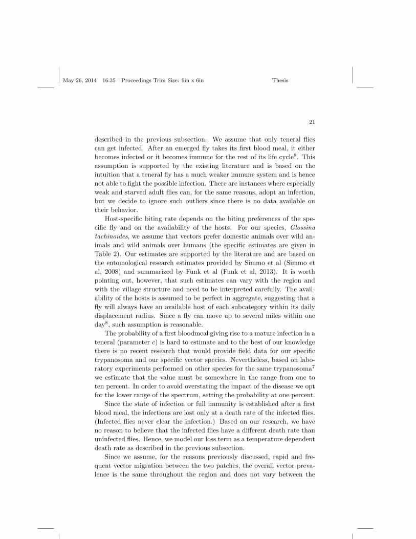
May 26, 2014 16:35 Proceedings Trim Size: 9in x 6in Thesis
21
described in the previous subsection. We assume that only teneral flies
can get infected. After an emerged fly takes its first blood meal, it either
becomes infected or it becomes immune for the rest of its life cycle8. This
assumption is supported by the existing literature and is based on the
intuition that a teneral fly has a much weaker immune system and is hence
not able to fight the possible infection. There are instances where especially
weak and starved adult flies can, for the same reasons, adopt an infection,
but we decide to ignore such outliers since there is no data available on
their behavior.
Host-specific biting rate depends on the biting preferences of the spe-
cific fly and on the availability of the hosts. For our species, Glossina
tachinoides, we assume that vectors prefer domestic animals over wild an-
imals and wild animals over humans (the specific estimates are given in
Table 2). Our estimates are supported by the literature and are based on
the entomological research estimates provided by Simmo et al (Simmo et
al, 2008) and summarized by Funk et al (Funk et al, 2013). It is worth
pointing out, however, that such estimates can vary with the region and
with the village structure and need to be interpreted carefully. The avail-
ability of the hosts is assumed to be perfect in aggregate, suggesting that a
fly will always have an available host of each subcategory within its daily
displacement radius. Since a fly can move up to several miles within one
day8, such assumption is reasonable.
The probability of a first bloodmeal giving rise to a mature infection in a
teneral (parameter c) is hard to estimate and to the best of our knowledge
there is no recent research that would provide field data for our specific
trypanosoma and our specific vector species. Nevertheless, based on labo-
ratory experiments performed on other species for the same trypanosoma7
we estimate that the value must be somewhere in the range from one to
ten percent. In order to avoid overstating the impact of the disease we opt
for the lower range of the spectrum, setting the probability at one percent.
Since the state of infection or full immunity is established after a first
blood meal, the infections are lost only at a death rate of the infected flies.
(Infected flies never clear the infection.) Based on our research, we have
no reason to believe that the infected flies have a different death rate than
uninfected flies. Hence, we model our loss term as a temperature dependent
death rate as described in the previous subsection.
Since we assume, for the reasons previously discussed, rapid and fre-
quent vector migration between the two patches, the overall vector preva-
lence is the same throughout the region and does not vary between the
May 26, 2014 16:35 Proceedings Trim Size: 9in x 6in Thesis
22
patches.
Human prevalence
We divide our human population into workers who migrate between the
two patches and non-workers, who remain in the village. The length of
the feeding cycle is a temperature-dependent parameter that determines
the frequency of biting and has been discussed in detail previously. In our
model we multiply its inverse by a probability of a bite on a worker (or
non-worker) in order to obtain the daily number of bites for a single fly
and for a single host. As suggested in Table 2, these biting probabilities
depend on whether a person is located on the plantation or in the village.
Since plantations have open space with fewer animals than a village, the
workers that migrate to work experience biting much more frequently than
non-workers. Hence, it should be no surprise to expect different prevalence
rates between the workers and non-workers.
In order to arrive to the number of infected bites taken by a fly on
a specific host, we need to multiply the number of overall bites with the
overall prevalence rate for vectors and with the overall ratio of the host
population that is susceptible to an infection. This will in turn allow us to
calculate the number of infections raised in a specific host by a single fly as
we multiply the expression with the probability of a random infected bite
leading to an infection. Lastly, in order to adjust for the total number of
vectors and hosts in the system and to arrive to the overall daily prevalence
gain we need to multiply the final calculation by the ratio of vectors to hosts.
As indicated before, the workers and non-workers will leave the infected
pool and enter the susceptible population by either recovering from the
infection or, implicitly, since the human population is assumed to remain
constant, by dying.
Animal prevalence
The submodel for animal prevalence is structurally quite similar to the
submodel for human prevalence just described. Animal population is di-
vided into two subgroups, wild animals and domestic animals, where the
wild animals migrate rapidly and frequently between the two patches and
the domestic animals remain fixed in the village. Much like the human
prevalence, animal prevalence is also a function of the length of a feeding
cycle, probability of an animal being bit, percent of susceptible animal pop-
ulation, current vector prevalence, and the number of vectors and hosts in
the system for each respective patch.
Similarly to human prevalence submodel, we first multiply the inverse
of the length of a feeding cycle by a probability of a bite on an animal in
May 26, 2014 16:35 Proceedings Trim Size: 9in x 6in Thesis
23
order to obtain the daily number of bites for a single fly on a single host.
The biting probabilities for animal subpopulations are crude estimates and
depend on the region and on the type of the animal, as pigs, for example,
tend to have a higher biting probability than sheep10. In our model we
assume an average village with equally many wild and domestic animals
distribution.
Following the same process described for human prevalence submodel,
we arrive at the overall daily prevalence gains for the domestic and wild
animals. Due to migration, the wild animal subpopulation dynamic is a
slightly more complex than the domestic animal model, but follows the
same underlying intuition.
Both domestic and wild animals will leave the infected pool and en-
ter the susceptible population by either recovering from the infection or
implicitly, by dying, since the population is assumed to remain constant.
2.3. Temporal Stochastic Temperature Model
The duration of almost every stage in the tsetse lifecycle is temperature-
dependent8. Temperature is considered to be the most important character-
istic of the thermodynamic state of the atmosphere, as it influences other
atmospheric factors such as humidity, air pressure, and precipitation12.
Hence, temperature helps us to understand and explain the impact of the
atmosphere and its elements on the behavior of the tsetse fly. In fact,
our previous research has shown that temperature plays a crucial role not
just in its impact on the behavior of the tsetse fly, but also in its effect
on the behavior of the disease25. Understanding the importance of the
temperature, we decided to put extensive focus on the construction of a
temperature model that will allow us to rigorously investigate the impact
of the temperature variation on the behavior of the system. Relying on the
spatial-temporal stochastic model with seasonal variance for daily average
temperature data presented by Benth et al12, we construct a comprehensive
model that allows us to control for trend, seasonality, mean reversion, and
seasonally dependent variance of the residuals. We present and introduce
the model in this subsection.
We fit the suggested model to the average daily temperature data col-
lected in Tillabri, Niger for the period from 1968-1980. This site was chosen
deliberately, as it is in the center of the region in which our species of fly,
G. tachinoides, is located. The model and the attendant MATLAB code,
however, were designed generically to fit a model for any input data period
May 26, 2014 16:35 Proceedings Trim Size: 9in x 6in Thesis
24
and for any region.
The original model presented by Benth et al.12 extends the model to
the spatial domain, which would allow us to control for region dependency.
However, this property is dropped for the purposes of our analysis, as the
behavior of the tsetse species is region-dependent8 and our model is not
sufficiently sophisticated to model this behavior. For regions that vary
significantly in their natural characteristics (such as for example size, types
of flora and fauna, and the type of soil), a vector population model needs
to be amended accordingly. However, if the regions explored have similar
characteristics, the temperature model can be easily extended to account
for spatial dependency of temperature.
2.3.1. Benth’s Model, Amended
We now present an amended version of the model presented by Benth et
al12. For the original version and its applications, please refer to the original
paper. In order to construct a spatiotemporal temperature model, we must
first define the spatial-temporal Gaussian random field. For the sake of
clarity, we keep the notation consistent with the model proposed by Benth
et al.
{Z(s, t) : s ∈ D ⊂ R2, t ∈ {0,∞)
}(10)
where s and t describe spatial and temporal coordinates, respectively12.
Since our analysis we focus on one specific location (which is assumed to
be small enough that temperature is uniform), our spatial domain only has
one dimension and our model can be simply written as
Z(t) = µ(t) + ε(t) (11)
where Z(t) is a time series temperature data (for the specific spatial
location), µ(t) denotes the mean process, and ε(t) denotes the residual
process. The mean process can be further described as
µ(t) = S(t) + α(Z(t− 1)− S(t− 1)), (12)
where
S(t) = l(t) + s(t). (13)
May 26, 2014 16:35 Proceedings Trim Size: 9in x 6in Thesis
25
Here l(t) describes a linear trend and s(t) describes the seasonality in
daily average temperatures. The regression equations are as follows:
l(t) = a0 + a1t (14)
s(t) = b1 + b2 cos(2π(t− b3)
365). (15)
Similarly, the residual process can be given as
ε(t) = σ(t)ε(t) (16)
Where σ(t) describes a seasonally dependent standard deviation func-
tion and ε(t) is defined as a zero-mean temporally independent Gaussian
random process with standard deviation equal to 0.1.
σ2(t) = c1 +
4∑k=1
[c2k cos(
2kπt
365) + c2k+1 sin(
(2k + 1)πt
365)
](17)
2.3.2. Fitting the Model
In order to fit the model to the described daily average temperature data,
we follow a step-by-step process, analogous in structure to the process de-
scribed by Benth et al, in order to methodically estimate, account for, and
isolate each trend component contribution from the data. While this section
describes the process we followed for sake of transparency, a MATLAB pro-
gram was developed for easy reproduction of results for any daily average
temperature data. The code is attached in an appendix.
First, we estimate the linear trend and subtract the linearity from the
model. The linear trend in daily average temperature is estimated by run-
ning a simple linear regression and observing for statistically significant non-
zero results. The obtained slope is approximately equal to a1 = −0.0002
and the intercept is equal to a0 = 30.3223. Our linear regression suggests
a negative trend, which indicates a decrease in the local mean temperature
over the period. The temperature data is in degrees Celsius. Our linear
trend can be described as:
l(t) = 30.3223− 0.0002t (18)
May 26, 2014 16:35 Proceedings Trim Size: 9in x 6in Thesis
26
Second, after subtracting for linearity, we focus on the analysis of the
seasonal effects of the residuals. The residuals exhibit a clear seasonal
pattern and we now estimate this trend by fitting the residual data using
the nlinfit method in MatLab. We can then describe the seasonality trend
as:
s(t) = −0.0212− 2.9770 cos(2π(t+ 41.3777)
365)(19) (19)
Third, after subtracting for linearity and seasonality, we analyze the
linear association between lagged observations and estimate the impact
of mean-reversion on the obtained residuals. Using MATLAB, we apply
an autoregressive model of order 1 (mean-reverting model) to obtain the
coefficient value of α = 0.7979. The AR(1) model developed relied on Burgs
lattice-based method for computing the least-squares AR model.
Fourth, after subtracting for linearity, seasonality, and the impact of
mean reversion, we focus on the analysis of the residuals, ε(t). In order
to account for seasonally-dependent variance, we first average the values of
the squared residuals of the particular day for all of the years. Next we
model the obtained values through truncated Fourier function fitting. The
results for the parameters described in equation (17) are presented in Table
3.
2.3.3. Fitted Model Equations and Parameters
In this section we summarize the results of the model fitting process intro-
duced and described in the previous subsections. Our final model has been
fitted to the average daily temperature data collected in Tillabri, Niger for
the period from 1968-1980 and is fully described by the following equation:
Z(t) = a0 +a1t+b1 +b2cos(2π(t− b3)
365)+α(Z(t−1)−S(t−1))+ε(t) (20)
where σ(t) is defined as
σ2(t) = c1 +
4∑k=1
[c2k cos(
2kπt
365) + c2k+1 sin(
(2k + 1)πt
365)
](21)
and ε(t) is a zero-mean temporally independent Gaussian random pro-
cess with standard deviation of 0.1.
May 26, 2014 16:35 Proceedings Trim Size: 9in x 6in Thesis
27
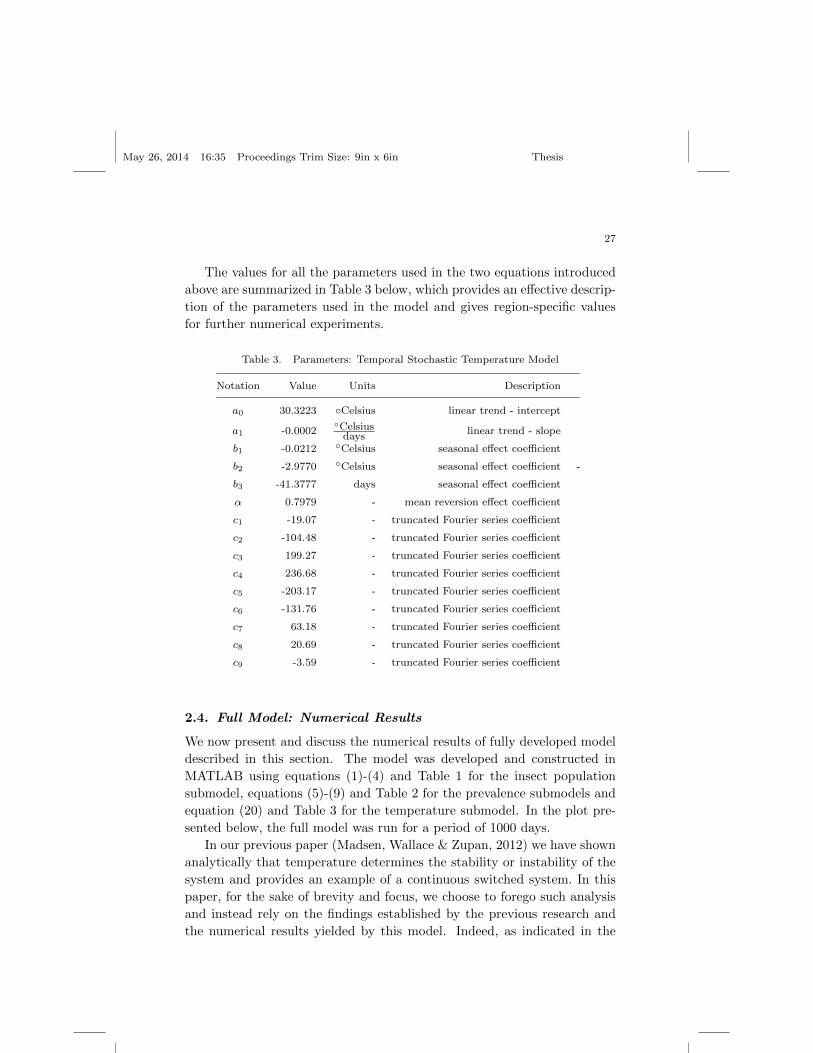
The values for all the parameters used in the two equations introduced
above are summarized in Table 3 below, which provides an effective descrip-
tion of the parameters used in the model and gives region-specific values
for further numerical experiments.
Table 3. Parameters: Temporal Stochastic Temperature Model
Notation Value Units Description
a0 30.3223 ◦Celsius linear trend - intercept
a1 -0.0002◦Celsius
dayslinear trend - slope
b1 -0.0212 ◦Celsius seasonal effect coefficient
b2 -2.9770 ◦Celsius seasonal effect coefficient -
b3 -41.3777 days seasonal effect coefficient
α 0.7979 - mean reversion effect coefficient
c1 -19.07 - truncated Fourier series coefficient
c2 -104.48 - truncated Fourier series coefficient
c3 199.27 - truncated Fourier series coefficient
c4 236.68 - truncated Fourier series coefficient
c5 -203.17 - truncated Fourier series coefficient
c6 -131.76 - truncated Fourier series coefficient
c7 63.18 - truncated Fourier series coefficient
c8 20.69 - truncated Fourier series coefficient
c9 -3.59 - truncated Fourier series coefficient
2.4. Full Model: Numerical Results
We now present and discuss the numerical results of fully developed model
described in this section. The model was developed and constructed in
MATLAB using equations (1)-(4) and Table 1 for the insect population
submodel, equations (5)-(9) and Table 2 for the prevalence submodels and
equation (20) and Table 3 for the temperature submodel. In the plot pre-
sented below, the full model was run for a period of 1000 days.
In our previous paper (Madsen, Wallace & Zupan, 2012) we have shown
analytically that temperature determines the stability or instability of the
system and provides an example of a continuous switched system. In this
paper, for the sake of brevity and focus, we choose to forego such analysis
and instead rely on the findings established by the previous research and
the numerical results yielded by this model. Indeed, as indicated in the
May 26, 2014 16:35 Proceedings Trim Size: 9in x 6in Thesis
28
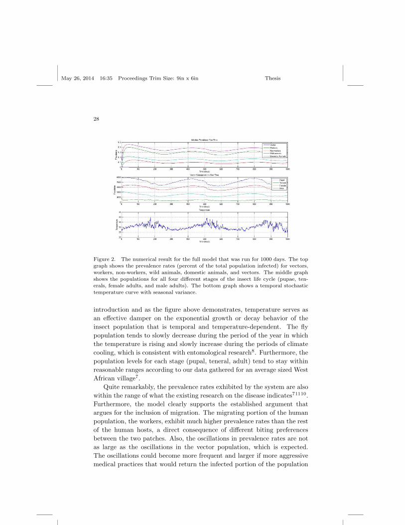
Figure 2. The numerical result for the full model that was run for 1000 days. The top
graph shows the prevalence rates (percent of the total population infected) for vectors,workers, non-workers, wild animals, domestic animals, and vectors. The middle graph
shows the populations for all four different stages of the insect life cycle (pupae, ten-
erals, female adults, and male adults). The bottom graph shows a temporal stochastictemperature curve with seasonal variance.
introduction and as the figure above demonstrates, temperature serves as
an effective damper on the exponential growth or decay behavior of the
insect population that is temporal and temperature-dependent. The fly
population tends to slowly decrease during the period of the year in which
the temperature is rising and slowly increase during the periods of climate
cooling, which is consistent with entomological research8. Furthermore, the
population levels for each stage (pupal, teneral, adult) tend to stay within
reasonable ranges according to our data gathered for an average sized West
African village7.
Quite remarkably, the prevalence rates exhibited by the system are also
within the range of what the existing research on the disease indicates71110.
Furthermore, the model clearly supports the established argument that
argues for the inclusion of migration. The migrating portion of the human
population, the workers, exhibit much higher prevalence rates than the rest
of the human hosts, a direct consequence of different biting preferences
between the two patches. Also, the oscillations in prevalence rates are not
as large as the oscillations in the vector population, which is expected.
The oscillations could become more frequent and larger if more aggressive
medical practices that would return the infected portion of the population
May 26, 2014 16:35 Proceedings Trim Size: 9in x 6in Thesis
29
back to the susceptible pool were assumed.
Unfortunately, field data on the behavior of insect population and preva-
lence rates is very scarce. Consequently it is hard to validate our model
beyond the scope of reasonable range estimates provided by the literature.
Screening is difficult, especially in vectors and wild animals. Furthermore,
due to their constant vertical and horizontal migration, the insect popu-
lation is very hard to determine with the use of conventional means such
as trapping. However, as previously mentioned, the authors feel very con-
fident about the results yielded by the model as the prevalence rates are
consistent with the estimates suggested by the literature. The domestic
animals have the highest prevalence rate, closely followed by the workers.
Both prevalence rates are on the higher end of the spectrum, but still com-
pletely plausible11. The same is true for the other two hosts, wild animals
and non-workers who are also exhibiting the behavior supported by the
established research7. In addition, vector prevalence rates, while hard to
determine in reality, fluctuate around the established values as well7.
It is also worth noting the relationships and lags between the graphs pre-
sented in Figure 2. For instance, we notice a negative relationship between
temperature and vector populations, which results in a small lag between
the temperature curve’s lowest point and the peak vector population, which
is a consequence of the tsetse reproduction cycle. There also exists a lag
between the vector population peak and the peaks in the prevalence rates,
a consequence of the dynamics of the disease. The summation of these two
lags in turn describes the impact of temperature on the the prevalence rate.
3. Analysis of Control Strategies
In this section we will further extend the model developed in the previous
section and apply it to a variety of pressing questions that have arisen in
topic literature. While we certainly will not answer all these questions, we
will provide the reader with a numerical tool to further explore them. In or-
der to motivate further research and contribute to the existing one, we will,
however, address the most interesting and important queries within each
topic. The topics included in our analysis include temperature, invasion
and barriers, trapping, live baiting, sterile insect technique, and screening.
There are a few general assumptions that we will make throughout our
analysis of the control strategies. We will assume that the controlled region
(village and plantation) is being regulated for the possible vector invasion
through either natural (ocean, dessert) or artificial (trapping, deforestation)
May 26, 2014 16:35 Proceedings Trim Size: 9in x 6in Thesis
30
barriers. This assumption will allow us to focus solely on the effect of
the specific control strategy and hold the impact of the external factors
such as invasion at a negligible level. Although grand, such assumption
is not unrealistic. In fact, effective barrier set-up reduces the probability
of invasion down to 0.00120 and effectively completely reduces the risk of
re-invasion. In addition, we will analyze the impact of control strategies
on the disease behavior in instances when invasion is not being regulated
effectively at the end of the section.
When assessing the introductory effectiveness of each control strategy,
we will assume realistic default values for the parameters that are based on
our research on the topic. Nevertheless, our model does allow user a great
deal of flexibility and the majority of the parameters can be easily adjusted
for further research on the topic.
Due to great variance in prices with respect to an organization, scale,
time of the year, quality of products, etc., we do not impose any cost
function constraints on the overall system but rather explore the overall
effectiveness of the control strategies with respect to optimization and time
efficiency. We are aware that the cost often pre-determines the extent of
a control operation and the model can be easily adjusted to account for
the cost of the operation. Furthermore, a publicly expressed priority of
several African governments, which are amongst the largest funders of the
control projects, is to eliminate the tsetse and Trypanosomiasis problem in
the shortest time possible20. Hence, for the sake of general applicability,
we decide to avoid the incorporation of potentially misleading cost-related
assumptions and instead focus on speed and effectiveness.
3.1. Temperature
Before we begin our analysis of control strategies, we choose to explore fur-
ther the role of temperature on the disease system. The role and impact of
temperature has been discussed and investigated extensively in the previ-
ous section of the paper. Hence, we utilize this portion of the paper merely
to address a possible application of the model, namely the impact of global
warming on the development of the disease. Because HAT is a disease that
is very temperature-sensitive, the global climate change will change the be-
havior of the disease significantly, pushing it to either grow or decay at a
much faster rate. In order to investigate the impact of such climate change
on the overall behavior of the system we utilize our temporal stochastic
temperature model introduced on the previous pages. This model allows
May 26, 2014 16:35 Proceedings Trim Size: 9in x 6in Thesis
31
the user to isolate and model the impact of linearity, seasonality, or variance
change on the system. For the purposes of our analysis, we merely focus on
the linearity portion of the model since the recent research published sug-
gests that the mean maximum temperatures display little or no warming30.
Hence, we assume three different scenarios: no macro change, constant ad-
ditional increase of 0.015 Celsius per year and constant additional decrease
of 0.015 Celsius per year. This change is consistent with the recent trend,
according to NASA, as the temperature has been rising at a rate of roughly
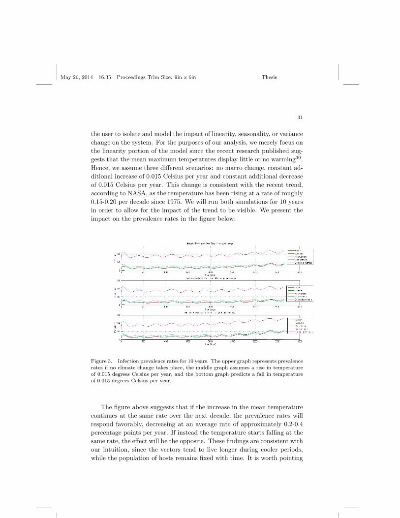
0.15-0.20 per decade since 1975. We will run both simulations for 10 years
in order to allow for the impact of the trend to be visible. We present the
impact on the prevalence rates in the figure below.
Figure 3. Infection prevalence rates for 10 years. The upper graph represents prevalencerates if no climate change takes place, the middle graph assumes a rise in temperature
of 0.015 degrees Celsius per year, and the bottom graph predicts a fall in temperatureof 0.015 degrees Celsius per year.
The figure above suggests that if the increase in the mean temperature
continues at the same rate over the next decade, the prevalence rates will
respond favorably, decreasing at an average rate of approximately 0.2-0.4
percentage points per year. If instead the temperature starts falling at the
same rate, the effect will be the opposite. These findings are consistent with
our intuition, since the vectors tend to live longer during cooler periods,
while the population of hosts remains fixed with time. It is worth pointing
May 26, 2014 16:35 Proceedings Trim Size: 9in x 6in Thesis
32
out that the effect of approximately 0.2-0.4 percentage points per year
might not seem as a big change relative to the overall prevalence rates, the
compounding effect over a longer period (few decades) can lead to much
more severe implications as demonstrated on a 10-year chart.
Other potential climate changes include increased daily or seasonal
volatility and the convergence of daily maxima and minima towards the
mean30. While we do not explore such possibilities, our model can easily
be adapted to simulate such possibilities.
3.2. Trapping
Trapping is the first of the four control strategies we will analyze in this
section of the paper. Trapping is an example of a vector control strategy,
where the disease is controlled through the eradication of the tsetse flies.
We have reason to believe that vector control strategies are in fact highly
effective and the existing field studies and theoretical research suggest that
there exists a linear relationship between tsetse density and the likelihood
of Trypanosomiasis transmission20.
Trapping is one of the cheapest, oldest, and most well spread control
tactics used to both, manage and eradicate the populations of tsetse. The
idea of traps is based on the fact that tsetse flies only feed on vertebrate
hosts and have hence evolved to detect the possible victims through the
use of their senses. An effective trap, hence, mimics the key features of
host animals through odor, color, and shape in order to attract the hungry
flies20. Basic traps function purely through the use of visual stimuli, but
their effectiveness can be significantly boosted through the use of odors.
The traps kill the flies by either entrapping them or through the use of
insecticides.
There are several downsides to trapping, when compared to some other
control strategies. Depending on their quality, the tsetse traps are quite
prone to physical degradation and can sometimes even be subject to ani-
mal and wind damage and even theft. Although minimal, deployment and
maintenance of traps does require skilled and available personnel 20. The
effectiveness of traps is a function of the density of traps, density of the
vector, likelihood of encounter and the longitude of the traps.
3.2.1. Trapping Assumptions, Parameters, and Equations
We assume that the optimal density of trapping for our species is four
traps per square kilometer. We base our assumption of optimal density
May 26, 2014 16:35 Proceedings Trim Size: 9in x 6in Thesis
33
on the research provided by Hargrove16 and Dransfield31 who discovered
that an increased density of traps within the range of attraction has stark
diminishing marginal returns. An optimal trap density is such that the
maximum distance between any two traps is smaller than the expected
daily displacement of the fly. With evenly distributed traps at the density
of four traps per square kilometer and with the range of attractiveness of one
tenth of a kilometer20, the maximum distance between two traps is 0.253km.
Since our species, Glossina tachinoides, is expected to travel distances much
longer than that, the assumption of four traps per square kilometer is more
than sufficient. Hence, within each expected daily displacement our species
of fly is almost guaranteed to encounter a trap.
Our general model allows us to uniquely incorporate each control strat-
egy at a fundamental level. Given that the traps are mimicking a vertebrate
host, we adopt an assumption that traps are part of the host dynamic with
a certain proportion of vectors biting on the traps every day. Of course
this proportion is smaller than the proportion of bites taken on actual ver-
tebrate hosts. In our model our default assumption is that the flies will
bite on traps 10% of the time. This assumption can be easily modified if
better and more expensive traps are introduced. We furthermore assume
that every fly that feeds on the trap is guaranteed to die, an assumption
that is consistent with the literature20.
We furthermore assume that the biting preferences are homogeneously
distributed throughout the region, with the flies equally likely to bite on the
plantation and on the village. This assumption seems reasonable since the
two main congregation points for flies are indeed villages and plantations8
We also allow for the various proportions of area to be covered in traps
under the same assumptions as described above. Hence, our model allows
for the possibility that only a certain part of the region (e.g. 40% of the total
area) contains traps. Our default assumption is that the trapping occurs
throughout the entire region, although some recent literature suggests that
such a deployment is unlikely to be maintained efficiently20.
As mentioned before, the traps require constant maintenance since they
are prone to physical damage. Consequently, our model allows controlling
for the number of days that the traps are being maintained for with the
default assumption being consistent with the literature and set at 365 days.
As observed in the previous section vector population fluctuates signif-
icantly with temperature; consequently the timing of trap deployment is
important. In light of this fact, our model allows controlling for the start
date in order to optimize the effect of trapping.
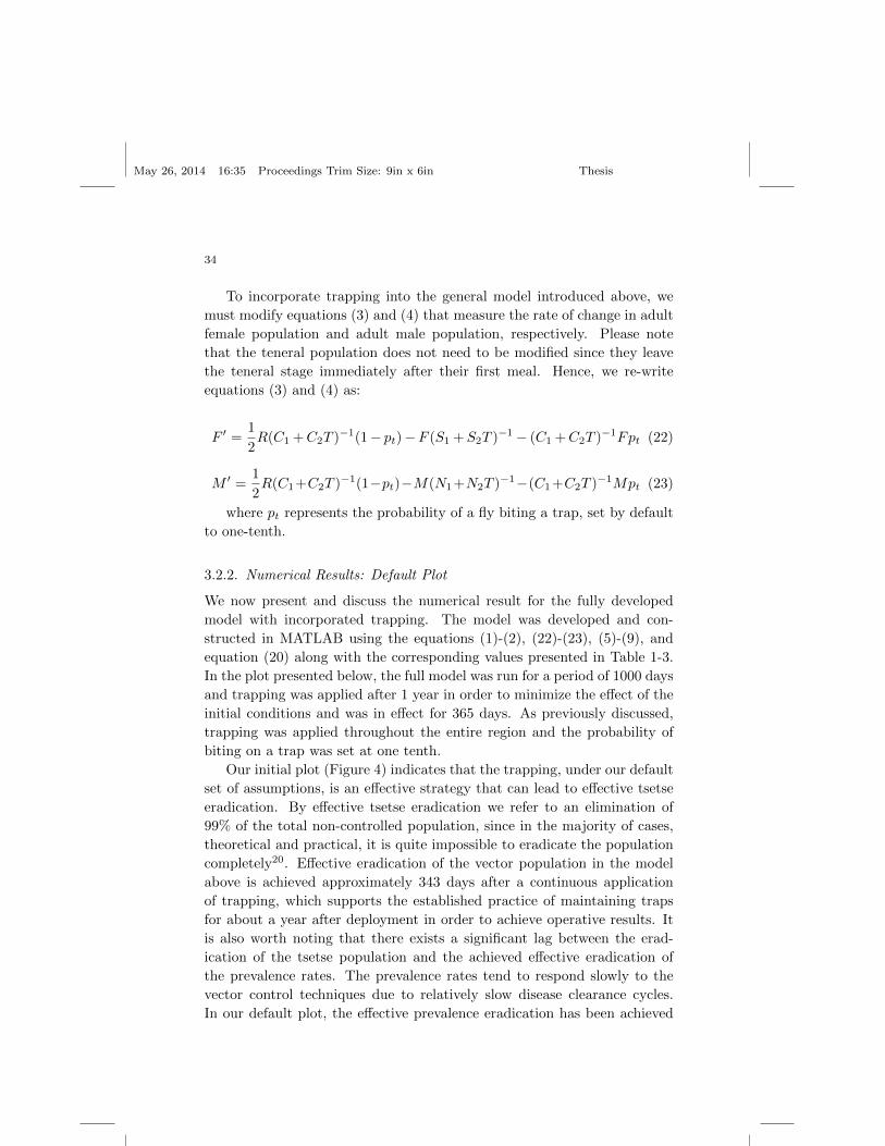
May 26, 2014 16:35 Proceedings Trim Size: 9in x 6in Thesis
34
To incorporate trapping into the general model introduced above, we
must modify equations (3) and (4) that measure the rate of change in adult
female population and adult male population, respectively. Please note
that the teneral population does not need to be modified since they leave
the teneral stage immediately after their first meal. Hence, we re-write
equations (3) and (4) as:
F ′ =1
2R(C1 +C2T )−1(1− pt)−F (S1 +S2T )−1− (C1 +C2T )−1Fpt (22)
M ′ =1
2R(C1+C2T )−1(1−pt)−M(N1+N2T )−1−(C1+C2T )−1Mpt (23)
where pt represents the probability of a fly biting a trap, set by default
to one-tenth.
3.2.2. Numerical Results: Default Plot
We now present and discuss the numerical result for the fully developed
model with incorporated trapping. The model was developed and con-
structed in MATLAB using the equations (1)-(2), (22)-(23), (5)-(9), and
equation (20) along with the corresponding values presented in Table 1-3.
In the plot presented below, the full model was run for a period of 1000 days
and trapping was applied after 1 year in order to minimize the effect of the
initial conditions and was in effect for 365 days. As previously discussed,
trapping was applied throughout the entire region and the probability of
biting on a trap was set at one tenth.
Our initial plot (Figure 4) indicates that the trapping, under our default
set of assumptions, is an effective strategy that can lead to effective tsetse
eradication. By effective tsetse eradication we refer to an elimination of
99% of the total non-controlled population, since in the majority of cases,
theoretical and practical, it is quite impossible to eradicate the population
completely20. Effective eradication of the vector population in the model
above is achieved approximately 343 days after a continuous application
of trapping, which supports the established practice of maintaining traps
for about a year after deployment in order to achieve operative results. It
is also worth noting that there exists a significant lag between the erad-
ication of the tsetse population and the achieved effective eradication of
the prevalence rates. The prevalence rates tend to respond slowly to the
vector control techniques due to relatively slow disease clearance cycles.
In our default plot, the effective prevalence eradication has been achieved
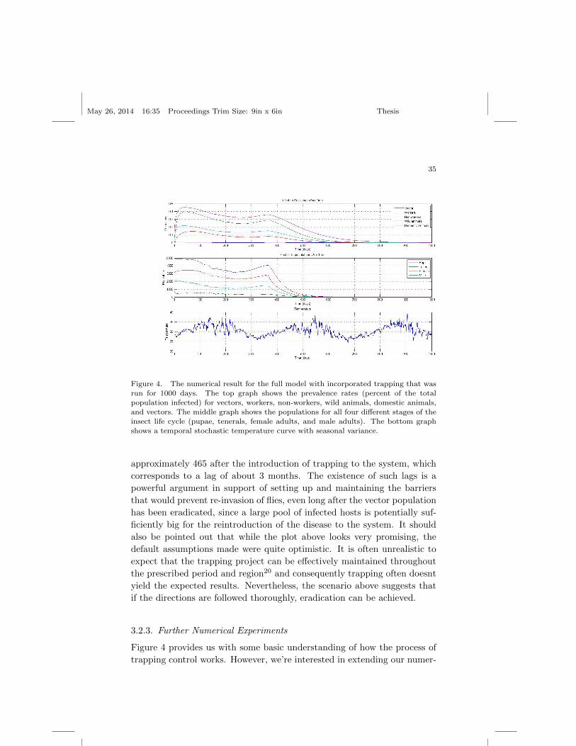
May 26, 2014 16:35 Proceedings Trim Size: 9in x 6in Thesis
35
Figure 4. The numerical result for the full model with incorporated trapping that wasrun for 1000 days. The top graph shows the prevalence rates (percent of the total
population infected) for vectors, workers, non-workers, wild animals, domestic animals,and vectors. The middle graph shows the populations for all four different stages of the
insect life cycle (pupae, tenerals, female adults, and male adults). The bottom graph
shows a temporal stochastic temperature curve with seasonal variance.
approximately 465 after the introduction of trapping to the system, which
corresponds to a lag of about 3 months. The existence of such lags is a
powerful argument in support of setting up and maintaining the barriers
that would prevent re-invasion of flies, even long after the vector population
has been eradicated, since a large pool of infected hosts is potentially suf-
ficiently big for the reintroduction of the disease to the system. It should
also be pointed out that while the plot above looks very promising, the
default assumptions made were quite optimistic. It is often unrealistic to
expect that the trapping project can be effectively maintained throughout
the prescribed period and region20 and consequently trapping often doesnt
yield the expected results. Nevertheless, the scenario above suggests that
if the directions are followed thoroughly, eradication can be achieved.
3.2.3. Further Numerical Experiments
Figure 4 provides us with some basic understanding of how the process of
trapping control works. However, we’re interested in extending our numer-
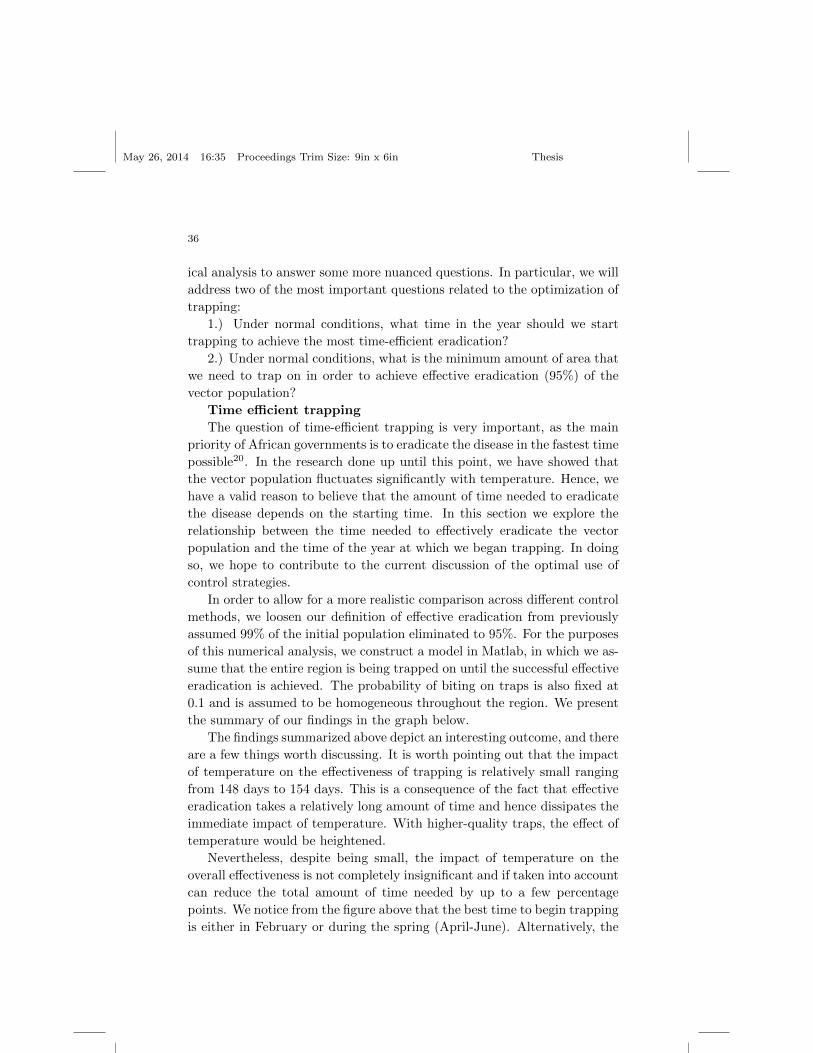
May 26, 2014 16:35 Proceedings Trim Size: 9in x 6in Thesis
36
ical analysis to answer some more nuanced questions. In particular, we will
address two of the most important questions related to the optimization of
trapping:
1.) Under normal conditions, what time in the year should we start
trapping to achieve the most time-efficient eradication?
2.) Under normal conditions, what is the minimum amount of area that
we need to trap on in order to achieve effective eradication (95%) of the
vector population?
Time efficient trapping
The question of time-efficient trapping is very important, as the main
priority of African governments is to eradicate the disease in the fastest time
possible20. In the research done up until this point, we have showed that
the vector population fluctuates significantly with temperature. Hence, we
have a valid reason to believe that the amount of time needed to eradicate
the disease depends on the starting time. In this section we explore the
relationship between the time needed to effectively eradicate the vector
population and the time of the year at which we began trapping. In doing
so, we hope to contribute to the current discussion of the optimal use of
control strategies.
In order to allow for a more realistic comparison across different control
methods, we loosen our definition of effective eradication from previously
assumed 99% of the initial population eliminated to 95%. For the purposes
of this numerical analysis, we construct a model in Matlab, in which we as-
sume that the entire region is being trapped on until the successful effective
eradication is achieved. The probability of biting on traps is also fixed at
0.1 and is assumed to be homogeneous throughout the region. We present
the summary of our findings in the graph below.
The findings summarized above depict an interesting outcome, and there
are a few things worth discussing. It is worth pointing out that the impact
of temperature on the effectiveness of trapping is relatively small ranging
from 148 days to 154 days. This is a consequence of the fact that effective
eradication takes a relatively long amount of time and hence dissipates the
immediate impact of temperature. With higher-quality traps, the effect of
temperature would be heightened.
Nevertheless, despite being small, the impact of temperature on the
overall effectiveness is not completely insignificant and if taken into account
can reduce the total amount of time needed by up to a few percentage
points. We notice from the figure above that the best time to begin trapping
is either in February or during the spring (April-June). Alternatively, the
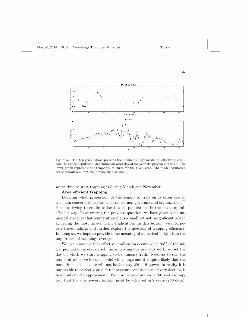
May 26, 2014 16:35 Proceedings Trim Size: 9in x 6in Thesis
37
Figure 5. The top graph above presents the number of days needed to effectively eradi-
cate the tsetse population, depending on what day of the year the process is started. Thelower graph represents the temperature curve for the given year. The model assumes a
set of default assumptions previously discussed.
worst time to start trapping is during March and November.
Area efficient trapping
Deciding what proportion of the region to trap on is often one of
the main concerns of capital-constrained non-governmental organizations20
that are trying to eradicate local tsetse populations in the most capital-
efficient way. In answering the previous question, we have given some nu-
merical evidence that temperature plays a small yet not insignificant role in
achieving the most time-efficient eradication. In this section, we incorpo-
rate these findings and further explore the question of trapping efficiency.
In doing so, we hope to provide some meaningful numerical insight into the
importance of trapping coverage.
We again assume that effective eradication occurs when 95% of the ini-
tial population is eradicated. Incorporating our previous work, we set the
day on which we start trapping to be January 29th. Needless to say, the
temperature curve for our model will change and it is quite likely that the
most time-efficient date will not be January 29th. However, in reality it is
impossible to perfectly predict temperature conditions and every decision is
hence inherently approximate. We also incorporate an additional assump-
tion that the effective eradication must be achieved in 2 years (730 days).
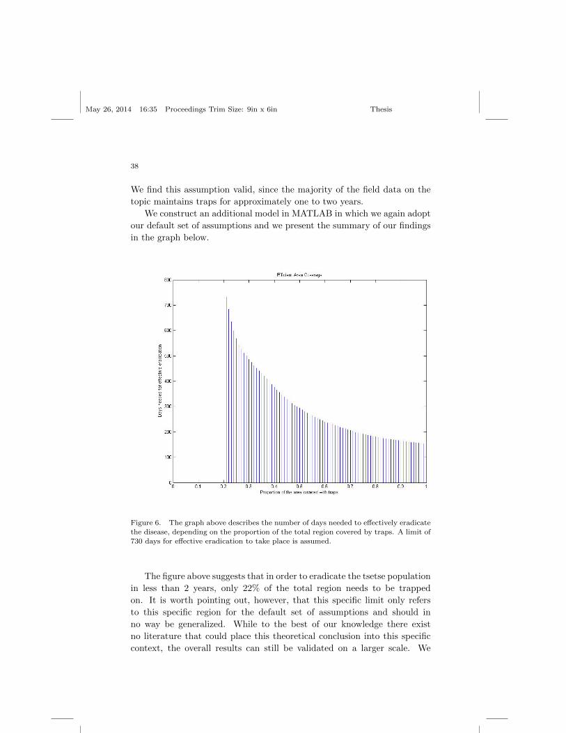
May 26, 2014 16:35 Proceedings Trim Size: 9in x 6in Thesis
38
We find this assumption valid, since the majority of the field data on the
topic maintains traps for approximately one to two years.
We construct an additional model in MATLAB in which we again adopt
our default set of assumptions and we present the summary of our findings
in the graph below.
Figure 6. The graph above describes the number of days needed to effectively eradicate
the disease, depending on the proportion of the total region covered by traps. A limit of730 days for effective eradication to take place is assumed.
The figure above suggests that in order to eradicate the tsetse population
in less than 2 years, only 22% of the total region needs to be trapped
on. It is worth pointing out, however, that this specific limit only refers
to this specific region for the default set of assumptions and should in
no way be generalized. While to the best of our knowledge there exist
no literature that could place this theoretical conclusion into this specific
context, the overall results can still be validated on a larger scale. We
May 26, 2014 16:35 Proceedings Trim Size: 9in x 6in Thesis
39
notice that if approximately 45% of the region or more is covered in traps,
the population will effectively be eradicated in less than a year. Hence, the
model supports the general conclusions of the existing field research and
control implementation attempts that managed to reach success during
comparable time intervals on a comparable scale.
Furthermore, the authors believe that a general relationship between the
eradication time efficiency and the area coverage is significant and mean-
ingful. We notice from the shape of the graph that there exist significant
diminishing marginal returns to the increase in area coverage. This obser-
vation mitigates the concerns that the inaccessible parts of the regions are
not being trapped on. Nevertheless, we must bear in mind that our model
assumes homogeneous dispersion of the vector, which might not necessar-
ily be true in reality and the impact of area coverage can hence be either
reduced or amplified, depending on the situation.
3.3. Live-Bait Technique
The live bait technique, including the use of insecticide-treated cattle (ITC),
is the second of the four control strategies analyzed. ITC is another example
of a vector control strategy and is structurally very similar to trapping,
except for the fact that the traps are replaced by live cattle.
The use of insecticides applied to livestock has been developed almost
simultaneously with the development of trapping mechanisms and it has
seen a tremendous technological improvement over the past 20 years32.It is
widely believed that in areas where there are large numbers of cattle, this
is the cheapest and most effective method of vector control17.
As with trapping, the effectiveness of live bait technique is determined
by the quality of spray, pour-on or dip used. While the majority of the
commonly-used insecticides are very efficient at killing a fly upon encounter,
the products vary widely with respect to the ranges of attraction. Further-
more, an extensive amount of research has been done on the use of footbath
treatments vs. full spraying13 and the two techniques appear to yield very
comparable results.
As with any control strategy, there are several downsides to ITC. The
control strategy is much harder to manipulate and regulate than the strat-
egy involving only stationary baits. Unlike with the case of stationary
baits, it is much harder to manipulate the density of live baits, their lo-
cation, placement, and movement17. Hence, the success of ITC is often
determined by factors that cannot be easily controlled and are beyond the
May 26, 2014 16:35 Proceedings Trim Size: 9in x 6in Thesis
40
reach of the entity regulating the operation.
The effectiveness of ITC is a function of the proportion of cattle in the
region, density of the vector, likelihood of encounter and the duration of
regime maintenance.
3.3.1. Live-Bait Assumptions, Parameters, and Equations
The live-bait technique can only be applied to cattle and there is very
little field research that promises effective results when the technique is
applied to other domestic animals. Our general model assumes constant
host populations that are based on an estimate of an average sized West
African village. Hence, in order to keep the relative size of the village
constant, we incorporate the impact of the cattle population on the overall
system, by assuming that a relative proportion of the domestic animal
reservoir consists of cattle. This assumption allows us to, instead of relying
on the absolute values, incorporate the relative cattle proportions into the
system, which in turn yield more easily generalizable results. Needless to
say, some villages will have higher proportion of cattle with respect to the
rest of the domestic animal reservoir than the others. Acknowledging that
the value chosen is quite arbitrary and subject to significant change, we
decide to assume that 20% of the domestic animal consists of cattle. Thist
assumption can, of course, be easily modified within the model.
We assume that cattle are equally likely to be bitten by tsetse flies rela-
tive to the rest of the domestic animal reservoir. While this assumption is
not true for every case and depends on the insecticide being used, it is hard
to generalize about the differences between the biting preferences on dif-
ferent domestic animal species. Although the insecticide applied can often
increase the probability of cattle being bitten, the literature also suggests
that, absent insecticide treatment, a wide array of tsetse species prefer pigs
over cattle33. Hence, we decide to keep the biting probability on the entire
domestic animal reservoir the same as in the general model, at 0.5. We fur-
thermore assume that the biting preferences are homogeneously distributed
throughout the village.
As with trapping, the use of insecticides is time-consuming and requires
continuous effort to maintain the effectiveness. Depending on the type
of insecticide and the specific technique used (pour-on, dip, spray), the
insecticide remains effective for a period of approximately three to seven
days13, after which it needs to be re-applied. We optimistically assume
that the insecticide is applied regularly in order to maintain maximum
May 26, 2014 16:35 Proceedings Trim Size: 9in x 6in Thesis
41
effectiveness of the control strategy. We furthermore assume that every
fly that feeds on the insecticide treated cattle is guaranteed to die, an
assumption that is consistent with the literature.
Since the continuous application of insecticide requires time and effort,
we decide to incorporate the option to control for the number of days that
the cattle is being treated for with the default assumption being consistent
with the literature on trapping and set at 365 days (1 year).
As in the previous sections, vector population fluctuates widely with
temperature and timing of ITC is important. In light of this fact, our
model allows controlling for the start date in order to optimize the effect
of ITC.
In order to incorporate trapping into the general model introduced
above, we must modify equations (3) and (4) that measure the rate of
change in adult female population and adult male population, respectively.
Similarly to trapping, please note that the teneral population does not need
to be modified since they leave the teneral stage immediately after taking
their blood meal. Hence, we rewrite equations (3) and (4) as:
F ′ =1
2R(C1 +C2T )−1(1− 1
2dC)−F (S1 +S2T )−1− (C1 +C2T )−1F (
1
2dC)
(24)
M ′ =1
2R(C1+C2T )−1(1− 1
2dC)−M(N1+N2T )−1−(C1+C2T )−1M(
1
2dC)
(25)
where C stands for the promotion of cattle in the domestic animal pop-
ulation and is initially assumed to be one-fifth.
3.3.2. Numerical Results: Default Plot
We now present and discuss the numerical results for the full model in-
corporating ITC. The model was developed and constructed in MATLAB
using equations (1)-(2), (24)-(25), (5)-(9), and equation (20) along with the
corresponding values presented in Table 1-3. In the plot presented below,
the full model was run for a period of 1000 days and insecticide was applied
to cattle after 1 year in order to minimize the effect of the initial conditions
and was in effect for 365 days to make results comparable to trapping. As
previously discussed, ITC was applied assuming that 20% of the animal
reservoir consists of cattle.
Figure 7 indicates that, unlike trapping, ITC, under our default set
of assumptions, does not lead to effective tsetse eradication. Please note
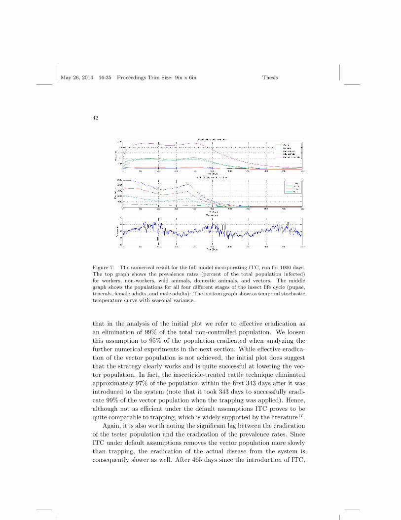
May 26, 2014 16:35 Proceedings Trim Size: 9in x 6in Thesis
42
Figure 7. The numerical result for the full model incorporating ITC, run for 1000 days.The top graph shows the prevalence rates (percent of the total population infected)
for workers, non-workers, wild animals, domestic animals, and vectors. The middlegraph shows the populations for all four different stages of the insect life cycle (pupae,
tenerals, female adults, and male adults). The bottom graph shows a temporal stochastic
temperature curve with seasonal variance.
that in the analysis of the initial plot we refer to effective eradication as
an elimination of 99% of the total non-controlled population. We loosen
this assumption to 95% of the population eradicated when analyzing the
further numerical experiments in the next section. While effective eradica-
tion of the vector population is not achieved, the initial plot does suggest
that the strategy clearly works and is quite successful at lowering the vec-
tor population. In fact, the insecticide-treated cattle technique eliminated
approximately 97% of the population within the first 343 days after it was
introduced to the system (note that it took 343 days to successfully eradi-
cate 99% of the vector population when the trapping was applied). Hence,
although not as efficient under the default assumptions ITC proves to be
quite comparable to trapping, which is widely supported by the literature17.
Again, it is also worth noting the significant lag between the eradication
of the tsetse population and the eradication of the prevalence rates. Since
ITC under default assumptions removes the vector population more slowly
than trapping, the eradication of the actual disease from the system is
consequently slower as well. After 465 days since the introduction of ITC,
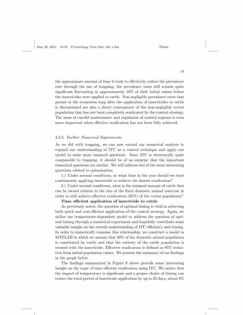
May 26, 2014 16:35 Proceedings Trim Size: 9in x 6in Thesis
43
the approximate amount of time it took to effectively reduce the prevalence
rate through the use of trapping, the prevalence rates still remain quite
significant fluctuating at approximately 10% of their initial values before
the insecticides were applied to cattle. Non-negligible prevalence rates that
persist in the ecosystem long after the application of insecticides to cattle
is discontinued are also a direct consequence of the non-negligible vector
population that has not been completely eradicated by the control strategy.
The issue of careful maintenance and regulation of control regimes is even
more important when effective eradication has not been fully achieved.
3.3.3. Further Numerical Experiments
As we did with trapping, we can now extend our numerical analysis to
expand our understanding of ITC as a control technique and apply our
model to some more nuanced questions. Since ITC is structurally quite
comparable to trapping, it should be of no surprise that the important
numerical questions are similar. We will address two of the most interesting
questions related to optimization:
1.) Under normal conditions, at what time in the year should we start
continuously applying insecticide to achieve the fastest eradication?
2.) Under normal conditions, what is the minimal amount of cattle that
can be owned relative to the size of the fixed domestic animal reservoir in
order to still achieve effective eradication (95%) of the vector population?
Time efficient application of insecticide to cattle
As previously noted, the question of optimal timing is vital in achieving
both quick and cost-efficient application of the control strategy. Again, we
utilize our temperature-dependent model to address the question of opti-
mal timing through a numerical experiment and hopefully contribute some
valuable insight on the overall understanding of ITC efficiency and timing.
In order to numerically examine this relationship, we construct a model in
MATLAB in which we assume that 20% of the domestic animal population
is constituted by cattle and that the entirety of the cattle population is
treated with the insecticide. Effective eradication is defined as 95% reduc-
tion from initial population values. We present the summary of our findings
in the graph below.
The findings summarized in Figure 8 above provide some interesting
insight on the topic of time efficient eradication using ITC. We notice that
the impact of temperature is significant and a proper choice of timing can
reduce the total period of insecticide application by up to 25 days, about 8%
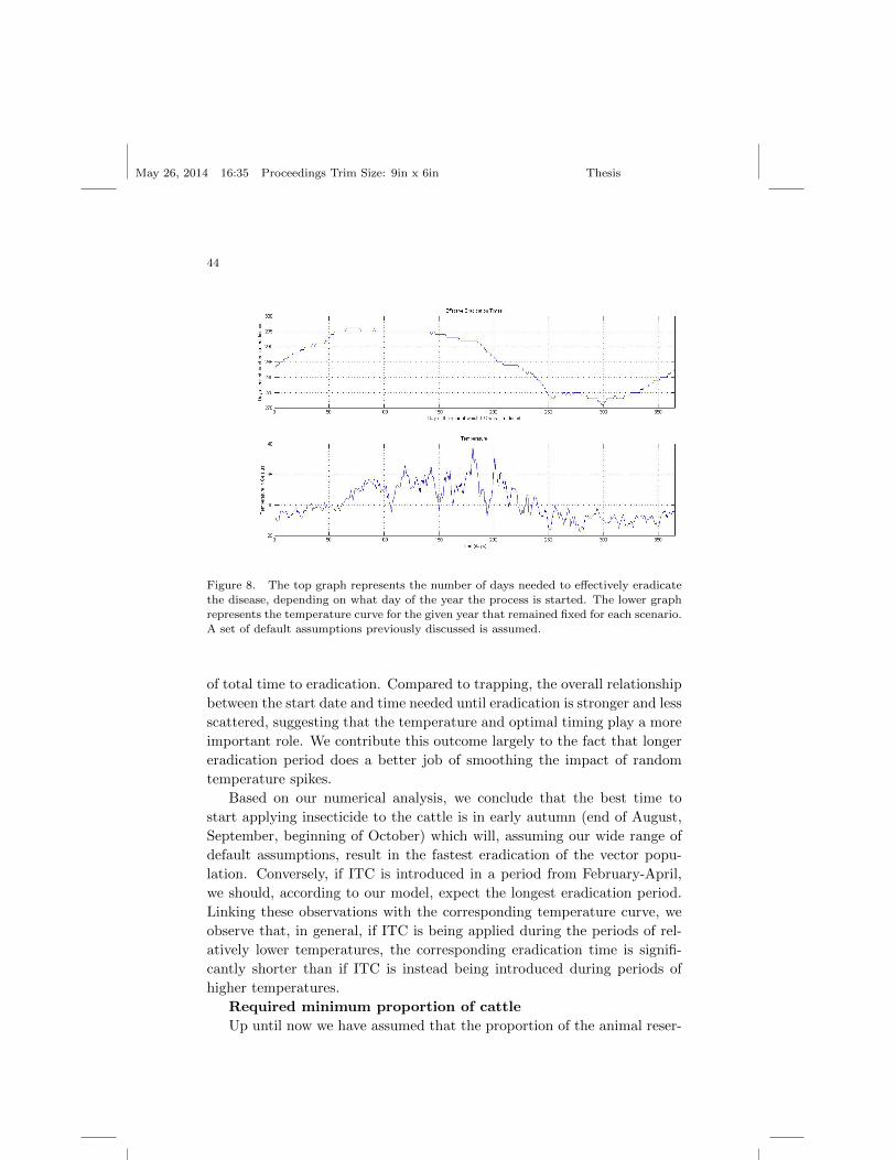
May 26, 2014 16:35 Proceedings Trim Size: 9in x 6in Thesis
44
Figure 8. The top graph represents the number of days needed to effectively eradicate
the disease, depending on what day of the year the process is started. The lower graphrepresents the temperature curve for the given year that remained fixed for each scenario.
A set of default assumptions previously discussed is assumed.
of total time to eradication. Compared to trapping, the overall relationship
between the start date and time needed until eradication is stronger and less
scattered, suggesting that the temperature and optimal timing play a more
important role. We contribute this outcome largely to the fact that longer
eradication period does a better job of smoothing the impact of random
temperature spikes.
Based on our numerical analysis, we conclude that the best time to
start applying insecticide to the cattle is in early autumn (end of August,
September, beginning of October) which will, assuming our wide range of
default assumptions, result in the fastest eradication of the vector popu-
lation. Conversely, if ITC is introduced in a period from February-April,
we should, according to our model, expect the longest eradication period.
Linking these observations with the corresponding temperature curve, we
observe that, in general, if ITC is being applied during the periods of rel-
atively lower temperatures, the corresponding eradication time is signifi-
cantly shorter than if ITC is instead being introduced during periods of
higher temperatures.
Required minimum proportion of cattle
Up until now we have assumed that the proportion of the animal reser-
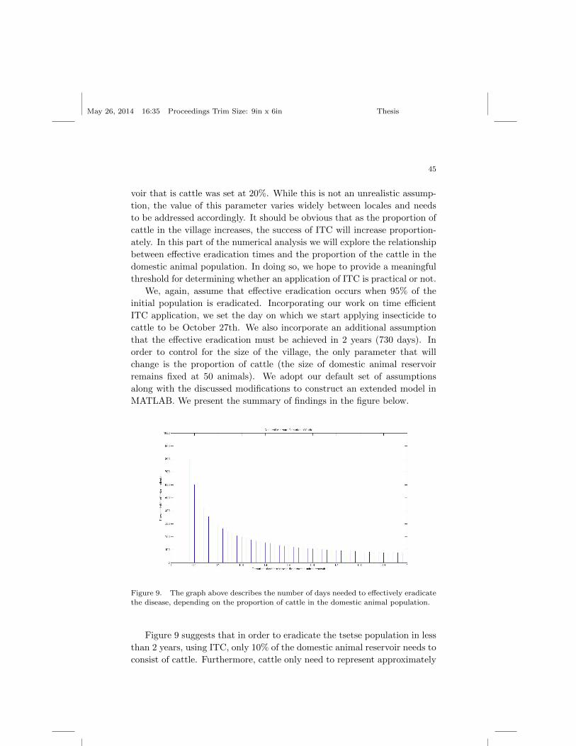
May 26, 2014 16:35 Proceedings Trim Size: 9in x 6in Thesis
45
voir that is cattle was set at 20%. While this is not an unrealistic assump-
tion, the value of this parameter varies widely between locales and needs
to be addressed accordingly. It should be obvious that as the proportion of
cattle in the village increases, the success of ITC will increase proportion-
ately. In this part of the numerical analysis we will explore the relationship
between effective eradication times and the proportion of the cattle in the
domestic animal population. In doing so, we hope to provide a meaningful
threshold for determining whether an application of ITC is practical or not.
We, again, assume that effective eradication occurs when 95% of the
initial population is eradicated. Incorporating our work on time efficient
ITC application, we set the day on which we start applying insecticide to
cattle to be October 27th. We also incorporate an additional assumption
that the effective eradication must be achieved in 2 years (730 days). In
order to control for the size of the village, the only parameter that will
change is the proportion of cattle (the size of domestic animal reservoir
remains fixed at 50 animals). We adopt our default set of assumptions
along with the discussed modifications to construct an extended model in
MATLAB. We present the summary of findings in the figure below.
Figure 9. The graph above describes the number of days needed to effectively eradicatethe disease, depending on the proportion of cattle in the domestic animal population.
Figure 9 suggests that in order to eradicate the tsetse population in less
than 2 years, using ITC, only 10% of the domestic animal reservoir needs to
consist of cattle. Furthermore, cattle only need to represent approximately
May 26, 2014 16:35 Proceedings Trim Size: 9in x 6in Thesis
46
16% of the reservoir in order to bring down the effective eradication period
under a year. It is worth pointing out, however, that this specific limit only
refers to this specific region for the default set of assumptions and should
not be freely generalized.
It is interesting to observe the shape of the relationship, which indi-
cates that ITC is almost as effective in the villages with 70% cattle as it
is in villages with cattle being the only domestic animal. This result is
viable and is a consequence of the fact that the domestic animals are only
one potential host for tsetse fly, which mitigates the impact of cattle pro-
portion increase. Furthermore, the observed relationship suggests that the
proportion of cattle does need not to be large for ITC to be effective. This
observation mitigates the concerns that only the villages with very high
proportion of cattle should be pursuing ITC.
We also notice that as the proportion of cattle increases, the period
needed for effective eradication is effectively reduced below the period
needed for eradication under trapping. This observation is consistent with
literature and field data that indicate that for certain villages with high
proportion of cattle, ITC is a faster and more effective control strategy
than trapping17.
3.4. The Sterile Insect Technique
The sterile insect technique (SIT) is the third of the four control strategies
that we will analyze and the last example of a vector control strategy con-
sidered herein. While not as old or widespread as trapping and ITC, the
concept of releasing sterile insects into wild populations has been around
since for at least seventy years34. An extensive amount of research has been
done on the topic and the process of SIT application is well understood.
The underlying principle of SIT is that fertile adult tsetse female flies
are incapable, to a certain extent, of producing larvae after they have mated
with a sexually sterile male. The process of sterilization of adult males is
usually completed through mutagenic agent treatment, such as for example
gamma radiation or chemosterilants application35. After such treatment,
the sterile males are released into the wild to freely mate with the wild
adult female flies. The success of the entire process is heavily dependent
on the assumption that the sterile males, aside from being infertile, display
the same behavior as their wild equivalents35. Although the literature re-
viewed usually adopts such an assumption as valid, there are some authors
that account for poor performance of sterile males when compared to wild
May 26, 2014 16:35 Proceedings Trim Size: 9in x 6in Thesis
47
counterparts19.
As with any control strategy, there are several shortcomings to using
SIT. When compared to trapping and ICT, SIT is usually a much more
expensive and less accessible control method, especially when the area
controlled is large17. Furthermore, effective eradication is usually easier
achieve through the use of more conventional control methods. Although
not often17, SIT can be used to achieve effective eradication of the vector,
although it is more often used to merely reduce insect populations to very
low levels35. Nevertheless, it is also worth mentioning that the use of SIT is
rather environmentally friendly and it does not assume any of the risk that
the flies treated with insecticides will develop resistance to the chemicals.
The effectiveness of SIT is a function of the number of sterile males
released compared to the overall vector population, the overall comparable
performance of sterile males relative to their wild counterparts, frequency
of mating, and replacement proportion of previously deposited sperm.
3.4.1. SIT Assumptions, Parameters, and Equations
We assume that sterile males introduced into the system exhibit poor per-
formance relative to their wild counterparts. We incorporate this assump-
tion to be consistent with the majority of the recent literature on mathe-
matical modelling19 that strives not to overstate the impact of SIT on the
vector population. Hence, consistent with literature, we assume that the
sterile males have 25% greater death rate than their wild counterparts19. If
other control strategies are introduced into the system the sterile and wild
males are equally susceptible to their impact.
The females inseminated by sterile males have a high chance of becom-
ing infertile. Nevertheless, the fertilization process is rather complicated
and further assumptions need to be addressed. A large portion of entomo-
logical research on tsetse fly behavior seems to suggest that female flies only
mate once in their lifetime. In fact, in our previous research on the topic,
relying on such literature, the authors have made a similar assumption25.
While this assumption was rather irrelevant up until now and has not im-
pacted the overall behavior results, we must now take special care to revise
it appropriately. Based on the entomological research provided by Dame
and Ford23 we are able to conclude that an assumption of multiple mat-
ing is valid. It is worth noting that had we not changed our assumption
from previous research, our results of SIT effectiveness would be decid-
edly skewed. Although the research provided by Dame was performed on
May 26, 2014 16:35 Proceedings Trim Size: 9in x 6in Thesis
48
a different species of tsetse fly than assumed in our model, we base our
parameter estimates on their results, due to the lack of better data. We do,
however, acknowledge that such parameter estimates are very approximate
and need to be subject to further revisions as more research is done on the
topic. Basing our estimates on the lab experiments presented by Dame and
Ford, we conclude that a female that has mated with a sterile male first and
fertile male second will deposit the pupa 44.7% of the time. Conversely, a
female fly that has first mated with a fertile male and with a sterile male
second deposits a pupa, on average, 85% of the time23. No change in pupa
deposition rate is assumed if the fertility of consecutive male mating part-
ners does not change and the flies are assumed to mate, on average, every
three days.
Mating probability is a direct function of the size of sterile male and
wild male populations, an assumption consistent with what is suggested in
the literature23. Hence, a simplifying assumption is made that if a female
was last inseminated by a sterile male it will assume the pupa production
capacity of a previously assumed infertile female. If conversely, a female was
last inseminated by a wild male, it will assume the fertile rate of production
of pupa. It needs to be stated that such an assumption ignores some of the
nuances related to mating process and sperm replacement rates for tsetse
flies as there exist proven diminishing returns23. However, as pointed out
previously, since such data is not available for our specific species, we avoid
making unnecessary ungrounded assumptions and instead assume linearity.
Acknowledging the complexity of the discussed technique we build our
model in such a way to allow the researchers to freely determine the number
of releases, the number of males released, the possible increase in releases,
and the starting time of SIT. We do not, however, allow for variance in
the intervals between the consecutive releases since our research indicates
suggest that this is difficult to control. Hence we assume that the males are
released weekly, basing our parameter estimate on the model introduced by
Vale and Torr19.
While we allow for a free modification of the parameters described
above, we also provide the initial parameter estimates (default values)
based on the existing research done on the topic to stimulate the discussion.
Hence, we set the number of males(mi) released each interval at three times
the population of wild males (about six thousand), a ratio that Vale and
Torr found to be an optimal estimate19. We furthermore set the rate of
increase (mr) in size of successive releases to be zero, consistent with Vale
and Torr. The number of weekly releases (RW ) is initially set at six.
May 26, 2014 16:35 Proceedings Trim Size: 9in x 6in Thesis
49
Our vector population submodel allows us to uniquely incorporate the
impact of sterile male releases into the system by more precisely modelling
their overall behavior. In order to incorporate SIT into the system, we
hence create two additional tsetse subpopulations, sterile males and infertile
females. As discussed in the previous paragraphs, aside from their infertility
(females), their sterility (males), and their weaker immune system causing
higher death rate (males), the underlying assumptions for these two stages
remain the same as for the rest of the population. We model the sterile
males (MS) with the following equation:
M ′S = mi(1 +mr)RW − 1.25(N1 +N2T )−1MS (26)
Where mi denotes the number of males released at each interval, mr
denotes the increase rate, and RW represents the number of releases. Sim-
ilarly, the infertile female (FS) rate of change is as follows:
F ′S =MS
MS +M
1
3(ffF − fiFS)− (S1 + S2T )−1FS (27)
Where ff = 0.85 and fi = 0.447 denote the ability of fertile and infertile
female flies to produce pupae, respectively. In order to account for the
impact of sterile males on wild females, we must also modify equation (3)
which models wild female population by adding a loss term to the sterile
females compartment.
F ′ =1
2R(C1 + C2T )−1 − F (S1 + S2T )−1 − MS
MS +M
1
3ffF (28)
3.4.2. Numerical Result: Default Plot
We now present and discuss the numerical results for the fully developed
model with incorporated SIT. The model was developed and constructed
in MATLAB using the equations (1)-(3), (26)-(28), (5)-(9), and equation
(20) along with the corresponding values presented in Table 1-3. In the
plot presented below, the full model was run for a period of 1000 days and
sterile males were began to be released after one year in order to minimize
the effect of the initial conditions. As previously discussed, 6000 sterile
males (3:1 ratio) were released every seven days for six consecutive weeks.
Figure 10 suggests that, under the set of our default assumptions, SIT
is unable to achieve effective eradication at both, 99% and 95% level, as
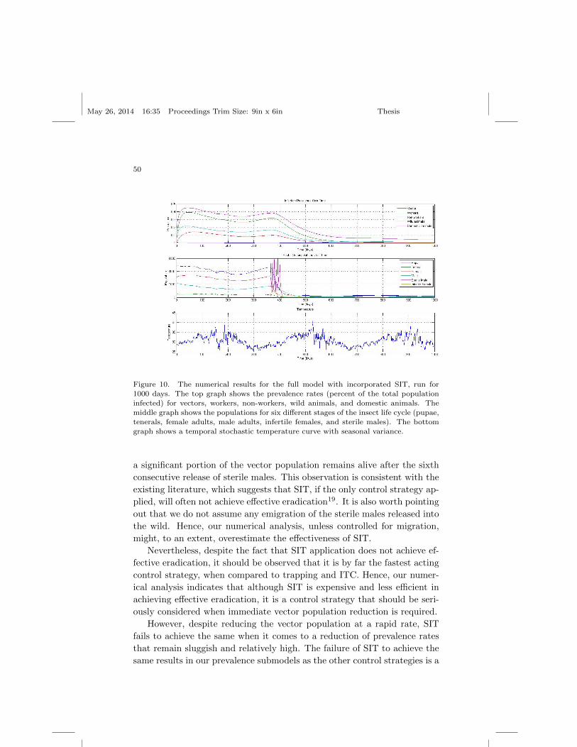
May 26, 2014 16:35 Proceedings Trim Size: 9in x 6in Thesis
50
Figure 10. The numerical results for the full model with incorporated SIT, run for1000 days. The top graph shows the prevalence rates (percent of the total population
infected) for vectors, workers, non-workers, wild animals, and domestic animals. Themiddle graph shows the populations for six different stages of the insect life cycle (pupae,
tenerals, female adults, male adults, infertile females, and sterile males). The bottom
graph shows a temporal stochastic temperature curve with seasonal variance.
a significant portion of the vector population remains alive after the sixth
consecutive release of sterile males. This observation is consistent with the
existing literature, which suggests that SIT, if the only control strategy ap-
plied, will often not achieve effective eradication19. It is also worth pointing
out that we do not assume any emigration of the sterile males released into
the wild. Hence, our numerical analysis, unless controlled for migration,
might, to an extent, overestimate the effectiveness of SIT.
Nevertheless, despite the fact that SIT application does not achieve ef-
fective eradication, it should be observed that it is by far the fastest acting
control strategy, when compared to trapping and ITC. Hence, our numer-
ical analysis indicates that although SIT is expensive and less efficient in
achieving effective eradication, it is a control strategy that should be seri-
ously considered when immediate vector population reduction is required.
However, despite reducing the vector population at a rapid rate, SIT
fails to achieve the same when it comes to a reduction of prevalence rates
that remain sluggish and relatively high. The failure of SIT to achieve the
same results in our prevalence submodels as the other control strategies is a
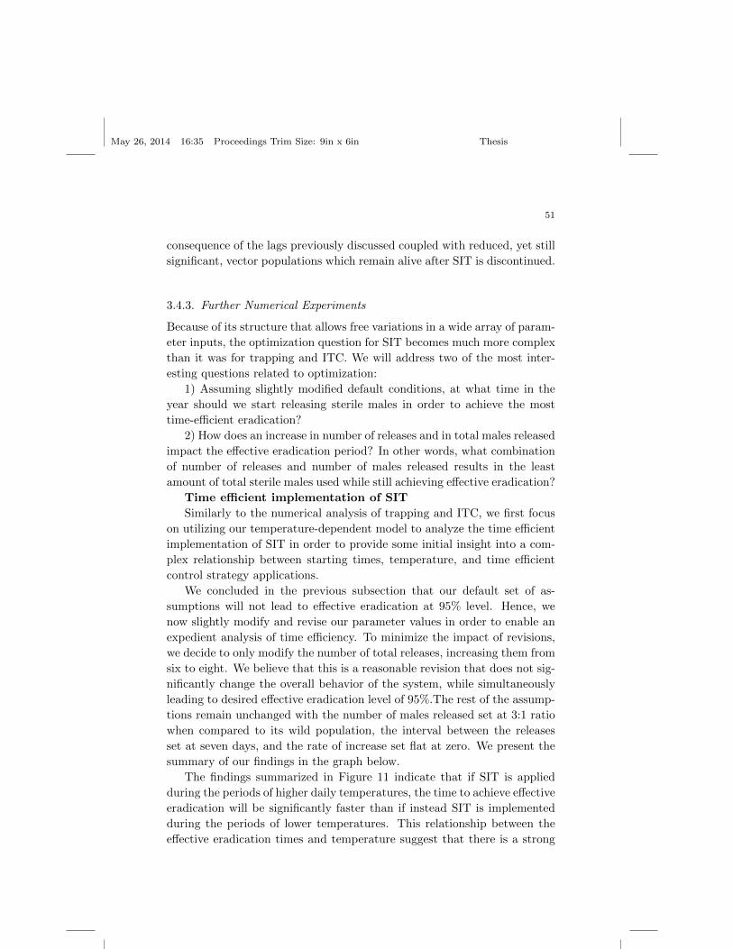
May 26, 2014 16:35 Proceedings Trim Size: 9in x 6in Thesis
51
consequence of the lags previously discussed coupled with reduced, yet still
significant, vector populations which remain alive after SIT is discontinued.
3.4.3. Further Numerical Experiments
Because of its structure that allows free variations in a wide array of param-
eter inputs, the optimization question for SIT becomes much more complex
than it was for trapping and ITC. We will address two of the most inter-
esting questions related to optimization:
1) Assuming slightly modified default conditions, at what time in the
year should we start releasing sterile males in order to achieve the most
time-efficient eradication?
2) How does an increase in number of releases and in total males released
impact the effective eradication period? In other words, what combination
of number of releases and number of males released results in the least
amount of total sterile males used while still achieving effective eradication?
Time efficient implementation of SIT
Similarly to the numerical analysis of trapping and ITC, we first focus
on utilizing our temperature-dependent model to analyze the time efficient
implementation of SIT in order to provide some initial insight into a com-
plex relationship between starting times, temperature, and time efficient
control strategy applications.
We concluded in the previous subsection that our default set of as-
sumptions will not lead to effective eradication at 95% level. Hence, we
now slightly modify and revise our parameter values in order to enable an
expedient analysis of time efficiency. To minimize the impact of revisions,
we decide to only modify the number of total releases, increasing them from
six to eight. We believe that this is a reasonable revision that does not sig-
nificantly change the overall behavior of the system, while simultaneously
leading to desired effective eradication level of 95%.The rest of the assump-
tions remain unchanged with the number of males released set at 3:1 ratio
when compared to its wild population, the interval between the releases
set at seven days, and the rate of increase set flat at zero. We present the
summary of our findings in the graph below.
The findings summarized in Figure 11 indicate that if SIT is applied
during the periods of higher daily temperatures, the time to achieve effective
eradication will be significantly faster than if instead SIT is implemented
during the periods of lower temperatures. This relationship between the
effective eradication times and temperature suggest that there is a strong
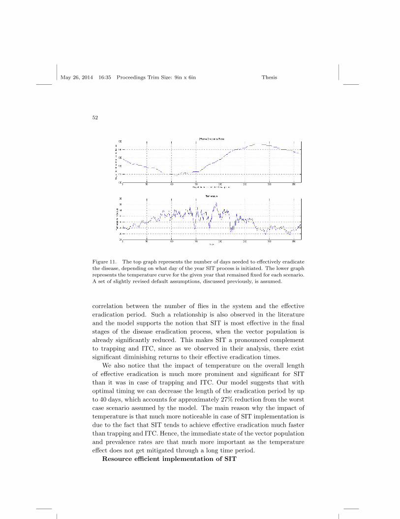
May 26, 2014 16:35 Proceedings Trim Size: 9in x 6in Thesis
52
Figure 11. The top graph represents the number of days needed to effectively eradicate
the disease, depending on what day of the year SIT process is initiated. The lower graphrepresents the temperature curve for the given year that remained fixed for each scenario.
A set of slightly revised default assumptions, discussed previously, is assumed.
correlation between the number of flies in the system and the effective
eradication period. Such a relationship is also observed in the literature
and the model supports the notion that SIT is most effective in the final
stages of the disease eradication process, when the vector population is
already significantly reduced. This makes SIT a pronounced complement
to trapping and ITC, since as we observed in their analysis, there exist
significant diminishing returns to their effective eradication times.
We also notice that the impact of temperature on the overall length
of effective eradication is much more prominent and significant for SIT
than it was in case of trapping and ITC. Our model suggests that with
optimal timing we can decrease the length of the eradication period by up
to 40 days, which accounts for approximately 27% reduction from the worst
case scenario assumed by the model. The main reason why the impact of
temperature is that much more noticeable in case of SIT implementation is
due to the fact that SIT tends to achieve effective eradication much faster
than trapping and ITC. Hence, the immediate state of the vector population
and prevalence rates are that much more important as the temperature
effect does not get mitigated through a long time period.
Resource efficient implementation of SIT
May 26, 2014 16:35 Proceedings Trim Size: 9in x 6in Thesis
53
In our analysis of SIT up until now, we have held fixed the majority of
the parameters that can be varied such as number of releases and males
released. In this part of the analysis, however, we explore the role of these
parameters with respect to time efficiency and optimal resource allocation.
In performing such numerical analysis, we strive to provide some important
insight into how should the control strategy be implemented in order to
optimize the amount of resources used and time spent.
We, again, assume that effective eradication occurs when 95% of the
initial population is eradicated. Incorporating our work on time efficient
SIT application, we set the day on which we start implementing SIT to
be April 20th. We furthermore assume, as previously discussed, that the
rate of increase remains flat and that the males are released every 7 days.
We then vary the number of releases and the number of males released
and explore the impact of these incremental changes on the corresponding
effective eradication rates. This analysis allows us to determine the most
resource-efficient and time-efficient combination of varied parameter values.
We present the summary of findings in the figure below.
Figure 12. The graph on the left represents how the effective eradication times vary
with respect to the number of releases and number of males released with each release.
The graph on the right complements it as it represents the total number of sterile malesthat needed to be used for each of such scenarios.
The two graphs in figure 12 above offer an interesting perspective. Our
May 26, 2014 16:35 Proceedings Trim Size: 9in x 6in Thesis
54
numerical analysis suggests that the number of releases plays a much more
prominent role in determining the resource efficiency than the number of
males released during each interval. As few as 10,000 sterile males total
are needed to eradicate the disease if they are released at the rate of 1,000
males per interval. Quite reasonably, however, the most resource efficient
approach is also the slowest, as it achieves effective eradication 48 days later
(approximately 52% longer) than the fastest and most resource intensive
approach.
Conversely, the graph on the left indicates that the time-efficient erad-
ication strategy is much more sensitive to the increase in the number of
sterile males released at each interval. We link this fact to the point made
in the previous subsection, where our analysis showed that the overall ratio
of sterile to wild males plays a crucial role in determining the overall erad-
ication period. Hence, our analysis further supports the argument that the
absolute and relative time efficiency of SIT increases proportionally with
the size of the regions.
3.5. Screening
Screening is the fourth and the last control strategy introduced, described,
and analyzed in this work. Unlike the first three control strategies analyzed,
screening is not an example of a vector control strategy. Screening instead
targets the human reservoir directly and is generally introduced to reduce
mortality by identifying cases early and to reduce future transmission rates
by eliminating a portion of the infectious host reservoir 18.
T.b. gambiense HAT, the chronic version of HAT, has two stages: the
first or hemolymphatic stage and the second or neurological stage of the
disease. In the first stage of the disease, patients experience nonspecific
symptoms such as fever, headaches, arthralgia, and enlarged cervical lymph
nodes. In the second stage, psychiatric, sensory, and motor functions are
interrupted, and if left untreated, the patients die due to eventual dys-
function of the immune system 15. The process of screening is non-trivial
and the disease is diagnosed in three steps: screening, diagnostic confirma-
tion, and staging (first or second stage)15. The majority of active screening
methods are based on mass case detection and must hence be affordable,
quick, sensitive, and sufficient in its capacity15.
There exist several methods for active screening. Currently, the most
well used method is Card Agglutination Test for Trypanosomiasis (CATT)
that allows hundreds of individuals to be tested daily. CATT is a simple
May 26, 2014 16:35 Proceedings Trim Size: 9in x 6in Thesis
55
agglutination for detection of antibodies in the blood, plasma, or serum
of HAT patients and its reported sensitivity varies from 87%-98%15. Nev-
ertheless, due to its sensitivity CATT remains limited as it is difficult to
apply to regions with HAT prevalence rates lower than 5%.
Once an infected individual is successfully detected through the use of
CATT or any other method, he must go through staging in order to deter-
mine a suitable treatment. If individual is in the first stage of the disease,
a 7-10 day treatment with intramuscular pentamidine is prescribed and
less than 1% chance of dying is assumed. Patients in the second stage are
instead treated with melarsorpol and 2%-10% mortality rate is assumed15
The effectiveness of screening is a function of five factors: attendance
rate, sensitivity of the screening test, sensitivity of the confirmation test,
proportion of confirmed cases that complete treatment, and cure rate18.
3.5.1. Screening Assumptions, Parameters, and Equations
In order to incorporate the impact of active screening on the overall preva-
lence in humans, we adopt a model developed by Robays et al18 in which
the otherwise complicated process of active screening is simplified and bro-
ken down into five components that in turn determine the effectiveness of
the method. As previously mentioned, the effectiveness of screening (E) is
defined as a product of attendance rate (Ar), sensitivity of the screening
test (Ss), sensitivity of the confirmation test (Sc), treatment completion
rate (Tr), and cure rate (Cr).
In their paper, Robays et al also provide a range of estimates for each
parameter. For the purposes of the thesis, we decide to assume the mean
values. In this paper we provide the readers with the chosen mean esti-
mates, but we omit the justification and the range values as they are easily
accessible in the original paper18. Hence, we obtain the following equation
for the effectiveness of active screening:
E = ArSsScTrCr (29)
The initial values are: Ar = 0.75, Ss = 0.95, Sc = 0.75, Tr = 0.9,
Cr = 0.9, and E = 0.43.
The overall success of active screening also depends on the optimal
frequency of the screening rounds, which is still poorly understood and
widely debated18. Some prominent researchers recommend three separate
screening rounds at one-year intervals, while others use 6-month intervals.
May 26, 2014 16:35 Proceedings Trim Size: 9in x 6in Thesis
56
According to Robays et. al, the most recent research assumes 6-month fre-
quency, which will be also a default parameter value for our model. We
assume that four screens are conducted, composing a two year long pro-
gram.
Since active screening is quite expensive and hard to implement within
large communities, we also incorporate an option to control for the propor-
tion of the population screened and for the population subtypes (workers
and non-workers). Since active screening programs usually strive to screen
the entire population, we assume in our default set of assumptions that the
entirety of both worker and non-worker populations are screened each time.
Although to a lesser extent our initial plot of the general model shows
fluctuations in prevalence rates due to temperature impact. Hence, in order
to address the question of optimal timing, we also allow to vary the starting
times at which the first screen is piloted.
In order to implement the discussed additional assumptions into our
model, we only need to modify the equations for the prevalence rate schange
in workers and nonworkers. Hence the modified equation for workers is
given as follows:
W ′ = (6)− sWSEW (30)
Here WS is the proportion of workers screened, E is the effectiveness of
screening, and s is the inverse frequency of the program. Similarly, if we
use NS to represent the proportion of non-workers screened, the modified
equation for non-workers is given as:
N ′ = (7)− sNSEN (31)
3.5.2. Numerical Result: Default Plot
We now present and discuss the numerical result for the fully developed
model with incorporated active human screening program. The model was
developed and constructed in MATLAB using the equations (1)-(5), (30)-
(31), (8)-(9), and equation (20) along with the corresponding values pre-
sented in Table 1-3. In the plot presented below, the full model was run for
a period of 1000 days and active screening was first piloted after one year
in order to minimize the effect of the initial conditions. As discussed pre-
viously, the program screened the entire population four times in intervals
of six months.
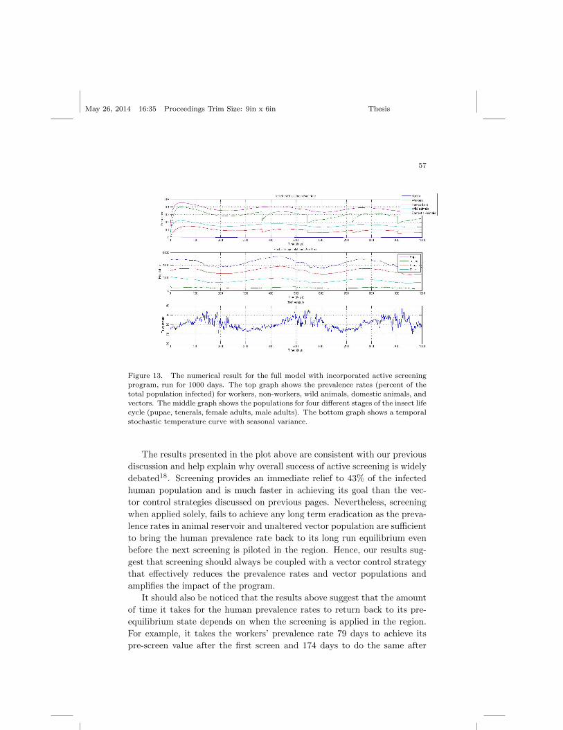
May 26, 2014 16:35 Proceedings Trim Size: 9in x 6in Thesis
57
Figure 13. The numerical result for the full model with incorporated active screeningprogram, run for 1000 days. The top graph shows the prevalence rates (percent of the
total population infected) for workers, non-workers, wild animals, domestic animals, andvectors. The middle graph shows the populations for four different stages of the insect life
cycle (pupae, tenerals, female adults, male adults). The bottom graph shows a temporal
stochastic temperature curve with seasonal variance.
The results presented in the plot above are consistent with our previous
discussion and help explain why overall success of active screening is widely
debated18. Screening provides an immediate relief to 43% of the infected
human population and is much faster in achieving its goal than the vec-
tor control strategies discussed on previous pages. Nevertheless, screening
when applied solely, fails to achieve any long term eradication as the preva-
lence rates in animal reservoir and unaltered vector population are sufficient
to bring the human prevalence rate back to its long run equilibrium even
before the next screening is piloted in the region. Hence, our results sug-
gest that screening should always be coupled with a vector control strategy
that effectively reduces the prevalence rates and vector populations and
amplifies the impact of the program.
It should also be noticed that the results above suggest that the amount
of time it takes for the human prevalence rates to return back to its pre-
equilibrium state depends on when the screening is applied in the region.
For example, it takes the workers’ prevalence rate 79 days to achieve its
pre-screen value after the first screen and 174 days to do the same after
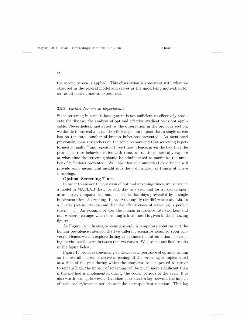
May 26, 2014 16:35 Proceedings Trim Size: 9in x 6in Thesis
58
the second screen is applied. This observation is consistent with what we
observed in the general model and serves as the underlying motivation for
our additional numerical experiment.
3.5.3. Further Numerical Experiments
Since screening in a multi-host system is not sufficient to effectively eradi-
cate the disease, the analysis of optimal effective eradication is not appli-
cable. Nevertheless, motivated by the observation in the previous section,
we decide to instead analyze the efficiency of an impact that a single screen
has on the total number of human infections prevented. As mentioned
previously, some researchers on the topic recommend that screening is per-
formed annually18 and repeated three times. Hence, given the fact that the
prevalence rate behavior varies with time, we set to numerically explore
at what time the screening should be administered to maximize the num-
ber of infections prevented. We hope that our numerical experiment will
provide some meaningful insight into the optimization of timing of active
screenings.
Optimal Screening Times
In order to answer the question of optimal screening times, we construct
a model in MATLAB that, for each day in a year and for a fixed temper-
ature curve, compares the number of infection days prevented by a single
implementation of screening. In order to amplify the differences and obtain
a clearer picture, we assume that the effectiveness of screening is perfect
(i.e.E = 1). An example of how the human prevalence rate (workers and
non-workers) changes when screening is introduced is given in the following
figure:
As Figure 14 indicates, screening is only a temporary solution and the
human prevalence rates for the two different scenarios assumed soon con-
verge. Hence, we can explore during what times the introduction of screen-
ing maximizes the area between the two curves. We present our final results
in the figure below.
Figure 15 provides convincing evidence for importance of optimal timing
on the overall success of active screening. If the screening is implemented
at a time of the year during which the temperature is expected to rise or
to remain high, the impact of screening will be much more significant than
if the method is implemented during the cooler periods of the year. It is
also worth noting, however, that there does exist a lag between the impact
of such cooler/warmer periods and the correspondent reaction. This lag
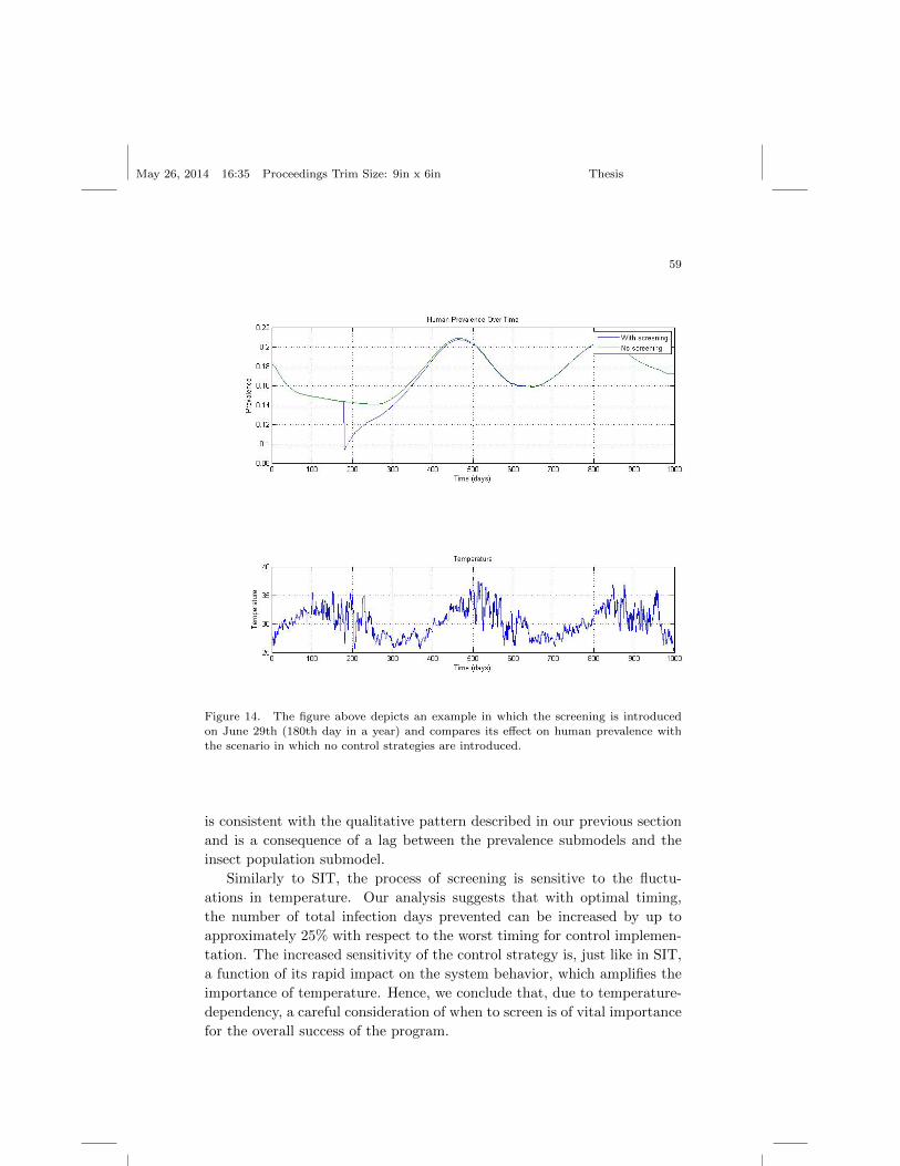
May 26, 2014 16:35 Proceedings Trim Size: 9in x 6in Thesis
59
Figure 14. The figure above depicts an example in which the screening is introduced
on June 29th (180th day in a year) and compares its effect on human prevalence withthe scenario in which no control strategies are introduced.
is consistent with the qualitative pattern described in our previous section
and is a consequence of a lag between the prevalence submodels and the
insect population submodel.
Similarly to SIT, the process of screening is sensitive to the fluctu-
ations in temperature. Our analysis suggests that with optimal timing,
the number of total infection days prevented can be increased by up to
approximately 25% with respect to the worst timing for control implemen-
tation. The increased sensitivity of the control strategy is, just like in SIT,
a function of its rapid impact on the system behavior, which amplifies the
importance of temperature. Hence, we conclude that, due to temperature-
dependency, a careful consideration of when to screen is of vital importance
for the overall success of the program.
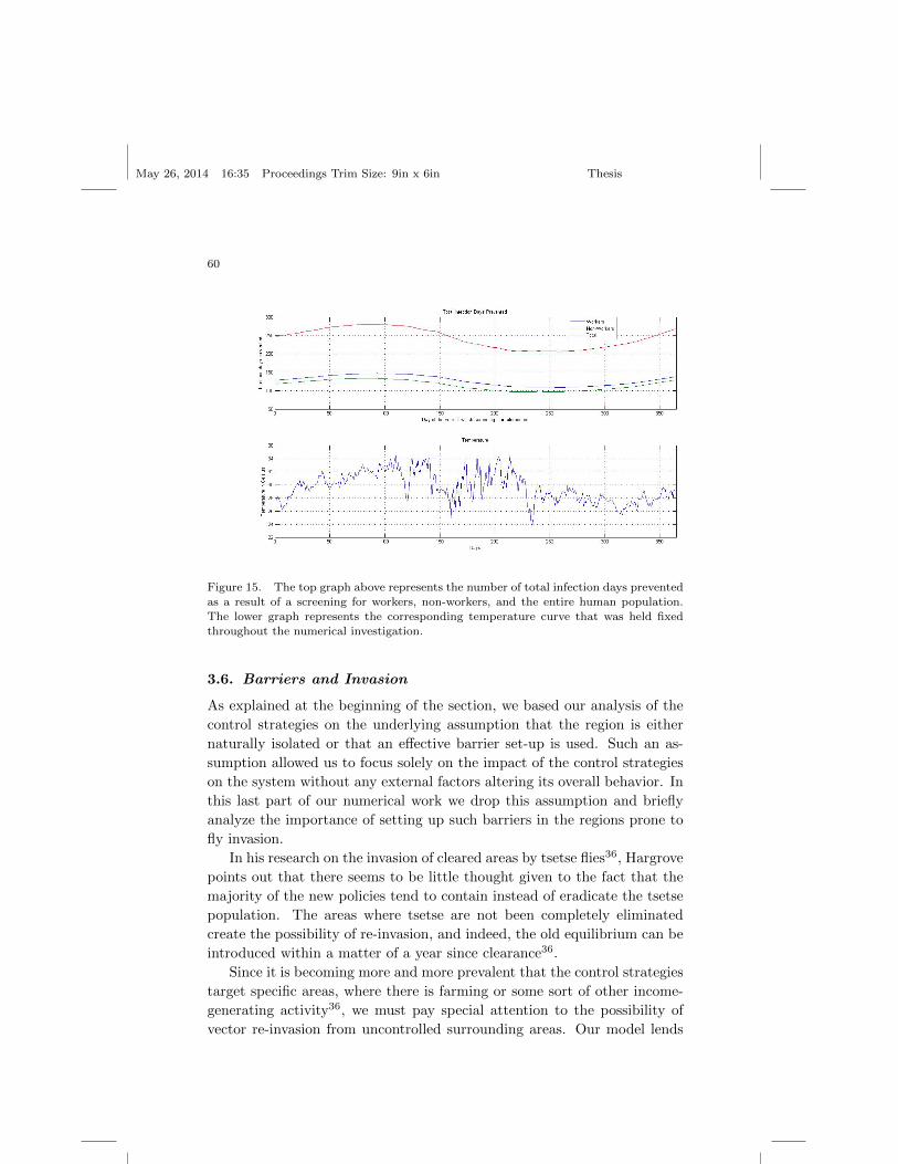
May 26, 2014 16:35 Proceedings Trim Size: 9in x 6in Thesis
60
Figure 15. The top graph above represents the number of total infection days prevented
as a result of a screening for workers, non-workers, and the entire human population.The lower graph represents the corresponding temperature curve that was held fixed
throughout the numerical investigation.
3.6. Barriers and Invasion
As explained at the beginning of the section, we based our analysis of the
control strategies on the underlying assumption that the region is either
naturally isolated or that an effective barrier set-up is used. Such an as-
sumption allowed us to focus solely on the impact of the control strategies
on the system without any external factors altering its overall behavior. In
this last part of our numerical work we drop this assumption and briefly
analyze the importance of setting up such barriers in the regions prone to
fly invasion.
In his research on the invasion of cleared areas by tsetse flies36, Hargrove
points out that there seems to be little thought given to the fact that the
majority of the new policies tend to contain instead of eradicate the tsetse
population. The areas where tsetse are not been completely eliminated
create the possibility of re-invasion, and indeed, the old equilibrium can be
introduced within a matter of a year since clearance36.
Since it is becoming more and more prevalent that the control strategies
target specific areas, where there is farming or some sort of other income-
generating activity36, we must pay special attention to the possibility of
vector re-invasion from uncontrolled surrounding areas. Our model lends
May 26, 2014 16:35 Proceedings Trim Size: 9in x 6in Thesis
61
itself as such example as it is designed specifically for a village-plantation
module and does not concern itself with alternative control measures, such
as control of large area blocks. Due to insufficient funding this module
is an appropriate and prevalent approach to the control of the disease36.
However, its success is only guaranteed if an appropriate barrier system is
set up and maintained fittingly.
In order to demonstrate the devastating impact of invasion and em-
phasize the importance of barrier set-up, we extend our model to assume
external recruitment rate. The modifications are based on the idea that as
we start to control the local tsetse population, we deviate from the implied
local carrying capacity and the flies from the outer regions begin to migrate
into the controlled area until the implied carrying capacity equilibrium is
re-established. For simplicity, we assume that the vectors are migrating at
a constant rate and from the entirety of the surrounding area. We make
an assumption that a totally cleared area of our size (less than a hundred
square kilometers) has a complete replacement rate of 180 days36. In order
to incorporate the impact of a barrier set-up, we assume that an eight-
kilometer-wide barrier is set with a density of four traps per square kilo-
meter, and effective probability of penetration of 0.00120. Needless to say,
such barrier set-up is very extensive and often barriers will be much smaller.
Nevertheless, for the purposes of demonstration, an optimal approach to
barrier set-up that almost entirely mitigates the impact of re-invasion and
practically assumes isolation is adopted.
For the sake of brevity, we only demonstrate the impact of re-invasion
and the barrier set-up solution for an example of trapping application.
Trapping is applied after 365 days and is in effect for a period of 365 days.
The results are summarized in Figure 16.
Figure 16 provides a clear reason as for why the majority of contempo-
rary researchers emphasize the importance of setting up an effective barrier
system. If external migration is incorporated and no barriers are set up,
the effective eradication achieved through trapping is mitigated completely.
Furthermore, the process of trapping itself is significantly less efficient as
the flies started migrating into the region as soon as the control strategy is
introduced. If, however, a control strategy is implemented when the barri-
ers are set up, the impact of external migration is due to our assumptions,
expectedly, almost completely mitigated.
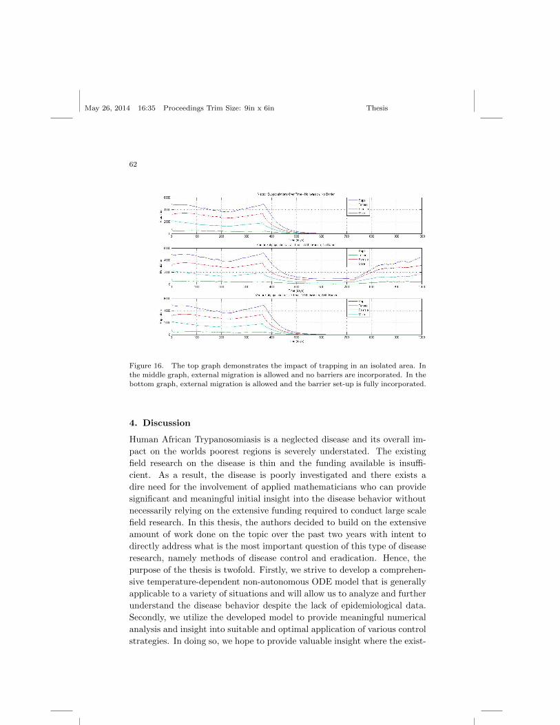
May 26, 2014 16:35 Proceedings Trim Size: 9in x 6in Thesis
62
Figure 16. The top graph demonstrates the impact of trapping in an isolated area. In
the middle graph, external migration is allowed and no barriers are incorporated. In thebottom graph, external migration is allowed and the barrier set-up is fully incorporated.
4. Discussion
Human African Trypanosomiasis is a neglected disease and its overall im-
pact on the worlds poorest regions is severely understated. The existing
field research on the disease is thin and the funding available is insuffi-
cient. As a result, the disease is poorly investigated and there exists a
dire need for the involvement of applied mathematicians who can provide
significant and meaningful initial insight into the disease behavior without
necessarily relying on the extensive funding required to conduct large scale
field research. In this thesis, the authors decided to build on the extensive
amount of work done on the topic over the past two years with intent to
directly address what is the most important question of this type of disease
research, namely methods of disease control and eradication. Hence, the
purpose of the thesis is twofold. Firstly, we strive to develop a comprehen-
sive temperature-dependent non-autonomous ODE model that is generally
applicable to a variety of situations and will allow us to analyze and further
understand the disease behavior despite the lack of epidemiological data.
Secondly, we utilize the developed model to provide meaningful numerical
analysis and insight into suitable and optimal application of various control
strategies. In doing so, we hope to provide valuable insight where the exist-
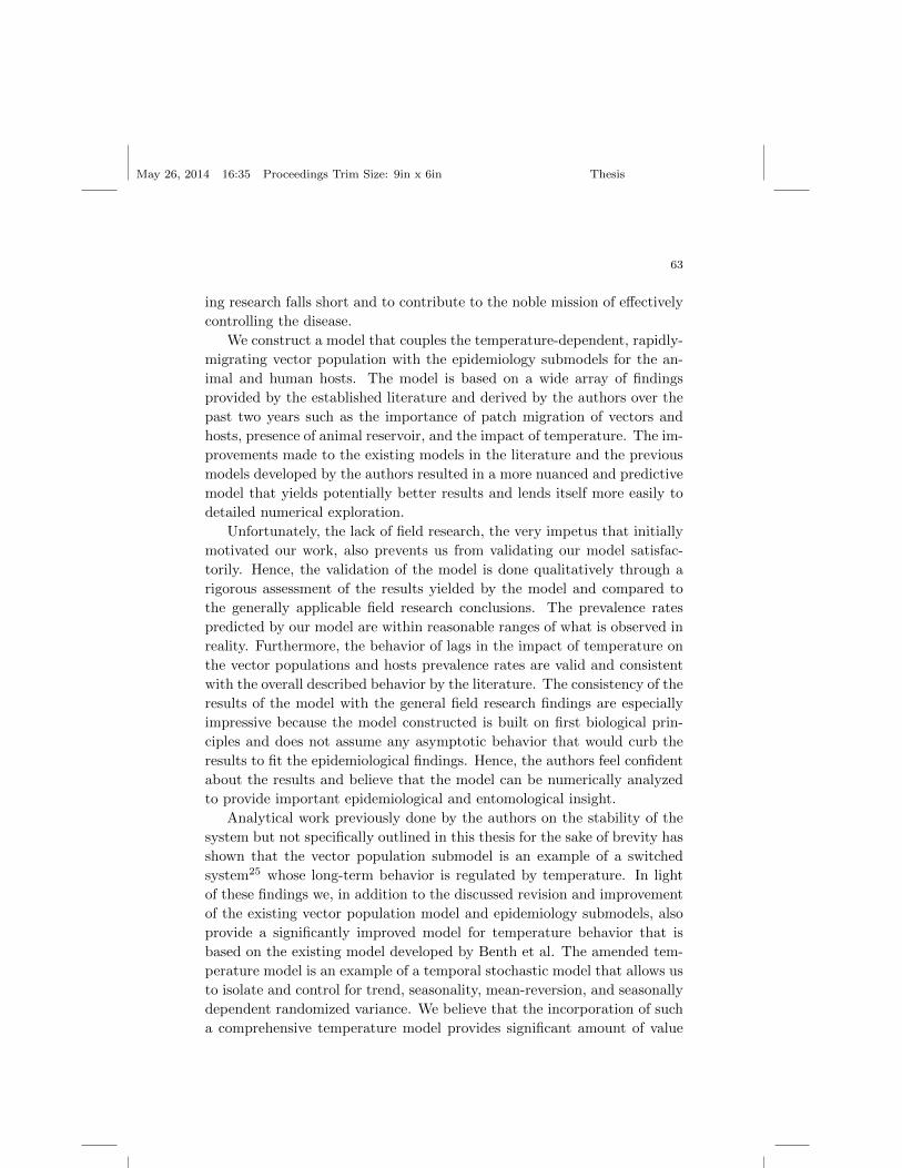
May 26, 2014 16:35 Proceedings Trim Size: 9in x 6in Thesis
63
ing research falls short and to contribute to the noble mission of effectively
controlling the disease.
We construct a model that couples the temperature-dependent, rapidly-
migrating vector population with the epidemiology submodels for the an-
imal and human hosts. The model is based on a wide array of findings
provided by the established literature and derived by the authors over the
past two years such as the importance of patch migration of vectors and
hosts, presence of animal reservoir, and the impact of temperature. The im-
provements made to the existing models in the literature and the previous
models developed by the authors resulted in a more nuanced and predictive
model that yields potentially better results and lends itself more easily to
detailed numerical exploration.
Unfortunately, the lack of field research, the very impetus that initially
motivated our work, also prevents us from validating our model satisfac-
torily. Hence, the validation of the model is done qualitatively through a
rigorous assessment of the results yielded by the model and compared to
the generally applicable field research conclusions. The prevalence rates
predicted by our model are within reasonable ranges of what is observed in
reality. Furthermore, the behavior of lags in the impact of temperature on
the vector populations and hosts prevalence rates are valid and consistent
with the overall described behavior by the literature. The consistency of the
results of the model with the general field research findings are especially
impressive because the model constructed is built on first biological prin-
ciples and does not assume any asymptotic behavior that would curb the
results to fit the epidemiological findings. Hence, the authors feel confident
about the results and believe that the model can be numerically analyzed
to provide important epidemiological and entomological insight.
Analytical work previously done by the authors on the stability of the
system but not specifically outlined in this thesis for the sake of brevity has
shown that the vector population submodel is an example of a switched
system25 whose long-term behavior is regulated by temperature. In light
of these findings we, in addition to the discussed revision and improvement
of the existing vector population model and epidemiology submodels, also
provide a significantly improved model for temperature behavior that is
based on the existing model developed by Benth et al. The amended tem-
perature model is an example of a temporal stochastic model that allows us
to isolate and control for trend, seasonality, mean-reversion, and seasonally
dependent randomized variance. We believe that the incorporation of such
a comprehensive temperature model provides significant amount of value
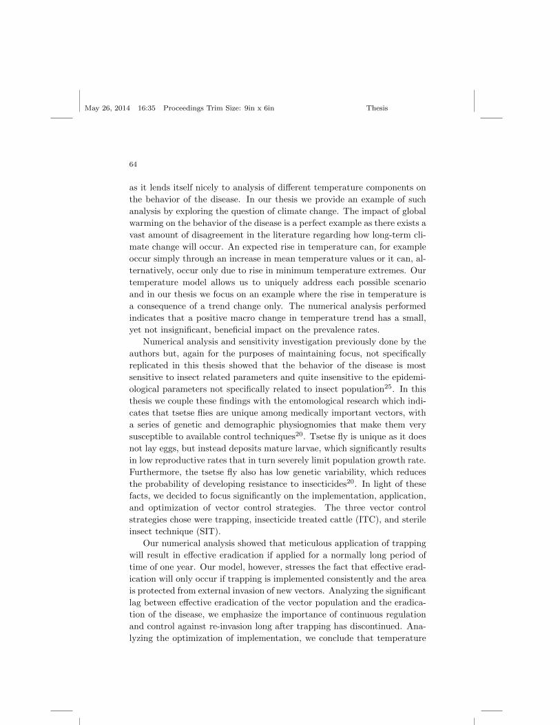
May 26, 2014 16:35 Proceedings Trim Size: 9in x 6in Thesis
64
as it lends itself nicely to analysis of different temperature components on
the behavior of the disease. In our thesis we provide an example of such
analysis by exploring the question of climate change. The impact of global
warming on the behavior of the disease is a perfect example as there exists a
vast amount of disagreement in the literature regarding how long-term cli-
mate change will occur. An expected rise in temperature can, for example
occur simply through an increase in mean temperature values or it can, al-
ternatively, occur only due to rise in minimum temperature extremes. Our
temperature model allows us to uniquely address each possible scenario
and in our thesis we focus on an example where the rise in temperature is
a consequence of a trend change only. The numerical analysis performed
indicates that a positive macro change in temperature trend has a small,
yet not insignificant, beneficial impact on the prevalence rates.
Numerical analysis and sensitivity investigation previously done by the
authors but, again for the purposes of maintaining focus, not specifically
replicated in this thesis showed that the behavior of the disease is most
sensitive to insect related parameters and quite insensitive to the epidemi-
ological parameters not specifically related to insect population25. In this
thesis we couple these findings with the entomological research which indi-
cates that tsetse flies are unique among medically important vectors, with
a series of genetic and demographic physiognomies that make them very
susceptible to available control techniques20. Tsetse fly is unique as it does
not lay eggs, but instead deposits mature larvae, which significantly results
in low reproductive rates that in turn severely limit population growth rate.
Furthermore, the tsetse fly also has low genetic variability, which reduces
the probability of developing resistance to insecticides20. In light of these
facts, we decided to focus significantly on the implementation, application,
and optimization of vector control strategies. The three vector control
strategies chose were trapping, insecticide treated cattle (ITC), and sterile
insect technique (SIT).
Our numerical analysis showed that meticulous application of trapping
will result in effective eradication if applied for a normally long period of
time of one year. Our model, however, stresses the fact that effective erad-
ication will only occur if trapping is implemented consistently and the area
is protected from external invasion of new vectors. Analyzing the significant
lag between effective eradication of the vector population and the eradica-
tion of the disease, we emphasize the importance of continuous regulation
and control against re-invasion long after trapping has discontinued. Ana-
lyzing the optimization of implementation, we conclude that temperature
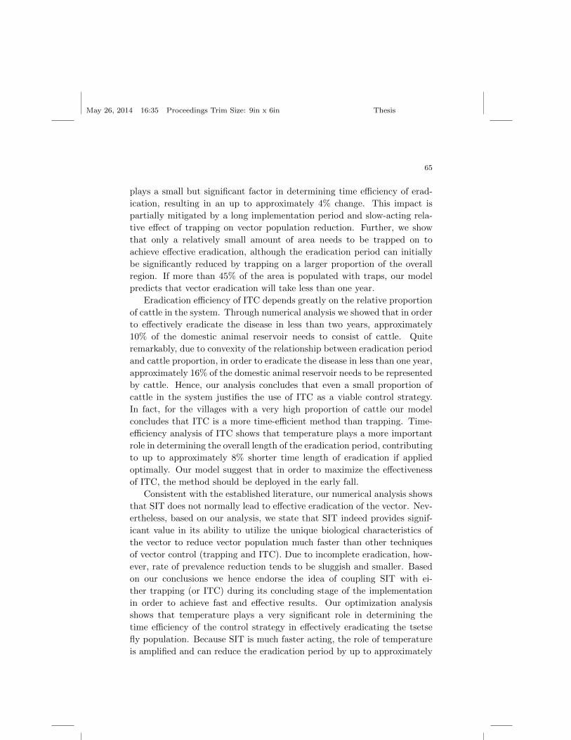
May 26, 2014 16:35 Proceedings Trim Size: 9in x 6in Thesis
65
plays a small but significant factor in determining time efficiency of erad-
ication, resulting in an up to approximately 4% change. This impact is
partially mitigated by a long implementation period and slow-acting rela-
tive effect of trapping on vector population reduction. Further, we show
that only a relatively small amount of area needs to be trapped on to
achieve effective eradication, although the eradication period can initially
be significantly reduced by trapping on a larger proportion of the overall
region. If more than 45% of the area is populated with traps, our model
predicts that vector eradication will take less than one year.
Eradication efficiency of ITC depends greatly on the relative proportion
of cattle in the system. Through numerical analysis we showed that in order
to effectively eradicate the disease in less than two years, approximately
10% of the domestic animal reservoir needs to consist of cattle. Quite
remarkably, due to convexity of the relationship between eradication period
and cattle proportion, in order to eradicate the disease in less than one year,
approximately 16% of the domestic animal reservoir needs to be represented
by cattle. Hence, our analysis concludes that even a small proportion of
cattle in the system justifies the use of ITC as a viable control strategy.
In fact, for the villages with a very high proportion of cattle our model
concludes that ITC is a more time-efficient method than trapping. Time-
efficiency analysis of ITC shows that temperature plays a more important
role in determining the overall length of the eradication period, contributing
to up to approximately 8% shorter time length of eradication if applied
optimally. Our model suggest that in order to maximize the effectiveness
of ITC, the method should be deployed in the early fall.
Consistent with the established literature, our numerical analysis shows
that SIT does not normally lead to effective eradication of the vector. Nev-
ertheless, based on our analysis, we state that SIT indeed provides signif-
icant value in its ability to utilize the unique biological characteristics of
the vector to reduce vector population much faster than other techniques
of vector control (trapping and ITC). Due to incomplete eradication, how-
ever, rate of prevalence reduction tends to be sluggish and smaller. Based
on our conclusions we hence endorse the idea of coupling SIT with ei-
ther trapping (or ITC) during its concluding stage of the implementation
in order to achieve fast and effective results. Our optimization analysis
shows that temperature plays a very significant role in determining the
time efficiency of the control strategy in effectively eradicating the tsetse
fly population. Because SIT is much faster acting, the role of temperature
is amplified and can reduce the eradication period by up to approximately
May 26, 2014 16:35 Proceedings Trim Size: 9in x 6in Thesis
66
25% if introduced at the right time in the year. Examining the relationship
between resource-efficient and time-efficient eradication, we determine that
the agents concerned with time efficiency (e.g. African governments) should
focus more on increasing the number of males released at each interval,
while the agents that are more capital-restricted (e.g. non-governmental
organizations) should reduce the number of males released each time and
instead increase the total number of releases. Our research also further
supports previously made argument that relative time efficiency of SIT is
proportional to the size of the region.
We conclude our investigation of control strategies by analyzing the em-
ployment and optimization of a non-vector control strategy active screening
of the human population. Our analysis further supports the argument made
by our sensitivity study, suggesting that vector control strategies are much
better at disease eradication than the direct epidemiological strategies such
as screening. We show that the implementation of screening cannot lead
to long-term eradication of prevalence rates due to a significant impact
of animal reservoir. This finding directly supports our previous analytical
work done on the topic of host-specific reproduction numbers, which in-
dicated that animal-specific reproduction number is large enough for the
animal reservoir to maintain the infection even if the human population
is removed from the system. Nevertheless, screening implementation does
provide value that vector control strategies lack, as it provides an imme-
diate relief to the infected human population. Due to time and funding
constraints, screening cannot be performed very frequently and the ques-
tion of optimal implementation is hence that much more important. Our
numerical analysis of optimal timing to pilot the programme showed that
the impact of screening can lead to up to approximately 25% change if
implemented at the right time of the year. Our model suggests that the
optimal timing for our specific region is in the spring.
Lastly, we explore, numerically, the impact of re-invasion and the im-
portance of setting up vector population barriers. When re-invasion of flies
is assumed, our standard application of control strategies does not lead to
effective eradication - the relief, as expected, is only temporary. Our anal-
ysis emphazises the importance of setting up a barrier system when the
re-invasion is plausible. Furthermore, the incorporation of invasion possi-
bility into the model allows the future users of the model to control for this
very realistic possibility when exploring the impact of the control strategies.
Moving forward, we remain firm in our belief that a primary purpose
of applied mathematical modeling is to assist with the understanding of
May 26, 2014 16:35 Proceedings Trim Size: 9in x 6in Thesis
67
reality. Hence, one of our hopes is that our model, incorporated with these
control strategies, a stochastic temperature model, and an invasion module,
is to be extended even further and developed into a user-friendly numerical
tool that could help the agencies controlling the disease to make more
informed and efficient decisions. With this idea in mind, our model was
constructed so that it is both general in its function and specific in its
results and can be applied to any local area as long as the suitable adjusting
parameter values are available.
5. Acknowledgments
I would like to thank Professor Dorothy Wallace for her extraordinary sup-
port over the past two years and for her unparalleled guidance, which made
this thesis possible. I would also like to thank my dear friend and colleague
Thomas Madsen with whom I began this journey at the end of our sopho-
more year, who has been involved with this research ever since, and without
whom I would never have gotten to this point. Lastly, I would like to thank
my family - my father Bojan, my mother Magda and my grandparents,
Franci and Mihi - who have been there for me every step of my life and
have guided me to become the person that I am today.
References
1. E. Fevre, B. Wissmann, S. Welburn, and P. Lutumba. Public Library of Sci-ence of Neglected Tropical Diseases 2 12 (2008).
2. C. Nimmo, Travel Medicine and Infectious Disease 8, 263-268 (2010).3. P. Solano, S. Ravel, and T. de Meeus. Trends in Parasitology 26 5, 255-263
(2010).4. McDermott, J.J., and P.G. Coleman, International Journal for Parasitology
31, 603-609 (2001).5. A. Fairlamb, Trends in Parasitology 19 11, 488-494 (2003).6. B. Swallow, Review Paper for PAAT (Programme Against African Trypanoso-
miasis) 1, 1-46 (1999).7. D. Rogers, Parasitology 97, 193-212 (1988).8. J.N. Pollock, Training Manual for Tsetse Control Personnel. Rome: Food and
Agriculture Organization of the United Nations (1982).9. S. Welburn, and I Maudlin, Parasitology Today 15 10, 399-404 (1999).10. S. Funk, H. Nishiura, H. Heesterbeek, W.J. Edmunds, and F. Checchi. PLOS
Computational Biology 9 1 ,(2013).11. K. Chalvet-Monfray, M. Artzrouni, J.-P. Gouteux, P. Auger, and P. Sabatier.
Acta Biologica 46, 207-222 (1998).12. F.E. Benth, J. Saltyte-Benth, and P. Jalinskas. Univ. of Oslo Statistical Re-
search Report 5, 1-28 (2005).
May 26, 2014 16:35 Proceedings Trim Size: 9in x 6in Thesis
68
13. J. Bouyer, F. Stachurski, I. Kabore, B. Bauer, and R. Lancelot. PreventativeVeterinary Medicine 78 223-238 (2007).
14. R. Brun, J. Blum, F. Chappuis, C. Burri The Lancet 375, 148-159 (2009).15. F. Chappuis, L. Loutan, P. Simarro, V. Lejon, and P. Buscher. Clinical Mi-
crobiology Reviews 18 1, 133146 (2005).16. J. Hargrove. Bulletin of Entomological Research 93 19-29 (2003).17. J. Hargrove. Tsetse eradication: sufficiency, necessity and desirability. Re-
search report, DFID Animal Health Programme, Centre for Tropical Veteri-nary Medicine, University of Edinburgh, UK (2003).
18. J. Robays, M. Bilengue, P. Van der Stuyf, and M. Boelaert. Tropical Medicineand International Health 9 5 542-550 (2004).
19. G.A. Vale and S. E. Torr. Medical and Veterinary Entomology 19, 293-305(2005).
20. F.A.S. Kuzoe and C.J. Schofield. Strategic Review of Traps and Targets forTsetse and African Trypanosomiasis Control WHO Special Programme forResearch and Training in Tropical Diseases (2004).
21. D. Rogers and M. Packer, The Lancet 342, 1282-1284 (1993).22. O. Diekmann, J. A. P. Heesterbeek, and M.G. Roberts. J. R. Soc. Interface
7 (2010).23. D. A. Dame and H. R. Ford Entomology Research Division, Agriculture Re-
search Services, United States 213-219 (1968).24. D. A. T. Baldry. Insect Science Applications 1 85-93 (1980).25. T. Madsen, D. Wallace, and N. Zupan BIOMAT International Symposium
2012 (2013).26. M. Artzrouni and J.P. Gouteux. Simulation and Gaming 32 2, 215-227
(2001).27. N. Kon, E. K. N’Goran, I. Sidibe, A.W. Kombassere and J. Bouyer. Medical
and Veterinary Entomology 25, 156-168 (2011).28. S.G.A. Leak, W. Mulatu, E. Authi, G.D.M. d’Ieteren, A.S. Peregrine, G.J.
Rowlands, and J.C.M. Trail. Acta Tropica 53, 121-134 (1993).29. M. Baylis. Acta Tropica 65, 81-96 (1997).30. T. R. Karl, G. Kukla, V. N. Razuvayev, M. J. Changery, R.G. Quayle, R.
R. Heim, D. R. Easterling, and C.B. Fu. Geophysical Research Letters 18 12,2253-2256 (1991).
31. R.D. Dransfield. Insect Science Applications 5 5, 363-368 (1994).32. D. Bourn, I. Grant, A. Shaw, and S. Torr Aspects of Applied Biology 75, 1-12
(2005).33. P.-H. Clausen, I. Adeyemi, B. Bauer , M. Breloeer, F. Salchow and C. Staak
Medical and Veterinary Entomology 12, 169-180 (1998).34. V. A. Dyck, J. Hendrichs, and A. S. Robinson. Sterile Insect Technique:
Principles and Practice in Area-Wide Integrated Pest Management Springer(2005).
35. W. Takken and M. Weiss IAEA Bulletin 20 3, 20-24.36. J.W. Hargrove Bulletin of Entomological Research 90, 201-209 (2000).