semiparametric trending panel data models with cross-sectional dependence€¦ · ·...
TRANSCRIPT

The University of Adelaide School of Economics
Research Paper No. 2010-10 May 2010
Semiparametric Trending Panel Data Models with Cross-Sectional Dependence
Jia Chen, Jiti Gao, and Degui Li

Semiparametric Trending Panel Data Models
with Cross-Sectional Dependence
By Jia Chen, Jiti Gao and Degui Li1
School of Economics, The University of Adelaide, Adelaide, Australia
Abstract
A semiparametric fixed effects model is introduced to describe the nonlinear trending
phenomenon in panel data analysis and it allows for the cross–sectional dependence in
both the regressors and the residuals. A semiparametric profile likelihood approach based
on the first–stage local linear fitting is developed to estimate both the parameter vector
and the time trend function. As both the time series length T and the cross–sectional size
N tend to infinity simultaneously, the resulting semiparametric estimator of the parame-
ter vector is asymptotically normal with a rate of convergence of OP
(1√NT
). Meanwhile,
an asymptotic distribution for the estimate of the nonlinear time trend function is also es-
tablished with a rate of convergence of OP
(1√NTh
). Two simulated examples are provided
to illustrate the finite sample behavior of the proposed estimation method. In addition,
the proposed model and estimation method is applied to the analysis of two sets of real
data.
JEL classification: C13, C14, C23.
Keywords: Cross–sectional dependence, nonlinear time trend, panel data, profile likeli-
hood, semiparametric regression.
Abbreviated title: Semiparametric trending regression
1Corresponding Author: Dr Degui Li, School of Economics, The University of Adelaide, Adelaide SA
5005, Australia. Email: [email protected]
2

1. Introduction
Modeling time series with trend functions has attracted an increasing interest in recent
years. Mainly due to the limitation and practical inapplicability of parametric trend
functions, recent literature focuses on estimating time–varying coefficient trend functions
using nonparametric estimation methods. Such studies include Robinson (1989) and Cai
(2007). Phillips (2001) provides a review on the current development and future directions
about modeling time series with trends. In the meantime, some other nonparametric and
semiparametric models are also developed to deal with time series with a trend function.
Gao and Hawthorne (2006) propose using a semiparametric time series model to address
the issue of whether the trend of a temperature series should be parametrically linear
while allowing for the inclusion of some explanatory variables in a parametric component.
While there is a rich literature on parametric and nonparametric time–varying coef-
ficient time series models, as far as we know, few work has been done in identifying and
estimating the trend function in a panel data model. Atak, Linton and Xiao (2009) pro-
pose a semiparametric panel data model to deal with the modeling of climate change in
the United Kingdom. The authors consider using a model with a dummy variable in the
parametric component while allowing for the time trend function to be nonparametrically
estimated. More recently, Li, Chen and Gao (2010) extend the work of Cai (2007) in a
trending time–varying coefficient time series model to a panel data time–varying coeffi-
cient model. In such existing studies, the residuals are assumed to be cross–sectionally
independent. A recent work by Robinson (2008) may be among the first to introduce a
nonparametric trending time–varying model for the panel data case under cross–sectional
dependence.
In order to take into account of existing information and contribution from a set of
explanatory variables, this paper proposes extending the nonparametric model by Robin-
son (2008) to a semiparametric partially linear panel data model with cross–sectional
dependence. In our discussion, both the residuals and explanatory variables are allowed
to be cross–sectionally dependent.
The model we consider in this paper is a semiparametric trending panel data model
of the form
Yit = X>it β + ft + αi + eit, (1.1)
Xit = gt + vit, i = 1, · · · , N, t = 1, · · · , T, (1.2)
3

where β is a d–dimensional vector of unknown parameters, ft = f(tT
)and gt = g
(tT
)are both time trend functions with f(·) and g(·) being unknown, both {eit} and {vit}are independent and identically distributed (i.i.d.) across time but correlated among
individuals, and αi are fixed effects satisfying
N∑i=1
αi = 0. (1.3)
Note that {αi} is allowed to be correlated with {Xit} through some unknown structure,
while {eit} is assumed to be independent of {vit}.
Models (1.1) and (1.2) cover and extend some existing models. When β = 0, model
(1.1) reduces to the nonparametric model discussed in Robinson (2008). When N = 1,
models (1.1) and (1.2) reduce to the models discussed in Gao and Hawthorne (2006).
Meanwhile, model (1.2) allows for {Xit} to have a trend function and thus be nonsta-
tionary. As a consequence, models (1.1) and (1.2) become more applicable in practice
than some of the existing models discussed in Cai (2007), and Li, Chen and Gao (2010),
in which {Xit} is assumed to be stationary. Such practical situations include the model-
ing of the dependence between the share consumption, {Yit}, on the total consumption,
{Xit}, as well as the modeling of the dependence of the mean temperature series, {Yit},on the Southern Oscillation Index, {Xit}. Furthermore, we relax the cross–sectional in-
dependence assumption on both the regressors {Xit} and the error process {eit}. As
pointed out in Chapter 10 of Hsiao (2003), this makes panel data models more practically
applicable because there is no natural ordering for cross–sectional indices. As a result,
appropriate modeling and estimation of cross–sectional correlatedness becomes difficult
particularly when the dimension of cross–sectional observation N is large. To be able to
study the asymptotic theory of our proposed estimation method in this paper, we will
impose certain mild moment conditions on {eit} and {vit} as in (3.1)–(3.3) in Section 3.
The main objective of this paper is then to construct a consistent estimation method
for the parameter vector β and the trending function f(·). Throughout the paper, both
the time series length T and the cross sections size N are allowed to tend to infinity. A
semiparametric dummy–variable based profile likelihood estimation method is developed
to estimate both β and f(·) based on first–stage local linear fitting. The resulting estima-
tor of β is shown to be asymptotically normal with a rate of convergence of OP
(1√NT
).
Meanwhile, an asymptotic distribution for the nonparametric estimate of the time trend
4

function is also established with a rate of convergence of OP
(1√NTh
). In addition, we also
propose a semiparametric estimator for the cross–sectional covariance matrix of {vit, eit},which is useful in constructing the confidence intervals of the estimator of β and estimate
of f(·).
The rest of the paper is organized as follows. A semiparametric pooled profile like-
lihood method for β and f(·) is proposed in Section 2. The asymptotic theory of the
proposed estimation method is established in Section 3. Some related discussions, such
as estimation of some covariance matrices, an averaged profile likelihood estimator and
the cross–validation bandwidth selection method, are given in Section 4. Two simulated
examples as well as two real–data applications are provided in Section 5. Section 6 con-
cludes the paper. The mathematical proofs of the main results are given in Appendices
A and B.
2. Estimation method
Several existing semiparametric estimation methods can be developed to estimate the
parameter vector β and the time trend function f(·). Among such estimation methods,
the averaged profile likelihood estimation method is a commonly–used method and has
been investigated by some authors in both the time series and panel data cases (see, for
example, Fan and Huang 2005; Su and Ullah 2006; Atak, Linton and Xiao 2009). As we
discuss in Section 4.3, the averaged profile likelihood estimation method is not so efficient
for our semiparametric setting. Thus, we propose using a semiparametric pooled profile
likelihood method associated with a dummy variable to estimate β and f(·).
Before we propose the estimation method, we need to introduce the following notation:
Y = (Y11, · · · , Y1T , Y21, · · · , Y2T , YN1, · · · , YNT )>,
X = (X11, · · · , X1T , X21, · · · , X2T , XN1, · · · , XNT )>,
α = (α2, · · · , αN)>, D = (−iN−1, IN−1)> ⊗ iT ,
f = iN ⊗ (f1, · · · , fT )>, e = (e11, · · · , e1T , e21, · · · , e2T , eN1, · · · , eNT )>,
where ik is the k × 1 vector of ones and Ik is the k × k identity matrix. AsN∑i=1
αi = 0,
model (1.1) can be rewritten as
Y = Xβ + f +Dα + e. (2.1)
5

Let K(·) denote a kernel function and h is a bandwidth. Denote Z(τ) =
1 1−τT
Th
......
1 T−τTTh
and Z(τ) = iN ⊗ Z(τ). Then by Taylor expansion,
f ≈ Z(τ)
f(τ)
hf ′(τ)
.Let W (τ) = diag
(K(1−τT
h), · · · , K
(T−τTTh
))and W (τ) = IN ⊗W (τ). The semipara-
metric dummy–variable based profile likelihood estimation method is proposed as follows.
(i) For given α and β, we estimate f(τ) and f ′(τ) by fα,β(τ)
hf ′α,β(τ)
= arg min(a,b)>
(Y − Xβ −Dα− Z(τ)(a, b)>
)>W (τ)
(Y − Xβ −Dα− Z(τ)(a, b)>
).
If we denote S(τ) =(Z>(τ)W (τ)Z(τ)
)−1Z>(τ)W (τ), then by simple calculation,
we have
fα,β(τ) = (1, 0)S(τ)(Y − Xβ −Dα) = s(τ)(Y − Xβ −Dα), (2.2)
where s(τ) = (1, 0)S(τ).
(ii) Denote
fα,β = iN ⊗(fα,β (1/T ) , · · · , fα,β (T/T )
)>= S(Y − Xβ −Dα),
where S = iN ⊗(s> (1/T ) , · · · , s> (T/T )
)>. Then we estimate α and β by
(α>, β>)> = arg min(α>,β>)>
(Y − Xβ −Dα− fα,β
)> (Y − Xβ −Dα− fα,β
)= arg min
(α>,β>)>
(Y ∗ − X∗β −D∗α
)> (Y ∗ − X∗β −D∗α
). (2.3)
where Y ∗ =(INT − S
)Y , X∗ =
(INT − S
)X and D∗ =
(INT − S
)D.
Define M∗ = INT −D∗(D∗>D∗
)−1D∗>. Simple calculation leads to the solution of
the minimization problem (2.3):
β =(X∗>M∗X∗
)−1X∗>M∗Y ∗, (2.4)
α =(D∗>D∗
)−1D∗>
(Y ∗ − X∗β
). (2.5)
6

(iii) Plug (2.4) and (2.5) into (2.2) to obtain the estimate of f(τ) by
f(τ) = s(τ)(Y − Xβ −Dα
). (2.6)
Note that our study in Sections 3 and 5 below shows that the proposed pooled profile
likelihood method associated with a dummy variable has both theoretical and numerical
advantages over the averaged profile likelihood estimation method.
3. The main results
In this section, we first introduce some regularity assumptions and establish asymptotic
distributions for β and f(·).
3.1. Assumptions
A1. The kernel function K(·) is continuous and symmetric with compact support.
A2. Let vt = (v1t, · · · , vNt)>, 1 ≤ t ≤ T . Suppose that {vt, t ≥ 1} is a sequence of
independent and identically distributed (i.i.d.) N × d random matrices with zero
mean and E[‖vit‖4
]< ∞. There exist d × d positive definite matrices Σv and Σ∗v,
such that as N →∞,
1
N
N∑i=1
E[vitv
>it
]−→ Σv,
1
N
N∑i=1
N∑j=1
E[vitv
>jt
]−→ Σ∗v, E
∥∥∥∥∥N∑i=1
vit
∥∥∥∥∥δ
= O(N δ/2
),
(3.1)
where δ > 2 is a positive constant.
A3. The trend functions f(·) and g(·) have continuous derivatives of up to the second
order.
A4. Let et = {eit, 1 ≤ i ≤ N}. Suppose that {et, t ≥ 1} is a sequence of i.i.d. random
errors with zero mean and independent of {vit}. There exists a d×d positive definite
matrix Σv,e such that as N →∞,
1
N
N∑i=1
N∑j=1
E[vi1v
>j1
]E [ei1ej1]→ Σv,e. (3.2)
Furthermore, there is some 0 < σ2e <∞ such that as N →∞
1
NE
(N∑i=1
eit
)2
→ σ2e and E
∣∣∣∣∣N∑i=1
eit
∣∣∣∣∣δ
= O(N δ/2
), (3.3)
where δ > 2 is as defined in A2.
7

A5. The bandwidth h satisfies as T →∞ and N →∞ simultaneously,
NTh8 → 0,
√NTh
log(NT )→∞ and
T 1− 2δh
log(NT )→∞.
Remark 3.1. A1 is a mild condition on the kernel function and many commonly–used
kernels, including the Epanechnikov kernel, satisfy A1. Furthermore, the compact support
condition for the kernel function can be relaxed at the cost of more technical proofs. In
A2, we impose some moment conditions on {vit} and allow for cross–sectional dependence
of {vit} and thus {Xit}. When {vit} is also i.i.d. across individuals, it is easy to check that
(3.1) holds. Since there is no natural ordering for cross–sectional indices, it may not be
appropriate to impose any kind of mixing or martingale conditions on {vit} when vit and
vjt are dependent. Equation (3.1) instead imposes certain conditions on the measurement
of the ‘distance’ between cross–sections ij and ik. To explain this in some detail, let us
consider the case of d = 1 and define a kind of ‘distance’ function among the cross–sections
of the form
ρ(i1, i2, · · · , ik) = E[vj1i1,1 · · · v
jkik,1
], (3.4)
and then consider one of the cases where k = 4 and j1 = j2 = · · · = j4 = 1. In addition,
we focus on the case where all 1 ≤ i1, i2, · · · , i4 ≤ N are different. Consider a distance
function of the form
ρ(i1, i2, · · · , i4) =1
|i4 − i3|δ3|i3 − i2|δ2 · · · |i2 − i1|δ1(3.5)
for δi > 0 for all 1 ≤ i ≤ 3. In this case, equation (3.1) can be verified because
N∑i1=1
N∑i2=1
· · ·N∑i4=1
E [vi1,1 · · · vi4,1] = O(N4−
∑3
j=1δj)
= O(N2)
(3.6)
when∑3j=1 δj ≥ 2. Obviously, the conventional Euclidean metric is covered. One may
also show that equation (3.1) can also be verified when some other distance functions,
including an exponential distance function, are considered.
A3 is a commonly used condition in local linear fitting. In A2 and A4, we assume
that both {et} and {vt} are i.i.d.. This can be relaxed by allowing both {et} and {vt}to be stationary and α–mixing (see, for example, Gao 2007). In A4, we also do need the
mutual independence between vit and eit in this paper. When vit and eit are dependent
each other, we do not necessarily have E[viteit] = 0. In this case, a modified estimation
8

method, such as an instrumental variable based method may be needed to construct a
consistent estimator for β. To emphasize the main ideas, the proposed estimation method
and the resulting theory as well as to avoid involving further technicality, we establish the
main results under Conditions A1–A5 throughout this paper. However, such extensions
are left for future discussion. The cross–sectional dependence conditions in (3.2) and
(3.3) are similar to those in (3.1). A5 is required for establishing the asymptotic theory
without involving too much technicality. A5 covers the case of NT→ λ for 0 ≤ λ ≤ ∞.
For example, when N is proportional to T , A5 reduces to Th4 → 0 and T1− 2
δ hlog(T )
→∞. For
the case of N = [T c], A5 reduces to T 1+ch8 → 0 and T1− 2
δ hlog(T )
→ ∞ when c ≥ 1 − 4δ
for
δ > 4.
3.2. Asymptotic theory
We first establish an asymptotic distribution for β in the following theorem.
Theorem 3.1. Let Conditions A1–A5 hold. Then as T →∞ and N →∞ simultaneously
√NT
(β − β
)d−→ N
(0d, Σ−1v Σv,eΣ
−1v
). (3.7)
Remark 3.2. The above theorem shows that the proposed pooled profile likelihood
estimator of β can achieve the root–NT convergence rate. As both T and N tend to
infinity jointly, the asymptotic variance in (3.7) is simplified, compared with some existing
literature on the profile likelihood estimation for semiparametric panel data models with
fixed effects (see, for example, Su and Ullah 2006). A consistent estimation method for
Σv and Σv,e will be proposed in Section 4.1 below.
Define µj =∫ujK(u)du and νj =
∫ujK2(u)du. An asymptotic distribution of f(τ) is
established in the following theorem.
Theorem 3.2. Let Conditions A1–A5 hold. Then as T →∞ and N →∞ simultaneously
√NTh
(f(τ)− f(τ)− bf (τ)h2 + oP (h2)
)d−→ N
(0, ν0σ
2e
), (3.8)
where bf (τ) = 12µ2f
′′(τ).
Remark 3.3. The asymptotic distribution in (3.8) is a standard result for local linear
fitting of nonlinear time trend function. From (3.8), we can obtain the mean integrated
square error (MISE) of f(·)
MISE(f(τ)) = E∫ 1
0
(f(τ)− f(τ)
)2dτ ≈ ν0σ
2e
NTh+∫ 1
0b2f (τ)dτ h4, (3.9)
9

where the symbol “an ≈ bn” denotes that anbn→ 1 as n→∞.
From (3.9), we can obtain an optimal bandwidth of the form
hopt =
(ν0σ
2e
4∫ 10 b
2f (τ)dτ
)1/5
(NT )−1/5. (3.10)
The above bandwidth selection method cannot be implemented directly as both σ2e
and b2f (τ) in (3.10) are unknown. Hence, in the simulation study in Section 5, we propose
using a semiparametric “leave–one–out” cross validation method that will be introduced
in Section 4.3 below.
4. Some related discussions
In Section 4.1, consistent estimators are constructed for Σv, Σv,e and σ2e which are
involved in Theorems 3.1 and 3.2. Then, an averaged profile likelihood estimation is
introduced in Section 4.2. The so–called “leave–one–out” cross validation bandwidth
selection criterion is provided in Section 4.3.
4.1. Estimation of Σv, Σv,e and σ2e
To make the proposed estimation method practically implementable, we also need to
construct consistent estimators for Σv and Σv,e. Define
Σv(i) =1
T
T∑t=1
vitv>it and vit = Xit − gt, (4.1)
where gt := g(tT
)is the pooled local linear estimate of g
(tT
). Then, Σv can be estimated
by
Σv =1
N
N∑i=1
Σv(i). (4.2)
By the uniform consistency of the pooled local linear estimate (see the proofs in
Appendix B) and g(·) is independent of i, it is easy to check that Σv(i) is a consistent
estimator of E[vi1v
>i1
]for each i, which implies that Σv is a consistent estimator of Σv.
Let vit be defined as in (4.1) and
eit = Yit −X>it β − ft, (4.3)
where ft := f(tT
). Then, ρij(v) := E
[vi1v
>j1
]and ρij(e) := E [ei1ej1] can be estimated by
ρij(v) =1
T
T∑i=1
vitv>jt and ρij(e) =
1
T
T∑i=1
eite>jt, (4.4)
10

respectively. Let ϕN be some positive integer such that ϕN ≤ N and ϕN →∞.
By (3.2), Σv,e can be consistently estimated by
Σv,e =1
ϕN
ϕN∑i=1
ϕN∑j=1
ρij(v)ρij(e). (4.5)
Similarly, by (3.3), σ2e can be consistently estimated by
σ2e =
1
T
T∑t=1
σ2e(t) and σ2
e(t) =1
ϕN
ϕN∑i=1
ϕN∑j=1
eitejt. (4.6)
Following Theorems 3.1 and 3.2, one may show that the resulting estimators are all
consistent.
4.2. Averaged profile likelihood estimation method
AsN∑i=1
αi = 0, another way to eliminate the individual effects αi from model (1.1) is
to take averages over i
YAt = X>Atβ + ft + eAt, (4.7)
where the subscript A indicates averaging with respect to i, YAt = 1N
N∑i=1
Yit, XAt =
1N
N∑i=1
Xit and eAt == 1N
N∑i=1
eit. Denote YA = (YA1, · · · , YAT )>, XA = (XA1, · · · , XAT )>,
f = (f1, · · · , fT )> and eA = (eA1, · · · , eAT )>. Then, model (4.7) can be rewritten as
YA = XAβ + f + eA. (4.8)
Then, applying the profile likelihood estimation approach to model (4.8), one can
obtain the averaged profile likelihood estimator of β and estimate of f(·) by
βA =(X∗>A X∗A
)−1X∗>A Y ∗A ,
fA(τ) = (1, 0)(Z>(τ)W (t)Z(τ)
)−1Z>(τ)W (t)(YA −XAβA),
where X∗A = XA −MXA = (IT −M)XA, Y ∗A = (IT −M)YA,
M =
(1, 0)
(Z>(1/T )W (1/T )Z(1/T )
)−1Z>(1/T )W (1/T )
...
(1, 0)(Z>(T/T )W (T/T )Z(T/T )
)−1Z>(T/T )W (T/T )
,
in which W (τ) and Z(τ) are defined in Section 2, IT is the T × T identity matrix.
11

It can be shown that the rate of convergence of βA to β is of the order√T , while the
rate of convergence of fA(τ) to f(τ) is of the same order of√NTh as that for f(τ). This
is clearly illustrated in Tables 5.1 and 5.2 below.
4.3. Bandwidth Selection
In this section, we adopt the “leave–one–out” cross validation method to select the
bandwidth for both the pooled and averaged profile likelihood estimation. The selection
procedure can be described as follows.
Let β(−1), α(−1) and f(−1)(·) be the leave–one–out versions of β, α and f(·) in (2.4)–
(2.6), respectively. The leave–one–out estimator of h, hcv, is chosen such that
hcv = arg min1
NT
(Y − Xβ(−1) −
˜f (−1) −Dα(−1)
)T (Y − Xβ(−1) −
˜f (−1) −Dα(−1)
), (4.9)
where˜f (−1) is defined in the same way as f in (2.1) with f(·) being replaced by f(−1)(·).
5. Examples of implementation
We next carry out simulations to compare the small sample behavior of the two profile
likelihood estimation methods: the pooled and the averaged methods. Meanwhile, two
real–data examples are provided to show that our estimation method performs well in
the empirical analysis of a consumer price index data from Australia and a temperature
series data from the United Kingdom. We find significant increasing trends in both of the
data sets.
5.1. Simulated Examples
Example 5.1. Consider one data generating process of the form
Yit = Xitβ + f(t/T ) + αi + eit, 1 ≤ i ≤ N, 1 ≤ t ≤ T, (5.1)
where β = 2, f(u) = u3 + u, αi = 1T
T∑t=1
Xit for i = 1, · · ·, N − 1, and αN = −N−1∑i=1
αi. The
error terms eit are generated as follows. For each 1 ≤ t ≤ T , let e·t = (e1t, ε2t, · · · , eNt),which is a N–dimensional vector. Then, {e·t, 1 ≤ t ≤ T} is generated as a N–dimensional
vector of independent Gaussian variables with zero mean and covariance matrix (cij)N×N ,
where
cij = 0.8|j−i|, 1 ≤ i, j ≤ N. (5.2)
12

From the way eit are generated, it is easy to see that
E(eitejs) = 0 for 1 ≤ i, j ≤ N, t 6= s,
E(eitejt) = 0.8|j−i| for 1 ≤ i, j ≤ N, 1 ≤ t ≤ T.
The above equations imply that {eit} is cross–sectional dependent and time indepen-
dent. The explanatory variables Xit are generated by
Xit = g(t
T
)+ vit, 1 ≤ i ≤ N, 1 ≤ t ≤ T, (5.3)
where g(u) = 2 sin(πu), {vit} is independent of {eit} and is generated in the same way as
{eit} but with a different covariance matrix (dij)N×N , where dij = 0.5|j−i| for 1 ≤ i, j ≤ N .
WithR = 500 replications, we compare the average square–root of mean squared errors
(ASMSE) of the pooled profile likelihood estimator (PPLE) of β and estimate of f(·) with
that of the averaged profile likelihood estimator of β and estimate of f(·) (APLE). For
a p× 1 parameter β = (β1, · · · , βp)> and a nonparametric function f(·) defined on [0, 1],
the ASMSE’s of their estimators β and f(·) are defined as
ASMSE(β) =1
R
R∑r=1
(1
p
p∑l=1
(β(r)l − βl
)2)1/2
, (5.4)
ASMSE(f) =1
R
R∑r=1
(1
T
T∑t=1
(f (r)(t/T )− f(t/T )
)2)1/2
, (5.5)
where β(r)l and f (r)(·) are the estimates of βl and f(·) in the r-th replication for 1 ≤ l ≤ p
and 1 ≤ r ≤ R.
Table 5.1(a). ASMSE for the profile likelihood estimators of β in Example 5.1
N\T 5 10 20 30
5 PPLE 0.2464 (0.1916) 0.1532 (0.1129) 0.1125 (0.0817) 0.0946 (0.0656)
APLE 0.4158 (0.3980) 0.2381 (0.1864) 0.1775 (0.1312) 0.1439 (0.1012)
10 PPLE 0.1860 (0.1407) 0.1387 (0.1055) 0.0973 (0.0673) 0.0747 (0.0543)
APLE 0.3626 (0.2911) 0.2439 (0.1973) 0.2441 (0.1899) 0.1603 (0.1099)
20 PPLE 0.1511 (0.1137) 0.1149 (0.0867) 0.0733 (0.0524) 0.0462 (0.0338)
APLE 0.3257 (0.2562) 0.2237 (0.1692) 0.1709 (0.1228) 0.1680 (0.1281)
30 PPLE 0.1196 (0.0945) 0.1003 (0.0703) 0.0479 (0.0358) 0.0432 (0.0305)
APLE 0.3123 (0.2368) 0.2053 (0.1450) 0.1744 (0.1073) 0.1506 (0.0985)
13

Table 5.1(b). ASMSE for the profile likelihood estimates of f(·) in Example 5.1
N\T 5 10 20 30
5 PPLE 0.5008 (0.2716) 0.3489 (0.1693) 0.2597 (0.1023) 0.2289 (0.0947)
APLE 0.6829 (0.5000) 0.4285 (0.2531) 0.3230 (0.1529) 0.2735 (0.1291)
10 PPLE 0.4318 (0.2124) 0.3101 (0.1414) 0.2306 (0.0943) 0.1910 (0.0751)
APLE 0.6165 (0.3949) 0.4150 (0.2382) 0.3136 (0.1570) 0.2697 (0.1355)
20 PPLE 0.3446 (0.1667) 0.2622 (0.1096) 0.1969 (0.0759) 0.1561 (0.0564)
APLE 0.5199 (0.3338) 0.3651 (0.2052) 0.2895 (0.1479) 0.2628 (0.1530)
30 PPLE 0.2871 (0.1301) 0.2404 (0.0915) 0.1587 (0.0582) 0.1374 (0.0557)
APLE 0.4740 (0.2900) 0.3394 (0.1712) 0.2805 (0.1246) 0.2465 (0.1192)
Tables 5.1(a) and 5.1(b) reveal that the PPLE outperforms the APLE uniformly. We
can further find that an increase in either N or T results in an obvious improvement
in the performances of the PPLE’s of both β and f(·). In contrast, the increase in
N does not necessarily result in the improvement of the performance of the APLE of β,
although the increase in T seems to lead to better performance of the APLE of β (although
this improvement might be slight). This indicates that the APLE can not estimate the
parameter β well for small T .
Example 5.2. Consider another the data generating process of the form
Yit = X>it β + f(t
T
)+ αi + eit, 1 ≤ i ≤ N, 1 ≤ t ≤ T, (5.6)
where β =(1, 1
2, 2)>
, Xit = (Xit,1, Xit,2, Xit,3)>, f(u) = 2u2 + u,
αi = max
{1
T
T∑t=1
Xit,1,1
T
T∑t=1
Xit,2,1
T
T∑t=1
Xit,3,
}, i = 1, · · · , N − 1,
and αN = −N−1∑i=1
αi. Letting e·t = (ε1t, ε2t, · · · , εNt), then we generate {e·t, 1 ≤ t ≤ T}as a N–dimensional vector of Gaussian variables with zero mean and covariance matrix
(c∗ij)N×N , where c∗ij = 2(i−j)2+1
.
The explanatory variables Xit are generated by Xit = g(tT
)+ vit, where
g(u) =(
1 + sin(πu),1
2u, −u
)>, (5.7)
14

and {vit = (vit,1, vit,2, vit,3)> : 1 ≤ i ≤ N, 1 ≤ t ≤ T} satisfies Evit = 0,
E(vitv
>jt
)=
1
(j − i)2 + 1
4 0 0
0 12
0
0 0 1
, 1 ≤ i, j ≤ N, 1 ≤ t ≤ T,
and E(vitv
>js
)= 0 for 1 ≤ i, j ≤ N and s 6= t.
Table 5.2(a). ASMSE for the profile likelihood estimators of β
N\T 5 10 20 30
5 PPLE 0.3785 (0.2036) 0.2537 (0.1221) 0.1723 (0.0819) 0.1336 (0.0690)
APLE 5.2104 (23.9788) 0.5987 (0.3523) 0.3628 (0.1884) 0.2712 (0.1421)
10 PPLE 0.2693 (0.1395) 0.1717 (0.0857) 0.1159 (0.0579) 0.0960 (0.0473)
APLE 5.6469 (19.3887) 0.6227 (0.3878) 0.3696 (0.1997) 0.2710 (0.1421)
20 PPLE 0.1807 (0.0908) 0.1248 (0.0639) 0.0861 (0.0400) 0.0685 (0.0347)
APLE 5.3776 (17.3639) 0.8067 (0.5337) 0.3609 (0.1922) 0.2798 (0.1326)
30 PPLE 0.1533 (0.0756) 0.0976 (0.0486) 0.0709 (0.0327) 0.0555 (0.0284)
APLE 5.0500 (11.6489) 0.6438 (0.3892) 0.3683 (0.1966) 0.2705 (0.1493)
Table 5.2(b). ASMSE for the profile likelihood estimates of f(·)
N\T 5 10 20 30
5 PPLE 0.7554 (0.4229) 0.4977 (0.2360) 0.3805 (0.1629) 0.2824 (0.1308)
APLE 6.9920 (46.0699) 0.7909 (0.5229) 0.4888 (0.2523) 0.3812 (0.1824)
10 PPLE 0.5457 (0.2773) 0.3846 (0.1709) 0.2762 (0.0994) 0.2406 (0.0783)
APLE 5.4341 (20.3767) 0.7601 (0.4996) 0.4373 (0.2525) 0.3576 (0.1781)
20 PPLE 0.3906 (0.1805) 0.2900 (0.1190) 0.2212 (0.0842) 0.2035 (0.0538)
APLE 6.0141 (22.3286) 0.9452 (0.7246) 0.4360 (0.2441) 0.3475 (0.1749)
30 PPLE 0.3290 (0.1477) 0.2919 (0.0977) 0.2073 (0.0553) 0.1796 (0.0422)
APLE 5.5615 (17.4042) 0.6778 (0.4486) 0.3916 (0.2400) 0.2902 (0.1797)
15

The ASMSE’s of the proposed pooled profile likelihood estimators and the averaged
profile likelihood estimators of β and f(·) are calculated over 500 realizations. The results
for the estimator of β and estimate of f(·) are given in Tables 5.2(a) and 5.2(b), respec-
tively. While one may draw the same conclusions as those from Tables 5.1(a) and 5.1(b):
The PPLE performs uniformly better than the APLE and its performance improves as
either N or T increases, the performance of the APLE for the case of T = 5 is much worse
than that for the PPLE in each individual case. This is mainly because the cross–sectional
dependence imposed in Example 5.2 is stronger than that imposed in Example 5.1.
5.2. An application in modeling consumer price index
This data set consists of the quarterly consumer price index (CPI) numbers of 11
classes of commodities for 8 Australian capital cities spanning from 1994 to 2008 (available
from the Australian Bureau of Statistics at www.abs.gov.au). Here we study the empirical
relationship between the log food CPI and the log all–group CPI. Let Yit be the log food
CPI and Xit be the log all–group CPI for city i at time t, where 1 ≤ i ≤ 8 and 1 ≤ t ≤ 60.
We then assume that {(Yit, Xit)} satisfies a pair of semiparametric models of the form
Yit = Xitβ + ft + αi + eit,
Xit = gt + vit, 1 ≤ i ≤ 8, 1 ≤ t ≤ 60, (5.8)
where αi are individual effects, and both ft and gt are the trend functions.
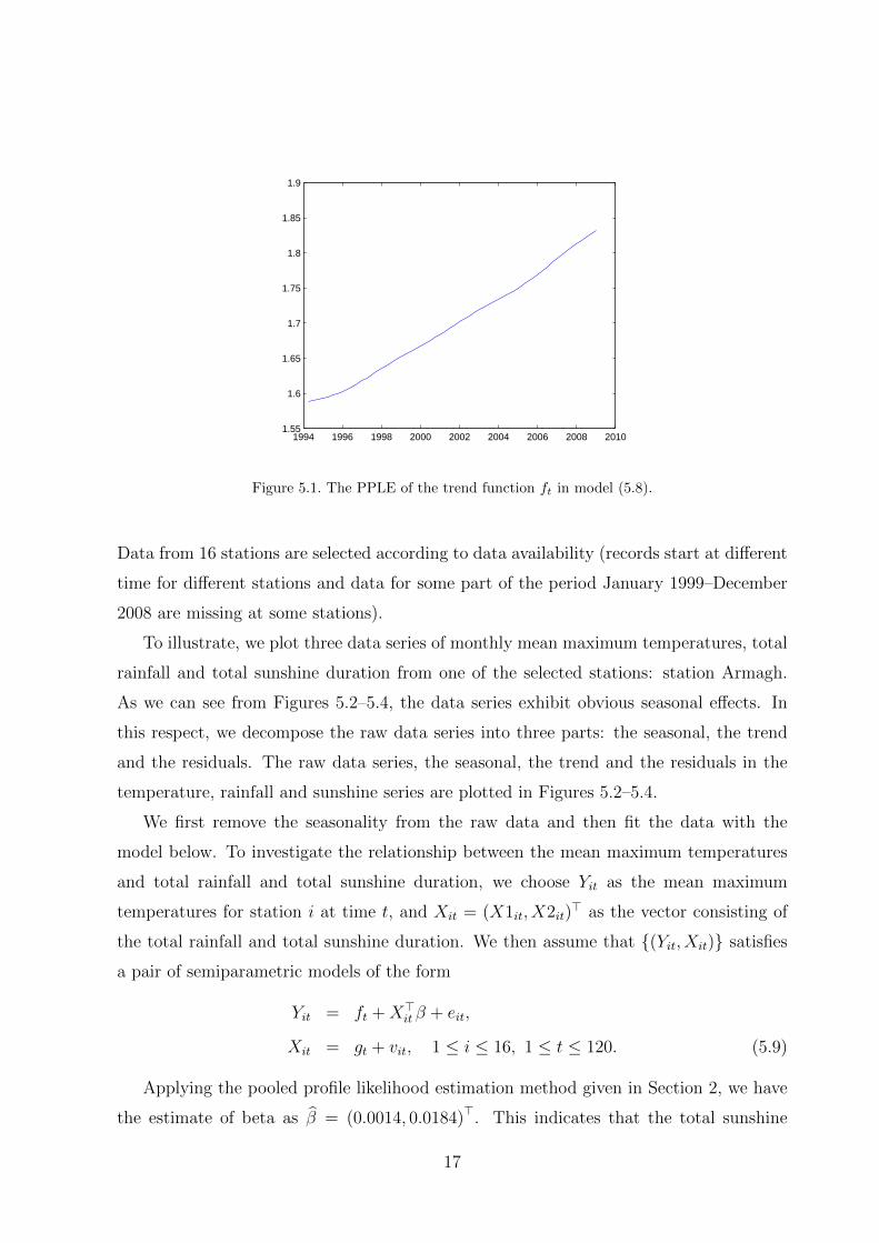
By applying the proposed pooled profile likelihood estimation procedure to the above
data set, we have the estimate for β: β = 0.6617. The estimate of the trend function is
given in Figure 5.1. It follows from this figure that there is a significant upward trend in
ft, which is consistent with the observation that the food CPI series for each city generally
increases with time.
5.3 Trend modeling of a climatic data set
The second data set contains monthly mean maximum temperatures (in Celsius de-
grees), mean minimum temperatures (in Celsius degrees), total rainfall (in millimeters)
and total sunshine duration (in hours) from 37 stations covering the United Kingdom
(available from the UK Met Office at www.metoffice.gov.uk/climate/uk/stationdata). We
use monthly data from January 1999–December 2008 to see if there exists a significant
common trend in the mean maximum temperatures during this period among the stations.
16
1994 1996 1998 2000 2002 2004 2006 2008 20101.55
1.6
1.65
1.7
1.75
1.8
1.85
1.9
Figure 5.1. The PPLE of the trend function ft in model (5.8).
Data from 16 stations are selected according to data availability (records start at different
time for different stations and data for some part of the period January 1999–December
2008 are missing at some stations).
To illustrate, we plot three data series of monthly mean maximum temperatures, total
rainfall and total sunshine duration from one of the selected stations: station Armagh.
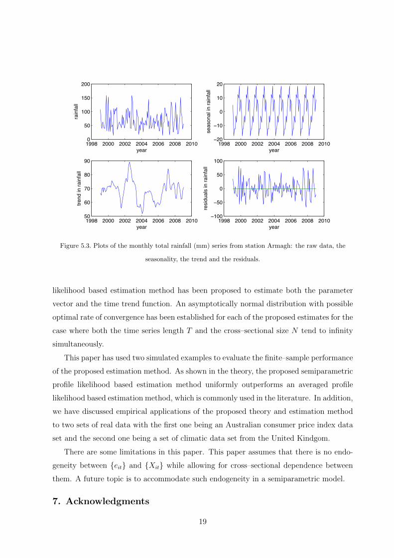
As we can see from Figures 5.2–5.4, the data series exhibit obvious seasonal effects. In
this respect, we decompose the raw data series into three parts: the seasonal, the trend
and the residuals. The raw data series, the seasonal, the trend and the residuals in the
temperature, rainfall and sunshine series are plotted in Figures 5.2–5.4.
We first remove the seasonality from the raw data and then fit the data with the
model below. To investigate the relationship between the mean maximum temperatures
and total rainfall and total sunshine duration, we choose Yit as the mean maximum
temperatures for station i at time t, and Xit = (X1it, X2it)> as the vector consisting of
the total rainfall and total sunshine duration. We then assume that {(Yit, Xit)} satisfies
a pair of semiparametric models of the form
Yit = ft +X>it β + eit,
Xit = gt + vit, 1 ≤ i ≤ 16, 1 ≤ t ≤ 120. (5.9)
Applying the pooled profile likelihood estimation method given in Section 2, we have
the estimate of beta as β = (0.0014, 0.0184)>. This indicates that the total sunshine
17

1998 2000 2002 2004 2006 2008 20105
10
15
20
25
year
Tmax
1998 2000 2002 2004 2006 2008 2010!10
!5
0
5
10
year
seas
onal
in T
max
1998 2000 2002 2004 2006 2008 201012
13
14
15
year
trend
in T
max
1998 2000 2002 2004 2006 2008 2010!4
!2
0
2
4
year
resi
dual
s in
Tm
ax
Figure 5.2. Plots of the monthly mean maximum temperatures (◦C) series from station Armagh: the
raw data, the seasonality, the trend and the residuals.
duration has a more significant influence than the total rainfall on the mean maximum
temperatures.
The estimate of the common trend function ft is plotted in Figure 5.5. Figure 5.5
shows that from the beginning of 1999 to the end of 2000, there is a decrease in the
trend (from about 11.5 at the beginning of 1999 to about 11 at the end of 2000), which
may be a result of an abnormally strong El Nino in 1998 that caused high temperatures
throughout the globe. Then in the two years that followed 1998, the temperatures went
from this extreme down to average. Thereafter, there is an overall increasing trend from
the beginning of 2001 to the end of 2006 (from about 11 at the beginning of 2001 to about
11.8 at the end of 2006). Then from the beginning of 2007 to the end of 2008, there is a
drop in the trend (from about 11.8 at the beginning of 2007 to about 10.5 at the end of
2008), which may be attributed to the La Nina conditions that have a cooling effect on
temperatures.
6. Conclusions and discussion
We have considered a semiparametric fixed effects panel data model with cross–
sectional dependence in both the regressors and the residuals. A semiparametric profile
18
!""# $%%% $%%$ $%%& $%%' $%%# $%!%%
(%
!%%
!(%
$%%
)*+,
,+-./+00
!""# $%%% $%%$ $%%& $%%' $%%# $%!%!$%
!!%
%
!%
$%
)*+,
1*+12.+03-.3,+-./+00
!""# $%%% $%%$ $%%& $%%' $%%# $%!%(%
'%
4%
#%
"%
)*+,
5,*.63-.3,+-./+00
!""# $%%% $%%$ $%%& $%%' $%%# $%!%!!%%
!(%
%
(%
!%%
)*+,
,*1-67+013-.3,+-./+00
Figure 5.3. Plots of the monthly total rainfall (mm) series from station Armagh: the raw data, the
seasonality, the trend and the residuals.
likelihood based estimation method has been proposed to estimate both the parameter
vector and the time trend function. An asymptotically normal distribution with possible
optimal rate of convergence has been established for each of the proposed estimates for the
case where both the time series length T and the cross–sectional size N tend to infinity
simultaneously.
This paper has used two simulated examples to evaluate the finite–sample performance
of the proposed estimation method. As shown in the theory, the proposed semiparametric
profile likelihood based estimation method uniformly outperforms an averaged profile
likelihood based estimation method, which is commonly used in the literature. In addition,
we have discussed empirical applications of the proposed theory and estimation method
to two sets of real data with the first one being an Australian consumer price index data
set and the second one being a set of climatic data set from the United Kindgom.
There are some limitations in this paper. This paper assumes that there is no endo-
geneity between {eit} and {Xit} while allowing for cross–sectional dependence between
them. A future topic is to accommodate such endogeneity in a semiparametric model.
7. Acknowledgments
19

!""# $%%% $%%$ $%%& $%%' $%%# $%!%%
!%%
$%%
(%%
)*+,
-./-01/*
!""# $%%% $%%$ $%%& $%%' $%%# $%!%!!%%
!2%
%
2%
!%%
)*+,
-*+-3/+451/5-./-01/*
!""# $%%% $%%$ $%%& $%%' $%%# $%!%"%
!%%
!!%
!$%
!(%
)*+,
6,*/751/5-./-01/*
!""# $%%% $%%$ $%%& $%%' $%%# $%!%!!%%
!2%
%
2%
!%%
)*+,
,*-17.+4-51/5-./-01/*
Figure 5.4. Plots of the monthly total sunshine duration (hr) series from station Armagh: the raw data,
the seasonality, the trend and the residuals.
1999 2000 2001 2002 2003 2004 2005 2006 2007 2008 200910
10.5
11
11.5
12
Figure 5.5. The PPLE of the trend function ft in model (5.9).
The authors acknowledge the financial support from the Australian Research Council
Discovery Grants Program under Grant Number: DP0879088. Thanks also go to Dr Alev
Atak for providing us with information about the UK temperature data set.
Appendix A: Proofs of the main results
Let C is a generic positive constant whose value may vary from place to place throughout
the rest of this paper.
20

Proof of Theorem 3.1. Note that
β − β =(X∗>M∗X∗
)−1X∗>M∗Y ∗ − β
=(X∗>M∗X∗
)−1X∗>M∗
(INT − S
) (Xβ + f +Dα+ e
)− β
=(X∗>M∗X∗
)−1X∗>M∗f∗ +
(X∗>M∗X∗
)−1X∗>M∗D∗α
+(X∗>M∗X∗
)−1X∗>M∗e∗ (A.1)
=: ΠNT (1) + ΠNT (2) + ΠNT (3),
where f∗ =(INT − S
)f and e∗ =
(INT − S
)e.
AsN∑i=1
αi = 0, we have
ΠNT (2) =(X∗>M∗X∗
)−1X∗>M∗D∗α
=(X∗>M∗X∗
)−1X∗>D∗α−
(X∗>M∗X∗
)−1X∗>D∗
(D∗>D∗
)−1D∗>D∗α
=(X∗>M∗X∗
)−1X∗>D∗α−
(X∗>M∗X∗
)−1X∗>D∗α = 0d, (A.2)
where 0d is a d× 1 vector of zeros.
The asymptotic distribution in Theorem 3.1 can be proved via the following two propositions.
Proposition A.1. Under A1–A3 and A5, we have
ΠNT (1) = oP((NT )−1/2
).
Proof. Note that X∗>M∗X∗ = X∗>X∗ + X∗>D∗(D∗>D∗
)−1D∗>X∗. Hence, to prove Propo-
sition A.1, it suffices for us to prove
1
NTX∗>X∗ = Σv + oP (1), (A.3)
1
NTX∗>D∗
(D∗>D∗
)−1D∗>X∗ = oP (1), (A.4)
X∗>M∗f∗ = oP (√NT ). (A.5)
Step (i). Proof of (A.3). By the definition of X∗, we have
1
NTX∗>X∗ =
1
NTX>
(INT − S
)> (INT − S
)X
=1
NT
N∑i=1
T∑t=1
(Xit − X>s>
(t
T
))(Xit − X>s>
(t
T
))>
=1
NT
N∑i=1
T∑t=1
vitv>it +
1
NT
N∑i=1
T∑t=1
(gt − X>s>
(t
T
))v>it
21

+1
NT
N∑i=1
T∑t=1
vit
(gt − X>s>
(t
T
))>
+1
T
T∑t=1
(gt − X>s>
(t
T
))(gt − X>s>
(t
T
))>=: Π∗NT (1) + Π∗NT (2) + Π∗NT (3) + Π∗NT (4). (A.6)
We first consider Π∗NT (1). Note that
Π∗NT (1) =1
NT
N∑i=1
T∑t=1
vitv>it =
1
T
T∑t=1
(1
N
N∑i=1
vitv>it
)
=1
T
T∑t=1
(1
N
N∑i=1
vitv>it − E
[1
N
N∑i=1
vitv>it
])+
1
T
T∑t=1
E
[1
N
N∑i=1
vitv>it
]=: Π∗NT (1, 1) + Π∗NT (1, 2). (A.7)
By A2 and the Markov inequality, we have, for any ε > 0,
P {|Π∗NT (1, 1)| > ε} ≤ 1
ε2E [Π∗NT (1, 1)]2
=1
ε2T 2
T∑t=1
Var
(1
N
N∑i=1
vitv>it
)=
1
ε2TN2Var
(N∑i=1
vitv>it
)= O
(1
T
).
Hence, as T →∞, we have
Π∗NT (1, 1) = oP (1). (A.8)
By A2, it is easy to check that
Π∗NT (1, 2) = Σv + oP (1) (A.9)
as N,T →∞ simultaneously. By (A.7)–(A.9), we have
Π∗NT (1) = Σv + oP (1). (A.10)
For Π∗NT (4), we use the uniform consistency result
sup0<τ<1
∥∥∥g(τ)− X>s>(τ)∥∥∥ = OP
h2 +
√log(NT )
NTh
. (A.11)
The detailed proof of (A.11) will be given in Appendix B. From (A.11), it is easy to show
Π∗NT (4) = oP (1). (A.12)
By (A.10), (A.12) and the Cauchy–Schwarz inequality,
Π∗NT (2) = oP (1) and Π∗NT (3) = oP (1). (A.13)
With (A.6), (A.10), (A.12) and (A.13), we have shown that (A.3) holds.
22

Step (ii). Proof of (A.4). As SD = 0, we have
D∗>D∗ = D>(INT − S
)> (INT − S
)D = D>D. (A.14)
Furthermore,
D>D =
2T T · · · T
T 2T · · · T
...... · · ·
...
T T · · · 2T
=
T T · · · T
T T · · · T
...... · · ·
...
T T · · · T
+ diag(T, · · · , T ). (A.15)
Letting A = diag(T, · · · , T ), B = (1, · · · , 1)>, C = T and P = (1, · · · , 1), and applying the
result about the inverse matrix (Poirier 1995):
(A+BCP )−1 = A−1 −A−1B(PA−1B + C−1
)−1PA−1,
we have
(D∗>D∗
)−1=(D>D
)−1=
1T −
1NT − 1
NT · · · − 1NT
− 1NT
1T −
1NT · · · − 1
NT
...... · · ·
...
− 1NT − 1
NT · · · 1T −
1NT
. (A.16)
Meanwhile, by the definition of X∗ and D∗ we have
X∗>D∗ = X∗>D = (AT (2), · · · , AT (N)) , (A.17)
where AT (k) = −T∑t=1
X1t +T∑t=1
Xkt = −T∑t=1
v1t +T∑t=1
vkt, k ≥ 2.
By (A.16) and (A.17), we then have
1
NTX∗>D∗
(D∗>D∗
)−1D∗>X∗ =
1
NT
(N∑k=2
A∗T (k)A>T (k)
)
=1
N
N∑k=2
(1
TAT (k)
)(1
TA>T (k)
)−(
1
N
N∑k=2
1
TAT (k)
)(1
N
N∑k=2
1
TA>T (k)
),
where A∗T (k) = 1TAT (k)− 1
NT
N∑k=2
AT (k).
Following the proof of (A.11) in Appendix B, we can show that for each k,
1
TAT (k)
P−→ 0 as T →∞,
which implies ∥∥∥∥ 1
NTX∗>D∗
(D∗>D∗
)−1D∗>X∗
∥∥∥∥ = oP (1).
23

Hence, (A.4) holds.
Step (iii). Proof of (A.5). Note that
X∗>M∗f∗ = X∗>f∗ − X∗>D∗(D∗>D∗
)−1D∗>f∗.
Similarly to the proofs of (A.3) and (A.4), we can show that the leading term on the right
hand side of the above equation is X∗>f∗. Hence, to prove (A.5), we need only to show
X∗>f∗ = oP (√NT ). (A.18)
By the definition of X∗ and f∗, we have
X∗>f∗ =N∑i=1
T∑t=1
(Xit − X>s>
(t
T
))(f
(t
T
)− s
(t
T
)f
)
=N∑i=1
T∑t=1
(vit +
[g
(t
T
)− X>s>
(t
T
)])(f
(t
T
)− s
(t
T
)f
)
=N∑i=1
T∑t=1
vit
(f
(t
T
)− s
(t
T
)f
)−
N∑i=1
T∑t=1
v>s>(t
T
)(f
(t
T
)− s
(t
T
)f
)
+N∑i=1
T∑t=1
(g
(t
T
)− g>s>
(t
T
))(f
(t
T
)− s
(t
T
)f
)=: Π∗NT (5) + Π∗NT (6) + Π∗NT (7), (A.19)
where g = iN ⊗ (g1, g2, · · · , gT )> and v = (v11, · · · , v1T , v21, · · · , v2T , · · · , vNT )>.
Following the argument in the proof of (A.11) in Appendix B and by A2 and A3, we have
sup0<τ<1
∣∣∣f(τ)− s(τ)f∣∣∣ = O
(h2),
sup0<τ<1
∥∥∥g(τ)− g>s>(τ)∥∥∥ = O
(h2),
sup0<τ<1
∥∥∥v>s>(τ)∥∥∥ = OP
√ log(NT )
NTh
,which, together with A5, imply
Π∗NT (5) = OP(√
NTh2)
= oP (√NT ), (A.20)
Π∗NT (6) = OP
(√NT log(NT )h3
)= oP (
√NT ), (A.21)
Π∗NT (7) = OP(NTh4
)= oP (
√NT ). (A.22)
By (A.19)–(A.22), we have shown that (A.18) holds.
In view of (A.3)–(A.5), the proof of Proposition A.1 is completed.
24

Proposition A.2. Let A1–A5 hold. Then we have
√NTΠNT (3)
d−→ N(0d,Σ
−1v Σv,eΣ
−1v
). (A.23)
Proof. To prove (A.23), we need only to show
1
NTX∗>M∗X∗
P−→ Σv (A.24)
and1√NT
X∗>M∗e∗d−→ N (0,Σv,e) . (A.25)
By (A.3) and (A.4) in the proof of Proposition A.1, we can easily obtain (A.24). For the
proof of (A.25), observe that
X∗>M∗e∗ = X∗>e∗ − X∗>D∗(D∗>D∗
)−1D∗>e∗ =: Π∗NT (8)−Π∗NT (9). (A.26)
For Π∗NT (8), we have
1√NT
Π∗NT (8) =1√NT
N∑i=1
T∑t=1
viteit +1√NT
N∑i=1
T∑t=1
(g
(t
T
)− X>s>
(t
T
))eit
− 1√NT
N∑i=1
T∑t=1
vits
(t
T
)e− 1√
NT
N∑i=1
T∑t=1
(g
(t
T
)− X>s>
(t
T
))s
(t
T
)e
=: Π∗NT (10) + Π∗NT (11)−Π∗NT (12)−Π∗NT (13). (A.27)
Following the proof of (A.11) in Appendix B, and by A2, A4 and A5, we have
Π∗NT (11) = OP
h2 +
√log(NT )
NTh
= oP (1), (A.28)
Π∗NT (12) = OP
√ log(NT )
NTh
= oP (1), (A.29)
Π∗NT (13) = OP
√NTh2 +
√log(NT )
NTh
√ log(NT )
NTh
= oP (1). (A.30)
If we can prove
Π∗NT (10)d−→ N (0,Σv,e) , (A.31)
then by (A.28)–(A.30), we will show that
1√NT
Π∗NT (8)d−→ N (0,Σv,e) . (A.32)
As both T and N tend to infinity, we next prove (A.31) by the joint limit approach (see
Phillips and Moon 1999 for example).
25

Letting Zt,N (v, e) = 1√N
N∑i=1
viteit, then Π∗NT (10) can be rewritten as
Π∗NT (10) =1√T
T∑t=1
Zt,N (v, e).
By A2 and A4, {Zt,N (v, e), t ≥ 1} is a sequence of i.i.d. random vectors. Hence, we apply
the Lindeberg–Feller central limit theorem to prove (A.31). For any ε > 0,
1
T
T∑t=1
E(‖Zt,N (v, e)‖2 I
{‖Zt,N (v, e)‖ ≥ ε
√T})
= E(‖Z1,N (v, e)‖2 I
{‖Z1,N (v, e)‖ ≥ ε
√T})→ 0
as N,T → ∞ simultaneously, which implies that the Lindeberg condition is satisfied, which in
turn implies the validity of (A.31).
By (A.16), (A.17) and a standard calculation, we have
Π∗NT (9) =1
T
N∑k=2
AT (k)BT (k)− 1
NT
(N∑k=2
AT (k)
)(N∑k=2
BT (k)
),
where AT (k) =T∑t=1
vkt −T∑t=1
v1t and BT (k) =T∑t=1
ekt −T∑t=1
e1t.
Define AT (k) =T∑t=1
vkt and BT (k) =T∑t=1
ekt for k = 1, · · ·, N . Then,
Π∗NT (9) =1
T
N∑k=2
AT (k)BT (k)− 1
NT
(N∑k=2
AT (k)
)(N∑k=2
BT (k)
)
=1
T
N∑k=2
AT (k)BT (k)− 1
TBT (1)
N∑k=2
AT (k)− 1
TAT (1)
N∑k=2
BT (k)
+N − 1
TAT (1)BT (1)− 1
NT
(N∑k=2
AT (k)
)(N∑k=2
BT (k)
)
+N − 1
NTBT (1)
N∑k=2
AT (k) +N − 1
NTAT (1)
N∑k=2
BT (k)− (N − 1)2
NTAT (1)BT (1)
=1
T
N∑k=2
AT (k)BT (k)− 1
NT
(N∑k=2
AT (k)
)(N∑k=2
BT (k)
)
− 1
NTBT (1)
N∑k=2
AT (k)− 1
NTAT (1)
N∑k=2
BT (k) +N − 1
NTAT (1)BT (1)
=:5∑j=1
Π∗NT (9, j). (A.33)
By A2 and A4, we have, as N,T →∞ simultaneously,
E(Π∗NT (9, 1)Π∗>NT (9, 1)
)26

=1
T 2E
( N∑k=2
T∑t=1
T∑s=1
ektvks
)(N∑k=2
T∑t=1
T∑s=1
ektvks
)>=
1
T 2
T∑t=1
T∑s=1
N∑k1=2
N∑k2=2
E (ek1tek2t)E(vk1sv
>k2s
)
=N∑
k1=2
N∑k2=2
E (ek1,1ek2,1)E(vk1,1v
>k2,1
)= O(N),
E(Π∗NT (9, 2)Π∗>NT (9, 2)
)=
1
N2T 2E
N∑k1=2
T∑t1=1
ek1t1
2
E
N∑k2=2
T∑t2=1
vk2t2
N∑k2=2
T∑t2=1
vk2t2
>
=1
N2T 2
N∑k1=2
N∑j1=2
T∑t1=1
E (ek1t1ej1t1)
N∑k2=2
N∑j2=2
T∑t2=1
E(vk2t2v
>j2t2
)=
1
N2
N∑k1=2
N∑j1=2
E (ek1,1ej1,1)
N∑k2=2
N∑j2=2
E(vk2,1v
>j2,1
) = O(1),
and similarly,
E(Π∗NT (9, 3)Π∗>NT (9, 3)
)= O
(1
N
),
E(Π∗NT (9, 4)Π∗>NT (9, 4)
)= O
(1
N
),
E(Π∗NT (9, 5)Π∗>NT (9, 5)
)= O(1).
Hence,
Π∗NT (9, j) = oP (√NT ), j = 1, · · · , 5. (A.34)
Combining (A.33) and (A.34), we have
Π∗NT (9) = oP (√NT ). (A.35)
By (A.26), (A.32) and (A.35), (A.25) holds. The proof of Proposition A.2 is completed.
Proof of Theorem 3.2. By the definition of f(τ) in (2.6), we have
f(τ)− f(τ) = s(τ)(Y − Xβ −Dα
)− f(τ)
= s(τ)
(INT −D
(D∗>D∗
)−1D∗>(INT − S)
)(Y − Xβ)− f(τ)
=
(s(τ)
(INT −D
(D∗>D∗
)−1D∗>(INT − S)
)f − f(τ)
)+s(τ)
(INT −D
(D∗>D∗
)−1D∗>(INT − S)
)e
+s(τ)
(INT −D
(D∗>D∗
)−1D∗>(INT − S)
)X(β − β)
=: Π∗NT (14) + Π∗NT (15) + Π∗NT (16). (A.36)
27

Note that
s(τ)D = (1, 0)(Z>(τ)W (τ)Z(τ)
)−1Z>(τ)W (τ)D = 0N−1.
Hence, by (A.11) and standard argument for local linear fitting, we have
Π∗NT (14) = s(τ)f − f(τ) =1
2f ′′(τ)µ2h
2 + oP (h2). (A.37)
By the Lindeberg–Feller central limit theorem and following the proof of Proposition A.2,
we have√NThΠ∗NT (15) =
√NThs(τ)e
d−→ N(0, ν0σ2e). (A.38)
By Theorem 3.1, we have
Π∗NT (16) = s(τ)X(β − β) = OP((NT )−1/2
)= oP
((NTh)−1/2
). (A.39)
Hence, by (A.36)–(A.39), we have completed the proof of (3.8).
Appendix B
Proof of (A.11). Note that
g(τ)− X>s>(τ) =(g(τ)− g>s>(τ)
)− v>s>(τ) =: ΞNT,1(τ)− ΞNT,2(τ), (B.1)
where g = iN ⊗ (g1, g2, · · · , gT )>, in which iN is the N × 1 vector of ones.
We now prove
sup0<τ<1
‖ΞNT,2(τ)‖ = OP
√ log(NT )
NTh
, (B.2)
By the definition of s(τ) in Section 2, we have
Ξ>NT,2(τ) = (1, 0)S(τ)v = (1, 0)(Z>(τ)W (τ)Z(τ)
)−1Z>(τ)W (τ)v.
We first prove
sup0<τ<1
∥∥∥∥ 1
NThZ>(τ)W (τ)Z(τ)− Λµ
∥∥∥∥ = O
(1
Th
)= o(1). (B.3)
Note that
1
NThZ>(τ)W (τ)Z(τ) =
1Th
T∑t=1
K(t−τTTh
)1Th
T∑t=1
(t−τTTh
)K(t−τTTh
)1Th
T∑t=1
(t−τTTh
)K(t−τTTh
)1Th
T∑t=1
(t−τTTh
)2K(t−τTTh
) .
By the definition of Riemann integral, we have
1
Th
T∑t=1
(t− τTTh
)jK
(t− τTTh
)= µj +O
(1
Th
),
28

uniformly for 0 < τ < 1.
Hence, (B.3) is proved. In view of (B.3), to prove (B.2), we need only to prove
sup0<τ<1
∥∥∥∥ 1
NThZ>(τ)W (τ)v
∥∥∥∥ = OP
√ log(NT )
NTh
. (B.4)
Note that
1
NThZ>(τ)W (τ)v =
1
NTh
N∑i=1
T∑t=1
K(t−τTTh
)vit
1NTh
N∑i=1
T∑t=1
(t−τTTh
)K(t−τTTh
)vit
.Hence, to prove (B.4), it suffices to show that for j = 0, 1,
sup0<τ<1
∥∥∥∥∥ 1
NTh
N∑i=1
T∑t=1
(t− τTTh
)jK
(t− τTTh
)vit
∥∥∥∥∥ = OP
√ log(NT )
NTh
. (B.5)
Define Qt,N (v) = 1N
N∑i=1
vit. It is easy to see that (B.5) is equivalent to
sup0<τ<1
∥∥∥∥∥ 1
Th
T∑t=1
(t− τTTh
)jK
(t− τTTh
)Qt,N (v)
∥∥∥∥∥ = OP
√ log(NT )
NTh
. (B.6)
Let l(·) be any positive function that satisfies l(n)→∞ as n→∞. Then to prove (B.6), it
suffices to prove
sup0<τ<1
∥∥∥∥∥ 1
Th
T∑t=1
(t− τTTh
)jK
(t− τTTh
)Qt,N (v)
∥∥∥∥∥ = oP
l(NT )
√log(NT )
NTh
. (B.7)
We next cover the interval (0, 1) by a finite number of subintervals {Bl} that are centered
at bl and of length δNT = o(h2). Denoting UNT the number of such subintervals, then UNT =
O(δ−1NT
).
Define Kt,j(τ) = 1Th
(t−τTTh
)jK(t−τTTh
). Observe that
sup0<τ<1
∥∥∥∥∥T∑t=1
Kt,j(τ)Qt,N (v)
∥∥∥∥∥ ≤ max1≤l≤UNT
supτ∈Bl
∥∥∥∥∥T∑t=1
Kt,j(τ)Qt,N (v)−T∑t=1
Kt,j(bl)Qt,N (v)
∥∥∥∥∥+ max
1≤l≤UNT
∥∥∥∥∥T∑t=1
Kt,j(bl)Qt,N (v)
∥∥∥∥∥ =: ΞNT,3 + ΞNT,4. (B.8)
By A1 and taking δNT = O
((l(NT ))1+δ
√log(NT )NTh h2
), we have
ΞNT,3 = OP
(δNTh2
E∥∥∥Q1,N (v)
∥∥∥) = oP
l(NT )
√log(NT )
NTh
. (B.9)
29

For ΞNT,4, we apply the truncation technique. Define
Qt,N (v) = Qt,N (v)I{∥∥∥Qt,N (v)
∥∥∥ ≤ N−1/2T 1/δl(NT )},
Qct,N (v) = Qt,N (v)− Qt,N (v).
Note that
ΞNT,4 ≤ max1≤l≤UNT
∥∥∥∥∥T∑t=1
Kt,j(bl)Qt,N (v)
∥∥∥∥∥+ max1≤l≤UNT
∥∥∥∥∥T∑t=1
Kt,j(bl)Qct,N (v)
∥∥∥∥∥=: ΞNT,5 + ΞNT,6. (B.10)
For ΞNT,6, applying the Markov inequality and A2, we have for any ε > 0,
P
ΞNT,6 > εl(NT )
√log(NT )
NTh
≤ P{
max1≤t≤T
∥∥∥Qct,N (v)∥∥∥ > 0
}
≤T∑t=1
P{∥∥∥Qt,N (v)
∥∥∥ > N−1/2T 1/δl(NT )}
= O
(E∥∥∥Qt,N (v)
∥∥∥δN δ/2(l(NT ))−δ)
= O((l(NT ))−δ
)= o(1),
which implies
ΞNT,6 = oP
l(NT )
√log(NT )
NTh
. (B.11)
For ΞNT,5, observe that∥∥∥Kt,j(bl)Qt,N (v)∥∥∥ ≤ N−1/2T−1+1/δh−1l(NT ).
Applying A2, A5 and Bernstein’s inequality for i.i.d. random variables, we have
P
ΞNT,5 > εl(NT )
√log(NT )
NTh
≤ Cδ−1NT exp
{− ε2(l(NT ))2 log(NT )
C + CεT 1/δ−1/2h−1/2(l(NT ))2(log(NT ))1/2
}(B.12)
≤ Cδ−1NT exp{−M log(NT )} = o(1),
where C > 0 is a constant and M is a sufficiently large positive constant. The second inequality
above holds because of
l(NT )→∞ and(l(NT ))2
T 1/δ−1/2h−1/2(l(NT ))2(log(NT ))1/2→∞.
Hence,
ΞNT,5 = oP
l(NT )
√log(NT )
NTh
. (B.13)
30

From (B.8)–(B.13), we can see that (B.7) holds, which in turn implies the validity of (B.2).
Meanwhile, following standard argument in local linear fitting (see, for example, Fan and
Gijbels 1996), we can show
sup0<τ<1
‖ΞNT,1(τ)‖ = OP(h2). (B.14)
In view of (B.1), (B.2) and (B.14), it has been shown that (A.11) holds.
References
Atak, A., Linton, O., Xiao, Z., 2009. A semiparametric panel model for climate change in the United
Kingdom. Working paper available from http://personal.lse.ac.uk/lintono.
Cai, Z., 2007. Trending time–varying coefficient time series models with serially correlated errors.
Journal of Econometrics 136, 163-188.
Fan, J., Gijbels, I., 1996. Local Polynomial Modelling and Its Applications. Chapman and Hall, London.
Fan, J., Huang, T., 2005. Profile likelihood inferences on semiparametric varying–coefficient partially
linear models. Bernoulli 11, 1031-1057.
Gao, J., 2007. Nonlinear Time Series: Semiparametric and Nonparametric Methods. Chapman &
Hall/CRC, London.
Gao, J., Hawthorne, K., 2006. Semiparametric estimation and testing of the trend of temperature series.
Econometrics Journal 9, 332-355.
Hsiao, C., 2003. Analysis of Panel Data. Cambridge University Press, Cambridge.
Li, D., Chen, J. and Gao, J., 2010. Nonparametric time–varying coefficient panel data models with
fixed effects. Working paper available at http://www.adelaide.edu.au/directory/jiti.gao.
Phillips, P. C. B. and Moon, H., 1999. Linear regression limit theory for nonstationary panel data.
Econometrica 67, 1057-1111.
Poirier, D. J., 1995. Intermediate Statistics and Econometrics: a Comparative Approach. MIT Press,
Boston.
Robinson, P. M., 1989. Nonparametric estimation of time–varying parameters. Statistical Analysis and
Forecasting of Economic Structural Change. Hackl, P. (Ed.). Springer, Berlin, pp. 164-253.
Robinson, P. M., 2008. Nonparametric trending regression with cross-sectional dependence. Working
paper available at http://www.ihs.ac.at/etsast/presentations/Robinson.pdf.
Su, L., Ullah, A., 2006. Profile likelihood estimation of partially linear panel data models with fixed
effects. Economics Letters 92, 75-81.
31