Semiparametric Discriminant Analysisof Mixture Populations

Using Mahalanobis Distance

Probal Chaudhuri and Subhajit Dutta

Indian Statistical Institute, Kolkata.

Workshop on Classification and Regression Trees

Institute of Mathematical Sciences, National University of Singapore

Brief history

Fisher, R. A. (1936), ‘The use of multiplemeasurements in taxonomic problems’,Ann. Eugenics, 7, 179–188.

Fisher was interested in the taxonomicclassification of different species of Iris.He had measurements on the lengths andthe widths of the sepals and the petals ofthe flowers of three different species,namely, Iris setosa, Iris virginica and Irisversicolor.

Brief history (Contd.)

Mahalanobis, P. C. (1936), ‘On thegeneralized distance in statistics’, Proc.Nat. Acad. Sci., India, 12, 49–55.

Mahalanobis met Nelson Annandale atthe 1920 Nagpur session of the IndianScience Congress. Annandale askedMahalanobis to analyze anthropometricmeasurements of Anglo-Indians inCalcutta. This eventually led to thedevelopment of Mahalanobis’ distance.

Mahalanobis’ distance and Fisher’sdiscriminant function

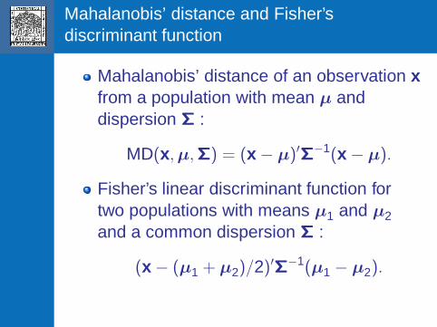
Mahalanobis’ distance of an observation xfrom a population with mean µ anddispersion Σ :

MD(x,µ,Σ) = (x − µ)′Σ−1(x − µ).

Fisher’s linear discriminant function fortwo populations with means µ1 and µ2

and a common dispersion Σ :

(x − (µ1 + µ2)/2)′Σ−1(µ1 − µ2).

Mahalanobis’ distance and Fisher’sdiscriminant function (Contd.)

Mahalanobis’ distance and Fisher’sdiscriminant function (Contd.)

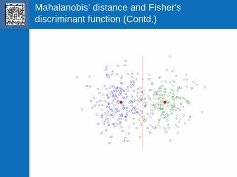
The linear discriminant function hasBayes risk optimality for Gaussian classdistributions which differ in their locationsbut have the same dispersion. This hasbeen discussed in detail in Welch (1939,Biometrika) and Rao (1948, JRSS-B).

In fact, the Bayes risk optimality holds forelliptically symmetric and unimodal classdistributions which differ only in theirlocations.

Examples

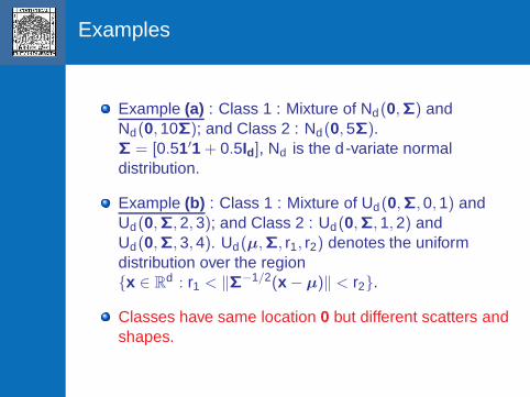
Example (a) : Class 1 : Mixture of Nd(0,Σ) andNd(0,10Σ); and Class 2 : Nd(0,5Σ).Σ = [0.51′1 + 0.5Id], Nd is the d -variate normaldistribution.

Example (b) : Class 1 : Mixture of Ud(0,Σ,0,1) andUd(0,Σ,2,3); and Class 2 : Ud(0,Σ,1,2) andUd(0,Σ,3,4). Ud(µ,Σ, r1, r2) denotes the uniformdistribution over the region{x ∈ R

d : r1 < ‖Σ−1/2(x − µ)‖ < r2}.

Classes have same location 0 but different scatters andshapes.

Bayes class boundaries

−10 −5 0 5 10

−10

−5

05

10

X1

X2

−10 −5 0 5 10

−10

−5

05

10

X1

X2

(a) Example (a)

−4 −2 0 2 4

−4

−2

02

4

X1

X2

−4 −2 0 2 4

−4

−2

02

4

X1

X2

(b) Example (b)

Figure: Bayes class boundaries in R2.

Bayes class boundaries (Contd.)

Class distributions involve ellipticallysymmetric distributions.

They have same location (i.e., 0), and theydiffer in their scatters as well as shapes.

No linear or quadratic classifier will workhere !!

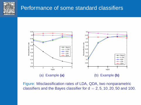
Performance of some standard classifiers

1 2 3 4 50.05

0.1

0.15

0.2

0.25

0.3

0.35

0.4

0.45

0.5

0.55

log(d)

Mis

clas

sific

atio

n ra

te

Bayesk−NNKDELDAQDA

(a) Example (a)

1 2 3 4 50

0.05

0.1

0.15

0.2

0.25

0.3

0.35

0.4

0.45

0.5

log(d)

Mis

clas

sific

atio

n ra

te

Bayesk−NNKDELDAQDA

(b) Example (b)

Figure: Misclassification rates of LDA, QDA, two nonparametricclassifiers and the Bayes classifier for d = 2, 5, 10, 20, 50 and 100.

Nonparametric multinomial additive logisticregression model

Suppose that the class densities are ellipticallysymmetric

fi(x) = |Σi |−1/2gi(‖Σ

−1/2i (x − µi)‖)

= ψi(MD(x,µi ,Σi)) for all i = 1,2.

The class posterior probabilities are

p(1|x) = π1f1(x)/(π1f1(x) + π2f2(x))

andp(2|x) = 1 − p(1|x).

It is easy to see that

log{p(1|x)/p(2|x)} = log(π1f1(x)/π2f2(x)) =

log(π1/π2)+logψ1(MD(x,µ1,Σ1))−logψ2(MD(x,µ2,Σ2)).

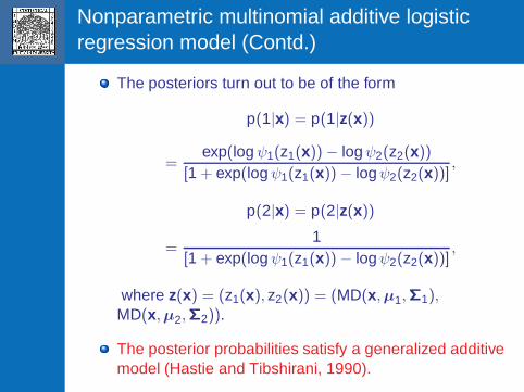
Nonparametric multinomial additive logisticregression model (Contd.)

The posteriors turn out to be of the form

p(1|x) = p(1|z(x))

=exp(logψ1(z1(x))− logψ2(z2(x))

[1 + exp(logψ1(z1(x))− logψ2(z2(x))],

p(2|x) = p(2|z(x))

=1

[1 + exp(logψ1(z1(x))− logψ2(z2(x))],

where z(x) = (z1(x), z2(x)) = (MD(x,µ1,Σ1),MD(x,µ2,Σ2)).

The posterior probabilities satisfy a generalized additivemodel (Hastie and Tibshirani, 1990).

Nonparametric multinomial additive logisticregression model (Contd.)

If we have two normal populations Nd(µ1,Σ) andNd(µ2,Σ), we get linear logistic regression model forthe posterior probabilities. This is related to Fisher’slinear discriminant analysis.

If we have two normal populations Nd(µ1,Σ1) andNd(µ2,Σ2), we get quadratic logistic regression modelfor the posterior probabilities. This is related toquadratic discriminant analysis.

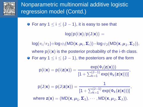
Nonparametric multinomial additive logisticregression model (Contd.)

For any 1 ≤ i ≤ (J − 1), it is easy to see that

log{p(i |x)/p(J|x)} =

log(πi/πJ)+logψi(MD(x,µi ,Σi))−logψJ(MD(x,µJ ,ΣJ)),

where p(i |x) is the posterior probability of the i-th class.

For any 1 ≤ i ≤ (J − 1), the posteriors are of the form

p(i |x) = p(i |z(x)) =exp(Φi(z(x)))

[1 +∑(J−1)

k=1 exp(Φk (z(x)))],

p(J|x) = p(J|z(x)) =1

[1 +∑(J−1)

k=1 exp(Φk (z(x)))],

where z(x) = (MD(x,µ1,Σ1), · · · ,MD(x,µJ ,ΣJ)).

Nonparametric multinomial additive logisticregression model (Contd.)

We replace the original feature variablesby the Mahalanobis’ distances fromdifferent classes.

x → z(x) = (MD(x,µ1,Σ1), · · · ,MD(x,µJ ,ΣJ)).

One can use the backfitting algorithm(Hastie and Tibshirani, 1990) to estimatethe posterior probabilities from the trainingdata.

More general class distributions

Non-elliptic class distributions.

Multi-modal class distributions.

Mixture models for class distributions.

Finite mixture of elliptically symmetric densities

Assume

fi(x) =Ri∑

k=1

θik |Σik |−1/2gik(‖Σ

−1/2ik (x − µik)‖),

where θiks are positive satisfying∑Ri

k=1 θik = 1 for all1 ≤ i ≤ J.The posterior probability for the i-th class is

p(i |x) =Ri∑

r=1

p(cir |x) for all 1 ≤ i ≤ J,

where cir denotes the r -th sub-class in the i-th class.The posterior probability p(cir |x) satisfies a multinomialadditive logistic regression model because thedistribution of the sub-population cir is ellipticallysymmetric.

The missing data problem

In the training data, we have the class labels, but thesub-class labels are not available.

If we had known the sub-class labels, we could onceagain use the backfitting algorithm to estimate thesub-class posteriors.

Sub-class labels can be treated as missingobservations. We can use an EM-type algorithm.

SPARC : The algorithm

Initial E-step : Sub-class labels are estimated byappropriate cluster analysis of the training data in eachclass.

Initial and later M-steps : Once the sub-class labels areobtained, sub-class posteriors can be estimated byfitting a nonparametric multinomial additive logisticregression model using the backfitting algorithm.

Later E-steps : The sub-class labels are estimated bysub-class posterior probabilities.

Iterations are carried out until posterior estimatesstabilize.

An observation is classified into the class having thelargest posterior probability.

A pool of different classifiers

Traditional classifiers like LDA and QDA.

Nonparametric classifiers based on k -NNand KDE.

SVM with the linear kernel and the radialbasis functions.

Classifiers based on adaptive partitioningof the co-variate space : CART, RF andPoly-MARS.

A pool of different classifiers (Contd.)

Hastie and Tibshirani (1996, JRSS-B)proposed an extension of LDA bymodelling the density function of eachclass by a finite mixture of normaldensities. They called their methodmixture discriminant analysis (MDA).

Fraley and Raftery (2002, JASA)extended MDA to MclustDA, where theyconsidered mixtures of other families ofparametric densities.

Simulated datasets

Examples (a) and (b).

Example (c) : The first class is an equal mixture ofNd (0, 0.25Id) and Nd (0, Id), and the second class is anequal mixture of Nd (-1, 0.25Id) and Nd (1, 0.25Id).

Example (d) : One class distribution is an equal mixtureof Ud(0,Σ,0,1) and Ud(2,Σ,2,3), and the other one isan equal mixture of Ud(1,Σ,1,2) and Ud(3,Σ,3,4).

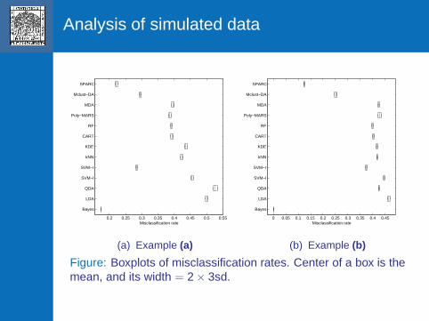
Analysis of simulated data

0.2 0.25 0.3 0.35 0.4 0.45 0.5 0.55

Bayes

LDA

QDA

SVM−l

SVM−r

kNN

KDE

CART

RF

Poly−MARS

MDA

Mclust−DA

SPARC

Misclassification rate

(a) Example (a)

0 0.05 0.1 0.15 0.2 0.25 0.3 0.35 0.4 0.45

Bayes

LDA

QDA

SVM−l

SVM−r

kNN

KDE

CART

RF

Poly−MARS

MDA

Mclust−DA

SPARC

Misclassification rate

(b) Example (b)

Figure: Boxplots of misclassification rates. Center of a box is themean, and its width = 2 × 3sd.

Analysis of simulated data

0 0.1 0.2 0.3 0.4 0.5

Bayes

LDA

QDA

SVM−l

SVM−r

kNN

KDE

CART

RF

Poly−MARS

MDA

Mclust−DA

SPARC

Misclassification rate

(a) Example (c)

0 0.05 0.1 0.15 0.2 0.25 0.3 0.35 0.4 0.45

Bayes

LDA

QDA

SVM−l

SVM−r

kNN

KDE

CART

RF

Poly−MARS

MDA

Mclust−DA

SPARC

Misclassification rate

(b) Example (d)

Figure: Boxplots of misclassification rates. Center of a box is themean, and its width = 2 × 3sd.

Real data

Hemophilia data : Available in the R packagerrcov. There are two classes of carrier andnon-carrier women. The variables aremeasurements on AHF activity and AHF antigen.

Biomedical data : Available in the CMU dataarchive. There are two classes of carriers andnon-carriers of a rare genetic disease. Variablesare four measurements on blood samples ofindividuals.

Analysis of real benchmark data sets

0.14 0.16 0.18 0.2 0.22 0.24

LDA

QDA

SVM−l

SVM−r

kNN

KDE

CART

RF

Poly−MARS

MDA

Mclust−DA

SPARC

Misclassification rate

(a) Hemophilia data

0.12 0.14 0.16 0.18 0.2 0.22

LDA

QDA

SVM−l

SVM−r

kNN

KDE

CART

RF

Poly−MARS

MDA

Mclust−DA

SPARC

Misclassification rate

(b) Biomedical data

Figure: Boxplots of misclassification rates. Center of a box is themean, and its width = 2 × 3sd.

Real data (Contd.)

Diabetes data : Available in the UCI data archive.There are three classes that consist of normalindividuals, chemical diabetic and overt diabeticpatients. The five variables are measurementsrelated to weights of individuals and their insulinand glucose levels in blood.

Vehicle data : Available in the UCI data archive.There are four types of vehicles and eighteenmeasurements related to the shape of eachvehicle.

Analysis of real benchmark data sets (Contd.)

0.05 0.1 0.15 0.2 0.25

LDA

QDA

SVM−l

SVM−r

kNN

KDE

CART

RF

Poly−MARS

MDA

Mclust−DA

SPARC

Misclassification rate

(a) Diabetes data

0.15 0.2 0.25 0.3 0.35 0.4

LDA

QDA

SVM−l

SVM−r

kNN

KDE

CART

RF

Poly−MARS

MDA

Mclust−DA

SPARC

Misclassification rate

(b) Vehicle data

Figure: Boxplots of misclassification rates. Center of a box is themean, and its width = 2 × 3sd.

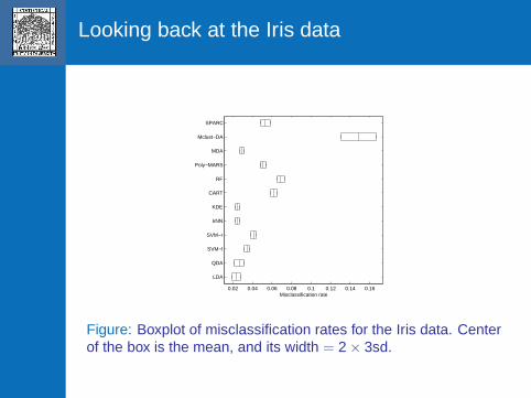
Looking back at the Iris data

0.02 0.04 0.06 0.08 0.1 0.12 0.14 0.16

LDA

QDA

SVM−l

SVM−r

kNN

KDE

CART

RF

Poly−MARS

MDA

Mclust−DA

SPARC

Misclassification rate

Figure: Boxplot of misclassification rates for the Iris data. Centerof the box is the mean, and its width = 2 × 3sd.