THE DVORETZKY–KIEFER–WOLFOWITZ INEQUALITY

WITH SHARP CONSTANT: MASSART’S 1990 PROOF

SEMINAR, SEPT. 28, 2011

R. M. Dudley

1

2

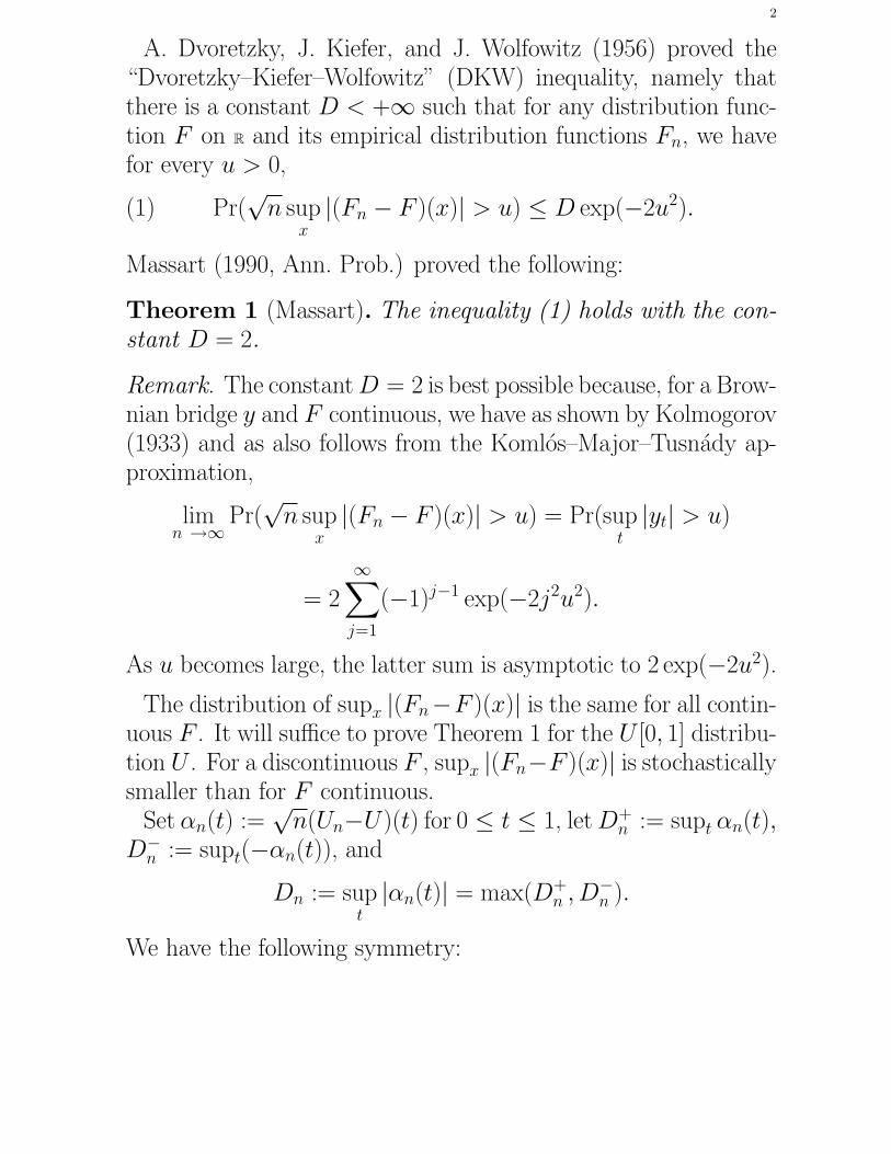
A. Dvoretzky, J. Kiefer, and J. Wolfowitz (1956) proved the“Dvoretzky–Kiefer–Wolfowitz” (DKW) inequality, namely thatthere is a constant D < +∞ such that for any distribution func-tion F on R and its empirical distribution functions Fn, we havefor every u > 0,

(1) Pr(√

n supx

|(Fn − F )(x)| > u) ≤ D exp(−2u2).

Massart (1990, Ann. Prob.) proved the following:

Theorem 1 (Massart). The inequality (1) holds with the con-stant D = 2.

Remark. The constant D = 2 is best possible because, for a Brow-nian bridge y and F continuous, we have as shown by Kolmogorov(1933) and as also follows from the Komlos–Major–Tusnady ap-proximation,

limn →∞

Pr(√

n supx

|(Fn − F )(x)| > u) = Pr(supt|yt| > u)

= 2

∞∑

j=1

(−1)j−1 exp(−2j2u2).

As u becomes large, the latter sum is asymptotic to 2 exp(−2u2).

The distribution of supx |(Fn−F )(x)| is the same for all contin-uous F . It will suffice to prove Theorem 1 for the U [0, 1] distribu-tion U . For a discontinuous F , supx |(Fn−F )(x)| is stochasticallysmaller than for F continuous.

Set αn(t) :=√

n(Un−U)(t) for 0 ≤ t ≤ 1, let D+n := supt αn(t),

D−n := supt(−αn(t)), and

Dn := supt|αn(t)| = max(D+

n , D−n ).

We have the following symmetry:

3

Proposition 2. For any n = 1, 2, ..., D+n and D−

n are equalin distribution.

Proof. (brief) Let X1, ..., Xn be the i.i.d. U [0, 1] variables onwhich Un is based. Let Yj := 1 − Xj for j = 1, ..., n. ThenY1, ..., Yn are i.i.d. U [0, 1] and for them, D−

n and D+n are inter-

changed for those of the Xj. ¤

Massart (1990, Theorem 1) gives the following fact, which isinteresting in itself and implies Theorem 1 (see the Remarks afterit):

Theorem 3. For any n = 1, 2, ... and any λ ≥ λn where λn =min(

√

log 2/2, ζn−1/6) and ζ := 1.0841, we have

(2) Pr(D−n > λ) ≤ exp(−2λ2).

Remarks. If exp(−2λ2) ≤ 1/2, then λ ≥√

(log 2)/2, whichimplies the hypothesis of Theorem 3. Also, Proposition 2 impliesPr(Dn > λ) ≤ 2 Pr(D−

n > λ). Further, Theorem 1 holds triviallyif 2 exp(−2λ2) > 1, so it suffices to prove Theorem 3 to proveTheorem 1 in all cases.

Proof. If for a given λ > 0,

(3) D−n =

√n sup

0≤t≤1(t − Un(t)) > λ,

then t−Un(t) = λ/√

n for some t, because between its downwardjumps at the observations Xj, t−Un(t) is continuously increasing.Let X(1) < X(2) < · · · < X(n) (almost surely) be the orderstatistics of X1, ..., Xn. Thus

sup0≤t≤1

t − Un(t) = max1≤k≤n

X(k) − (k − 1)/n

(the supremum occurs just to the left of some X(k)); the supremumis strictly positive with probability 1 because X(1) > 0. So if (3)

4

holds there is a smallest k = 1, ..., n with X(k) − (k − 1)/n >λ/

√n. Letting X(0) := 0, we must have t − Un(t) = λ/

√n for

some t with X(k−1) < t < X(k). Let τn := τn(λ) be the leastt ∈ [0, 1] such that t − Un(t) = λ/

√n if one exists (D−

n > λ),otherwise let τn = 2. If τn < 2, then for some j = 0, 1, ..., n − 1,τn − j/n = λ/

√n, i.e. τn = j

n + λ√n, which implies that

(4) j < n − λ√

n.

If λ ≥ √n then Pr(D−

n > λ) = 0, implying the conclusion of thetheorem, so suppose λ <

√n. Let J ≥ 0 be the largest integer

less than n − λ√

n.The following fact, according to Massart (1990), is due to Smir-

nov (1944).

Proposition 4 (Smirnov). For each λ with 0 < λ <√

n andε := λ/

√n, and each j = 1, ..., J , Pr(τn = ε + j/n) = pλ,n(j)

where

(5) pλ,n(j) = λ√

n(j + λ√

n)j−1(n − j − λ√

n)n−jn−n

(

n

j

)

.

For j = 0, Pr(τn = ε) = (1 − ε)n.

Proof. For each n, ε = λ/√

n and i = 1, ..., J let Ai :={

X(i) ≤ ε + i−1n

}

. Here is a

Claim. We have {τn = ε} = Ac1 and for j = 1, ..., J , {τn =

ε + jn} =

(

⋂

1≤i≤j Ai

)

∩ Acj+1.

Proof of Claim. This is straightforward and omitted.

Now continuing the proof of Proposition 4, X(1) has distributionfunction 1−(1−x1)

n and so density n(1−x1)n−1 for 0 ≤ x1 ≤ 1.

For 1 ≤ i < n, conditional on X(1), ..., X(i), X(i+1) is the least ofn − i variables i.i.d. U [X(i), 1] (this conditional distribution only

5

depends on X(i)). Thus Pr(X(i+1) ≥ t|X(i)) = ((1 − t)/(1 −X(i)))

n−i and the conditional density of X(i+1) given X(i) = xi is(n− i)(1− xi+1)

n−i−1/(1− xi)n−i. Iterating, the joint density of

X(1), ..., X(j+1) is n!(1 − xj+1)n−j−1/(n − j − 1)! for 0 ≤ x1 ≤

x2 ≤ · · · ≤ xj ≤ xj+1 ≤ 1 and 0 elsewhere. Thus

Pr

(

τn = ε +j

n

)

=n!

(n − j − 1)!IjJj

where

(6) Ij :=

∫ ε

0

dx1

∫ ε+1/n

x1

dx2 · · ·∫ ε+(j−1)/n

xj−1

dxj,

(7)

Jj :=

∫ 1

ε+(j/n)

(1− xj+1)n−j+1dxj+1 =

(

1 − ε − j

n

)n−j

/(n− j),

and a (j + 1)-fold integral equals the given product because xj ≤ε + (j − 1)/n and xj+1 ≥ ε + j/n imply xj ≤ xj+1. Also,(j/n) + ε < 1 follows from j ≤ J < n − λ

√n. So, to prove

Proposition 4 it remains to show that

(8) Ij = ε

(

j

n+ ε

)j−1

/j!.

This will be proved for each ζ with 0 < ζ ≤ 1 − j−1n in place of

ε and by induction on j. Equation (8) holds for j = 1. Assumeit holds for j − 1 for some j with 2 ≤ j ≤ J , and for each ζwith 0 ≤ ζ ≤ 1 − (j − 2)/n in place of ε. In the integral (6)make the changes of variables ξi = xi − x1 for i = 2, ..., j and letδ := ε − x1 + 1

n. Then

(9) Ij =

∫ ε

0

dx1

∫ δ

0

dξ2

∫ δ+1/n

ξ2

dξ3 · · ·∫ δ+(j−2)/n

ξj−1

dξj.

6

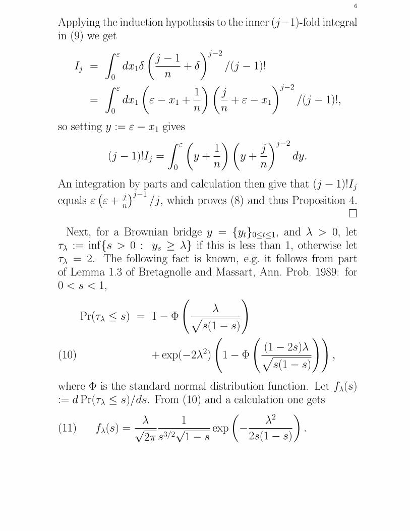
Applying the induction hypothesis to the inner (j−1)-fold integralin (9) we get

Ij =

∫ ε

0

dx1δ

(

j − 1

n+ δ

)j−2

/(j − 1)!

=

∫ ε

0

dx1

(

ε − x1 +1

n

) (

j

n+ ε − x1

)j−2

/(j − 1)!,

so setting y := ε − x1 gives

(j − 1)!Ij =

∫ ε

0

(

y +1

n

) (

y +j

n

)j−2

dy.

An integration by parts and calculation then give that (j − 1)!Ij

equals ε(

ε + jn

)j−1/j, which proves (8) and thus Proposition 4.

¤

Next, for a Brownian bridge y = {yt}0≤t≤1, and λ > 0, letτλ := inf{s > 0 : ys ≥ λ} if this is less than 1, otherwise letτλ = 2. The following fact is known, e.g. it follows from partof Lemma 1.3 of Bretagnolle and Massart, Ann. Prob. 1989: for0 < s < 1,

Pr(τλ ≤ s) = 1 − Φ

(

λ√

s(1 − s)

)

+ exp(−2λ2)

(

1 − Φ

(

(1 − 2s)λ√

s(1 − s)

))

,(10)

where Φ is the standard normal distribution function. Let fλ(s):= d Pr(τλ ≤ s)/ds. From (10) and a calculation one gets

fλ(s) =λ√2π

1

s3/2√

1 − sexp

(

− λ2

2s(1 − s)

)

.(11)

7

From the definitions we have for each λ > 0

(12) Pr(D−n > λ) =

∑

0≤j<n−λ√

n

pλ,n(j).

A well-known, simple reflection proof gives

(13) exp(−2λ2) = Pr(τλ ≤ 1) =

∫ 1

0

fλ(s)ds.

The next fact is one of the main steps in the proof of Theorem 3.

Proposition 5. Let j be a nonnegative integer with j <n − λ

√n. Let s = (2ε/3) + j/n , s′ = 1 − s, and vn(s) =

1/(

s(s2 − 1/(4n2))

. If nε ≥ 2, then

(14) pλ,n(j) ≤ 1

n

(

1 − ε

3s′+

ε2

6s′2

)

En,λ,s

where

(15) En,λ,s = exp

(

0.4

ns− ε2

24n(vn(s) + vn(s′))

)

fλ(s).

Some lemmas and other facts will be used to prove Proposition5. The first one has implications for the binomial distribution.

Lemma 6. Let 0 < ε < q = 1 − p < 1. Let

h(p, ε) = (p + ε) log

(

p + ε

p

)

+ (q − ε) log

(

q − ε

q

)

.

For t ≥ 0 let

g(t) = t − t2

2(1 + 2t/3)− log(1 + t).

Then(i) g is a strictly increasing convex function with g(t)/t → 1/4as t → +∞,

8

(ii) For t := ε/(q − ε),

h(p, ε) ≥ ε2

2(p + ε/3)(q − ε/3)+ εg(t)/t.

Proof. For (i), we have g(0) = 0, and for all t > 0

g′(t) = (t3/9)(1 + 2t/3)−2(1 + t)−1 > 0.

To see that g′ is increasing, note that (3+2t)2(1+t)/t3 is decreas-ing. So g is convex. As t → +∞, g(t)/t → 1 − 1/(4/3) = 1/4as stated.

For (ii), the proof by straightforward calculation is omitted. ¤

A consequence for the binomial distribution is:

Theorem 7. Let Sn be a binomial (n, p) random variable andsuppose that 0 < ε < q = 1 − p. Then

Pr(Sn − np ≥ nε) ≤ exp

(

− nε2

2(p + ε/3)(q − ε/3)

)

.

Proof. The probability is less or equal to{

(

p

p + ε

)p+ε (

q

q − ε

)q−ε}n

= exp(−nh(p, ε))

by Chernoff’s inequality (1952, Ann. Math. Statist.; Massart alsomentions Cramer’s name here). Then we can apply Lemma 6(ii).

¤

Now, let’s begin the proof of Proposition 5 for j ≥ 1. ByStirling’s formula with error bounds (Feller, vol. I), for 1 ≤ j < n,

(

n

j

)

≤ 1√2π

√

n

j(n − jnnj−j(n − j)−(n−j)Cj

where Cj := exp(−1/(12j + 1)). One plugs that bound into (5).Recalling h(·, ·) as in Lemma 6 and that s = 2ε/3 + j/n and

9

s′ = 1 − s, it follows that

pλ,n(j) ≤ λ

n√

2π

(

s − 2ε

3

)−1/2(

s +ε

3

)−1(

s′ +2ε

3

)−1/2

·

· exp(

−nh(

s′ − ε

3, ε

))

Cj.

Define ψ(t) for 0 ≤ t < ∞ by

(16) ψ(t) = − log(1 + t) +3

2log

(

1 +2t

3

)

.

Setting t = ε/(s− 2ε/3), which agrees with the definition of t inLemma 6(ii)), that Lemma gives(17)

pλ,n(j) ≤ Cj

n

(

1 +2ε

3s′

)−1/2

exp

(

−nεg(t)

t+ ψ(t)

)

fλ(s).

To bound the exponentiated term, we have the following.

Lemma 8. Let θ := 0.4833. Let g and ψ be the functionsdefined in Lemma 6 and (16) respectively. For t > 0 andν > 0 let

T (ν, t) := ν2g(t) − νtψ(t) +θt2

1 + 2t/3.

Then T (ν, t) > 0 for 0 < t ≤ ν.

Proof. (a) First suppose ν = t > 0. Then, straightforwardly wehave

(18)d

dt

(

T (t, t)

t2

)

=−2θ/3 − t/3 + t2/9

(1 + 2t/3)2.

The quadratic in the numerator has two roots, one being negative,and a positive root t0 = (3+

√9 + 24θ)/2. The derivative in (18)

equals −2θ/3 < 0 when t = 0, so t0 is a relative minimum

10

of T (t, t)/t2 and is the absolute minimum for t > 0. We findT (t0, t0)/t

20

.= 5.05 · 10−6 > 5 · 10−6 > 0, so T (t, t) > 0 for all

t > 0.(b) Now for general 0 < t ≤ ν, T is a quadratic polynomial in νfor fixed t. Its derivative with respect to ν is 2νg(t) − tψ(t). If

(19) 2g(t) − ψ(t) > 0

then T (ν, t) is increasing in ν for all ν > t and so T (ν, t) > 0.Or, if the discriminant D(t) of the quadratic polynomial satisfies

D(t) = t2ψ2(t) − 4g(t)θt2/(1 + 2t/3) < 0

or equivalently

(20) ∆(t) := (1 + 2t/3)ψ2(t) − 4θg(t) < 0

then T (t, ν) remains positive for all ν ≥ t as it is for ν = t andhas no roots. So to prove Lemma 8 it will suffice to show that(i) 2g(t) − ψ(t) > 0 for all t ≥ 3.37.(ii) ∆(t) < 0 for 0 < t ≤ 3.37.

Proof of (i). We have

2g′(t) − ψ′(t) =t

9(2t2 − 2t − 3)(1 + t)−1

(

1 +2t

3

)−2

.

We have 2t2 − 2t − 3 > 0 for t > (1 +√

7)/2, thus 2g − ψ isincreasing for such t. Since (1 +

√7)/2

.= 1.823 < 3.37 we have

that for t ≥ 3.37,

2g(t) − ψ(t) ≥ 2g(3.37) − ψ(3.37).= .000775 > 7 · 10−4 > 0,

proving (i).For (ii), Massart states that R(t) =

(

1 + 2t3

)

ψ2(t)/g(t) is in-creasing for t > 0 (which is only needed for t ≤ 3.37). The proofgiven in the first half of p. 1275 of his paper is not correct, asthe function R0 = ψ2/g is not increasing. Nevertheless it appears

11

true that R(t) is increasing by examining computed values of it ona grid, 0, 0.01, 0.02, ..., 3.37. (In a recent email, Massart said hehad independently verified the increasing property with a Matlabplot, but as of today, neither of us seems to have a rigorous proof.)It follows that (ii) holds.

To continue the proof of Proposition 5, three Claims will beused.

Claim 1. Let β := 0.826. Then for any x ∈ [0, 1],

(1 + 2x)−1/2 ≤(

1 − x +3x2

2

)

exp(−βx3).

This is proved by a straightforward calculation, omitted.

Claim 2. For ε = λ/√

n as usual and j, s, s′, and vn(·) asdefined in Proposition 5, if nε ≥ 2 and ns′ ≥ 1, we have

(21)

(

1 +2ε

3s′

)−1/2

≤(

1 − ε

3s′+

ε2

6s′2

)

exp

(

−ε2vn(s′)

24n

)

.

Proof of Claim 2. One can first check easily that ε ≤ 3s′. Thenwe can apply Claim 1 with x = ε/(3s′). The rest of the proof isa straightforward calculation, using the hypotheses. ¤

Claim 3. For vn as defined in Proposition 5, and any ε > 0 ands > 0 satisfying 1/n ≤ ε ≤ 3s/2, we have

(22)

(

1 + 12n

(

s − 2ε

3

))−1

≥ 1

12ns+

ε2vn(s)

24n.

Proof of Claim 3. This is another routine calculation. ¤

12

Now to finish the proof of Proposition 5 for j ≥ 1, recall (17).Note that t = nε/j ≤ nε. Lemma 8 with ν = nε gives

pλ,n(j) ≤ Cj

n

(

1 +2ε

3s′

)−1/2

exp

(

θ

ns

)

fλ(s).

Claim 2 gives an upper bound for(

1 + 2ε3s′

)−1/2and Claim 3 gives

one for Cj. Noting that θ − 1/12 < 0.4 finishes the proof forj ≥ 1.

Proof of Proposition 5 for j = 0. In this case s = 2ε/3. Wehave pλ,n(0) = (1 − ε)n by Proposition 4. It’s natural to defineh(p, δ) when δ = q as − log(p) since for fixed q with 0 < q < 1,(q − δ) log((q − δ)/q) → 0 as δ ↑ q, so that will be done. Then(1 − ε)n = exp(−nh(1 − ε, ε)). To apply Lemma 6, we will havet = ε/(q− ε) which it’s natural to define as +∞ in this case withq = ε; for t → +∞ the limit of g(t)/t is 1/4. Then Lemma 1gives

pλ,n(0) = (1 − ε)n = exp(−nh(1 − ε, ε) ≤ exp

(

− λ2

2ss′− nε

4

)

.

Define H(ν) for ν > 0 by

H(ν) :=3 log(3/2)

2− log(2π)

2+

ν

4+

0.4

ν− log(ν)

2.

Then it’s straightforward to check that

(1 − ε)n ≤ λ√2πn

s−3/2 exp

(

0.4

nε

)

exp

(

− λ2

2ss′

)

exp(−H(nε).

We have H ′(ν) = 14 − 0.4

ν2 − 12ν = 0 if and only if ν2−2ν−1.6 = 0.

The only positive root of this is at ν0 = 1 +√

2.6. This is theminimum of H for ν > 0 because H(ν) → +∞ as ν → +∞.

13

Thus H(ν) ≥ H(ν0) ≥ 0.01534 > 0 for all ν > 0. It follows that

pλ,n(0) ≤ λ√2πn

s−3/2 exp

(

0.4

nε

)

exp

(

− λ2

2ss′

)

≤ 1

n

(

1 +2ε

3s′

)−1/2

exp

(

0.4

nε

)

fλ(s),

where the second equation follows on expanding fλ(s) by (11).Since nε ≥ 2, it follows that

ε2vn(s)

24n≤

(

16nε

(

4

9− 1

16

))−1

≤ 9/(55nε),

from which it follows that

0.4

nε+

ε2vn(s)

24n≤ 0.4 + 9/55

nε≤ 0.4

ns.

Combining gives

Pλ,n(0) ≤ 1

n

(

1 +2ε

s′

)−1/2

exp

(

0.4

ns− ε2vn(s)

24n

)

fλ(s).

Via Claim 2, (14) follows and Proposition 5 is proved. ¤

In the proof of Theorem 3, the integral in (13) will be com-pared to Riemann sums and thereby to the sums in (12). Thecomparison will use the next lemma.

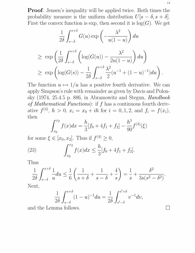
Lemma 9. Let 0 < δ ≤ s ≤ 1 − δ and s′ = 1 − s. If G is acontinuous function with G(x) > 0 for s − δ ≤ x ≤ s + δ andlog(G) is convex, then for any λ > 0,

1

2δ

∫ s+δ

s−δ

G(u) exp

(

− λ2

2u(1 − u)

)

du ≥ G(s) · exp

(

− λ2

2ss′

)

·

· exp

(

−λ2δ2

6

(

(

s(s2 − δ2))−1 (

s′(s′2 − δ2))−1

)

)

.

14

Proof. Jensen’s inequality will be applied twice. Both times theprobability measure is the uniform distribution U [s − δ, s + δ].First the convex function is exp, then second it is log(G). We get

1

2δ

∫ s+δ

s−δ

G(u) exp

(

− λ2

u(1 − u)

)

du

≥ exp

(

1

2δ

∫ s+δ

s−δ

(

log(G(u)) − λ2

2u(1 − u)

)

du

)

≥ exp

(

log(G(s)) − 1

2δ

∫ s+δ

s−δ

λ2

2(u−1 + (1 − u)−1)du

)

.

The function u 7→ 1/u has a positive fourth derivative. We canapply Simpson’s rule with remainder as given by Davis and Polon-sky (1974, 25.4.5 p. 886, in Abramowitz and Stegun, Handbookof Mathematical Functions): if f has a continuous fourth deriv-ative f (4), h > 0, xi = x0 + ih for i = 0, 1, 2, and fi = f(xi),then

∫ x2

x0

f(x)dx =h

3[f0 + 4f1 + f2] −

h5

90f (4)(ξ)

for some ξ ∈ [x0, x2]. Thus if f (4) ≥ 0,

(23)

∫ x2

x0

f(x)dx ≤ h

3[f0 + 4f1 + f2].

Thus

1

2δ

∫ s+δ

s−δ

1

udu ≤ 1

6

(

1

s + δ+

1

s − δ+

4

s

)

=1

s+

δ2

3s(s2 − δ2).

Next,

1

2δ

∫ s+δ

s−δ

(1 − u)−1du =1

2δ

∫ s′+δ

s′−δ

v−1dv,

and the Lemma follows. ¤

15

Next are some identities for special integrals.

Lemma 10. For any a ≥ 0, b ≥ 0, and λ > 0, let Ia,b(λ) =

λ exp(2λ2)√2π

∫ 1

0

u−a−1/2(1 − u)−b−1/2 exp

(

− λ2

2u(1 − u)

)

du.

Then the following hold:(i) I1,1(λ)/2 = I1,0(λ) = 1;(ii) I2,2(λ) = I2,1(λ) = 4 + λ−2;(iii) I2,0(λ) = 2 + λ−2.

Proof. Clearly Ia,b ≡ Ib,a. For any u with 0 < u < 1,

u−1/2−a(1−u)−1/2−b−(1−u)−1/2−bu1/2−a = u−1/2−a(1−u)1/2−b,

which implies for any a ≥ 1 and b ≥ 1 that

(24) Ia,b = Ia−1,b + Ia,b−1.

For a = b = 1, using exp(−2λ2) =∫ 1

0 fλ(s)ds (13) where

fλ(s) =λ√2π

1

s3/2√

1 − sexp

(

− λ2

2s(1 − s)

)

(11), we get (i). Next, differentiating with respect to λ gives (ii).Then, applying (24) with a = 1 and b = 2, (iii) follows from (i)and (ii). So Lemma 10 is proved. ¤

Now we can prove Theorem 3 under some conditions.

Proof of Theorem 3 for n ≥ 39 and λ ≤ √n/2. Since n ≥ 39,

the hypothesis on λ in Theorem 3 becomes λ ≥ ζn−1/6. Thusnε = λ

√n ≥ 3.6764. Define the function y(·) by y(x) := (ex −

1)/x for x > 0. It’s easily seen (e.g. from the Taylor series) thatthis function is increasing. Recalling that s ≥ 2ε/3 we have

exp

(

0.4

ns

)

≤ 1 + y

(

0.6

3.6764

)

0.4

ns.

16

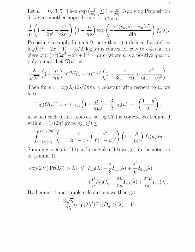
Let µ := 0.4345. Then exp(

0.4ns

)

≤ 1 + µns. Applying Proposition

5, we get another upper bound for pλ,n(j):

1

n

(

1 − ε

3s′+

ε2

6s′2

)

(

1 +µ

ns

)

exp

(

−ε2(vn(s) + vn(s′)

24n

)

fλ(s).

Preparing to apply Lemma 9, note that z(·) defined by z(x) =log(6x2 − 2x + 1) − (5/2) log(x) is convex for x > 0: calculationgives z′′(x)x2(6x2− 2x+ 1)2 = h(x) where h is a positive quarticpolynomial. Let G(u) :=

λ√2π

(

1 +µ

nu

)

u−3/2(1 − u)−1/2

(

1 − ε

3(1 − u)+

ε2

6(1 − u)2

)

.

Then for c := log(λ/(6√

2πε), a constant with respect to u, wehave

log(G(u)) = c + log(

1 +µ

nu

)

− 3

2log(u) + z

(

1 − u

ε

)

,

in which each term is convex, so log G(·) is convex. So Lemma 9with δ = 1/(2n) gives pλ,n(j) ≤

∫ s+1/(2n)

s−1/(2n)

(

1 − ε

3(1 − u)+

ε2

6(1 − u)2

)

(

1 +µ

nu

)

fλ(u)du.

Summing over j in (12) and using also (13) we get, in the notationof Lemma 10,

exp(2λ2) Pr(D−n > λ) ≤ I1,0(λ) − ε

3I1,1(λ) +

ε2

6I2,1(λ)

+µ

nI2,0(λ) − εµ

3nI2,1(λ) +

ε2µ

6nI2,2(λ).

By Lemma 4 and simple calculations we then get

3√

n

2λ(exp(2λ2) Pr(D−

n > λ) − 1)

17

≤ ηn(λ) := −1 +

(

λ +1

4λ+

3µ

λ+

3µ

2λ3

)

n−1/2

−µ

2

(

4 +1

λ2

)

n−1 +µ

2

(

4λ +1

λ

)

n−3/2.(25)

Remark. Smirnov (1944), as quoted by Massart, had given theasymptotic expansion

(26) Pr(D−n > λ) ∼ exp(−2λ2)

(

1 − 2λ

3√

n+ O(1/n)

)

if λ = O(n1/6). By contrast, Massart’s inequality (25) is one-sided, but the first term −1 on the right confirms that the term−2λ/(3

√n) in Smirnov’s expansion is valid non-asymptotically

in a one-sided sense, which is what one wants.

It is easy to check that ηn is convex in λ for each n. Thus, toshow that ηn(λ) < 0 for ζn−1/6 ≤ λ ≤ √

n/2 it will suffice toshow that an := ηn(ζn−1/6) < 0 and bn := ηn(

√n/2) < 0.

It will be shown that an and bn are decreasing in n for n ≥ 39.We have

an = ηn(ζn−1/6) = −1 +(

ζn−1/6

+n1/6

ζ

(

1

4+ 3µ

)

+3µ

2

n1/2

ζ3

)

n−1/2

−µ

2

(

4 +n1/3

ζ2

)

n−1 +µ

2

(

4ζn−1/6 +n1/6

ζ

)

n−3/2

= −1 +3µ

2ζ3+ n−1/3

(

1

ζ

) (

1

4+ 3µ

)

+

(

ζ − µ

2ζ2

)

n−2/3

−2µn−1 +µ

2ζn−4/3 + 2µζn−5/3.

18

As ζ = 1.0841 (Theorem 3) and µ = 0.4345, ζ − µ/(2ζ)2 >0. Terms with positive coefficients and negative powers of n, orwith negative coefficients and positive powers of n, are decreasing.Just one term, −2µn−1, is increasing. It will suffice to showthat (3/ζ)n−1/3 − 2n−1 is decreasing for n ≥ 39, or that 3x −2.1682x3 is increasing for 0 < x ≤ 1/39. Indeed its derivative ispositive there. A calculation shows that bn is a linear combinationof negative powers of n times positive coefficients, so it is alsodecreasing in n. We have a39

.= −0.006382 < 0 and b39

.=

−0.4238 < 0, so both an and bn are negative for all n ≥ 39, andηn(λ) < 0 for ζn−1/6 ≤ λ ≤ √

n/2. So Theorem 3 is proved forn ≥ 39 and λ ≤ √

n/2.

Let Cλ,n = exp(2λ2) Pr(D−n > λ).

Proposition 11. Let n ≥ 2 and let λ be such that 0 < λ <√n. Then

(i) For λ ≥ √n/2, d

dλCλ,n ≤ 0,

(ii)∑n−1

j=1 jj−1(n − j)n−jn−n(

nj

)

≤ 1,

(iii) For λ ≥ 1/2, we have ddλCλ,n ≤ 3.61.

Proof. (i) Let Lλ,n(j) = log(exp(2λ2)pλ,n(j) for 0 ≤ j < n −λ√

n. Since

Pr(D−n > λ) =

∑

0≤j<n−λ√

n

pλ,n(j).

by (12), it will suffice to show that for each such j, dLλ,n/dλ < 0for λ ≥ √

n/2. The proof of this is by calculations, where thecase j = 0 is relatively easy but separate, and the case j ≥ 1takes more but not especially long calculation. So (i) holds.

19

(ii) By (12) and (5) we have

d

dλPr(D−

n > λ)∣

∣

∣

λ=0=√

n

n−1∑

j=1

jj−1(n − j)n−jn−n

(

n

j

)

− 1

.

By part (i), Pr(D−n > λ) is nonincreasing with respect to λ, so

(ii) follows.(iii) First suppose nε ≥ 2 and ε ≤ 1/2. Using Proposition 5

and the bound exp(0.4/(ns)) ≤ exp(0.3), in the same way as inthe proof of Theorem 3 for n ≥ 39 and ε ≤ 1/2, we now get

Cλ,n ≤ e0.3

(

I1,0(λ) − ε

3I1,1(λ) +

ε2

6I2,1(λ)

)

.

Using Lemma 10 and 2/√

n ≤ λ ≤ √n/2, it follows that

Cλ,n ≤ e0.3 +2λ

3√

ne0.3

(

−1 +

(

λ +1

4λ

)

n−1/2

)

≤ e0.3 +2λ

3√

ne0.3

(

−3

8

)

.

Combining with (i) gives

(27) Cλ,n ≤ exp(max((8/n), 0.3))

for any integer n ≥ 4 and any λ > 0.By Lemma 6 one gets an alternate bound, useful for smaller

values of n,

pλ,n(j) ≤ λ√

n

(

n

j

)

jj−1(n − j)n−jn−n exp(−2λ2).

Thus by (ii),

(28) Cλ,n ≤ λ√

n + pλ,n(0) exp(2λ2).

20

For j = 0,, dLλ,n(0)/dλ < 0, and for 1 ≤ j < n − λ√

n,dLλ,n(j)/dλ < 1/λ. Thus

d

dλCλ,n ≤ 1

λ

(

Cλ,n − pλ,n(0) exp(2λ2))

.

Combining this last inequality with (27) if n ≥ 14, or (28) forn ≤ 13, we get

d

dλCλ,n ≤ max(2 exp(4/7),

√13) ≤ 3.61,

which proves (iii) and so Proposition 11. ¤

Proof of Theorem 3 for n ≤ 38 or λ >√

n/2. By Proposition11 and the first part of the proof of Theorem 3, we can assumethat n ≤ 38. Then the assumption on λ in Theorem 3 reduces toλ ≥

√

(log 2)/2 which implies λ > 1/2.Letting η := 0.01, let Λη,m = {1

2 + kη : k ∈ N} ∩[

12,√

n)

. Acomputer calculation, reported by Massart (1990), gave

(29) maxn≤38

maxλ∈Λη,n

Cλ,n ≤ 0.951.

In a confirming computation, the maximum was found to be.=

0.94955, attained at n = 38 and λ = 1/2. Combining (29) withProposition 11(iii), we get

maxn≤38

sup1/2≤λ<

√n

Cλ,n ≤ 0.951 + 3.61η ≤ 0.9871 < 1,

which finishes the proof of Theorem 3 for n ≤ 38 and so completesits proof. ¤

Komlos, Major, and Tusnady (1975, ZW) stated a sharp rateof convergence in Donsker’s theorem, namely that on some prob-ability space there exist Xi i.i.d. U [0, 1] and Brownian bridges Yn

21

such that

P

(

sup0≤t≤1

|(αn − Yn)(t)| >x + c log n√

n

)

< Ke−λx(30)

for all n = 1, 2, . . . and x > 0, where c, K, and λ are positiveabsolute constants.

More specifically, Bretagnolle and Massart (1989, Ann. Prob.)proved the following:

Theorem 12 (Bretagnolle and Massart). The approximation(30) of empirical processes by Brownian bridges holds withc = 12, K = 2 and λ = 1/6 for n ≥ 2.

The Dvoretzky–Kiefer–Wolfowitz–Massart inequality, Theorem1, gives us some crude bounds so that we can see how large n needsto be for Theorem 12 to be effective. Namely, for any empiricalprocess αn, any Brownian bridge Y , and any b > 0, we have

Pr(supt|(αn − Y )(t)| ≥ b) ≤

Pr(supt|αn(t)| ≥ b/2) + Pr(sup

t|Y (t)| ≥ b/2) ≤ 4 exp(−b2/2),

not depending on n. If b ≥ 2.97 then 4 exp(−b2/2) ≤ 0.05, so αn

and Yn will very likely be within b of each other in sup norm justbecause both will probably be bounded in absolute value by b/2.If we choose x = 3 log n in (30) then with λ = 1/6 the bounds forprobabilities on the right in (30) will decrease just at a moderateO(1/

√n) rate. Then we would like 15(log n)/

√n < 2.97 to get

a bound better than the crude one, in other words (log n)/√

n ≤0.198. This does not hold for n = 1000, or 1300, but it does holdfor n = 1320.

Bretagnolle and Massart’s theorem is proved in more detail thanthey gave in my notes for a summer course on empirical processesin 1999 (MaPhySto, Denmark). I plan to include the proof, as

22

well as that of Massart’s (1990) theorem, in the second edition ofmy book Uniform Central Limit Theorems.

Z. W. Birnbaum and F. H. Tingey, Ann. Math. Statist. 22

(1951), pp. 592-596, in Sections 2 and 3, give a brief but perhapssufficient proof of Proposition 4. They cite two references, oneof which is by Smirnov, but from 1939, not 1944. The 1944 pa-per seems relatively hard to access. I found the Birnbaum andTingey reference from the natural source, namely the book by G.R. Shorack and G. Wellner, Empirical Processes with Applica-tions to Statistics, originally published by Wiley in 1986, reissuedin the Classics in Applied Mathematics series of the Society forIndustrial and Applied Mathematics, 2009.