The Cryosphere, 11, 1519–1535, 2017https://doi.org/10.5194/tc-11-1519-2017© Author(s) 2017. This work is distributed underthe Creative Commons Attribution 3.0 License.

SEMIC: an efficient surface energy and mass balancemodel applied to the Greenland ice sheetMario Krapp1,2, Alexander Robinson3,1, and Andrey Ganopolski11Potsdam Institute for Climate Impact Research (PIK), P.O. Box 60 12 03, 14412 Potsdam, Germany2Department of Zoology, University of Cambridge, Cambridge CB2 3EJ, UK3Departamento de Astrofísica y Ciencias de la Atmósfera, Universidad Complutense de Madrid, 28040 Madrid, Spain

Correspondence to: Mario Krapp (mariokrapp@gmail.com)

Received: 25 October 2016 – Discussion started: 14 November 2016Revised: 13 May 2017 – Accepted: 16 May 2017 – Published: 3 July 2017

Abstract. We present SEMIC, a Surface Energy and Massbalance model of Intermediate Complexity for snow- andice-covered surfaces such as the Greenland ice sheet. SEMICis fast enough for glacial cycle applications, making it a suit-able replacement for simpler methods such as the positivedegree day (PDD) method often used in ice sheet modelling.Our model explicitly calculates the main processes involvedin the surface energy and mass balance, while maintaininga simple interface and requiring minimal data input to driveit. In this novel approach, we parameterise diurnal tempera-ture variations in order to more realistically capture the dailythaw–freeze cycles that characterise the ice sheet mass bal-ance. We show how to derive optimal model parameters forSEMIC specifically to reproduce surface characteristics andday-to-day variations similar to the regional climate modelMAR (Modèle Atmosphérique Régional, version 2) and itsincorporated multilayer snowpack model SISVAT (Soil IceSnow Vegetation Atmosphere Transfer). A validation testshows that SEMIC simulates future changes in surface tem-perature and surface mass balance in good agreement withthe more sophisticated multilayer snowpack model SISVATincluded in MAR. With this paper, we present a physicallybased surface model to the ice sheet modelling communitythat is general enough to be used with in situ observations,climate model, or reanalysis data, and that is at the same timecomputationally fast enough for long-term integrations, suchas glacial cycles or future climate change scenarios.

1 Introduction

Currently, surface melt accounts on average for about half ofthe observed Greenland ice sheet loss; the other half is lostthrough basal melt and ice discharge across the groundingline, i.e. calving (van den Broeke et al., 2009). Recent obser-vations show that Greenland’s surface mass balance is furtherdeclining (Hanna et al., 2013). The positive surface mass bal-ance can no longer compensate for losses via ice dischargeand is therefore regarded as a dominant source of Green-land’s total mass loss. The extreme melt season in 2012 ex-posed the Greenland ice sheet’s vulnerability to long-lastingtemperatures anomalies (Nghiem et al., 2012). As more ma-rine terminating glaciers further retreat (Thomas et al., 2011),the partitioning of ice loss is likely to shift further towards thedeclining surface mass balance.

Numerical simulations of large land ice masses, such asthe Greenland and the Antarctic ice sheets, require numericalmodels to be fast because the response time of ice sheets tochanges in the surface mass balance is slow, on the orderof years to tens of millennia (Cuffey and Paterson, 2010).Hence, many thousands of years of model integrations arerequired to spin up the model or to simulate one or severalglacial cycles.

The simplest, fastest, and still most widely used method toestimate the surface mass balance of glaciers and ice sheetsis the so-called positive degree day (PDD) approach (e.g.Reeh, 1991; Ohmura, 2001). It is based on the empirical re-lationship between surface melt rate and daily mean surfaceair temperature. Although PDD parameters are tuned to cor-rectly represent present-day melting rates, past climates may

Published by Copernicus Publications on behalf of the European Geosciences Union.

1520 M. Krapp et al.: SEMIC: an efficient surface energy and mass balance model

require different parameter values. For instance, the PDD ap-proach with its present-day parameter values is not applica-ble to orbitally forced climate change (van de Berg et al.,2011; Robinson and Goelzer, 2014).

The importance of climatic changes in the past to the sen-sitivity of the Greenland ice sheet has already been acknowl-edged in one of the first attempts to utilise an energy-balancemodel for a sensitivity study (Oerlemans, 1991). Under awarming climate an energy-balance approach is superior tothe relatively simple PDD method and “snowpack proper-ties evolve on a multidecadal timescale to changing climate,with a potentially large impact on the mass balance of the icesheet” (Bougamont et al., 2007).

Here, we propose a physically based model utilising anenergy-balance approach that is inherently consistent witha variety of climate states different from today, e.g. fu-ture warming, last glacial maximum, or the Eemian inter-glacial. Our proposed model not only accounts for temper-ature changes but also for changes in other climate factors,such as insolation, turbulent heat fluxes, and surface albedo.

The Surface Energy and Mass balance model of Interme-diate Complexity (SEMIC) is based on a surface schemethat has already been used to study glacial cycles (Calovet al., 2005). SEMIC provides a process-based relationshipbetween surface energy and surface mass balance changes.The approach described here guarantees a consistent treat-ment of melting and melt water refreezing; both are impor-tant processes for the mass budget of ice sheets (Reijmeret al., 2012).

Compared to more sophisticated multilayer snowpackmodels, which include snow metamorphism or vertical tem-perature profile calculations (e.g. Vionnet et al., 2012),SEMIC has a reduced complexity, one-layer snowpack. Thissaves computation time and allows for integrations on multi-millennial timescales. SEMIC calculates the daily surface en-ergy and mass balance throughout the year but is also fastenough to focus on longer timescales when climatologicalchanges determine the trend of the surface energy and massbalance.

Numerical ice sheet models need the annual mean surfacetemperatures and annual mean surface mass balance of iceas boundary conditions at the surface. Both are calculatedby SEMIC, which can thus be directly coupled to the icesheet model. There is a multitude of possible applicationsfor SEMIC, for example, under projections of future warm-ing for the next centuries or glacial cycle simulations. In thispaper, we will discuss the future warming projections of theRCP8.5 scenario (Moss et al., 2010) to demonstrate the ca-pabilities of our model.

The paper is organised as follows. In the next section, wepresent the model equations and their parameters. In Sect. 3,we describe the calibration procedure used to constrain thefree model parameters and we estimate the sensitivity of thecalculated surface mass balance with respect to the modelparameters. In Sect. 4, we validate our model against regional

climate model data for a future warming scenario. We discussour findings in Sect. 5 and conclude in Sect. 6.

With this paper we acknowledge, support, and encour-age research that follows standards with respect to scientificreproducibility, transparency, and data availability (Krapp,2017a). The model source code and the authors’ manuscriptsource is freely available and accessible online.

2 Model description

SEMIC is based on the calculation of the mass and energybalance of the snow and/or ice surface (see, for example,Greuell et al., 2004). We assume that the surface tempera-ture Ts responds to changes in the surface energy balanceaccording to

ceffdTs

dt= (1−α)SW↓+LW↓−LW↑−HS−HL−QM/R, (1)

where α is the surface albedo, SW↓ is the downwelling short-wave radiation, (1−α)SW↓ is the net shortwave radiationSWnet. LW↓ is the downwelling longwave radiation, LW↑ isthe upwelling longwave radiation, HS and HL are the sen-sible and latent heat flux to the atmosphere, and QM/R isthe energy flux related to phase transitions, i.e. for melting orrefreezing of snow and ice. The parameter ceff denotes the ef-fective heat capacity of the snowpack. In a strict sense of theterm “energy balance” the left-hand side of Eq. (1) should bezero. Here, we assume that surface temperature and the en-ergy are not in equilibrium because the snowpack or surfaceexerts some thermal inertia.

Temperatures of snow- and ice-covered surfaces cannotexceed 0 ◦C. However, for computational purposes, we ini-tially assume that Ts represents the potential temperaturewhich would be observed in the absence of phase transitions,i.e. melting or refreezing. Once melting and refreezing hasbeen computed (see Sect. 2.3), the residual heat flux QM/R

in Eq. (1) keeps track of any heat flux surplus or deficit and isadded back to the energy balance. This way, Ts never exceeds0 ◦C over snow and ice.

For coupling to an ice sheet model, the surface mass bal-ance for ice (SMBi) is computed by SEMIC. It separates thetotal surface mass balance into the surface mass balance forsnow and for ice:

SMB= SMBs+SMBi = Ps− SU −M +R, (2)SMBs = Ps− SU −Msnow−Csi, (3)SMBi = Csi −Mice+R. (4)

Here, Ps is the snowfall rate and SU is the sublimation rate,which is related to the latent heat flux via HL/ρwLs, with ρwand Ls being water density and latent heat of sublimation,respectively (see Table 1). The model variable M is the totalmelting rate, i.e. the sum of snow and ice melt (denoted bythe subscripts), R is the refreezing rate of liquid water (rain

The Cryosphere, 11, 1519–1535, 2017 www.the-cryosphere.net/11/1519/2017/

M. Krapp et al.: SEMIC: an efficient surface energy and mass balance model 1521

Table 1. Model constants and their description.

Symbol Value Description

1t 86400s time step of 1 dayceff 2 · 106 Jm−3 effective heat capacity snow/ice (volumetric)CS 2.0 · 10−3 sensible heat exchange coefficientCL 0.5 · 10−3 latent heat exchange coefficientcp,a 1,000Jkg−1K−1 specific heat capacity of airσ 5.67 · 10−8 Wm−2K−4 Stefan–Boltzmann constantT0 273.15K freezing point of waterρw 1,000kgm−3 density of liquid waterLs 2.83 · 106 Jkg−1 latent heat of sublimationLv 2.5 · 106 Jkg−1 latent heat of vaporisationLm 3.3 · 105 Jkg−1 latent heat of melting (Ls−Lv)hs,max 5.0m maximum snow height (cut-off)

or melt water), and Csi is the compaction rate of snow whichis turned into ice.

Changes in snowpack height hs (in metre water equivalent)are determined by the surface mass balance of snow:

dhs

dt= SMBs, with hs ∈max(0,hs,max). (5)

If the snow height hs exceeds a certain threshold hs,max (hereset to 5 m), snow is transformed into ice – in a simple wayresembling snow compaction:

1t∫0

Csi dt =max(0,hs−hs,max). (6)

The described equations are solved using an explicit time-step scheme with a time step of 1 day. In principle, the useof monthly input data is also supported but would requireinterpolation to daily time steps.

2.1 Surface heat fluxes

We describe the outgoing longwave radiation as a function ofsurface temperature according to the Stefan–Boltzmann law:

LW↑ = σT 4s . (7)

For the turbulent heat exchange (sensible and latent) we usea standard bulk formulation (e.g. Gill, 1982):

HS = CSρacp,aus(Ts− Ta), (8a)HL = CLρaLsus(qs− qa), (8b)

with sensible and latent heat exchange coefficients CS andCL, air density ρa, specific heat capacity of air cp,a, surfacewind speed us, air temperature Ta, latent heat of sublima-tion/deposition Ls, and air specific humidity qa. Air den-sity ρa is not available from MAR and is thus approximatedby the ideal gas law ρa =

pRsTa

, with specific gas constant

Rs = 258Jkg−1K−1 and surface pressure p, which is avail-able from MAR. Specific humidity over the snow or ice sur-face (qs) is assumed to be saturated and depends on surfacepressure ps and saturation water vapour pressure e∗:

qs =e∗ε

e∗(ε− 1)+ps, where

e∗ = 611.2exp(a

Ts− T0

Tb+ Ts− T0

), (9)

with ε = 0.62197, the ratio of the molar weights of wa-ter vapour and dry air, and coefficients a and Tb, whichare prescribed for vapour pressure over water (a = 17.62,Tb = 243.12 K) or ice/snow (a = 22.46, Tb = 272.62 K). T0denotes the freezing point of water, 273.15 K. See Gill (1982)for more details.

2.2 The diurnal cycle of thawing and freezing

Because we use daily time steps, processes on timescalesshorter than 1 day cannot be resolved explicitly. Hence, wecannot explicitly account for the thawing during daytime andthe freezing during nighttime which is quite usual for themelting season on Greenland. The absorbed shortwave ra-diation, for example, can exhibit large diurnal variations, es-pecially when the surface albedo is low (Cuffey and Pater-son, 2010). During the day, near-surface temperatures mayrise above freezing temperature and snow or ice may start tomelt. During the night, temperatures drop below freezing andany liquid water such as previously melted water can refreezewithin the snowpack.

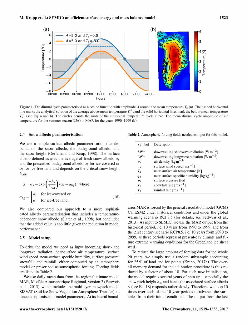
To account for this process we introduce a parameterisa-tion for the diurnal cycle of thawing and freezing. We simplyassume a sinusoidal temperature curve T (t) throughout theday (here, units of time t are hours h) around a given meansurface temperature Ts (here, we refer to Ts with units in ◦C)with amplitude A, i.e. a cosine function (Fig. 1a):

T (t)= Ts−Acos(2π24t). (10)

www.the-cryosphere.net/11/1519/2017/ The Cryosphere, 11, 1519–1535, 2017

1522 M. Krapp et al.: SEMIC: an efficient surface energy and mass balance model

For the sake of simplicity we use a single constant A, al-though in reality it is spatially and temporally dependent asshown in Fig. 1b.

Melting and refreezing may then occur on the same day if(potential, not actual) Ts exceeds 0 ◦C. The amount of melt-ing and refreezing then depends on the amplitude A and themean daily temperature Ts (Fig. 1a). Fortunately, an analyt-ical solution to this problem exists. We calculate the rootsof the cosine function and then integrate between the rootsto solve for average above- and below-freezing mean surfacetemperatures T +s and T −s . The roots are

t1 =242π

arccos(Ts

A) t2 = 24− t1.

Thus, the time span for temperatures above and below freez-ing is

1t+ = t2− t1 = 24− 2t1, and 1t− = 2t1.

This leads us to an expression for averages of above- andbelow-freezing temperatures T +s and T −s . These are the inte-grals of the cosine function:

T +s =11t+

t2∫t1

T (t)dt

=24

π1t+

−Ts arccos(Ts

A)+A

√1−

T 2s

A2 +πTs

,(11a)

T −s =11t−

t1∫0

T (t)dt +

24∫t2

T (t)dt

=

24π1t−

Ts arccos(Ts

A)−A

√1−

T 2s

A2

. (11b)

This parameterisation depends on the prescribed diurnalcycle amplitude, A, which affects the amount of melting andrefreezing and, thus, the surface mass balance. Note, meltenergyQm and “cold content”Qc in the following Eq. (12b)are calculated by using T +s and T −s , respectively. Withoutthis parameterisation or with A set to zero, melting and re-freezing cannot occur at the same time step, and, instead, theactual surface temperature Ts must be used.

2.3 Melting and refreezing

Additional processes that affect the snowpack temperatureare melting and refreezing. During the course of 1 day theenergy available for melt Qm and refreezing (the so-calledcold content) Qc are defined as

Qm =

{(T +s − T0)

ceff1t

if T +s > T0,

0 if T +s ≤ T0,(12a)

and

Qc =

{0 if T −s ≥ T0,

(T0− T−s )

ceff1t

if T −s < T0.(12b)

Thus, the potential melt is

Mpot =Qm

ρwLm, (13)

with latent heat of melting (or fusion) Lm and time step 1t .Actual melt depends on how much snow or ice is availablefor melt. If potential melt is larger than the current snowheight, all snow melts down and the excess melt energy isused to melt the underlying ice. Ice-free land is treated dif-ferently and the excess melt energy is used to warm the sur-face. The actual melt M is then the sum of melted snow andmelted ice:

Msnow =min(Mpot,hs/1t), (14a)Mice =Mpot−Msnow, (14b)M =Msnow+Mice. (14c)

The refreezing rate depends on the potential liquid waterto be refrozen, i.e. the actual melt rate M and rainfall Pr.Analogous to the melt rates, the potential refreezing is givenby

Rpot =Qc

ρwLm. (15)

Suppose some rain or melt water exists within the snow pack.The cold content Qc is then used to (virtually) turn this liq-uid water into frozen water, i.e. snow or ice. We distinguishbetween refrozen rain and refrozen melt water:

Rpot,rain =min(Rpot,Pr), (16a)Rpot,melt =min(max(Rpot−Rpot,rain,0),Msnow), (16b)

R = Rrain+Rmelt = fR(Rpot,rain+Rpot,melt). (16c)

Because of its porous structure the snowpack retains a lim-ited amount of melt water, and this melt water retention is re-flected by the refreezing correction parameter fR which actson the potential refreezing of rain and melt water. In contrast,ice itself does not retain any melt water at the surface, so weassume that it has a water holding capacity of zero. We cantherefore neglect refreezing of melted ice and treat ice meltas runoff.

As noted in the beginning of this section, melting con-sumes internal energy of the snowpack, while refreezing re-leases internal energy. SEMIC accounts for both melting andrefreezing and therefore the associated temperature changein Eq. (1) via QM/R – the residual energy for refreezing ormelting:

QM/R = ρwLm(M −R). (17)

Here, we see how tightly the mass balance and the energybalance are coupled and that great care must be taken whenthe underlying surface processes are incorporated into onemodel.

The Cryosphere, 11, 1519–1535, 2017 www.the-cryosphere.net/11/1519/2017/

M. Krapp et al.: SEMIC: an efficient surface energy and mass balance model 1523

00:00 03:00 06:00 09:00 12:00 15:00 18:00 21:00 24:00Hours

8

6

4

2

0

2

4

6Te

mpe

ratu

re [

C]

o

(a)A=5.0 and Ts=0.0A=5.0 and Ts=-3.0

(b)2.0

2.0

3.04.

0

5.0

0

1

2

3

4

5

6

Tem

pera

ture

[K]

Figure 1. The diurnal cycle parameterised as a cosine function with amplitude A around the mean temperature Ts (a). The dashed horizontalline marks the analytical solution of the average above-mean temperature T+s , and the solid horizontal lines mark the below-mean temperatureT−s (see Eq. a and b). The circles denote the roots of the sinusoidal temperature cycle curve. The mean diurnal cycle amplitude of airtemperature for the summer season (JJA) in MAR for the years 1990–1999 (b).

2.4 Snow albedo parameterisation

We use a simple surface albedo parameterisation that de-pends on the snow albedo, the background albedo, andthe snow height (Oerlemans and Knap, 1998). The surfacealbedo defined as α is the average of fresh snow albedo αsand the prescribed background albedo αi for ice-covered orαl for ice-free land and depends on the critical snow heighthcrit:

α = αs− exp(−hs

hcrit

)(αs−αbg), where

αbg =

{αi for ice-covered or

αl for ice-free land.(18)

We also compared our approach to a more sophisti-cated albedo parameterisation that includes a temperature-dependent snow albedo (Slater et al., 1998) but concludedthat the added value is too little given the reduction in modelperformance.

2.5 Model setup

To drive the model we need as input incoming short- andlongwave radiation, near-surface air temperature, surfacewind speed, near-surface specific humidity, surface pressure,snowfall, and rainfall, either computed by an atmospheremodel or prescribed as atmospheric forcing. Forcing fieldsare listed in Table 2.

We use daily mean data from the regional climate modelMAR, Modèle Atmosphérique Régional, version 2 (Fettweiset al., 2013), which includes the multilayer snowpack modelSISVAT (Soil Ice Snow Vegetation Atmosphere Transfer), totune and optimise our model parameters. At its lateral bound-

Table 2. Atmospheric forcing fields needed as input for this model.

Symbol Description

SW↓ downwelling shortwave radiation [Wm−2]LW↓ downwelling longwave radiation [Wm−2]ρa air density [kgm−3]us surface wind speed [ms−1]Ta near-surface air temperature [K]qa near-surface specific humidity [kgkg−1]ps surface pressure [Pa]Ps snowfall rate [ms−1]Pr rainfall rate [ms−1]

aries MAR is forced by the general circulation model (GCM)CanESM2 under historical conditions and under the globalwarming scenario RCP8.5 (for details, see Fettweis et al.,2013). As input to SEMIC, we use the MAR output from thehistorical period, i.e. 10 years from 1990 to 1999, and fromthe 21st century scenario RCP8.5, i.e. 10 years from 2090 to2099, as these periods represent present-day climate and fu-ture extreme warming conditions for the Greenland ice sheetwell.

To reduce the large amount of forcing data for the whole20 years, we simply use a random subsample accountingfor 25 % of land and ice points (Krapp, 2017b). The over-all memory demand for the calibration procedure is thus re-duced by a factor of about 10. For each new initialisation,the model requires several years of spin-up – especially thesnow pack height hs, and hence the associated surface albedoα (see Eq. 18) responds rather slowly. Therefore, we loop 10times over each of the 10-year periods to advance the vari-ables from their initial conditions. The output from the last

www.the-cryosphere.net/11/1519/2017/ The Cryosphere, 11, 1519–1535, 2017

1524 M. Krapp et al.: SEMIC: an efficient surface energy and mass balance model

iteration, i.e. the final 10 years, is then used for the compari-son with MAR output.

Our current setup is designed to allow testing and tuning ofthe snowpack model driven by prescribed atmospheric forc-ing. Thus, feedbacks with the atmosphere via near-surfaceheat fluxes are currently not active, reducing the degrees offreedom of the model. It is important to remember that whileSEMIC is driven by atmospheric forcing from MAR, themain comparison is with MAR’s snowpack model SISVAT,although SEMIC calculates several surface–atmosphere heatfluxes such latent heat, sensible heat, and upward longwaveradiation as done by MAR. But for the sake of clarity, fromnow on we refer to MAR whenever a comparison betweenSEMIC and MAR/SISVAT output is being made.

On a modern laptop (e.g. MacBook Pro with an Intel Corei7, 2.8 GHz), 100 years of integration with daily time stepson a grid with 6720 points (i.e. the MAR grid with 25 kmhorizontal resolution) take about 40 s for SEMIC. Of course,in coupled and stand-alone applications there is overhead forexchanging the variables and writing the output, thus addingto the overall computation time. However, SEMIC is a fastmodel and therefore well suited for multi-millennial integra-tion such as glacial cycles.

3 Model parameter calibration

To calibrate our free model parameters we minimise errorswith respect to MAR output. Afterwards the optimised pa-rameters are used to compare SEMIC with results for thewhole historical period from 1970 to 2005 and for the warm-ing scenario RCP8.5 from 2006 to 2100. The periods 1990–1999 and 2090–2099 represent a subset, i.e. a training dataset, of the historical period and the RCP8.5 scenario.

At the model initialisation, Ts and αs are prescribed withvalues from MAR output of the first days, i.e. 1 January 1990and 2090. Because we do not know the water equivalentsnow height from MAR, we initially set hs = 1m. After a fewtime steps the fast responding variables Ts and αs are close totheir expected trajectories. However, response time for hs ismuch longer and difficult to quantify because it depends onthe slowly varying and highly sensitive mass balance terms.Therefore, several years of integration can be necessary forthe model spin-up. To account for the longer response time ofhs we loop 10 times over the 10 years, 1990–1999 and 2090–2099, creating an effective integration period of 100 years.From those 10 loops, the final loop over the 10 years is usedto estimate the error between SEMIC and MAR. The modelinitialisation and spin-up is done every time SEMIC uses anew model parameter set, in order to treat each of those pa-rameter settings in a comparable way.

The quality of our parameters is measured with the nor-malised centred root mean square error E. It is a good wayto estimate how closely a test field (SEMIC output in ourcase) resembles a reference field (MAR output) in terms of

1

3

2

Land

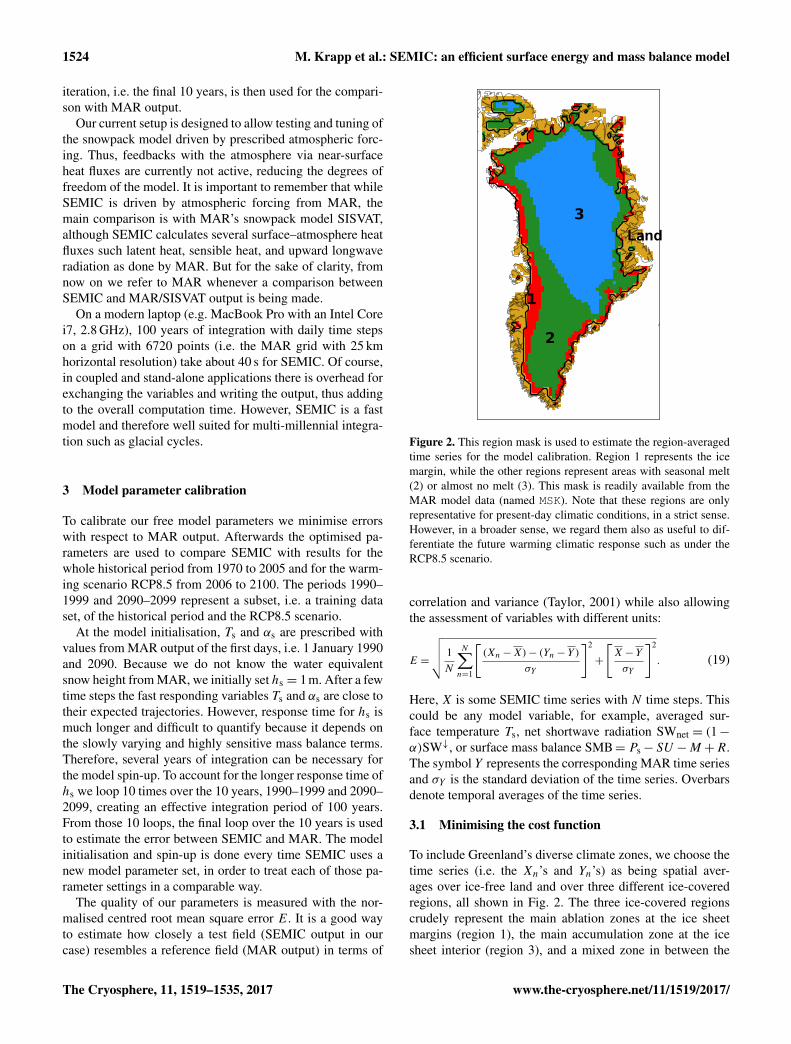
Figure 2. This region mask is used to estimate the region-averagedtime series for the model calibration. Region 1 represents the icemargin, while the other regions represent areas with seasonal melt(2) or almost no melt (3). This mask is readily available from theMAR model data (named MSK). Note that these regions are onlyrepresentative for present-day climatic conditions, in a strict sense.However, in a broader sense, we regard them also as useful to dif-ferentiate the future warming climatic response such as under theRCP8.5 scenario.

correlation and variance (Taylor, 2001) while also allowingthe assessment of variables with different units:

E =

√√√√ 1N

N∑n=1

[(Xn−X)− (Yn−Y )

σY

]2

+

[X−Y

σY

]2

. (19)

Here, X is some SEMIC time series with N time steps. Thiscould be any model variable, for example, averaged sur-face temperature Ts, net shortwave radiation SWnet = (1−α)SW↓, or surface mass balance SMB= Ps−SU −M +R.The symbol Y represents the corresponding MAR time seriesand σY is the standard deviation of the time series. Overbarsdenote temporal averages of the time series.

3.1 Minimising the cost function

To include Greenland’s diverse climate zones, we choose thetime series (i.e. the Xn’s and Yn’s) as being spatial aver-ages over ice-free land and over three different ice-coveredregions, all shown in Fig. 2. The three ice-covered regionscrudely represent the main ablation zones at the ice sheetmargins (region 1), the main accumulation zone at the icesheet interior (region 3), and a mixed zone in between the

The Cryosphere, 11, 1519–1535, 2017 www.the-cryosphere.net/11/1519/2017/

M. Krapp et al.: SEMIC: an efficient surface energy and mass balance model 1525

Table 3. Model parameters with their initial range and their optimal value in bold face.

Symbol Range Value Description

A 0.0–5.0 3.0 amplitude of diurnal cycle [K]αs 0.70–0.90 0.79 fresh dry snow albedoαi 0.25–0.55 0.41 bare ice albedo, i.e. clean or blue iceαl 0.05–0.35 0.07 bare land albedohcrit 0.00–0.20 0.028 critical snow height for albedo parameterisation [m]fR 0.0–1.0 0.85 refreezing correction

main accumulation and ablation zones (region 2). Note, theoutlined regions represent different mass balance zones fortoday’s climate and may change for any future warming sce-nario such as RCP8.5. Nevertheless, the distinction is usefulto derive a differentiated response in each of those regions tothe atmospheric forcing. We calculate four different E val-ues, one over ice-free land (EL) and three over the differentice-covered regions (Eb1, Eb2, Eb3) for both periods, 1990–1999 and 2090–2099, denoted by a subscript, e.g. Ehist

L orE

rcp85b2 .For our cost function we regard the following variables

as important for the surface energy and mass balance: sur-face temperature Ts, net shortwave radiation SWnet, melt M ,and surface mass balance SMB. The magnitude of this vectorthen defines our cost function J ,

J =

∥∥∥∥(EhistL,Ts

,Ehistb1,Ts

, . . .,EhistL,SWnet

, . . .,Ehistb3,SMB,E

rcp85L,Ts

, . . .,Ercp85b3,SMB

)T ∥∥∥∥ , (20)

which we want to minimise. Note that we assign differentarea weights to each of the regions.

The cost function J is minimised with a method calledparticle swarm optimisation (PSO), described below. Us-ing these calibration steps, we derive these optimal pa-rameters values: A= 3.0 K, αs= 0.79, αi = 0.41, αl = 0.07,hcrit= 0.028 m, and fR = 0.85 which are also listed in Ta-ble 3.

3.2 Particle swarm optimisation

Because of the high dimensionality of the parameter space, arandom search for the optimal parameters would need a largesample size on the order ofO(107−8). One optimisation tech-nique that overcomes the problem of large sample sizes isthe so-called particle swarm optimisation (PSO) (Poli et al.,2007). PSO is based on social interaction among particles ofthe “swarm”. Initially, each particle is placed randomly in theparameter space and has a random velocity. For all particlesthe cost function J is calculated (Eq. 20). This determinesthe “fitness” of each individual and of the swarm as a whole.Now, each particle updates its current position and velocityin the parameter space depending on its current and current-best fitness position, and also on the global best-fitness po-sition, with some random perturbations. The next iterationstarts after all particles have moved. Eventually, the swarm

as a whole moves to the minimum of the cost function J . Forour parameter calibration we let 30 particles freely swarmwithin the six-dimensional parameter space. The global best-fitness solution found within 100 iterations1 is then regardedas optimal.

3.3 Calibration results

The ice sheet surface temperature is very well constrained bythe atmospheric forcing fields. Therefore, the surface tem-perature in SEMIC is similar to the one calculated by MAR,as the annual mean differences and the ice sheet averagedtime series show (Figs. 3, 4, 5, and 6). The annual meandifference between SEMIC and MAR for years 1990–1999(2090–2099) is about 0.4 K (0.3 K) over the ice sheet and0.5 K (0.2 K) over ice-free land. While large parts of the icesheet are colder in SEMIC, temperatures at the ice dividesand over ice-free land are generally warmer in SEMIC (seeFigs. 3i and 4i).

The surface mass balance is well captured by SEMIC. Thelargest differences occur in the ablation zones of region 1 and2 around the margin of the ice sheet. While melting2 over thenorthern part of the ice sheet is overestimated by SEMIC,it is underestimated over the southern part of the ice sheet.Nonetheless, for years 1990–1999 (2090–2099) the overallsurface mass balance difference over the ice sheet betweenSEMIC and MAR is almost zero, −0.04 (−0.03) mmday−1,with SEMIC having an average surface mass balance of 1.57(−0.24) mmday−1 and a MAR of 1.61 (−0.21) mmday−1.SEMIC and MAR also exhibit similar melt rates over the icesheet, with differences of −0.06 (−0.15) mmday−1. A de-tailed overview of the differences from the model variablesthat we used to define the cost function is provided in Table 4.

In regions where surface mass balance is positive (seeFigs. 3c, g and 4c, g), errors are small because accumula-tion is mainly prescribed by snowfall and to a lesser extentby sublimation/evaporation. Therefore, differences in abla-tion are more important because they arise dynamically fromSEMIC. The introduced diurnal cycle parameterisation is

1Note, 100 iterations are a predefined upper limit, and solutionsusually tend to converge earlier.

2Note that melt is defined here as a positive quantity but is sub-tracted from the surface mass balance.

www.the-cryosphere.net/11/1519/2017/ The Cryosphere, 11, 1519–1535, 2017

1526 M. Krapp et al.: SEMIC: an efficient surface energy and mass balance model

Table 4. Comparison of SEMIC and MAR. Shown are multi-year mean averages over the ice sheet (regions 1–3) and ice-free land, theirmean grid point to grid point differences 1, their minimum, and their maximum grid point to grid point differences, min1 and max1. Here,ice sheet means all ice-covered regions (region 1–3).

1990–1999 2090–2099SEMIC MAR 1 min1 max1 SEMIC MAR 1 min1 max1

Ice

shee

t Ts [K] 249.6 249.2 1.4 0.2 4.8 256.1 255.8 1.3 0.4 3.7SMB [mmday−1] 1.57 1.61 0.96 −1.78 2.88 −0.24 −0.21 0.97 −2.40 4.70M [mmday−1] 1.62 1.68 0.94 −0.79 3.68 4.05 4.20 0.84 −2.64 4.20SWnet [Wm−2] 28.7 27.7 1.9 −10.9 14.2 31.9 32.0 0.9 −8.7 10.8

Lan

d

Ts [K] 258.4 257.9 1.5 −0.1 5.1 267.5 267.3 1.2 0.0 3.2SMB [mmday−1] 1.27 1.25 1.03 0.67 1.56 1.09 1.00 1.09 0.98 1.87M [mmday−1] 2.18 2.04 1.14 0.60 1.79 2.37 2.25 1.12 0.64 1.44SWnet [Wm−2] 46.8 47.3 0.4 −20.7 22.6 61.7 65.6 −2.9 −13.5 8.3

SEM

IC

(a)

Ts [K]

240

245

250

255

260

265

270

MAR

/Can

ESM

2

(e) 240

245

250

255

260

265

270

SEM

IC -

MAR

/Can

ESM

2

(i) 1.5

1.0

0.5

0.0

0.5

1.0

1.5

SEM

IC

(b)

SWnet [W m 2]

30

40

50

60

70

80

90

MAR

/Can

ESM

2

(f) 30

40

50

60

70

80

90

SEM

IC -

MAR

/Can

ESM

2

(j) 10.07.55.02.5

0.02.55.07.510.0

SEM

IC

(c)

SMB [mm day 1]

108642

024

MAR

/Can

ESM

2

(g) 108642

024

SEM

IC -

MAR

/Can

ESM

2

(k) 1.5

1.0

0.5

0.0

0.5

1.0

1.5

SEM

IC(d)

M [mm day 1]

0

2

4

6

8

10

MAR

/Can

ESM

2

(h) 0

2

4

6

8

10SE

MIC

- M

AR/C

anES

M2

(l) 1.5

1.0

0.5

0.0

0.5

1.0

1.5

Multi-year mean (1990–1999)

Figure 3. Comparison of multi-year (1990–1999) mean surface temperature Ts, net shortwave radiation SWnet, surface mass balance SMB,and surface meltM as modelled by SEMIC (a–d) and MAR (e–h) and the differences between SEMIC and MAR (i–l). The outlined contoursshow the boundaries of the three ice-covered MAR regions as shown in Fig. 2. See Table 4 for values of minimum and maximum differences.

critical here; it allows melting and refreezing within one timestep which would be prohibited otherwise.

SEMIC is able to capture both the increase and decreaseof surface mass balance as well as the seasonal melting as

shown for the different regions and periods in Figs. 5 and6. As can be seen from Fig. 7, errors in melt rates and thesurface mass balance accumulate over time. The calibrationprocedure minimises discrepancies across the four regions

The Cryosphere, 11, 1519–1535, 2017 www.the-cryosphere.net/11/1519/2017/

M. Krapp et al.: SEMIC: an efficient surface energy and mass balance model 1527

SEM

IC

(a)

Ts [K]

240

245

250

255

260

265

270

MAR

/Can

ESM

2

(e) 240

245

250

255

260

265

270

SEM

IC -

MAR

/Can

ESM

2

(i) 1.5

1.0

0.5

0.0

0.5

1.0

1.5

SEM

IC

(b)

SWnet [W m 2]

30

40

50

60

70

80

90

MAR

/Can

ESM

2

(f) 30

40

50

60

70

80

90

SEM

IC -

MAR

/Can

ESM

2

(j) 10.07.55.02.5

0.02.55.07.510.0

SEM

IC

(c)

SMB [mm day 1]

108642

024

MAR

/Can

ESM

2(g) 10

8642

024

SEM

IC -

MAR

/Can

ESM

2

(k) 1.5

1.0

0.5

0.0

0.5

1.0

1.5

SEM

IC

(d)

M [mm day 1]

0

2

4

6

8

10

MAR

/Can

ESM

2

(h) 0

2

4

6

8

10

SEM

IC -

MAR

/Can

ESM

2

(l) 1.5

1.0

0.5

0.0

0.5

1.0

1.5

Multi-year mean (2090–2099)

Figure 4. Comparison of multi-year (2090–2099) mean surface temperature Ts, net shortwave radiation SWnet, surface mass balance SMB,and surface meltM as modelled by SEMIC (a–d) and MAR (e–h) and the differences between SEMIC and MAR (i–l). The outlined contoursshow the boundaries of the three ice-covered MAR regions as shown in Fig. 2. See Table 4 for values of minimum and maximum differences.

and across the two different calibration periods. This resultsin melt rates that are slightly too large in all regions and forboth periods, but the surface mass balance itself is reasonablywell modelled by SEMIC, except for the inner ice sheet re-gion 3 for the years 2090–2099. Overall, using the resultingoptimal parameters from the calibration improves SEMIC’sperformance in modelling the whole historical and RCP8.5period from 1970 to 2099 as shown in the next Sect. 4.

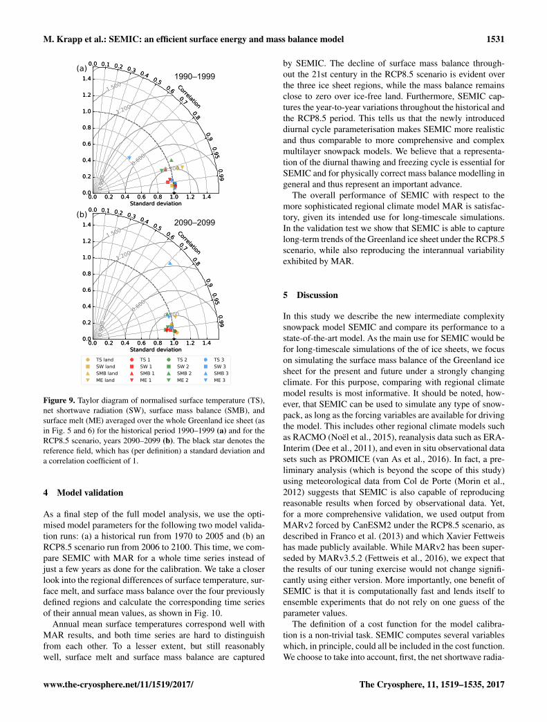
The Taylor diagram in Fig. 9 summarises the performanceof SEMIC compared to MAR’s multilayer snowpack model.Except for the surface mass balance for the RCP8.5 years andthe melt for the historical period in the interior of the Green-land ice sheet (region 3), all variables are reasonably close tothe reference value of each regions’ time series in terms oftheir variability, measured via their standard deviation, andtheir match to the corresponding MAR variables, measuredvia their correlation. A detailed look into each time series(Figs. 5 and 6) further supports our results that SEMIC andMAR variables are reasonably close to each other, especiallyduring the whole melt season.

The overall differences between SEMIC and MAR tem-perature and surface mass balance are small given the chal-lenge of (i) matching both periods, 1990–1999 and 2090–2099, (ii) calibrating different mass and energy-balance vari-ables in parallel, and (iii) using only a subset of grid points(25 %) averaged over four regions across entire Greenland.SEMIC’s annual mean values of surface temperature andsurface mass balance are well suited for applications of in-teractive ice sheet models. The optimisation guarantees thatthe regionally averaged MAR and SEMIC time series are asclose as possible (as defined by the cost function). Never-theless, SEMIC is sensitive to the choice of parameters, sowe now show how perturbed parameters around their opti-mal values affect the surface energy and mass balance of theice sheet.

3.4 Parameter sensitivity

We identified parameters that dominate model uncertaintiesand tested the parameter sensitivity on the model perfor-

www.the-cryosphere.net/11/1519/2017/ The Cryosphere, 11, 1519–1535, 2017

1528 M. Krapp et al.: SEMIC: an efficient surface energy and mass balance model

1990 1995 2000225

250

275

T s

E = 0.08 Land

1990 1995 2000225

250

275E = 0.09 Region 1

1990 1995 2000225

250

275E = 0.11 Region 2

1990 1995 2000225

250

275E = 0.17 Region 3

1990 1995 20000

100

200

SWne

t

E = 0.10

1990 1995 20000

100

200E = 0.16

1990 1995 20000

100

200E = 0.13

1990 1995 20000

100

200E = 0.12

1990 1995 2000

20

0

SMB

E = 0.32

1990 1995 2000

20

0

E = 0.31

1990 1995 2000

20

0

E = 0.42

1990 1995 2000

20

0

E = 0.07

1990 1995 2000

2

0

2

h s

E = 0.45

1990 1995 2000

2

0

2E = 0.34

1990 1995 2000

2

0

2E = 0.52

1990 1995 2000

2

0

2E = 1.37

1990 1995 20000

20

M

E = 0.34

1990 1995 20000

20

E = 0.18

1990 1995 20000

20

E = 0.33

1990 1995 20000

20

E = 0.72

1990 1995 20000

5R

E = 0.62

1990 1995 20000

5

E = 0.59

1990 1995 20000

5

E = 0.49

1990 1995 20000

5

E = 0.80

1990 1995 2000

0

20

HL

E = 0.39

1990 1995 2000

0

20

E = 1.06

1990 1995 2000

0

20

E = 1.83

1990 1995 2000

0

20

E = 2.00

1990 1995 2000Time

50

0

50

HS

E = 0.38

SEMIC MAR/CanESM2

1990 1995 2000Time

50

0

50E = 0.78

1990 1995 2000Time

50

0

50E = 0.72

1990 1995 2000Time

50

0

50E = 1.05

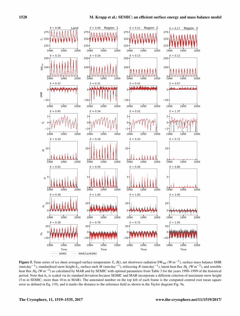
Figure 5. Time series of ice sheet averaged surface temperature Ts (K), net shortwave radiation SWnet (Wm−2), surface mass balance SMB(mmday−1), standardised snow height hs, surface meltM (mmday−1), refreezing R (mmday−1), latent heat fluxHL (Wm−2), and sensibleheat flux HS (Wm−2) as calculated by MAR and by SEMIC with optimal parameters from Table 3 for the years 1990–1999 of the historicalperiod. Note that hs is scaled via its standard deviation because SEMIC and MAR incorporate a different criterion of maximum snow height(5 m in SEMIC; more than 10 m in MAR). The annotated number on the top left of each frame is the computed centred root mean squareerror as defined in Eq. (19), and it marks the distance to the reference field as shown in the Taylor diagram Fig. 9a.

The Cryosphere, 11, 1519–1535, 2017 www.the-cryosphere.net/11/1519/2017/

M. Krapp et al.: SEMIC: an efficient surface energy and mass balance model 1529

2090 2095 2100225

250

275

T s

E = 0.09 Land

2090 2095 2100225

250

275

E = 0.10 Region 1

2090 2095 2100225

250

275

E = 0.10 Region 2

2090 2095 2100225

250

275

E = 0.15 Region 3

2090 2095 21000

100

200

SWne

t

E = 0.19

2090 2095 21000

100

200

E = 0.12

2090 2095 21000

100

200

E = 0.16

2090 2095 21000

100

200

E = 0.16

2090 2095 2100

50

25

0

SMB

E = 0.19

2090 2095 2100

50

25

0E = 0.16

2090 2095 2100

50

25

0E = 0.32

2090 2095 2100

50

25

0E = 0.97

2090 2095 2100

2

0

2

h s

E = 0.25

2090 2095 2100

2

0

2E = 0.41

2090 2095 2100

2

0

2E = 0.28

2090 2095 2100

2

0

2E = 0.58

2090 2095 21000

25

50

M

E = 0.28

2090 2095 21000

25

50

E = 0.14

2090 2095 21000

25

50

E = 0.17

2090 2095 21000

25

50

E = 0.28

2090 2095 21000

5

10

R

E = 0.73

2090 2095 21000

5

10

E = 0.50

2090 2095 21000

5

10

E = 0.57

2090 2095 21000

5

10

E = 0.48

2090 2095 2100

0

50

HL

E = 0.30

2090 2095 2100

0

50

E = 0.68

2090 2095 2100

0

50

E = 1.76

2090 2095 2100

0

50

E = 2.38

2090 2095 2100Time

100

0

HS

E = 0.35

SEMIC MAR/CanESM2

2090 2095 2100Time

100

0

E = 0.88

2090 2095 2100Time

100

0

E = 0.79

2090 2095 2100Time

100

0

E = 0.98

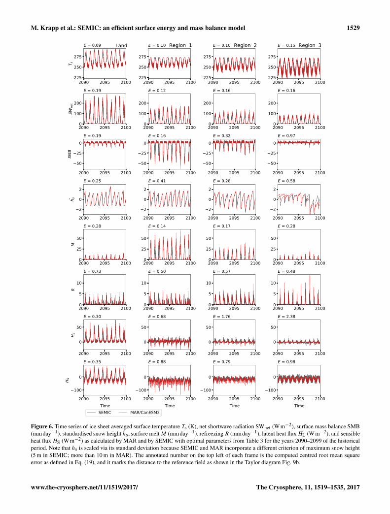
Figure 6. Time series of ice sheet averaged surface temperature Ts (K), net shortwave radiation SWnet (Wm−2), surface mass balance SMB(mmday−1), standardised snow height hs, surface meltM (mmday−1), refreezing R (mmday−1), latent heat fluxHL (Wm−2), and sensibleheat flux HS (Wm−2) as calculated by MAR and by SEMIC with optimal parameters from Table 3 for the years 2090–2099 of the historicalperiod. Note that hs is scaled via its standard deviation because SEMIC and MAR incorporate a different criterion of maximum snow height(5 m in SEMIC; more than 10 m in MAR). The annotated number on the top left of each frame is the computed centred root mean squareerror as defined in Eq. (19), and it marks the distance to the reference field as shown in the Taylor diagram Fig. 9b.

www.the-cryosphere.net/11/1519/2017/ The Cryosphere, 11, 1519–1535, 2017

1530 M. Krapp et al.: SEMIC: an efficient surface energy and mass balance model

1990 1995 2000

0

1000

2000

3000

Cum

. mas

s [Gt

]

(a) Land

1990 1995 2000

5000

0

5000

10 000

Cum

. mas

s [Gt

]

(b) Region 1

1990 2000

0

1000

2000

3000

Cum

. mas

s [Gt

]

(c) Region 3

1990 20001995Time (years)

5000

0

5000

10 000 Cu

m. m

ass [

Gt]

(d) Region 2

2090 2095 2100

0

1000

2000

3000

Cum

. mas

s [Gt

]

(e) Land

2090 2095 2100

5000

0

5000

10 000

Cum

. mas

s [Gt

]

(f) Region 1

2090 2100

0

1000

2000

3000

Cum

. mas

s [Gt

]

(g) Region 3

Surface mass balanceSEMICMAR/CanESM

Surface meltSEMICMAR/CanESM2

2090 2100

5000

0

5000

10 000

Cum

. mas

s [Gt

]

(h) Region 2

1995Time (years)

1995Time (years)

1995Time (years)

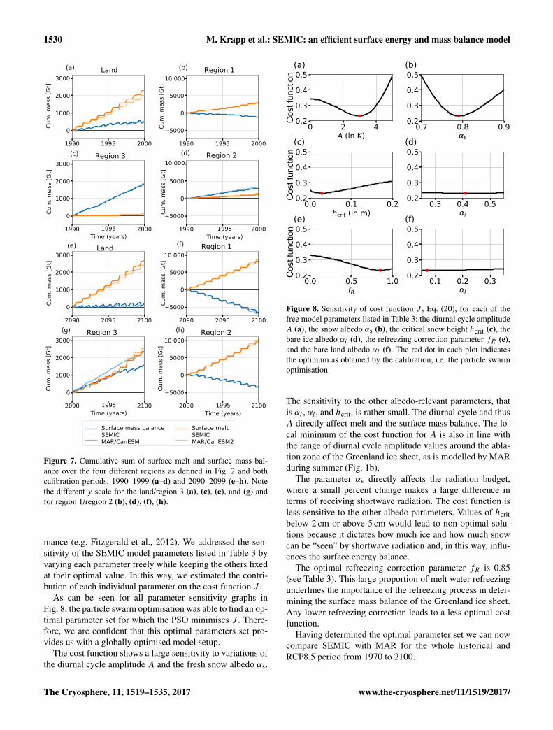
Figure 7. Cumulative sum of surface melt and surface mass bal-ance over the four different regions as defined in Fig. 2 and bothcalibration periods, 1990–1999 (a–d) and 2090–2099 (e–h). Notethe different y scale for the land/region 3 (a), (c), (e), and (g) andfor region 1/region 2 (b), (d), (f), (h).

mance (e.g. Fitzgerald et al., 2012). We addressed the sen-sitivity of the SEMIC model parameters listed in Table 3 byvarying each parameter freely while keeping the others fixedat their optimal value. In this way, we estimated the contri-bution of each individual parameter on the cost function J .

As can be seen for all parameter sensitivity graphs inFig. 8, the particle swarm optimisation was able to find an op-timal parameter set for which the PSO minimises J . There-fore, we are confident that this optimal parameters set pro-vides us with a globally optimised model setup.

The cost function shows a large sensitivity to variations ofthe diurnal cycle amplitude A and the fresh snow albedo αs.

0 2 4A (in K)

0.20.30.40.5

Cos

t fun

ctio

n

(a)

0.7 0.8 0.9s

0.20.30.40.5(b)

0.0 0.1 0.2hcrit (in m)

0.20.30.40.5

Cos

t fun

ctio

n

(c)

0.3 0.4 0.5i

0.20.30.40.5(d)

0.0 0.5 1.0fR

0.20.30.40.5

Cos

t fun

ctio

n

(e)

0.1 0.2 0.3l

0.20.30.40.5(f)

Figure 8. Sensitivity of cost function J , Eq. (20), for each of thefree model parameters listed in Table 3: the diurnal cycle amplitudeA (a), the snow albedo αs (b), the critical snow height hcrit (c), thebare ice albedo αi (d), the refreezing correction parameter fR (e),and the bare land albedo αl (f). The red dot in each plot indicatesthe optimum as obtained by the calibration, i.e. the particle swarmoptimisation.

The sensitivity to the other albedo-relevant parameters, thatis αi , αl , and hcrit, is rather small. The diurnal cycle and thusA directly affect melt and the surface mass balance. The lo-cal minimum of the cost function for A is also in line withthe range of diurnal cycle amplitude values around the abla-tion zone of the Greenland ice sheet, as is modelled by MARduring summer (Fig. 1b).

The parameter αs directly affects the radiation budget,where a small percent change makes a large difference interms of receiving shortwave radiation. The cost function isless sensitive to the other albedo parameters. Values of hcritbelow 2 cm or above 5 cm would lead to non-optimal solu-tions because it dictates how much ice and how much snowcan be “seen” by shortwave radiation and, in this way, influ-ences the surface energy balance.

The optimal refreezing correction parameter fR is 0.85(see Table 3). This large proportion of melt water refreezingunderlines the importance of the refreezing process in deter-mining the surface mass balance of the Greenland ice sheet.Any lower refreezing correction leads to a less optimal costfunction.

Having determined the optimal parameter set we can nowcompare SEMIC with MAR for the whole historical andRCP8.5 period from 1970 to 2100.

The Cryosphere, 11, 1519–1535, 2017 www.the-cryosphere.net/11/1519/2017/

M. Krapp et al.: SEMIC: an efficient surface energy and mass balance model 1531

0.0 0.1 0.2 0.3 0.4 0.50.6

0.7

0.80.9

0.950.99

Correlation

0.0 0.2 0.4 0.6 0.8 1.0 1.2 1.4Standard deviation

0.0

0.2

0.4

0.6

0.8

1.0

1.2

1.4

0.0 0.1 0.2 0.3 0.4 0.50.6

0.7

0.80.9

0.950.99

Correlation

0.0 0.2 0.4 0.6 0.8 1.0 1.2 1.4Standard deviation

0.0

0.2

0.4

0.6

0.8

1.0

1.2

1.4 1990–1999(a)

1.500

0.300

1.200

0.600

0.90

0

0.0 0.1 0.2 0.3 0.4 0.50.6

0.7

0.80.9

0.950.99

Correlation

0.0 0.2 0.4 0.6 0.8 1.0 1.2 1.4Standard deviation

0.0

0.2

0.4

0.6

0.8

1.0

1.2

1.4

0.0 0.1 0.2 0.3 0.4 0.50.6

0.7

0.80.9

0.950.99

Correlation

0.0 0.2 0.4 0.6 0.8 1.0 1.2 1.4Standard deviation

0.0

0.2

0.4

0.6

0.8

1.0

1.2

1.4 2090–2099(b)

0.300

0.90

0

1.500

1.200

0.600

TS landSW landSMB landME land

TS 1SW 1SMB 1ME 1

TS 2SW 2SMB 2ME 2

TS 3SW 3SMB 3ME 3

Figure 9. Taylor diagram of normalised surface temperature (TS),net shortwave radiation (SW), surface mass balance (SMB), andsurface melt (ME) averaged over the whole Greenland ice sheet (asin Fig. 5 and 6) for the historical period 1990–1999 (a) and for theRCP8.5 scenario, years 2090–2099 (b). The black star denotes thereference field, which has (per definition) a standard deviation anda correlation coefficient of 1.

4 Model validation

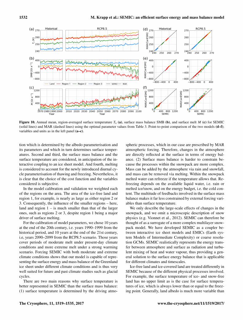
As a final step of the full model analysis, we use the opti-mised model parameters for the following two model valida-tion runs: (a) a historical run from 1970 to 2005 and (b) anRCP8.5 scenario run from 2006 to 2100. This time, we com-pare SEMIC with MAR for a whole time series instead ofjust a few years as done for the calibration. We take a closerlook into the regional differences of surface temperature, sur-face melt, and surface mass balance over the four previouslydefined regions and calculate the corresponding time seriesof their annual mean values, as shown in Fig. 10.

Annual mean surface temperatures correspond well withMAR results, and both time series are hard to distinguishfrom each other. To a lesser extent, but still reasonablywell, surface melt and surface mass balance are captured

by SEMIC. The decline of surface mass balance through-out the 21st century in the RCP8.5 scenario is evident overthe three ice sheet regions, while the mass balance remainsclose to zero over ice-free land. Furthermore, SEMIC cap-tures the year-to-year variations throughout the historical andthe RCP8.5 period. This tells us that the newly introduceddiurnal cycle parameterisation makes SEMIC more realisticand thus comparable to more comprehensive and complexmultilayer snowpack models. We believe that a representa-tion of the diurnal thawing and freezing cycle is essential forSEMIC and for physically correct mass balance modelling ingeneral and thus represent an important advance.

The overall performance of SEMIC with respect to themore sophisticated regional climate model MAR is satisfac-tory, given its intended use for long-timescale simulations.In the validation test we show that SEMIC is able to capturelong-term trends of the Greenland ice sheet under the RCP8.5scenario, while also reproducing the interannual variabilityexhibited by MAR.

5 Discussion

In this study we describe the new intermediate complexitysnowpack model SEMIC and compare its performance to astate-of-the-art model. As the main use for SEMIC would befor long-timescale simulations of the of ice sheets, we focuson simulating the surface mass balance of the Greenland icesheet for the present and future under a strongly changingclimate. For this purpose, comparing with regional climatemodel results is most informative. It should be noted, how-ever, that SEMIC can be used to simulate any type of snow-pack, as long as the forcing variables are available for drivingthe model. This includes other regional climate models suchas RACMO (Noël et al., 2015), reanalysis data such as ERA-Interim (Dee et al., 2011), and even in situ observational datasets such as PROMICE (van As et al., 2016). In fact, a pre-liminary analysis (which is beyond the scope of this study)using meteorological data from Col de Porte (Morin et al.,2012) suggests that SEMIC is also capable of reproducingreasonable results when forced by observational data. Yet,for a more comprehensive validation, we used output fromMARv2 forced by CanESM2 under the RCP8.5 scenario, asdescribed in Franco et al. (2013) and which Xavier Fettweishas made publicly available. While MARv2 has been super-seded by MARv3.5.2 (Fettweis et al., 2016), we expect thatthe results of our tuning exercise would not change signifi-cantly using either version. More importantly, one benefit ofSEMIC is that it is computationally fast and lends itself toensemble experiments that do not rely on one guess of theparameter values.

The definition of a cost function for the model calibra-tion is a non-trivial task. SEMIC computes several variableswhich, in principle, could all be included in the cost function.We choose to take into account, first, the net shortwave radia-

www.the-cryosphere.net/11/1519/2017/ The Cryosphere, 11, 1519–1535, 2017

1532 M. Krapp et al.: SEMIC: an efficient surface energy and mass balance model

240 250 260 270240

250

260

270

MAR

/Can

ESM

2

(d) Historical

240 250 260 270240

250

260

270 RCP8.5

800 400 0 400800

400

0

400

MAR

/Can

ESM

2

(e)

800 400 0 400800

400

0

400

0 400 800 1200SEMIC

0

400

800

1200

MAR

/Can

ESM

2

(f)

0 400 800 1200SEMIC

0

400

800

1200

MAR

/Can

ESM

2

240

250

260

270T s

[K]

(a) Historical RCP8.5

800

400

0

400

SMB

[Gt a

1 ]

(b)

Land Region 1 Region 2 Region 3

1970 1980 1990 2000Year

0

400

800

1200

M [G

t a1 ]

(c)

2010 2020 2030 2040 2050 2060 2070 2080 2090 2100Year

SEMIC MAR

Figure 10. Annual mean, region-averaged surface temperature Ts (a), surface mass balance SMB (b), and surface melt M (c) for SEMIC(solid lines) and MAR (dashed lines) using the optimal parameter values from Table 3. Point-to-point comparison of the two models (d–f);variables and units as in the left panel (a–c).

tion which is determined by the albedo parameterisation andits parameters and which in turn determines surface temper-atures. Second and third, the surface mass balance and thesurface temperature are considered, in anticipation of the in-teractive coupling to an ice sheet model. And fourth, meltingis considered to account for the newly introduced diurnal cy-cle parameterisation of thawing and freezing. Nevertheless, itis clear that the choice of the cost function and the variablesconsidered is subjective.

In the model calibration and validation we weighted eachof the regions on the area. The area of the ice-free land andregion 1, for example, is nearly as large as either region 2 or3. Consequently, the influence of the smaller regions – here,land and region 1 – is much smaller than that of the largerones, such as regions 2 or 3, despite region 1 being a majordriver of surface melting.

For the calibration of model parameters, we chose 10 yearsat the end of the 20th century, i.e. years 1990–1999 from thehistorical period, and 10 years at the end of the 21st century,i.e, years 2090–2099 from the RCP8.5 scenario. Those yearscover periods of moderate melt under present-day climateconditions and more extreme melt under a strong warmingscenario. Forcing SEMIC with both moderate and extremeclimate conditions shows that our model is capable of repre-senting the surface energy and mass balance of the Greenlandice sheet under different climate conditions and is thus verywell suited for future and past climate studies such as glacialcycles.

There are two main reasons why surface temperature isbetter represented in SEMIC than the surface mass balance:(1) surface temperature is determined by the driving atmo-

spheric processes, which in our case are prescribed by MARatmospheric forcing. Therefore, changes in the atmosphereare directly reflected at the surface in terms of energy bal-ance. (2) Surface mass balance is harder to constrain be-cause the processes within the snowpack are more complex.Mass can be added by the atmosphere via rain and snowfall,and mass can be removed via melting. Within the snowpackmelted water can refreeze if the temperature allows that. Re-freezing depends on the available liquid water, i.e. rain ormelted ice/snow, and on the energy budget, i.e. the cold con-tent. The multitude of feedbacks involved in the surface massbalance makes it far less constrained by external forcing vari-ables than surface temperature.

We only describe the large-scale effects of changes in thesnowpack, and we omit a microscopic description of snowphysics (e.g. Vionnet et al., 2012). SEMIC can therefore bethought of as a surrogate of a more complex multilayer snow-pack model. We have developed SEMIC as a coupler be-tween interactive ice sheet models and EMICs (Earth sys-tem Models of Intermediate Complexity) or coarse resolu-tion GCMs. SEMIC realistically represents the energy trans-fer between atmosphere and surface as radiation and turbu-lent mixing of heat and water vapour, thus providing a gen-eral solution to the surface energy balance that is applicablefor different climates and timescales.

Ice-free land and ice-covered land are treated differently inSEMIC because of the different physical processes involved.For example, the surface temperature of ice- and snow-freeland has no upper limit as is the case for surface tempera-tures of ice, which is always lower than or equal to the freez-ing point. Generally, land albedo is much more variable than

The Cryosphere, 11, 1519–1535, 2017 www.the-cryosphere.net/11/1519/2017/

M. Krapp et al.: SEMIC: an efficient surface energy and mass balance model 1533

as described by the single bare land albedo used in SEMIC.Different land and vegetation types have different effects onthe radiation budget. Consequently, net shortwave radiationerrors in SEMIC are larger over ice-free land than over theice sheet (Figs. 3j and 4j).

Details in model representation also reveal differences be-tween SEMIC and MAR. However, these differences are notso much related to the underlying physical principles, i.e. theassumption of energy and mass balance of the snow- and ice-covered surface, as to the choice of parameters made in orderto match SEMIC variables to MAR variables.

SEMIC makes use of two simple but effective parameter-isations that are important for its good performance: one isthe surface albedo for which we already discussed the prob-lem of the net shortwave radiation budget over ice-free land.Although the net shortwave radiation has an effect on thesurface energy balance, errors do not translate directly intoerrors in the surface temperature (Figs. 3i and 4i). One rea-son is that the contribution of sensible and latent heat fluxis larger over ice-free land is because of the larger tempera-ture contrast. Latent heat flux, for example, is about 10-timeslarger over ice-free land than over the ice sheet.

Another reason for SEMIC’s good performance is thenewly introduced diurnal cycle parameterisation, which al-lows for faster computation while adding the daily thaw–freeze cycle during melt season. The representation of thediurnal cycle of the whole ice sheet by a single constant valueis somewhat problematic because in reality, it changes overtime and location, depending on the climatic conditions, e.g.cloud cover and its effect on downwelling longwave radia-tion. Nevertheless, the overall results of SEMIC with respectto surface mass balance are satisfactory. The diurnal cycleopens many new aspects which could improve model results,e.g. a spatial dependence such as height-dependent ampli-tude or a direct calculation of the amplitude by the coupledatmospheric model, but this is beyond the scope of this paper.Also, a different or a more realistic albedo scheme could re-place the current simple albedo parameterisation (Oerlemansand Knap, 1998). SEMIC has also been successfully testedwith a temperature-dependent albedo scheme (Slater et al.,1998).

Our results underpin the consistent representation of thedominant processes involved in the complex interactions be-tween snow- or ice-covered surfaces and the atmosphere.SEMIC incorporates simpler dynamics compared to multi-layer snowpack models, but represents the essential surfaceenergy and mass balance processes, and is still fast in termsof computational time.

SEMIC is well suited for long-term integrations up to sev-eral millennia and has been successfully tested for the last78 000 years (data taken from Heinemann et al., 2014, per-sonal communication). From the 100 year runtime estimatewe can assume that computation of the surface mass balanceon every single day during one glacial cycle (of about 100 kyears) would take about 11 h. Current state-of-the-art mul-

tilayer snowpack models are not able to perform such longintegrations, but they also do not serve this purpose. Underthese circumstances, using a much simpler model – such asSEMIC – is advised.

SEMIC is well suited for applications with global climatemodels which have just started to master glacial timescales(e.g. Heinemann et al., 2014). SEMIC will be part of thenext version of the regional energy and moisture and balancemodel (REMBO; Robinson et al., 2010) and is also ready tobe coupled to an interactive ice sheet model (Krapp, 2017c).SEMIC is considered as an open-source project, thereforecontributions are welcome, and we encourage and supportthe integration of SEMIC into climate and ice sheet models.

6 Conclusions

We have presented a new Surface Energy and Mass bal-ance model of Intermediate Complexity for snow- and ice-covered surfaces that is simple and fast enough for long-term integrations up to glacial timescales. SEMIC is a physi-cally based model that accounts for energy and mass balanceand it can be used as a surrogate for computationally inten-sive regional climate models with their multilayer snowpackmodels. The most important features of SEMIC are a sim-ple but effective surface albedo parameterisation and a pa-rameterisation of the daily thaw–freeze cycle that allows par-titioning between melting and refreezing. SEMIC has beenforced with atmospheric fields from the regional climatemodel MAR (MARv2) and compared to MAR’s multilayersnowpack model SISVAT; SEMIC represents surface temper-ature and surface mass balance considerably well. For theRCP8.5 warming scenario, SEMIC correctly simulates theclimatological trend and the interannual variability of surfacetemperature and the mass balance of the ice sheet. SEMIChereby incorporates a minimum number of free model pa-rameters, and a large effort was made to balance the com-plexity of the represented processes in favour of faster com-putation.

Data availability. We hereby acknowledge, support, and encour-age research that follows standards with respect to scientific re-producibility, transparency, and data availability. Any model sourcecode and the authors’ manuscript source (typeset in LaTeX) is freelyavailable and accessible online.

The project infrastructure covering individual steps starting fromdata download and preparation, model source code compilation,running the optimisation, running the calibrated model, runningthe model with historical and RCP8.5 scenario data, as well asthe source code of the manuscript with its figures can be down-loaded from the repository website https://gitlab.pik-potsdam.de/krapp/semic-project. See the project website’s README.md for de-tails. The project can also be cloned using git:git clone -b v1.1

www.the-cryosphere.net/11/1519/2017/ The Cryosphere, 11, 1519–1535, 2017

1534 M. Krapp et al.: SEMIC: an efficient surface energy and mass balance model

git@gitlab.pik-potsdam.de:krapp/semic-project.git

The atmospheric forcing data from the MAR/CanESM2 modelfor the historical period from 1970 to 2005 and for the RCP8.5 sce-nario for the period from 2005 to 2100 are available atftp://ftp.climato.be/fettweis/MARv2/.

Author contributions. MK, AR, and AG designed the model. MKimplemented the model code with contributions from AR. MK im-plemented and carried out the model calibration and the data anal-ysis. MK prepared the manuscript with contributions from all co-authors.

Competing interests. The authors declare that they have no conflictof interest.

Acknowledgements. We would like to thank Xavier Fettweis forproviding MAR/CanESM2 data. Mario Krapp is also grateful toMalte Heinemann and Axel Timmermann for their kind hospitalityduring his research visit at the International Pacific ResearchCenter (SOEST, University of Hawaii). Alexander Robinson wasfunded by the Marie Curie 7th Framework Programme (ProjectPIEF-GA-2012-331835, EURICE). Mario Krapp was funded bythe Deutsche Forschungsgemeinschaft (DFG) Project “Modelingthe Greenland ice sheet response to climate change on differenttimescales”.

Edited by: Marco TedescoReviewed by: Xavier Fettweis and one anonymous referee

References

Bougamont, M., Bamber, J., Ridley, J., Gladstone, R., Greuell,W., Hanna, E., Payne, A., and Rutt, I.: Impact of modelphysics on estimating the surface mass balance of theGreenland ice sheet, Geophys. Res. Lett., 34, L17501,https://doi.org/10.1029/2007GL030700, 2007.

Calov, R., Ganopolski, A., Claussen, M., Petoukhov, V., and Greve,R.: Transient simulation of the last glacial inception, Part I:glacial inception as a bifurcation in the climate system, Clim. Dy-nam., 24, 545–561, https://doi.org/10.1007/s00382-005-0007-6,2005.

Cuffey, K. and Paterson, W. S. B.: The Physics of Glaciers, Elsevier,4th edn., 2010.

Dee, D. P., Uppala, S. M., Simmons, A. J., Berrisford, P., Poli,P., Kobayashi, S., Andrae, U., Balmaseda, M. A., Balsamo, G.,Bauer, P., Bechtold, P., Beljaars, A. C. M., van de Berg, L., Bid-lot, J., Bormann, N., Delsol, C., Dragani, R., Fuentes, M., Geer,A. J., Haimberger, L., Healy, S. B., Hersbach, H., Hólm, E. V.,Isaksen, L., Kållberg, P., Köhler, M., Matricardi, M., McNally,A. P., Monge-Sanz, B. M., Morcrette, J.-J., Park, B.-K., Peubey,C., de Rosnay, P., Tavolato, C., Thépaut, J.-N., and Vitart, F.: TheERA-Interim reanalysis: configuration and performance of thedata assimilation system, Q. J. Roy. Meteor. Soc., 137, 553–597,https://doi.org/10.1002/qj.828, 2011.

Fettweis, X., Franco, B., Tedesco, M., van Angelen, J. H., Lenaerts,J. T. M., van den Broeke, M. R., and Gallée, H.: Estimatingthe Greenland ice sheet surface mass balance contribution to fu-ture sea level rise using the regional atmospheric climate modelMAR, The Cryosphere, 7, 469–489, https://doi.org/10.5194/tc-7-469-2013, 2013.

Fettweis, X., Box, J. E., Agosta, C., Amory, C., Kittel, C., Lang, C.,van As, D., Machguth, H., and Gallée, H.: Reconstructions of the1900–2015 Greenland ice sheet surface mass balance using theregional climate MAR model, The Cryosphere, 11, 1015–1033,https://doi.org/10.5194/tc-11-1015-2017, 2017.

Fitzgerald, P. W., Bamber, J. L., Ridley, J. K., and Rougier, J. C.:Exploration of parametric uncertainty in a surface mass balancemodel applied to the Greenland ice sheet, J. Geophys. Res., 117,F01021, https://doi.org/10.1029/2011JF002067, 2012.

Franco, B., Fettweis, X., and Erpicum, M.: Future projections of theGreenland ice sheet energy balance driving the surface melt, TheCryosphere, 7, 1–18, https://doi.org/10.5194/tc-7-1-2013, 2013.

Gill, A. E.: Atmosphere-Ocean Dynamics, International Geo-physics Series, Academic Press, New York, Vol. 30, 1982.

Greuell, W., Genthon, C., and Houghton, J.: Modelling land-icesurface mass balance, Cambridge University Press, 117–168,https://doi.org/10.1017/CBO9780511535659.007, 2004.

Hanna, E., Navarro, F. J., Pattyn, F., Domingues, C. M., Fet-tweis, X., Ivins, E. R., Nicholls, R. J., Ritz, C., Smith,B., Tulaczyk, S., Whitehouse, P. L., and Zwally, H. J.: Ice-sheet mass balance and climate change, Nature, 498, 51–59,https://doi.org/10.1038/nature12238, 2013.

Heinemann, M., Timmermann, A., Elison Timm, O., Saito, F.,and Abe-Ouchi, A.: Deglacial ice sheet meltdown: orbitalpacemaking and CO2 effects, Clim. Past, 10, 1567–1579,https://doi.org/10.5194/cp-10-1567-2014, 2014.

Krapp, M.: Model Code, https://doi.org/10.17605/OSF.IO/5PUX2,last access: 16 May 2017a.

Krapp, M.: Model Data, https://doi.org/10.17605/OSF.IO/A3VH2,16 May 2017b.

Krapp, M.: SEMIC: Surface Energy and mass balance model ofintermediate complexity, GitHub repository, available at: https://github.com/mkrapp/semic, 2017c.

Morin, S., Lejeune, Y., Lesaffre, B., Panel, J.-M., Poncet, D., David,P., and Sudul, M.: An 18-yr long (1993–2011) snow and meteo-rological dataset from a mid-altitude mountain site (Col de Porte,France, 1325 m alt.) for driving and evaluating snowpack mod-els, Earth Syst. Sci. Data, 4, 13–21, https://doi.org/10.5194/essd-4-13-2012, 2012.

Moss, R. H., Edmonds, J. A., Hibbard, K. A., Manning, M. R., Rose,S. K., van Vuuren, D. P., Carter, T. R., Emori, S., Kainuma, M.,Kram, T., Meehl, G. A., Mitchell, J. F. B., Nakicenovic, N., Ri-ahi, K., Smith, S. J., Stouffer, R. J., Thomson, A. M., Weyant,J. P., and Wilbanks, T. J.: The next generation of scenarios forclimate change research and assessment, Nature, 463, 747–756,https://doi.org/10.1038/nature08823, 2010.

Nghiem, S. V., Hall, D. K., Mote, T. L., Tedesco, M., Al-bert, M. R., Keegan, K., Shuman, C. A., DiGirolamo, N. E.,and Neumann, G.: The extreme melt across the Green-land ice sheet in 2012, Geophys. Res. Lett., 39, L20502,https://doi.org/10.1029/2012GL053611, 2012.

Noël, B., van de Berg, W. J., van Meijgaard, E., Kuipers Munneke,P., van de Wal, R. S. W., and van den Broeke, M. R.: Evalua-

The Cryosphere, 11, 1519–1535, 2017 www.the-cryosphere.net/11/1519/2017/

M. Krapp et al.: SEMIC: an efficient surface energy and mass balance model 1535

tion of the updated regional climate model RACMO2.3: summersnowfall impact on the Greenland Ice Sheet, The Cryosphere, 9,1831–1844, https://doi.org/10.5194/tc-9-1831-2015, 2015.

Oerlemans, J.: The mass balance of the Greenland icesheet: sensitivity to climate change as revealed byenergy-balance modelling, The Holocene, 1, 40–48,https://doi.org/10.1177/095968369100100106, 1991.

Oerlemans, J. and Knap, W.: A 1 year record of global radiation andalbedo in the ablation zone of Morteratschgletscher, Switzerland,J. Glaciol., 44, 231–238, https://doi.org/10.3198/1998JoG44-147-231-238, 1998.

Ohmura, A.: Physical Basis for the Temperature-Based Melt-Index Method, J. Appl. Meteo-rol., 40, 753–761, https://doi.org/10.1175/1520-0450(2001)040<0753:PBFTTB>2.0.CO;2, 2001.

Poli, R., Kennedy, J., and Blackwell, T.: Particleswarm optimization, Swarm Intelligence, 1, 33–57,https://doi.org/10.1007/s11721-007-0002-0, 2007.

Reeh, N.: Parameterization of melt rate and surface temperature onthe Greenland ice sheet, Polarforschung, 59, 113–128, 1991.

Reijmer, C. H., van den Broeke, M. R., Fettweis, X., Ettema,J., and Stap, L. B.: Refreezing on the Greenland ice sheet: acomparison of parameterizations, The Cryosphere, 6, 743–762,https://doi.org/10.5194/tc-6-743-2012, 2012.

Robinson, A. and Goelzer, H.: The importance of insolationchanges for paleo ice sheet modeling, The Cryosphere, 8, 1419–1428, https://doi.org/10.5194/tc-8-1419-2014, 2014.

Robinson, A., Calov, R., and Ganopolski, A.: An efficient regionalenergy-moisture balance model for simulation of the GreenlandIce Sheet response to climate change, The Cryosphere, 4, 129–144, https://doi.org/10.5194/tc-4-129-2010, 2010.

Slater, A., Pitman, A., and Desborough, C.: The vali-dation of a snow parameterization designed for usein general circulation models, International J. Clima-tol., 18, 595–617, https://doi.org/10.1002/(SICI)1097-0088(199805)18:6<595::AID-JOC275>3.0.CO;2-O, 1998.

Taylor, K. E.: Summarizing multiple aspects of model performancein a single diagram, J. Geophys. Res.-Atmos., 106, 7183–7192,https://doi.org/10.1029/2000JD900719, 2001.

Thomas, R., Frederick, E., Li, J., Krabill, W., Manizade, S., Paden,J., Sonntag, J., Swift, R., and Yungel, J.: Accelerating ice lossfrom the fastest Greenland and Antarctic glaciers, Geophys. Res.Lett., 38, L10502, https://doi.org/10.1029/2011GL047304, 2011.

van As, D., Fausto, R. S., Cappelen, J., van de Wal, R. S., Braith-waite, R. J., Machguth, H., Charalampidis, C., Box, J. E., Sol-gaard, A. M., Ahlstrøm, A. P., Haubner, K., Citterio M., and An-dersen, S. B.: Placing Greenland ice sheet ablation measurementsin a multi-decadal context, Geol. Surv. Denm. Greenl., 35, 71–74, 2016.

van de Berg, W., van den Broeke, M., Ettema, J., van Meijgaard, E.,and Kaspar, F.: Significant contribution of insolation to Eemianmelting of the Greenland ice sheet, Nat. Geosci., 4, 679–683,https://doi.org/10.1038/ngeo1245, 2011.

van den Broeke, M., Bamber, J., Ettema, J., Rignot, E., Schrama, E.,van de Berg, W., van Meijgaard, E., Velicogna, I., and Wouters,B.: Partitioning Recent Greenland Mass Loss, Science, 326, 984–986, https://doi.org/10.1126/science.1178176, 2009.

Vionnet, V., Brun, E., Morin, S., Boone, A., Faroux, S., Le Moigne,P., Martin, E., and Willemet, J.-M.: The detailed snowpackscheme Crocus and its implementation in SURFEX v7.2, Geosci.Model Dev., 5, 773–791, https://doi.org/10.5194/gmd-5-773-2012, 2012.

www.the-cryosphere.net/11/1519/2017/ The Cryosphere, 11, 1519–1535, 2017