semi-markov model for market microstructure and hf...

Introduction Semi Markov model for microstructure price Market making Conclusion

Semi-Markov model formarket microstructure and HF trading

Huyen PHAM

LPMA, University Paris Diderotand JVN Institute, VNU, Ho-Chi-Minh City

NUS-UTokyo Workshop on Quantitative FinanceSingapore, 26-27 september 2013

Joint work with Pietro FODRAEXQIM and LPMA, University Paris Diderot

Huyen PHAM Semi-Markov model for market microstructure and HF trading


Financial data modelling

• Continuous time price process (Pt)t over [0,T ] observed at

P0,Pτ , . . . ,Pnτ

• Different modelling of P according to scales τ and T :

Macroscopic scale (hourly, daily observation data): Itosemimartingale

Microscopic scale (tick data) → High frequency



Euribor contract, 2010, for different observation scales

2010/01/04 10:00:00 2010/05/03 09:00:00 2010/09/01 09:00:00 2010/12/31 17:00:00

Date

99.1

99.2

99.3

Value

EURIBOR [ T: 1 Y / freq: 1 hour ]

2010/05/05 09:00:03 2010/05/05 11:30:00 2010/05/05 14:00:00 2010/05/05 16:30:00

Date

99.13

99.14

99.15

99.16

99.17

99.18

99.19

Value

EURIBOR [ T: 1 d / freq: 1 sec ]



Stylized facts on HF data

Microstructure effects

Discreteness of prices: jump times and prices variations (tickdata)Mean-reversion: negative autocorrelation of consecutivevariation pricesIrregular spacing of jump times: clustering of trading activity

May 05 09:00:00 May 05 09:04:05 May 05 09:08:00 May 05 09:12:04

2655

2660

2665

2670

EUROSTOXX [ T: 15m / freq: tick by tick ]

Figure : Eurostoxx contract, 2010 may 5, 9h-9h15, tick frequencyHuyen PHAM Semi-Markov model for market microstructure and HF trading


Limit order book

• Most of modern equities exchanges organized through amechanism of Limit Order Book (LOB):

0

125

250

375

500

48,455 48,46 48,465 48,47 48,475 48,48 48,485 48,49 48,495 48,5 48,505 48,51 48,515 48,52 48,525 48,53

Volu

me

Price

BID/ASK spread

Best Bid

Best Ask

Figure : Instantaneous picture of a LOB



High frequency finance

Two main streams in literature:

• Models of intra-day asset price

Latent process approach: Gloter and Jacod (01), Ait Sahalia,Mykland and Zhang (05), Robert and Rosenbaum (11), etc

Point process approach: Bauwens and Hautsch (06), Contand de Larrard (10), Bacry et al. (11), Abergel, Jedidi (11),

→ Sophisticated models intended to reproduce microstructureeffects, often for purpose of volatility estimation

• High frequency trading problems

Liquidation and market making in a LOB: Almgren, Cris (03),Alfonsi and Schied (10, 11), Avellaneda and Stoikov (08), etc

→ Stochastic control techniques for optimal trading strategiesbased on classical models of asset price (arithmetic or geometricBrownian motion, diffusion models)



Objective

• Make a “bridge” between these two streams of literature:

I Construct a “simple ” model for asset price in Limit Order Book(LOB)

realistic: captures main stylized facts of microstructure

Diffuses on a macroscopic scaleEasy to estimate and simulate

tractable (simple to analyze and implement) for dynamicoptimization problem in high frequency trading

→ Markov renewal and semi-Markov model approach



References

• P. Fodra and H. Pham (2013a): “Semi-Markov model for marketmicrostructure”, preprint on arxiv or ssrn

• P. Fodra and H. Pham (2013b): “High frequency trading in aMarkov renewal model”.



Model-free description of asset mid-price (constant bid-ask spread)

Marked point process

Evolution of the univariate mid price process (Pt) determined by:

The timestamps (Tk)k of its jump times ↔ Nt countingprocess: Nt = inf{n :

∑nk=1 Tk ≤ t}: modeling of volatility

clustering, i.e. presence of spikes in intensity of market activityThe marks (Jk)k valued in Z \ {0}, representing (modulo thetick size) the price increment at Tk : modeling of themicrostructure noise via mean-reversion of price increments

T₁ T₂ T₃

J₁ J₂

J₃

P

t



Semi-Markov model approach

Markov Renewal Process (MRP) to describe (Tk , Jk)k .

• Largely used in reliability

• Independent paper by d’Amico and Petroni (13) using also semiMarkov model for asset prices



Jump side modeling

For simplicity, we assume |Jk | = 1 (on data, this is true 99,9% ofthe times) :• Jk valued in {+1,−1}: side of the jump (upwards or downwards)

Jk = Jk−1Bk (1)

(Bk)k i.i.d. with law: P[Bk = ±1] = 1±α2 with α ∈ [−1, 1).

↔ (Jk)k irreducible Markov chain with symmetric transitionmatrix:

Qα =

(1+α2

1−α2

1−α2

1+α2

)Remark: arbitrary random jump size can be easily considered byintroducing an i.i.d. multiplication factor in (1).



Mean reversion

• Under the stationary probability of (Jk)k , we have:

α = correlation(Jk , Jk−1)

• Estimation of α:

αn =1

n

n∑k=1

JkJk−1

→ α ' −87, 5%, ( Euribor3m, 2010, 10h-14h)→ Strong mean reversion of price returns



Timestamp modeling

Conditionally on {JkJk−1 = ±1}, the sequence of inter-arrivaljump times {Sk = Tk − Tk−1} is i.i.d. with distribution functionF± and density f±:

F±(t) = P[Sk ≤ t|JkJk−1 = ±1

].

Remarks• The sequence (Sk)k is (unconditionally) i.i.d with distribution:

F =1 + α

2F+ +

1− α2

F−.

• h+ = 1+α2

f+1−F is the intensity function of price jump in the same

direction, h− = 1−α2

f−1−F is the intensity function of price jump in

the opposite direction



Non parametric estimation of jump intensity

s (quantile)

0 0.05 0.1 0.15 0.2 0.25 0.3 0.35 0.4 0.45 0.5 0.55 0.6 0.65 0.7 0.75 0.8 0.85 0.9 0.95 1

05

1015 ●

●

●

fh[−]h[+]

Figure : Estimation of h± as function of the renewal quantile



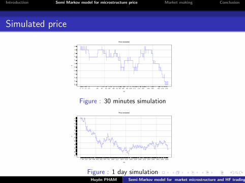
Simulated price

Price simulation

t(s)

P

0 47 111 176 349 447 533 599 688 755 818 886 968 1039 1121 1215 1295 1406 1493 1623 1700 1785

−10

−9

−8

−7

−6

−5

−4

−3

−2

−1

01

Figure : 30 minutes simulation

Price simulation

t(s)

P

0 804 1919 3148 4384 5623 6851 8079 9311 10650 12117 13670 15129 16650 18105 19558 21010 22463 23943 25491 26951 28424

−62

−56

−50

−44

−38

−32

−26

−20

−14

−9

−4

0

Figure : 1 day simulationHuyen PHAM Semi-Markov model for market microstructure and HF trading


Diffusive behavior at macroscopic scale

Scaling:

P(T )t =

PtT√T, t ∈ [0, 1].

Theorem

limT→∞

P(T ) (d)= σ∞W ,

where W is a Brownian motion, and σ2∞ is the macroscopicvariance:

σ2∞ = λ(1 + α

1− α

).

with λ−1 =∫∞0 tdF (t).



Mean signature plot (realized volatility)

We consider the case of delayed renewal process:

Sn ; F , n ≥ 1, with finite mean 1/λ, and S1 ; density λ(1− F )

→ Price process P has stationary increments

Proposition

V (τ) :=1

τE[(Pτ − P0)2] = σ2∞ +

( −2α

1− α

)1− Gα(τ)

(1− α)τ,

where Gα(t) = E[αNt ] is explicitly given via its Laplace-Stieltjestransform Gα in terms of F (s) :=

∫∞0− e−stdF (t).

V (∞) = σ2∞ , and V (0+) = λ.

Remark: Similar expression as in Robert and Rosenbaum (09) orBacry et al. (11).



0 500 1000 1500 2000 2500 3000 3500

0.00

050.

0010

0.00

150.

0020

0.00

25

Signature Plot

tau(s)

C(t

au)

DataSimulationGammaPoisson

Figure : Mean signature plot for α < 0



Markov embedding of price process

• Define the the last price jump direction:

It = JNt , t ≥ 0, valued in {+1,−1}

and the elapsed time since the last jump:

St = t − supTk≤t

Tk , t ≥ 0.

I Then the price process (Pt) valued in 2δZ is embedded in a Markovprocess with three observable state variables (Pt , It ,St) with generator:

Lϕ(p, i , s) =∂ϕ

∂s+ h+(s)

[ϕ(p + 2δi , i , 0)− ϕ(p, i , s)

]+ h−(s)

[ϕ(p − 2δi ,−i , 0)− ϕ(p, i , s)

],



Trading issue

Problem of an agent (market maker) who submits limit orders onboth sides of the LOB: limit buy order at the best bid price andlimit sell order at the best ask price, with the aim to gain thespread.

I We need to model the market order flow, i.e. the counterparttrade of the limit order



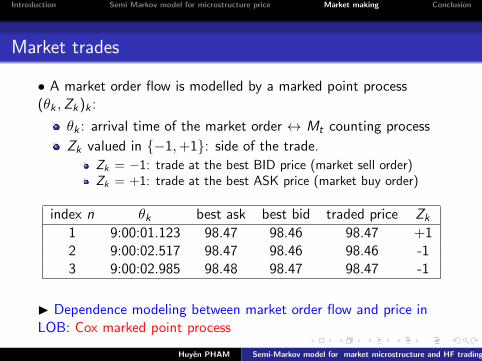
Market trades

• A market order flow is modelled by a marked point process(θk ,Zk)k :

θk : arrival time of the market order ↔ Mt counting process

Zk valued in {−1,+1}: side of the trade.

Zk = −1: trade at the best BID price (market sell order)Zk = +1: trade at the best ASK price (market buy order)

index n θk best ask best bid traded price Zk

1 9:00:01.123 98.47 98.46 98.47 +12 9:00:02.517 98.47 98.46 98.46 -13 9:00:02.985 98.48 98.47 98.47 -1

I Dependence modeling between market order flow and price inLOB: Cox marked point process



Trade timestamp modeling

• The counting process (Mt) of the market order timestamps (θk)kis a Cox process with conditional intensity λ

M(St).

Examples of parametric forms reproducing intensity decay when sis large:

λexpM (s) = λ0 + λ1sre−ks

λpowerM (s) = λ0 +λ1s

r

1 + sk.

with positive parameters λ0, λ1, r , k , estimated by MLE.



Strong and weak side of LOB

First level limit orders

BEST ASK PRX

BEST BID PRX


Second level limit orders

BEST ASK PRX

BEST BID PRX




BEST ASK PRX

BEST BID PRX




• We call strong side (+) of the LOB, the side in the samedirection than the last jump, e.g. best ask when price jumpedupwards.

• We call weak side (−) of the LOB, the side in the oppositedirection than the last jump, e.g. best bid when price jumpedupwards.

I We observe that trades (market order) arrive mostly on theweak side of the LOB.



Trade side modeling

• The trade sides are given by:

Zk = Γk Iθ−k,

(Γk)k i.i.d. valued in {+1,−1} with law:

P[Γk = ±1] =1± ρ

2

for ρ ∈ [−1, 1].



Interpretation of ρ

ρ = corr(Zk , Iθ−k)

ρ = 0: market order flow arrive independently at best bid andbest ask (usual assumption in the existing literature)

ρ > 0: market orders arrive more often in the strong side ofthe LOB

ρ < 0: market orders arrive more often in the weak side of theLOB

• Estimation of ρ: ρn = 1n

∑nk=1 Zk Iθ−k

leads to ρ ' −50%: about

3 over 4 trades arrive on the weak side.I ρ related to adverse selection



Market making strategy

• Strategy control: predictable process (`+t , `−t )t valued in {0, 1}

`+t = 1: limit order of fixed size L on the strong side: +It−

`−t = 1: limit order of fixed size L on the weak side: −It−

• Fees: any transaction is subject to a fixed cost ε ≥ 0

I Portfolio process:

Cash (Xt)t valued in R,

inventory (Yt)t valued in a set Y of Z



Agent execution

• Execution of limit order occurs when:

A market trade arrives at θk on the strong (resp. weak) sideif Zk Iθ−k

= +1 (resp. −1), and with an executed quantity

given by a distribution (price time priority/prorata) ϑ+L (resp.ϑ−L ) on {0, . . . , L}The price jumps at Tk and crosses the limit order price

Remarkϑ±L cannot be estimated on historical data. It has to be evaluatedby a backtest with a zero intelligence strategy.

I Risks:

Inventory ↔ price jump

Adverse selection in market order trade



Market making optimization

• Value function of the market making control problem:

v(t, s, p, i , x , y) = sup(`+,`−)

E[PNLT − CLOSE (YT )− η · RISKt,T

]where η ≥ 0 is the agent risk aversion and:

PNLt = Xt + Yt · Pt , (ptf valued at the mid price)

CLOSE (y) = −(δ + ε) · |y |, (closure market order)

RISKt,T =

∫ T

tY 2u · d [P]u, (no inventory imbalance)



Variable reduction to strong inventory and elapsed time

Theorem

The value function is given by:

v(t, s, p, i , x , y) = x + yp + ωyi (t, s)

where ωq(t, s) = ω(t, s, q) is the unique viscosity solution to theintegro ODE:[∂t + ∂s

]ω + 2δ(h+ − h−)q − 4δ2η(h+ + h−)q2

+ max`∈{0,1},q−`L∈Y

L`+ ω + max`∈{0,1},q+`L∈Y

L`− ω = 0

ωq(T , s) = −|q| (δ + ε)

in [0,T ]× R+ × Y.



L`± = L`±,M

+ L`±,jump

favorable execution of random size ≤ L by market order

L`±,M

ω := λ±,M(s)

∫ [ω(t, s, q ∓ k`)− ω(t, s, q)

+ (+δ − ε)k`]ϑ±L (dk)

unfavorable execution of maximal size L due to price jump

L`±,jumpω := h±(s)

[ω(t, 0,±q − L`)− ω(t, s, q) + (−δ − ε)L`

]with

λ±,M(s) :=

1± ρ2· λ

M(s) (trade intensities)



Optimal policy shape: ρ = 0, execution probability = 10%



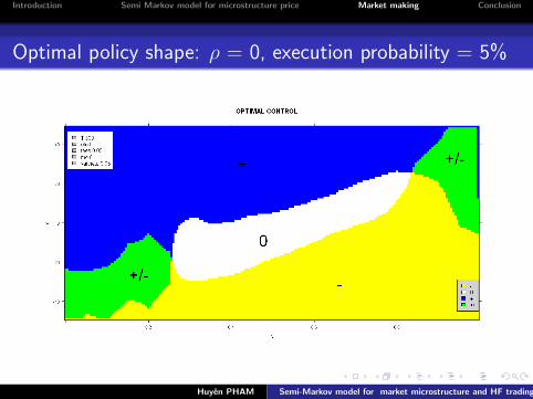
Optimal policy shape: ρ = 0, execution probability = 5%



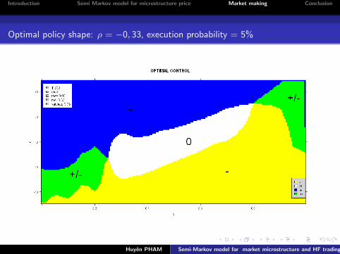
Optimal policy shape: ρ = −0, 33, execution probability = 5%



Concluding remarks

• Markov renewal approach for market microstructure

+ Easy to understand and simulate

+ Non parametric estimation based on i.i.d. sample data

+ dependency between price return Jk and jump time Tk

+ Reproduces well microstructure effects, diffuses onmacroscopic scale

+ Markov embedding with observable state variables ( 6= Hawkesprocess approach)

+ Develop stochastic control algorithm for HF trading

- MRP forgets correlation between inter-arrival jump times {Sk= Tk − Tk−1}k

• Extension to multivariate price model

• Model with market impact for liquidation problemHuyen PHAM Semi-Markov model for market microstructure and HF trading

semi-markov model for market microstructure and hf...

Documents