semi-analytical treatment of complex nonlinear

Available online at www.worldscientificnews.com

( Received 20 January 2020; Accepted 09 February 2020; Date of Publication 10 February 2020 )

WSN 142 (2020) 1-24 EISSN 2392-2192

Semi-analytical treatment of complex nonlinear oscillations arising in the slider-crank mechanism

Akuro Big-Alabo*, Collins Onyinyechukwu Ogbodo and Chinwuba Victor Ossia

Applied Mechanics & Design (AMD) Research Group, Department of Mechanical Engineering, Faculty of Engineering, University of Port Harcourt, Port Harcourt, Nigeria

*E-mail address: [email protected]

ABSTRACT

The model for the free nonlinear oscillation of the slider-crank mechanism is very complicated

and difficult to solve accurately using most of the existing approximate analytical schemes. However,

the continuous piecewise linearization method (CPLM), which is a recently proposed semi-analytical

algorithm, is capable of producing simple and accurate periodic solutions for conservative systems

irrespective of the complexity of the nonlinear restoring force. Hence, this study applied the CPLM to

solve and analyze the complex nonlinear oscillations arising in the slider-crank mechanism. The CPLM

results were verified using numerical solutions and it was found that the CPLM solution was accurate

to less than 1.0% for angular amplitudes up to 165°. Analysis of the frequency-amplitude response

revealed the existence of asymptotic behaviour as the ratio of the crank radius to the connecting rod

length approaches zero or unity. Hence, oscillation models for the observed asymptotic responses were

derived and found to be significantly simpler compared to the original oscillation model. Finally,

analysis of the large-amplitude oscillations of the slider-crank mechanism revealed the presence of

strong anharmonic response.

Keywords: Slider-crank mechanism, nonlinear oscillation, conservative system, non-natural system,

continuous piecewise linearization method, periodic solution

http://www.worldscientificnews.com/

World Scientific News 142 (2020) 1-24

-2-

1. INTRODUCTION

Nonlinear oscillation of structures and systems is of interest to engineers, natural

scientists, and mathematicians. Knowledge of the periodic response of a nonlinear oscillator is

important for understanding the system’s behaviour and is necessary for design purposes. The

dynamic models of most oscillators are in the form of nonlinear ordinary differential equations,

the exact solutions of which are not available in many cases. Therefore, numerical or

approximate analytical solutions are usually applied to derive the periodic response of most

nonlinear oscillators.

In recent times, approximate analytical solutions have become attractive and many such

methods have been developed to determine the periodic response of various nonlinear systems

such as Duffing oscillator [1], simple pendulum [2], pendulum with rotating support [3], mass

attached to the mid-point of an inextensible string [4, 5], geometrically nonlinear crank [6],

two-mass system [7-9], vibration of cracked plate [10, 11], beams [12], relativistic simple

harmonic oscillator [13, 14], micro- and nano-electromechanical devices [15, 16], oscillator

with coordinate-dependent mass [17] and fractal systems [18]. Most of the existing approximate

analytical methods for solving nonlinear oscillators [4, 5, 19-30] are either algebraically

intractable or inaccurate when applied to solve oscillators with complex nonlinearity. The

continuous piecewise linearization method (CPLM) is a simple and accurate algorithm that was

formulated to solve models of nonlinear conservative oscillators notwithstanding the

complexity of the nonlinear restoring force [1, 31].

The slider-crank mechanism is a classic mechanical system whose dynamic response has

been investigated by many [32-40]. The slider-crank mechanism with a rigid connecting rod

exhibits complex nonlinear vibrations and the oscillation model has been discussed in the

literature [35, 41]. However, due to the complex nature of the oscillation model, only numerical

solutions to the oscillation model have been presented [35].

To explore the potential of the CPLM to accurately predict complex nonlinear oscillations

of physical systems, we apply the CPLM to investigate the periodic response of the slider-crank

oscillations. In order to achieve this, the conventional form of the slider-crank oscillation model

was first transformed into a conservative form that shows the nonlinear restoring force

explicitly.

The CPLM algorithm was then applied to the conservative form of the model to derive

frequency-amplitude responses and oscillation histories that were used to analyse the small-

amplitude and large-amplitude oscillations. The CPLM results were verified by comparing with

accurate numerical results.

2. MATHEMATICAL MODEL

2. 1. Description of slider-crank mechanism

The slider-crank mechanism is a well-known mechanical system that can be used to

convert rotary motion to translational motion and vice versa. The slider-crank mechanism is a

special case of the four-bar linkage mechanism [32].

It has a crank, which rotates about its supported end, and a connecting rod, which connects

the crank to the slider mass. An illustration of the slider-crank mechanism is shown in Figure

1.


-3-

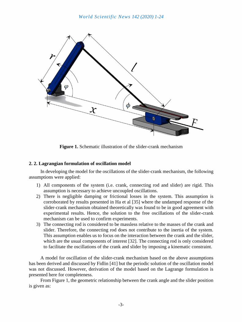
Figure 1. Schematic illustration of the slider-crank mechanism

2. 2. Lagrangian formulation of oscillation model

In developing the model for the oscillations of the slider-crank mechanism, the following

assumptions were applied:

1) All components of the system (i.e. crank, connecting rod and slider) are rigid. This

assumption is necessary to achieve uncoupled oscillations.

2) There is negligible damping or frictional losses in the system. This assumption is

corroborated by results presented in Ha et al [35] where the undamped response of the

slider-crank mechanism obtained theoretically was found to be in good agreement with

experimental results. Hence, the solution to the free oscillations of the slider-crank

mechanism can be used to confirm experiments.

3) The connecting rod is considered to be massless relative to the masses of the crank and

slider. Therefore, the connecting rod does not contribute to the inertia of the system.

This assumption enables us to focus on the interaction between the crank and the slider,

which are the usual components of interest [32]. The connecting rod is only considered

to facilitate the oscillations of the crank and slider by imposing a kinematic constraint.

A model for oscillation of the slider-crank mechanism based on the above assumptions

has been derived and discussed by Fidlin [41] but the periodic solution of the oscillation model

was not discussed. However, derivation of the model based on the Lagrange formulation is

presented here for completeness.

From Figure 1, the geometric relationship between the crank angle and the slider position

is given as:


-4-

𝑥 = 𝑟 cos𝜑 + 𝑙√1 − Ω2 sin2 𝜑 (1𝑎)

where 𝑥 is the slider position measured from the centre of rotation of the crank and Ω = 𝑟/𝑙 is

a dimensionless geometric constant.

The velocity of the slider can be derived by differentiating equation (1a) as shown:

= 𝑑𝑥

𝑑𝜑= −𝑟

(

sin𝜑 +Ω sin 2𝜑

2√1 − Ω2 sin2 𝜑)

(1b)

Since the connecting rod is assumed to be massless, the kinetic energy is given as:

𝑇 =1

2𝑀𝑐𝑟

22 +1

2𝑀𝑠

2 (2a)

Therefore,

𝑇 =1

2𝑀𝑐𝑟

22 +1

2𝑀𝑠𝑟

2

(


2√1 − Ω2 sin2𝜑)

2

2 =1

2𝐽(𝜑)2 (2b)

where 𝐽(𝜑) is the effective moment of inertia given as:

𝐽(𝜑) = 𝑀𝑐𝑟2 +𝑀𝑠𝑟

2

(


2√1 − Ω2 sin2𝜑)

2

(3)

We note that the velocity squared in equation (2b) is multiplied by a displacement-

dependent inertia, 𝐽(𝜑), which means that the kinetic energy is not a pure quadratic function of

velocity. This quality is characteristic of non-natural oscillators [31, 42].

The potential energy of the connecting rod is negligible since it is massless. Also, the

crank and the slider have no potential energies. Hence, the total potential energy of the system

is 𝑉 = 0.

Therefore, the Lagrangian is:

𝐿 = 𝑇 − 𝑉 =1

2𝐽(𝜑)2 (4)

Now, the oscillation model can be derived from the Lagrange equation given as:

𝑑

𝑑𝑡(𝜕𝐿

𝜕) −

𝜕𝐿

𝜕𝜑= 𝑄 (5)


-5-

Substituting equation (4) in (5) we get:

𝐽(𝜑) +1

2𝐽′(𝜑)2 − 𝑄(𝜑) = 0 (6)

The initial conditions to equation (6) are 𝜑(0) = 𝜑0 and (0) = 0, and the prime denotes

differentiation with respect to 𝜑. Also, 𝑄(𝜑) is the generalized force given as:

𝑄(𝜑) = 𝐹𝜕𝑥

𝜕𝜑= −𝐹𝑟

(


2√1 − Ω2 sin2 𝜑)

(7)

where 𝐹 > 0. Differentiating equation (3), we get:

𝐽′(𝜑) = 𝑀𝑠𝑟2 (sin 2𝜑 + (

Ω

𝑐) (cos𝜑 sin 2𝜑 + 2 cos 2𝜑 sin𝜑) +

1

2(Ω

𝑐)2

sin 4𝜑

+1

2(Ω

𝑐)3

sin2 2𝜑 sin𝜑 +1

4(Ω

𝑐)4

sin3 2𝜑) (8)

where 𝑐 = √1 − Ω2 sin2 𝜑. At this point, if we substitute equations (3), (7) and (8) in equation

(6), we arrive at the nonlinear model governing the periodic response of the crank as shown in

equation (9).

[𝑀𝑐𝑟2 +𝑀𝑠𝑟

2 (sin 𝜑 +1

2(Ω

𝑐) sin 2𝜑)

2

] +1

2𝑀𝑠𝑟

2

[sin 2𝜑 + (Ω


1

2(Ω

𝑐)2

sin 4𝜑 +1

2(Ω

𝑐)3

sin2 2𝜑 sin 𝜑

+1

4(Ω

𝑐)4

sin3 2𝜑] 2 + 𝐹𝑟 (sin𝜑 +1

2(Ω

𝑐) sin 2𝜑) = 0 (9)

Equation (9) is a very complicated nonlinear oscillator and the main challenge lies in

deriving an accurate periodic solution for this oscillator using approximate analytical schemes.

This paper addresses this challenge by applying the CPLM algorithm to derive accurate periodic

solutions. This way, the potential of the CPLM algorithm to handle complex nonlinear

oscillators is being explored and confirmed.

2. 3. Conservative form of oscillation model

Equation (6) governs the motion of a conservative system but it is not in the standard

conservative form that contains an explicit expression for the restoring force. However, the

conservative form can be derived as follows.

Assuming = 𝑦, then equation (6) can be written as:


-6-

𝐽(𝜑)𝑦𝑑𝑦 + (1

2𝐽′(𝜑)𝑦2 − 𝑄(𝜑))𝑑𝜑 = 0 (10)

Equation (10) is an exact differential equation and its solution is:

𝐸(𝜑, ) =1

2𝐽(𝜑)2 + ℎ(𝜑) = ℎ(𝜑0) (11)

where ℎ(𝜑) = −∫𝑄(𝜑)𝑑𝜑 = −𝐹𝑟(cos𝜑 + Ω√1 − Ω2 sin2𝜑 ) and ℎ(𝜑0) is a constant

representing the total energy in the slider-crank mechanism. Equation (11) is a mathematical

statement of the conservation of energy for equation (6) and it confirms that the Hamiltonian

function, 𝐻 = 𝑇 + 𝑉 =1

2𝐽(𝜑)2, is not constant. Hence, the slider-crank mechanism may be

referred to as a non-Hamiltonian conservative system because it does not admit a constant

Hamiltonian function [31].

From equation (11) the state-space relationship is:

2 =2[ℎ(𝜑0) − ℎ(𝜑)]

𝐽(𝜑) (12)

Substituting equation (12) in (6) and simplifying gives:

+𝐽′(𝜑)[ℎ(𝜑0) − ℎ(𝜑)]

[𝐽(𝜑)]2−𝑄(𝜑)

𝐽(𝜑)= 0 (13)

Equation (13) represents the conservative form of equation (6) and can be expressed as:

+ 𝑔(𝜑) = 0 (14)

where 𝑔(𝜑) is the restoring force given as:

𝑔(𝜑) =𝐽′(𝜑)[ℎ(𝜑0) − ℎ(𝜑)]

[𝐽(𝜑)]2−𝑄(𝜑)

𝐽(𝜑)

Carrying out the necessary substitutions and after algebraic simplification, the restoring

force for the oscillation of the crank can be expressed as:


-7-

𝑔(𝜑) =𝐹𝑀𝑠𝑟

3[cos𝜑 − cos𝜑0 + Ω(𝑐 − √1 − Ω2 sin2𝜑0 )]

[𝑀𝑐𝑟2 +𝑀𝑠𝑟2 (sin𝜑 +12 (Ω𝑐) sin 2𝜑)

2

]

2 (sin 2𝜑

+ (Ω


1

2(Ω

𝑐)2

sin 4𝜑

+1

2(Ω

𝑐)3

sin2 2𝜑 sin𝜑 +1

4(Ω

𝑐)4

sin3 2𝜑)

+𝐹𝑟 (sin 𝜑 +

12 (Ω𝑐) sin 2𝜑)

𝑀𝑐𝑟2 +𝑀𝑠𝑟2 (sin𝜑 +12 (Ω𝑐) sin 2𝜑)

2 (15)

A typical plot of equation (15) when 𝜑0 = 𝜋 is shown in Figure 2, and the plot reveals

the highly nonlinear nature of the crank oscillation for large initial amplitudes. Figure 3 shows

a plot of the phase diagram for the crank oscillation and it reveals the existence of periodic

oscillations around the origin, for all feasible amplitudes i.e. 0 < 𝜑0 < 𝜋.

The corresponding phase diagram for the slider oscillation is shown in Figure 4.

The latter reveals that the centre of periodic oscillation for the slider depends on the initial

amplitude of the crank.

Figure 2. Restoring force for the crank oscillation when 𝜑0 = 𝜋 rad.

-30

-20

-10

0

10

20

30

-4 -3 -2 -1 0 1 2 3 4

Re

sto

rin

g f

orc

e (

N/k

gm

2)

Crank displacement (rad)


-8-

Figure 3. Phase diagram for the crank oscillation when 𝜑0 = 𝜋/6, 𝜋/3, 𝜋/2, 2𝜋/3, 5𝜋/6, and

𝜋 rad. The oscillation amplitude was increased each time by 𝜋/6 from the innermost to the

outermost plot.

Figure 4. Phase diagram for the slider oscillation when 𝜑0 = 𝜋/6, 𝜋/3, 𝜋/2, 2𝜋/3, 5𝜋/6, and

𝜋 rad. The oscillation amplitude was increased each time by 𝜋/6 from the innermost to the

outermost plot.

-10

-8

-6

-4

-2

0

2

4

6

8

10

-4 -3 -2 -1 0 1 2 3 4

Cra

nk

ve

loci

ty (

rad

/s)

Crank displacement (rad)

ϕ0 = π

ϕ0 = π/6

-0.8

-0.6

-0.4

-0.2

0

0.2

0.4

0.6

0.8

0.35 0.4 0.45 0.5 0.55 0.6 0.65

Slid

er

velo

city

(m

/s)

Slider displacement (m)

ϕ0 = π/6

ϕ0 = π


-9-

3. APPROXIMATE PERIODIC SOLUTION

The conservative form of the nonlinear oscillation model for the crank (i.e. equations (14)

and (15)) was solved using the CPLM algorithm. The algorithm is based on the piecewise

discretization and linearization of the nonlinear restoring force. In order to be concise, details

on the concept and formulation of the CPLM algorithm are not discussed here and the interested

reader can refer to the following articles [1, 31]. Here, the main results of the CPLM solution

for nonlinear conservative models are presented.

According to the CPLM algorithm [1], the linearized stiffness for each discretization of

the nonlinear restoring force 𝑔(𝜑) can be written as 𝐾𝑝𝑞 = [𝑔(𝜑𝑞) − 𝑔(𝜑𝑝)]/(𝜑𝑞 − 𝜑𝑝). Consequently, the CPLM solution for the displacement and time interval covered by each

discretization depends on whether 𝐾𝑝𝑞 is positive or negative [31].

3. 1. Solution for positive linearized stiffness

If 𝐾𝑝𝑠 > 0, then the displacement for each discretization can be expressed as:

𝜑(𝑡) = 𝑅𝑝𝑞 sin(𝜔𝑝𝑞𝑡 + Φ𝑝𝑞) + 𝐶𝑝𝑞 (16)

where 𝑅𝑝𝑞 = [(𝜑𝑝 − 𝐶𝑝𝑞)2+ (𝑝/𝜔𝑝𝑞)

2]1/2

, 𝜔𝑝𝑞 = √𝐾𝑝𝑞 and 𝐶𝑝𝑞 = 𝜑𝑝 − 𝑔(𝜑𝑝)/𝐾𝑝𝑞. The

initial conditions (𝜑𝑝, 𝑝) and other parameters (Φ𝑝𝑞, ∆𝑡) are determined based on the

oscillation stage. For the oscillation stage that moves from +𝜑0 to −𝜑0 the initial conditions

for each discretization are 𝜑𝑝 = 𝜑𝑝(0) = 𝜑0 − 𝑝∆𝜑 and 𝑝 = 𝑝(0) =

−√|2∫ −𝑔(𝜑)𝑑𝜑𝜑𝑝

𝜑0|; where ∆𝜑 = 𝜑0/𝑛 and the other parameters are calculated as:

Φ𝑝𝑠 = 0.5𝜋 𝑝 = 0

𝜋 + tan−1[𝜔𝑝𝑞(𝜑𝑝 − 𝐶𝑝𝑞)/𝑝] 𝑝 < 0 (17a)

∆𝑡 = (0.5𝜋 − Φ𝑝𝑞)/𝜔𝑝𝑞 (𝜑𝑞 − 𝐶𝑝𝑞) ≥ 𝑅𝑝𝑞

(0.5𝜋 + cos−1[(𝜑𝑞 − 𝐶𝑝𝑞)/𝑅𝑝𝑞] − Φ𝑝𝑞)/𝜔𝑝𝑞 (𝜑𝑞 − 𝐶𝑝𝑞) < 𝑅𝑝𝑞 (17b)

For the oscillation stage that moves from −𝜑0 to +𝜑0 the initial conditions are

𝜑𝑝 = 𝜑𝑝(0) = −𝜑0 + 𝑝∆𝜑 and 𝑝 = 𝑝(0) = √|2 ∫ −𝑔(𝜑)𝑑𝜑𝜑𝑝

𝜑0| ; the other parameters are

calculated as:

Φ𝑝𝑠 = −0.5𝜋 𝑝 = 0

tan−1[𝜔𝑝𝑠(𝜑𝑝 − 𝐶𝑝𝑠)/𝑝] 𝑝 < 0 (18a)

∆𝑡 = (0.5𝜋 − Φ𝑝𝑞)/𝜔𝑝𝑞 (𝜑𝑞 − 𝐶𝑝𝑞) ≥ 𝑅𝑝𝑞

(0.5𝜋 + cos−1[(𝜑𝑞 − 𝐶𝑝𝑞)/𝑅𝑝𝑞] − Φ𝑝𝑞)/𝜔𝑝𝑞 (𝜑𝑞 − 𝐶𝑝𝑞) < 𝑅𝑝𝑞 (18b)


-10-

At the end of each discretization, 𝑡𝑞 = 𝑡𝑝 + ∆𝑡 and the end variables (𝜑𝑞 and 𝑞) are

determined by replacing 𝑝 with 𝑞 in the formulae for the initial conditions.

3. 2. Solution for negative linearized stiffness

If 𝐾𝑝𝑞 < 0, then the solution of the displacement for each discretization is:

𝜑(𝑡) = 𝐴𝑟𝑠𝑒𝜔𝑝𝑞𝑡 + 𝐵𝑟𝑠𝑒

−𝜔𝑝𝑞𝑡 + 𝐶𝑝𝑞 (19)

where 𝜔𝑝𝑞 = √|𝐾𝑝𝑞|, 𝐶𝑝𝑞 = 𝜑𝑝 + 𝑔(𝜑𝑝)/|𝐾𝑝𝑞| and 𝐴𝑝𝑞 and 𝐵𝑝𝑞 are integration constants that

depend on the initial conditions. Therefore, 𝐴𝑝𝑞 =1

2(𝜑𝑝 − 𝐶𝑝𝑞 + 𝑝/𝜔𝑝𝑞) and

𝐵𝑝𝑞 =1

2(𝜑𝑟 − 𝐶𝑝𝑞 − 𝑝/𝜔𝑝𝑞). The initial and end conditions are computed in the same way

as in the case of 𝐾𝑝𝑞 > 0. Applying the end conditions in equation (5) gives the time interval

for each discretization as:

∆𝑡 =

1

𝜔𝑝𝑞log𝑒

[ (𝜑𝑞 − 𝐶𝑝𝑞) ± √(𝜑𝑞 − 𝐶𝑝𝑞)

2− 4𝐴𝑝𝑞𝐵𝑝𝑞

2𝐴𝑝𝑞

]

(𝜑𝑞 − 𝐶𝑝𝑞) > 2√𝐴𝑝𝑞𝐵𝑝𝑞

1

𝜔𝑝𝑞log𝑒 (

𝜑𝑞 − 𝐶𝑝𝑞

2𝐴𝑝𝑞 ) (𝜑𝑞 − 𝐶𝑝𝑞) ≤ 2√𝐴𝑝𝑞𝐵𝑝𝑞

(20)

The sign before the square root in equation (20a) is negative for the oscillation stage that

moves from −𝜑0 to +𝜑0 and vice versa.

In rare occasions there may be a possibility of having 𝐾𝑝𝑞 = 0 for one or two

discretizations and this would result in a computational error. This scenario occurs around the

turning points or relatively flat regions of the restoring force and is likely when 𝑛 is very large.

When this happens, it can be eliminated by increasing or decreasing 𝑛 slightly.

4. RESULTS AND DISCUSSIONS

In order to investigate the periodic response of the slider-crank mechanism in Figure 1,

the following inputs were used except where it is otherwise stated: 𝑟 = 0.10𝑚; 𝑙 = 0.50𝑚;

𝑀𝑐 = 0.50𝑘𝑔; 𝑀𝑠 = 0.30𝑘𝑔; 𝐹 = 1.0𝑁. These input values were also used to simulate the

plots in Figures 2 to 4 above.

The CPLM algorithm explained in Section 3 was implemented by means of a simple

Mathematica code that was used to simulate the periodic response of the slider-crank

oscillations. The CPLM parameters that were determined from the restoring force are: 𝐾𝑝𝑞 =

[𝑔(𝜑𝑞) − 𝑔(𝜑𝑝)]/(𝜑𝑞 − 𝜑𝑝), 𝐶𝑝𝑞 = 𝜑𝑝 − 𝑔(𝜑𝑝)/𝐾𝑝𝑞 and 𝑝 = ±√|2∫ −𝑔(𝜑)𝑑𝜑𝜑𝑝

𝜑0|.

We note that 𝐾𝑝𝑞 and 𝐶𝑝𝑞 can be easily calculated from equation (15) while the expression

to calculate 𝑟 was derived from equation (12) as:


-11-

𝑝 = ±√2𝐹𝑟[cos𝜑𝑝 − cos𝜑0 + Ω(√1 − Ω2 sin2 𝜑𝑝 −√1 − Ω2 sin2𝜑0 )]

𝑀𝑐𝑟2 +𝑀𝑠𝑟2 (sin𝜑𝑝 +12 (𝛺𝑐) sin 2𝜑𝑝)

2 (21)

The remaining parameters of the CPLM algorithm depend on these three parameters and

the discretization process. The CPLM algorithm for equations (14) and (15) has been

summarized in the pseudocode algorithm provided in the appendix.

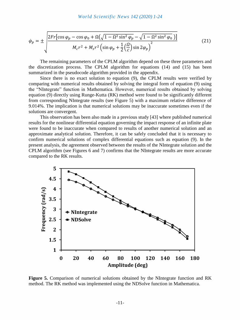
Since there is no exact solution to equation (9), the CPLM results were verified by

comparing with numerical results obtained by solving the integral form of equation (9) using

the “NIntegrate” function in Mathematica. However, numerical results obtained by solving

equation (9) directly using Runge-Kutta (RK) method were found to be significantly different

from corresponding NIntegrate results (see Figure 5) with a maximum relative difference of

9.014%. The implication is that numerical solutions may be inaccurate sometimes even if the

solutions are convergent.

This observation has been also made in a previous study [43] where published numerical

results for the nonlinear differential equation governing the impact response of an infinite plate

were found to be inaccurate when compared to results of another numerical solution and an

approximate analytical solution. Therefore, it can be safely concluded that it is necessary to

confirm numerical solutions of complex differential equations such as equation (9). In the

present analysis, the agreement observed between the results of the NIntegrate solution and the

CPLM algorithm (see Figures 6 and 7) confirms that the NIntegrate results are more accurate

compared to the RK results.

Figure 5. Comparison of numerical solutions obtained by the NIntegrate function and RK

method. The RK method was implemented using the NDSolve function in Mathematica.

1

1.5

2

2.5

3

3.5

4

4.5

5

0 20 40 60 80 100 120 140 160 180

Fre

qu

en

cy (

rad

/s)

Amplitude (deg)

NIntegrate

NDSolve


-12-

Figure 6. Frequency-amplitude response of the crank oscillation for 10° ≤ 𝜑0 ≤ 170°.

Figure 7. Error analysis in CPLM solution for the frequency-amplitude response of

the crank oscillation.

1.6

2

2.4

2.8

3.2

3.6

4

4.4

4.8

0 20 40 60 80 100 120 140 160 180

Fre

qu

en

cy (

rad

/s)

Amplitude (deg)

Numerical

CPLM ( n = 25 )

CPLM ( n = 50 )

CPLM ( n = 100 )

CPLM ( n = 200 )

0

0.5

1

1.5

2

2.5

3

3.5

0 20 40 60 80 100 120 140 160 180

Re

lati

ve d

iffe

ren

ce (

%)

Amplitude (deg)

CPLM ( n = 25 )

CPLM ( n = 50 )

CPLM ( n = 100 )

CPLM ( n = 200 )


-13-

4. 1. Frequency-amplitude response

The frequency-amplitude response for initial amplitudes in the range of 10° ≤ 𝜑0 ≤170° is shown in Figure 6. The figure shows both CPLM and NIntegrate results. The CPLM

results are seen to converge as 𝑛 increases from 25 to 200. The corresponding relative

percentage differences (RPDs) between the CPLM results and the NIntegrate results are shown

in Figure 7.

The maximum RPD for 𝑛 = 25 is 3.297%, 𝑛 = 50 is 2.186%, 𝑛 = 100 is 1.479% and

for 𝑛 = 200 is 1.018%. Furthermore, the CPLM frequency for 𝑛 = 200 when 𝜑0 = 179° is

1.10978 rad/s with an RPD of 2.53432%. These RPDs are well within acceptable limits in

engineering practice. However, more accurate results can be obtained by using 𝑛 > 200.

Figure 6 also reveals that the frequency decreases steadily with an increase in amplitude.

Since the time period of the crank is twice that of the slider, it implies that the frequency

response of the slider is twice that of the crank and has the same trend as in Figure 6.

4. 2. Effect of geometric constant on frequency response

To ensure that the slider does not lift off the floor the following constraint is imposed:

𝑥0/(𝑟 + 𝑙) ≥ 𝑘, where 0 < 𝑘 < 1 and 𝑥0 is the slider position at maximum crank angle, 𝜑0.

For the limit, 𝑘 = 0, the condition of 𝑥0 = 0 represents a case in which the initial slider position

coincides with the crank centre and it implies that 𝜑0 = 90° while 𝑟 = 𝑙. On the other hand,

when 𝑘 = 1 the condition of 𝑥0 = 𝑟 + 𝑙 represents a situation where there is no oscillation

because 𝜑0 = 0°. However, the condition of 𝑥0 > 𝑟 + 𝑙 is impossible by virtue of the kinematic

constraint.

Substituting equation (1a) in the ‘no-lift’ constraint gives:

Ω cos𝜑0 +√1 − Ω2 sin2𝜑0 ≥ 𝑘(Ω + 1) (22)

The solution to equation (22) provides the range of values of the geometric constant (see

equation (23)) for which the slider does not lift off the floor.

Ω ≤1 − 𝑘2

1 + 𝑘2 − 2𝑘 cos𝜑0 (23)

Equation (23) can be used for design purposes and we can deduce from this equation that Ω ≤(1 − 𝑘2)/(1 + 𝑘2) < 1 for all 𝑘 when 𝜑0 = 90°, whereas Ω ≤ 1 for all possible values of 𝜑0

when 𝑘 = 0.

To simulate the effect of the geometric constant on the frequency response, 𝑘 = 0.1 was

assumed. This means that the distance from the slider position to the crank centre cannot be

less than 0.1 × (𝑟 + 𝑙). Therefore, when 𝜑0 = 60°, Ω ≤ 1.0879 and when 𝜑0 = 120°, Ω ≤0.8919. Figures 8 and 9 show the variation of the frequency with Ω for different crank radii

when 𝜑0 = 60° and 120° respectively. In these figures and subsequent ones, the CPLM results

are plotted as solid lines while the numerical integration results are plotted as circle markers.

The results show that for the same value of Ω the frequency decreases with an increase in

crank radius. In addition, Figures 8 and 9 reveal the existence of asymptotic behaviour as Ω →0 and Ω → 1.0.


-14-

Figure 8. Effect of geometric constant on frequency response

for various crank radii when 𝜑0 = 60°.

Figure 9. Effect of geometric constant on frequency response

for various crank radii when 𝜑0 = 120°.

0

0.5

1

1.5

2

2.5

3

3.5

4

4.5

0 0.2 0.4 0.6 0.8 1

Fre

qu

en

cy (

rad

/s)

Ω

r = 0.1 r = 0.2r = 0.3

r = 0.4 r = 0.5

0

0.5

1

1.5

2

2.5

3

0 0.1 0.2 0.3 0.4 0.5 0.6 0.7 0.8

Fre

qu

en

cy (

rad

/s)

Ω

r = 0.1 r = 0.2r = 0.3

r = 0.4 r = 0.5


-15-

4. 3. Asymptotic models

Figures 8 and 9 revealed the presence of asymptotic response under two limiting

geometric conditions and the oscillation models for the asymptotic responses can be derived as

follows.

Case 1: Ω → 0

Applying this condition in equations (3) and (7) gives the following: 𝐽(𝜑) = 𝑀𝑐𝑟2 +

𝑀𝑠𝑟2 sin2 𝜑, 𝐽′(𝜑) = 𝑀𝑠𝑟

2 sin 2𝜑 and 𝑄(𝜑) = −𝐹𝑟 sin𝜑. Therefore, substituting these

expressions in equation (6), the oscillation model of the crank was derived as equation (24).

(𝑀𝑐𝑟2 +𝑀𝑠𝑟

2 sin2𝜑) +1

2𝑀𝑠𝑟

2 sin 2𝜑 2 + 𝐹𝑟 sin𝜑 = 0 (24)

Furthermore, ℎ(𝜑) = −𝐹𝑟 cos𝜑 and ℎ(𝜑0) = −𝐹𝑟 cos𝜑0 . Hence, the restoring force

was obtained from equation (14) as:

𝑔(𝜑) =𝐹

𝑟(𝑀𝑠 sin 2𝜑 (cos 𝜑 − cos𝜑0)

(𝑀𝑐 +𝑀𝑠 sin2 𝜑)2+

sin𝜑

𝑀𝑐 +𝑀𝑠 sin2 𝜑) (25)

Case 2: Ω → 1.0

Following the same approach as in Case 1 above, we get: 𝐽(𝜑) = 𝑀𝑐𝑟2 + 4𝑀𝑠𝑟

2 sin2 𝜑,

𝐽′(𝜑) = 4𝑀𝑠𝑟2 sin 2𝜑 and 𝑄(𝜑) = −2𝐹𝑟 sin𝜑. Therefore, the oscillation model of the crank

becomes:

(𝑀𝑐𝑟2 + 4𝑀𝑠𝑟

2 sin2 𝜑) + 2𝑀𝑠𝑟2 sin 2𝜑 2 + 2𝐹𝑟 sin𝜑 = 0 (26)

Also, ℎ(𝜑) = −2𝐹𝑟 cos𝜑 and ℎ(𝜑0) = −2𝐹𝑟 cos𝜑0, so that the restoring force is:

𝑔(𝜑) =2𝐹

𝑟(4𝑀𝑠 sin 2𝜑 (cos𝜑 − cos𝜑0)

(𝑀𝑐 + 4𝑀𝑠 sin2 𝜑)2+

sin𝜑

𝑀𝑐 + 4𝑀𝑠 sin2 𝜑) (27)

Equations (24) to (27) are simplified models that are applicable in the asymptotic

conditions stated and can be used for the analysis of the oscillations of the slider-crank

mechanism instead of the more complicated equations derived in equations (9), (14) and (15).

The results plotted in Figures 8 and 9 show that equations (24) and (25) can be applied

when Ω ≤ 0.10 with a maximum RPD of 1.24% at Ω = 0.10. Also, equations (26) and (27) are

applicable with a maximum RPD of 0.60% provided 0.99 ≤ Ω ≤ 1.01.

4. 4. Oscillation histories

In reciprocating engines, the timing of the piston oscillations is important for estimating

the desired thrust on the crank. Therefore, an understanding of the time-domain response for

the free nonlinear oscillations of the slider-crank mechanism can be used for the design of

reciprocating engines.


-16-

Hence, the oscillation histories for small (0° < 𝜑0 ≤ 10°), moderate (10° < 𝜑0 ≤ 90°) and large (90° ≤ 𝜑0 < 180°) initial amplitudes are plotted in Figures 10 to 12.

The small-amplitude oscillation (Figure 10) appears to be harmonic and may be predicted

with reasonable accuracy using a simple harmonic profile. On the other hand, the moderate-

amplitude (Figure 11) and large-amplitude (Figure 12) oscillations exhibit a strong anharmonic

response that is more obvious from the velocity response.

The CPLM solution captured the anharmonic response accurately and this demonstrates

its ability to handle the solution of complex conservative oscillators. Interestingly, the CPLM

does this with remarkable simplicity and is therefore recommended for analysis of other

complex conservative oscillators.

Figure 10. Displacement and velocity histories for crank and slider oscillations

when 𝜑0 = 10°.

-0.2

-0.15

-0.1

-0.05

0

0.05

0.1

0.15

0.2

0 0.2 0.4 0.6 0.8 1 1.2 1.4 1.6

Cra

nk

dis

pla

ce

me

nt

(ra

d)

Time (s)

-1

-0.8

-0.6

-0.4

-0.2

0

0.2

0.4

0.6

0.8

1

0 0.2 0.4 0.6 0.8 1 1.2 1.4 1.6

Cra

nk

ve

loc

ity

(ra

d/

s)

Time (s)

0.598

0.5985

0.599

0.5995

0.6

0.6005

0 0.2 0.4 0.6 0.8 1 1.2 1.4 1.6

Sli

de

r d

isp

lac

em

en

t (m

)

Time (s)

-0.015

-0.01

-0.005

0

0.005

0.01

0.015

0 0.2 0.4 0.6 0.8 1 1.2 1.4 1.6

Sli

de

r v

elo

cit

y (

m/

s)

Time (s)


-17-


when 𝜑0 = 60°.

-1.5

-1

-0.5

0

0.5

1

1.5

0 0.2 0.4 0.6 0.8 1 1.2 1.4 1.6 1.8 2

Cra

nk

dis

pla

ce

me

nt

(ra

d)

Time (s)

-5

-4

-3

-2

-1

0

1

2

3

4

5

0 0.2 0.4 0.6 0.8 1 1.2 1.4 1.6 1.8 2

Cra

nk

ve

loc

ity

(ra

d/

s)

Time (s)

0.53

0.54

0.55

0.56

0.57

0.58

0.59

0.6

0.61

0 0.2 0.4 0.6 0.8 1 1.2 1.4 1.6 1.8 2

Sli

de

r d

isp

lac

em

en

t (m

)

Time (s)

-0.4

-0.3

-0.2

-0.1

0

0.1

0.2

0.3

0.4

0 0.2 0.4 0.6 0.8 1 1.2 1.4 1.6 1.8 2

Sli

de

r v

elo

cit

y (

m/

s)

Time (s)


-18-


when 𝜑0 = 150°.

5. CONCLUSIONS

In this paper, the approximate periodic solution to the complex nonlinear oscillations

arising in the slider-crank mechanism was investigated using the continuous piecewise

linearization method. First, the model governing the oscillation of the crank was formulated

using the Lagrangian approach and found to be a non-natural oscillator model. A conservative

form of the model was derived in order to determine the expression for the restoring force,

which is necessary for the CPLM solution. The results of the CPLM algorithm were verified

using numerical solutions and the maximum relative percentage difference for the amplitude

range 10° < 𝜑0 ≤ 170° when 𝑛 = 200 was found to be 1.018%.

A ‘no-lift’ constraint was applied to derive an expression for the geometric limit that will

ensure that the slider does not lift off the floor during oscillation. The geometric limit was used

to investigate the effect of a geometric ratio (i.e. crank radius to length of connecting rod) on

the frequency response of the slider-crank mechanism. The analysis showed that the periodic

response of the system exhibits asymptotic response when the geometric ratio is close to zero

-3

-2

-1

0

1

2

3

0 0.5 1 1.5 2 2.5 3

Cra

nk

dis

pla

ce

me

nt

(ra

d)

Time (s)

-10

-8

-6

-4

-2

0

2

4

6

8

10

0 0.5 1 1.5 2 2.5 3

Cra

nk

ve

loc

ity

(ra

d/

s)

Time (s)

0.4

0.45

0.5

0.55

0.6

0.65

0 0.5 1 1.5 2 2.5 3

Sli

de

r d

isp

lac

em

en

t (m

)

Time (s)

-1

-0.8

-0.6

-0.4

-0.2

0

0.2

0.4

0.6

0.8

1

0 0.5 1 1.5 2 2.5 3

Sli

de

r v

elo

cit

y (

m/

s)

Time (s)


-19-

or unity. Hence, asymptotic oscillation models were derived for the two limiting cases and

found to be much simpler when compared to the original oscillation model. The range of

application of the asymptotic models was also discussed.

Finally, the oscillation histories for small-, moderate- and large-amplitude oscillations

were investigated. It was observed that the small-amplitude response is sinusoidal and can be

approximated by a simple harmonic response. Hence, solution schemes that use simple

harmonic approximation (e.g. the lowest order approximation of the energy balance method

[27] can be used to estimate the periodic response for small-amplitude oscillations. However,

the moderate- and large-amplitude oscillations exhibited anharmonic responses, thus

confirming the presence of strong nonlinearity. The nonlinear effect was found to increase with

amplitude and can be observed more clearly from the velocity response.

The results show that the CPLM algorithm was able to predict the oscillation history of

the slider-crank mechanism accurately. Hence, the CPLM algorithm is recommended for the

analysis of complex conservative oscillators due to its simplicity and accuracy.

ACKNOWLEDGMENT/FUNDING

The authors would like to appreciate Mr Wellington C. Anele-Nwala for assisting to create the illustration of the

slider-crank mechanism. This research did not receive any specific grant from funding agencies in the public,

commercial, or not-for-profit sectors.

References

[1] Big-Alabo, A (2018): Periodic solutions of Duffing-type oscillators using continuous

piecewise linearization method, Mechanical Engineering Research, 8(1), 41-52.

[2] Belendez, A, Hernandez, A, Marquez, A, Belendez, T and Neipp, C (2006): Analytical

approximations for the period of a nonlinear pendulum, Eur. Journal of Physics, 27,

539-551.

[3] Lai, S K, Lim, C W, Lin, Z Zhang, W (2011): Analytical analysis for large-amplitude

oscillation of a rotational pendulum system, Applied Mathematics and Computation,

217, 6115-6124.

[4] Belendez, A, Alvarez, M L, Fernandez, E, Pascual, I (2009): Cubication of conservative

nonlinear oscillators, Eur. Journal of Physics, 30(5), 973-981.

[5] Big-Alabo, A (2019): A simple cubication method for approximate solution of

nonlinear Hamiltonian oscillators, International Journal of Mechanical Engineering

Education, DOI:10.1177/0306419018822489

[6] Big-Alabo, A and Ogbodo, C O (2019): Dynamic analysis of crank mechanism with

complex trigonometric nonlinearity: a comparative study of approximate analytical

methods, Springer Nature Applied Sciences, 1(6), 7 pages.

[7] Cveticanin, L (2001): Vibrations of a coupled two-degree-of-freedom system, Journal

of Sound and Vibration, 242(2), 279-292.


-20-

[8] Lai S K and Lim C W (2007): Nonlinear vibration of a two-mass system with nonlinear

stiffnesses, Nonlinear Dynamics, 49, 233-249.

[9] Big-Alabo, A and Ossia C V (2019): Analysis of the coupled nonlinear vibration of a

two-mass system, Journal of Applied and Computational Mechanics, 5(5), 935-950.

DOI:10.22055/JACM.2019.28296.1474

[10] Israr A, Cartmell M P, Manoach E, Trendafilova I, Ostachowicz W M, Krawczuk M,

Zak A (2009): Analytical modelling and vibration analysis of partially cracked

rectangular plates with different boundary conditions and loading, Journal of Applied

Mechanics, 76, 1-9.

[11] Ismail R and Cartmell M P (2012): An investigation into the vibration analysis of a

plate with a surface crack of variable angular orientation, Journal of Sound and

Vibration, 331, 2929-2948.

[12] Hamden M N, Shabaneh N H (1997): On the large amplitude free vibrations of a

restrained uniform beam carrying an intermediate lumped mass, Journal of Sound and

Vibration, 199(5), 711-736.

[13] Big-Alabo, A (2018): Continuous piecewise linearization method for approximate

periodic solution of the relativistic oscillator, International Journal of Mechanical

Engineering Education, DOI:10.1177/0306419018812861

[14] Beléndez, A, Pascual, C, Méndez, D I, Neipp, C (2008): Solution of the relativistic

(an)harmonic oscillator using the harmonic balance method, Journal of Sound and

Vibration, 311, 1447-1456.

[15] Ismail G M, Abul-Ez M, Farea N M, Saad N (2019): Analytical approximations to

nonlinear oscillation of nanoelectro-mechanical resonators, Eur. Physical Journal Plus,

134, 47.

[16] Ghalambaz M, Ghalambaz M, Edalatifar M (2016): Nonlinear oscillation of

nanoelectro-mechanical resonators using energy balance method: considering the size

effect and the van der Waals force, Appied Nanoscience, 6, 309-317.

[17] Wu Y and He J H (2018): Homotopy perturbation method for nonlinear oscillators with

coordinate-dependent mass, Results in Physics, 10, 270-271.

[18] Wang Y and An J Y (2019): Amplitude–frequency relationship to a fractional Duffing

oscillator arising in microphysics and tsunami motion, Journal of Low Frequency Noise,

Vibration and Active Control, Vol. 38(3–4) 1008–1012.

DOI:10.1177/1461348418795813

[19] Cheung Y K, Chen S H, Lau S L (1991): A modified Lindstedt-Poincare method for

certain strongly non-linear oscillators, International Journal of Non-Linear Mechanics,

26 (3/4), 367-378.

[20] He J H (1999): Variational iteration method: a kind of nonlinear analytical technique:

some examples, International Journal of Nonlinear Mechanics, 34(4), 699-708.

[21] He J H (2003): Linearized perturbation technique and its applications to strongly

nonlinear oscillators, Computers & Mathematics with Applications, 45(1-3), 1-8.


-21-

[22] Hosen M A, Chowdhury M S H, Ali M Y and Ismail A F (2018): A New Analytical

Technique for Solving Nonlinear Non-smooth Oscillators Based on the Rational

Harmonic Balance Method in: R Saian and M A Abbas (eds.), Proceedings of the

Second International Conference on the Future of ASEAN (ICoFA) 2017 – Volume 2.

[23] Qian Y H, Pan J L, Chen S P, Yao M H (2017): The Spreading Residue Harmonic

Balance Method for Strongly Nonlinear Vibrations of a Restrained Cantilever Beam,

Advances in Mathematical Physics, Volume 2017, Article ID 5214616, 8 pages.

[24] Laio, S K (1994): On the homotopy analysis method for nonlinear problems, Applied

Mathematics and Computation, 147(2), 499-513.

[25] Adomian, G A (1988): Review of the decomposition method in applied mathematics,

Journal of Mathematical Analysis and Applications, 135, 501-544.

[26] He, J H (1999): Homotopy perturbation technique, Computer Methods in Applied

Mechanics and Engineering, 178(3/4), 257-262.

[27] He, J H (2002): Preliminary report on the energy balance for nonlinear oscillations,

Mechanics Research Communications, 29, 107-111.

[28] He J H (2010): Hamiltonian approach to nonlinear oscillators, Physics Letters A, 2312-

2314.

[29] Elıas-Zuniga A and Martınez-Romero O (2013): Accurate solutions of conservative

nonlinear oscillators by the enhanced cubication method, Mathematical Problems in

Engineering, Article ID 842423, 9 pages.

[30] He J H (2007): Variational approach for nonlinear oscillators, Chaos, Solitons and

Fractals, 34, 1430.

[31] Big-Alabo A and Ossia C V (2020): Periodic solution of nonlinear conservative

systems, IntechOpen, DOI:10.5772/intechopen.90282

[32] Ansari K A and Khan N U (1986): Nonlinear vibrations of a slider-crank mechanism,

Applied Mathematical Modelling, 10, 114-118.

[33] Chen J S and Haung C L (2000): Dynamic analysis of flexible slider-crank mechanisms

with non-linear finite element method, Journal of Sound and Vibration, 246(3), 389-

402.

[34] Chen J S and Chain C H (2001): Effects of Crank Length on the Dynamics Behavior of

a Flexible Connecting Rod, Journal of Vibration and Acoustics, 123, 318-323.

[35] Ha J L, Fung R F, Chen K Y, Hsien S C (2006): Dynamic modeling and identification

of a slider-crank mechanism, Journal of Sound and Vibration, 289, 1019-1044.

[36] Akbari S, Fallahi F, Pirbodaghi T (2016): Dynamic analysis and controller design for a

slider-crank mechanism with piezoelectric actuators, Journal of Computational Design

and Engineering, 3, 312-321.

[37] Erkaya S, Su S, Uzmay I (2007): Dynamic analysis of a slider-crank mechanism with

eccentric connector and planetary gears, Mechanism and Machine Theory, 42, 393-408.


-22-

[38] Chen J S and Chain C H (2003): On the Nonlinear Response of a Flexible Connecting

Rod, Journal of Mechanical Design, 125, 757-763.

[39] Daniel G B and Cavalca K L (2011): Analysis of the dynamics of a slider-crank

mechanism with hydrodynamic lubrication in the connecting rod–slider joint clearance,

Mechanism and Machine Theory, 46, 1434-1452.

[40] Reis V L, Daniel G B, Cavalca K L (2014): Dynamic analysis of a lubricated planar

slider-crank mechanism considering friction and Hertz contact effects, Mechanism and

Machine Theory, 74, 257-273.

[41] Fidlin, A (2005): Nonlinear oscillations in Mechanical Engineering, Springer, New

York.

[42] Nayfeh, A H and Mook, D T (1995): Nonlinear oscillations. New York: John Wiley &

Sons.

[43] Big-Alabo, A, Cartmell, M P, Harrison P (2017): On the solution of asymptotic impact

problems with significant localised indentation, Proceedings of IMechE Part C: Journal

of Mechanical Engineering Sciences, 231(5), 807-822.


-23-

APPENDIX

PSEUDOCODE ALGORITHM FOR CPLM SOLUTION OF CRANK

OSCILLATIONS

START

GET (𝜑0, 𝑛, 𝜔0, Ω) **Input values**

∆𝜑 = 𝜑0/𝑛 ; **Displacement increment for each discretization**

𝑝 = 0; PUT (0, “,” 𝜑0, “,”, 0) **Initialize 𝑝 and print initial time, displacement and

velocity**

IF (𝜑0 > 0) THEN **𝜑0 > 0 implies negative velocity oscillation stage**

DO UNTIL (𝑝 = 2𝑛)

𝜑𝑝 = 𝜑0 − 𝑝∆𝜑; 𝑞 = 𝑝 + 1; 𝜑𝑞 = 𝜑0 − 𝑞∆𝜑;

𝑝 = −√2𝐹𝑟[cos𝜑𝑝 − cos𝜑0 + Ω(√1 − Ω2 sin2𝜑𝑝 −√1 − Ω2 sin2 𝜑0 )]

𝑀𝑐𝑟2 +𝑀𝑠𝑟2 (sin 𝜑𝑝 +12 (𝛺𝑐) sin 2𝜑𝑝)

2

𝑞 = −√2𝐹𝑟[cos𝜑𝑞 − cos𝜑0 + Ω(√1 − Ω2 sin2𝜑𝑞 −√1 − Ω2 sin2 𝜑0 )]

𝑀𝑐𝑟2 +𝑀𝑠𝑟2 (sin 𝜑𝑞 +12 (𝛺𝑐) sin 2𝜑𝑞)

2

𝐾𝑝𝑞 = [𝑔(𝜑𝑞) − 𝑔(𝜑𝑝)]/(𝜑𝑞 − 𝜑𝑝); **where 𝑔(𝜑) is given in

equation (15) **

IF (𝐾𝑝𝑞 > 0) THEN

𝜔𝑝𝑞 = √𝐾𝑝𝑞; 𝐶𝑝𝑞 = 𝜑𝑝 − 𝑔(𝜑𝑝)/𝐾𝑝𝑞;

𝑅𝑝𝑞 = [(𝜑𝑝 − 𝐶𝑝𝑞)2+ (𝑝/𝜔𝑝𝑞)

2]1/2

;

IF (𝑝 = 0) THEN

Φ𝑝𝑞 = 0.5𝜋 ;

ELSEIF (𝑝 < 0) THEN

Φ𝑝𝑞 = 𝜋 + tan−1[𝜔𝑝𝑞(𝜑𝑝 − 𝐶𝑝𝑞)/𝑝] ;

END_ELSEIF


-24-

IF ((𝜑𝑞 − 𝐶𝑝𝑞) ≥ 𝑅𝑝𝑞) THEN

∆𝑡 = (0.5𝜋 − Φ𝑝𝑞)/𝜔𝑝𝑞 ;

ELSEIF ((𝜑𝑞 − 𝐶𝑝𝑞) < 𝑅𝑝𝑞) THEN

∆𝑡 = (0.5𝜋 + cos−1[(𝜑𝑞 − 𝐶𝑝𝑞)/𝑅𝑝𝑞] − Φ𝑝𝑞)/𝜔𝑝𝑞 ;

END_ELSEIF

ELSEIF (𝐾𝑝𝑞 < 0) THEN

𝜔𝑝𝑞 = √|𝐾𝑝𝑞|; 𝐶𝑝𝑞 = 𝜑𝑝 + 𝑔(𝜑𝑝)/|𝐾𝑝𝑞| ;

𝐴𝑝𝑞 =1

2(𝜑𝑝 − 𝐶𝑝𝑞 + 𝑝/𝜔𝑝𝑞); 𝐵𝑝𝑞 =

1

2(𝜑𝑟 − 𝐶𝑝𝑞 − 𝑝/𝜔𝑝𝑞) ;

∆𝑡 =1

𝜔𝑝𝑞log𝑒

[ (𝜑𝑞 − 𝐶𝑝𝑞) ± √(𝜑𝑞 − 𝐶𝑝𝑞)

2− 4𝐴𝑝𝑞𝐵𝑝𝑞

2𝐴𝑝𝑞

]

;

END_ELSEIF

𝑡𝑞 = 𝑡𝑝 + ∆𝑡;

PUT (𝑡𝑞, “,” 𝜑𝑞, “,”, 𝑞) **Prints the time, displacement and velocity at end

state**

𝑝 = 𝑝 + 1; 𝜑𝑝 = 𝜑𝑞; 𝑝 = 𝑞; **Update initial conditions for the next

discretization**

END_DO

END_THEN

STOP

The pseudocode algorithm is for the negative velocity oscillation stage (i.e. < 0) when the

crank oscillates from +𝜑0 to −𝜑0. This stage constitutes the first half-cycle of the oscillation.

For the remaining half-cycle when the crank oscillates from −𝜑0 back to +𝜑0 a similar

algorithm is applicable and the necessary changes can be made by referring to Section 3.

semi-analytical treatment of complex nonlinear

Documents